This article analyzes the relationship between income and nutrition for industrial workers in the United States and Great Britain in the late nineteenth century. Although we know some facts about nutritional well-being and food consumption during this period, we know little about the demand for nutrition and even less about the size and causes of nutritional differences between populations, such as those of the United States and Great Britain. Calorie elasticities estimate the percentage increase of calories in the diet given a 1 percent increase in income or expenditure, and they have been taken as a population measure of hunger by development economists due to both their conceptual accessibility and policy relevance. I use the United States Department of Labor 1888–1890 Cost of Living Survey, in conjunction with the Aldrich Report on retail prices, to estimate these income and expenditure elasticities of calories for industrial workers in the United States and Great Britain. Although calorie elasticity estimation has become standard in development economics, this is a relatively novel approach in economic history.1
See Strauss and Thomas, “Human Resources”; and Deaton, Analysis, for reviews of the literature.
Analyzing historical diets microeconomically has many advantages. First, it gives us the opportunity to look at the diets of people whose nutritional status is not recorded in other historical records, and this adds to our understanding of historical diets in fundamental ways. Because calories are a basic measure of nutrition, we should seek to know more about their demand as they are a fundamental part of the biological standard of living. Most of the stature series used in the literature come from military records, and as such we know little about household nutritional well-being in the past. Secondly, microeconomic data allow us to investigate the well-being of historical populations without relying on aggregate income and relative price estimates. Additionally, calorie elasticities are a robust measure of nutritional well-being. Many of the data problems that would result in biased estimates of average calories or the fraction of the budget devoted to food have little or no effect on calorie elasticity estimates. Lastly, the 1888 Cost of Living Survey, with more than 7,000 observations, is large enough to allow for non parametric estimation of calorie elasticities. This is a marked improvement over methods that assume a particular functional form for the relationship between calories and income, and also allows us to see how the demand for calories varies with income.
Much of the literature dealing with nutrition analyzes height.2
See Steckel, “Stature and the Standard of Living,” for a review of the literature, and Fogel, “Economic Growth (in the American Economic Review)” for a discussion that links to physiology.
Steckel, “Stature and the Standard of Living.”
Fogel, “Extension”; and Costa and Steckel, “Long Term Trends.”
In this article I find that the income and expenditure elasticities of calories for American households are significantly lower than the corresponding calorie elasticities of British households, which suggests that American industrial workers were nutritionally better off than their British counterparts. This is corroborated by additional narrative evidence. To further investigate the differences in nutritional well-being between Great Britain and the United States, I analyze household income composition and the relative price of calories, and econometrically decompose the elasticity to estimate the proportion of the differential due to income. Analysis of household income composition reveals that the household head's income and occupation play a large and dominant role in the calorie elasticity differential, although the elasticity differential remains between matched groups. The relative price of calories was more than 20 percent greater in Great Britain than in the United States, which supports the differences implied by the elasticities. Furthermore, the decomposition reveals that average household income differentials explain more than 60 percent of the calorie elasticity differential. In sum, it appears that those in Great Britain were nutritionally worse off because of their lower wages and because of the relatively high cost of nutrition in Great Britain.
THE 1888–1890 COST OF LIVING SURVEY, METHODOLOGY, AND SUMMARY MEASURES
The 1888–1890 Cost of Living Survey
The data in this article come from the “Cost of Living of Industrial Workers in the United States and Europe 1888–1890” survey (henceforth 1888CEX), conducted under Carroll Wright's direction when he was the U.S. Commissioner of Labor.5
For a thorough description of Carroll Wright's earlier surveys and an account of the development of historical cross section evidence see Williamson, “Consumer Behavior”; and Stigler, “Early History.”
For more on the historical forces shaping the 1888CEX, see U.S. Department of Labor, How American Buying Habits.
As Williamson (“Consumer Behavior”) notes, this is actually the combination of two reports—2,490 families were surveyed from the iron, steel, and coal industries from 1888–1890, and 5,284 families were surveyed from the textile and glass industries from 1888–1891.
Contemporary observers have noted that, despite the ambiguity of the sampling procedure, the 1888CEX appears to be broadly representative of industrial households employed in the industries surveyed. Michael Haines notes that, in comparison to the age distributions of household heads for each industry in the Census of 1890 that “the broad similarities were more striking than the differences, and the case for the representativeness of the survey is strengthened [by the comparison to the 1890 Census].”8
Haines, “Industrial Work,” pp. 294–95.
Modell, “Patterns.”
Ibid., p. 208.
Lees, “Getting and Spending,” p. 171.
The data contain detailed annual expenditure information for both food and nonfood items and annual income information for all members of the household (father, mother, and children). In addition, the data also contain demographic information on the household's age and sex composition, and detailed enumeration of the household head's occupation. Food expenditures are converted to quantities using the United States Senate Committee on Finance report “Retail Prices and Wages: A Report by Mr. Aldrich.”12
In particular, bread, coffee, milk, eggs, cheese, sugar, potatoes, poultry, rice, butter, pork, beef, meat, lard, molasses, tea, condiments, flour and meal, vegetables, fruit, fish, and “other foods” are the categories in which food expenditure is enumerated. I exclude alcohol expenditures from household calories because narrative evidence strongly suggest that alcohol was not a good used equally among all household members and its exclusion does not influence the results presented in this article. For more information see the section on American and British Nutrition in the Late Nineteenth Century.
I do so for two reasons: I would like the price estimates to correspond as closely as possible with the time of the actual survey; also, because the expenditure amounts in the data are annual measures this procedure ensures that the price-quantity conversions match as closely as possible.
For example, two types of butter (“best dairy” and “best creamery”) were listed in the Aldrich Report. It would be best, however, to use qualitative information on American and British diets to adjust the composite indexes, rather than to assume an equal share of the expenditure for each type. This type of information is simply not available for every household type in the 1888CEX.
Even when I assume a markedly different distribution over those composite goods the caloric elasticity estimates are not statistically different from the estimates reported in this article, and the qualitative conclusions discussed later are robust as well. I assumed distributions where 90 percent of the composite was devoted to one food item. I assumed this for each food item in each composite separately and jointly with other similarly altered composites.
I divide the expenditure on each food item by the price estimate for that food item in the household's state, which yields an estimate of food quantity. I then convert these quantities to calories with a calorie conversion table, taking into account any composite food items created in the quantity conversion.16
Nutribase, Nutribase Complete Book.
This is congruent with nutritional work performed in contemporary development economics. In particular, see Subramanian and Deaton, “Demand”; Deaton, Analysis; and Strauss and Thomas, “Human Resources.” To assume a wastage function as a function of expenditure, for example, would influence the size of the elasticities estimated here.
Because the Aldrich report does not list the retail prices for the other European nations, they are not analyzed in this article.
The calorie conversions could be derived in two ways if one was uncomfortable with the methodology adopted here. One would be to use only the June, 1889 prices for both British and American price conversions, and the other would be to assume that the British prices moved with American prices and use the June estimates along with the seasonal variation estimates of American prices, to estimate the British annual quantity price of foodstuff. I am confident that the results in this article are robust to such estimations for two reasons. First, there simply was not any systemic seasonal variation in the American prices listed in the Aldrich report—the variability of prices was nearly always between stores, not over time. Kackmeister, “Retail Price Changes,” has shown that price changes were infrequent in the Aldrich Report. As the British prices survey stores from several locations, between store variability is captured in the present estimates. Second, any systemic variation in prices will not seriously impact the elasticity estimation in a log-log transformation. Only nonsystemic variation in prices will change the elasticity estimates, and this will not be captured by either procedure. This is an example of the robustness of calorie elasticities.
Throughout the article, per capita calories (PCC) are defined as the total annual quantity of calories available to a household divided by the household size.20
The use of adult equivalence measures of household size are unnecessary for two reasons. First, American and British households have extremely similar household demography, and as such the results presented here are robust to the inclusion of such measures. Secondly, the regression specifications detailed later include the share of the household in five-year age categories, and this controls for household composition variability without imposing a predetermined value of consumption equivalence.
A word on the boarder correction is warranted. Because the elasticity is the slope of the log-log calorie, income relationship, the boarders correction artificially inflates income (which increases the denominator of the elasticity calculation) and creates a lower-bound estimate of the elasticity because the calorie measure is unperturbed. A proper correction would note that boarders are adults living in the household who provide income to the household, and for whom some expenditure is made. For the issue at hand in this article, the fact that some food expenditure is made for boarders should be accounted for. The boarder, however, is not a “full member” of the household, but should be considered a portion of, say, the adult male wage earner in the household (usually the husband). To exclude them entirely in my PCIB and PCEB calculations overstates PCI and PCE, and therefore understates the true calorie elasticities estimated in this article.
Summary Measures and Methodology
Table 1 presents summary measures of the expenditure and caloric shares of the diet by food group for both the American and British samples. The most striking feature of the table is the apparent disconnect between expenditure shares and calorie shares. For example, expenditures on meats are a significant portion of total food expenditure (more than 25 percent of all food expenditures), and yet they comprise only 15 percent of the calories available to a household. Also, moving from the bottom to top deciles in terms of per capita income and per capita expenditure one finds the expected pattern of families moving away from cereals and towards meats. There is also a significant increase in both the expenditure and calorie shares of dairy as one moves from the bottom to top deciles. Although this result is not surprising, it does support Fogel's postulate that increasing income would lead consumers to choose calories that metabolized, thereby increasing their productive (work) capacity.22
Fogel, “Economic Growth” (working paper).

Table 1 also shows that American industrial households consumed roughly 250 more calories per person per day than did British households. Whereas American households have more than 1,650 calories per person per day, British households made do with roughly 1,400 calories per person per day. It is important to note, however, that mean per capita calories is an understatement of the calories available to these households because children are weighted equally to adults in the per capita calculation. After adjustment for the household composition I find that Americans consumed approximately 2,300 calories per adult male and the British consumed 1,800 calories per adult male equivalent. At baseline, then, there are significant differences in calorie availability between American and British industrial households. These differences also apply to the fraction of the budget devoted to food. Whereas 44 percent of the average American budget was devoted to food, more than 50 percent of the average British household budget was devoted to securing calories.
On the whole, Table 1 suggests that the diets of American and British families were fairly similar in terms of expenditure and calorie shares, although there were differences in the number of calories available to American and British households. At the summary level, these data are consistent with dietary studies by both economic historians and development economists. The patterns of expenditure and calorie shares are also entirely plausible given what we know about diets in these historical populations. Because these results are consistent both with the historical observations and with contemporary dietary studies, the case that these data are appropriate for caloric elasticity estimation is strengthened.
The income and expenditure elasticities of calories were estimated using ordinary least squares (OLS), assuming a constant elasticity function.
23In the next section this assumption will be relaxed.

where Z includes the size of the household, age and sex composition, geography, and industrial occupation of the household head. Note that because prices are held constant they collapse into the intercept. OLS regression estimates of the constant elasticity function are the primary object of interest in this article and are taken as summary measures of each population's demand elasticities for calories.
AMERICAN AND BRITISH NUTRITION IN THE LATE NINETEENTH CENTURY
Comparing Calorie Elasticities
Elasticity values in this article are interpreted as the percentage increase in calories that would result from a 1 percent increase in income or expenditure. Given that calories are necessities, we should expect them to be income and expenditure inelastic. Intuitively, we would also surmise that a hungry person would devote a sizable portion of his increase in income to securing more calories. Similarly, we would generally say that households with high calorie elasticities are hungrier than households with lower calorie elasticities. In this way, calorie elasticities serve as an economic quantification of hunger.
From the theory of consumer demand, we expect to see a decline in the income elasticity of calories as income increases; eventually the demand for calories is saturated and the elasticity reaches zero. Also, we would expect the income elasticity of calories to be less than the income elasticity of food, because people can only consume a finite number of calories in any given period of time, although the price of those calories can vary considerably. It also suggests that the income elasticity of calories could approach zero for very high incomes, while for food it could remain greater than zero, although it would also tend towards zero at high-income levels.24
The same argument applies for the expenditure elasticity as well.
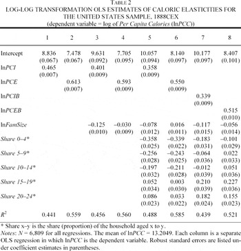
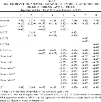
Tables 2 and 3 report OLS estimates of the income and expenditure elasticities of calories for the American and British samples, respectively. Odd numbered columns provide estimates of the income elasticity of calories and even numbered columns provide estimates of the expenditure elasticity of calories. The specifications in columns 1 and 2 in the tables are the simplest estimates of the elasticities. The log of family size is added to the model in columns 3 and 4, and its inclusion suggests that the true elasticities are lower once family size is controlled for.25
Note that the inclusion of the log of household size is appropriate only if household size has a level effect on the constant elasticity function; nonparametric results (not reported) confirm this.
The results of Tables 2 and 3 are robust to the inclusion of geographical and industry dummy variables (not reported).


For each specification (columns 1–8 in Tables 2 and 3), I reject the hypothesis that the British elasticities are less than or equal to the American elasticities at all conventional significance levels.27
Formal tests of the elasticity difference confirm these results. I pooled the data and regressed the log of per capita calories on the log of per capita income or expenditure and a term Γ(1(UK) * [lnPCI or lnPCE]) to test for a structural elasticity difference between the two samples. The hypothesis that Γ = 0 was rejected with t-statistics ranging from 4.78 to 8.61 for the regression models estimated in Tables 2 and 3. The exclusion of alcohol from total calories results in an understatement of the elasticities. For example, when alcohol is included as a source of calories the income elasticities reported in column 3 of Tables 2 and 3 become 0.6069 for the British sample and 0.4282 for the American sample.
Tables 2 and 3 show that the differences between the United States and Great Britain in the income elasticity of calories differences are greater than the differences in the expenditure elasticity of calories. It is straightforward to show why the differences in the income elasticity should be greater than the differences in the expenditure elasticity. First, note that the income elasticity, which we can call β, is equal to the income elasticity of expenditure (which we can call γ) multiplied by the expenditure elasticity of calories (which we can call θ). Mathematically, we can represent this with β = θ γ. Differences in the income elasticity are therefore Δ β = Δ (θ γ). If I assume that the income elasticity of expenditure (γ) is the same for both the United States and Great Britain, then it follows that Δ β = γ (Δ θ). If I further note that the income elasticity of expenditure (γ?) is empirically less than one but greater than zero, it follows that Δβ > Δ θ, implying that differences in the income elasticity of calories will be greater than differences in the expenditure elasticity of calories.
These differences in nutritional well-being are further supported by other aggregate measures of well-being. According to Marianne Ward and John Devereux real per capita GDP in the United States was 21 percent greater than British per capita GDP in 1891.29
Ward and Devereux, “Measuring British Decline.”
These estimates are based on per capita GDP estimates from Officer, “Annual Real and Nominal GDP”; and Johnston and Williamson, “Annual Real and Nominal GDP.”
Steckel, “Health.”
Steckel, “Stature and the Standard of Living.”
Further nutrition-based evidence bolsters the plausibility of the calorie demand elasticity differential. D. J. Oddy notes that Drummond argued that British malnutrition at the time was “more rife in England than it had been since the great dearths of medieval and Tudor times.”33
Oddy, “Food,” p. 275.
Haines and Steckel, “Childhood Mortality.”
What is most interesting about these elasticity differentials is that they strengthen the general argument that, in a cross section, significant calorie elasticity differentials imply significant nutritional differentials between subsamples. The narrative description of American and British working-class nutrition strengthens this interpretation. Peter Shergold found that British families were nutritionally worse off than American families.35
Shergold, Working-Class Life.
Ibid., p. 187.
Other investigators found similar patterns among industrial households in the late nineteenth century and early twentieth century when looking at detailed household budgets. Although both American and European laborers were malnourished, observers noted that European industrial workers were more malnourished than their American counterparts. For example, Frank Streightoff estimated that one-third of all industrial households in the United States at the time were malnourished and that only a small fraction (less than 10 percent) received an adequate amount of protein.37
Streightoff, Standard of Living.
Ibid., p. 101.
Lees, “Getting and Spending.” Indeed, it is difficult to place the British elasticities against any others because the sample for this survey was from a different geographic location than the other studies that have analyzed British nutrition.
Relaxing the Parametric Assumptions
OLS estimates are only part of the story, however. Although the constant elasticity function has much to commend it, many have argued that the assumption of a constant elasticity is rather restrictive. Earlier, I posited that the calorie income and expenditure elasticities should decrease as income and expenditure increase, and yet the constant elasticity function, by assumption, negates this possibility. Nonparametric techniques are available to relax the constant elasticity function assumptions to make them more consistent with economic theory. Locally linear regressions were used to nonparametrically estimate the relationship between calories and income.
The locally weighted regression assumes that the functional relationship between y (calories) and x (income or expenditure) is linear within small local neighborhoods of x.40
More precisely, the local regression proceeds as follows. For each Xj a weighted regression is run using only the n′ = (0.3)n observations that that are closest to Xj in absolute value. The design matrix used in the regression is X*, a subset of X that contains only the elements that are within n′. The weighting matrix, W, is a n′ x n′ diagonal matrix whose diagonal elements are Wi are such that

, and this is known as a tricube weight. Within that neighborhood (of Xj) a weighted regression of y on x is run, with the weights equal to zero for values of x far away from Xj, and approaching one for x values close to Xj, and hence the actual neighborhood is smaller than 30 percent. For each Xj
a ŷj is determined by

where the beta vector is

. The total number of local regressions used in this procedure is therefore equal to n.
The value of 30 percent is also known as the smoothing parameter. The choice of smoothing parameter is debatable, and many researchers prefer large values. The larger the smoothing parameter, the greater the smoothness of the total function, but this is at the expense of recovering a function that is locally smooth, as the higher values of the smoothing parameter ensure a globally smooth function. My choice of smoothing parameter is relatively small compared to other nonparametric work, and this value is preferred because the nonparametric method adopted is used to recover local estimates of the elasticity.
Formally, I took Gij = (xmax – xmin) / 100 for j = American, British; i = log of per capita income, log of per capita expenditure. The local slope between the points is then (with the data sorted from one to n with one being the lowest value of x)

where by construction xk – xl = Gij. This type of estimation is simply attempting to numerically recover the derivative of the local regression function, which in a log-log transformation is the slope of the regression function, the elasticity. To be clear, first the local linear regression of y (calories) on x (income or expenditure) is performed, and this yields estimates of y for each value of x. Using the function generated by the local linear regression, the local slope, the estimate of the elasticity, is estimated over an evenly spaced grid in y,x space.
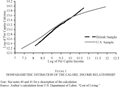
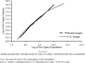
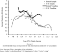
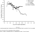
Figure 1 shows the locally weighted regression fitted values from the log of per capita calories on log of per capita income regression, and Figure 2 shows the fitted line for the local log of per capita calories on log of per capita expenditure regressions for both samples. As both Figures 1 and 2 show, the American and the British functions are nearly linear in both specifications, even with the relatively small neighborhoods in the local regressions, and this suggests that any potential information loss from the parameterization required by OLS will not be large. If we can take the slopes of these lines as rough estimates of the elasticities, we see that in Figure 1 the slope of the American line is close to 0.4, whereas for the British line it is close to 0.6, and in Figure 2 the slope is 0.6 for American households and 0.7 for British households. The steeper slopes of the British curves would imply that the British elasticities are greater than the American elasticities. Also note that the slope in Figures 1 and 2 are close to the elasticity estimates from the simple lnPCC on lnPCI, lnPCE regressions in columns 1 and 2 of Tables 2 and 3.

FIGURE 1 NONPARAMETRIC ESTIMATION OF THE CALORE, INCOME RELATIONSHIP

FIGURE 2 NONPARAMETRIC ESTIMATION OF THE CALORIE, EXPENDITURE RELATIONSHIP
Figure 3 shows the estimates of the local income elasticities of calories for the American and British samples. A six-degree polynomial trend line is included on the figure as well, and this trend line confirms that the elasticity does indeed decline with income. For the British households, the elasticity goes from a high of 0.7 at low incomes to a low of 0.55 at high incomes. For American households the elasticities go from a high of 0.6 to a low of 0.2. Figure 4 shows a similar trend for the expenditure elasticity of calories, although the expenditure elasticities are greater than the income elasticities. Both the American and British households have expenditure elasticities near 0.85 at low expenditures. The low point of expenditure elasticities of 0.65 for British households is seen at moderate expenditures, whereas the low point of expenditure elasticities for American households of near 0.35 is seen at high expenditures. Note that in both Figures 3 and 4 the elasticities are centered around the slopes of the lines in Figures 1 and 2, and these midpoints agree with the elasticity estimates in column 1 of both Tables 2 and 3. Overall, the nonparametrics show that these elasticities appear to behave as economic theory would predict.

FIGURE 3 NONPARAMETRIC ESTIMATES OF THE INCOME ELASTICITY OF CALORIES

FIGURE 4 NONPARAMETRIC ESTIMATES OF THE EXPENDITURE ELASTICITY OF CALORIES
EXPLAINING DIFFERENCES IN NUTRITIONAL WELL-BEING
What accounts for the large differential in calorie demand between the American and British? I take three approaches to this question. One method is demographic and descriptive, another is econometric, and the last considers relative prices. Demographically, I consider the household's income composition and the household head's occupation to see if the results hold across subgroups defined by their household income composition. Econometrically, I decompose the income elasticity of calories into two parts to meter out the contribution that income makes to the differences in calorie elasticities observed in Tables 2 and 3. Lastly, I compute the relative price of calories in both the United States and Great Britain.
Income Composition, Industry, and Calorie Elasticity Differentials
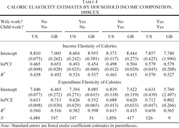
We should be mindful of the fact that the OLS results reported above are aggregate estimates of the elasticities and act as a summary measure of the population's elasticity. Table 4 presents results of the calorie elasticities estimated by household income composition.43
It must be noted that “wife working” includes only wives who earned income from an outside source. It does not include taking in a boarder or housework, which are surely a form of work.

Summary measures of income by type of income shed more light on the issue than the regression results reported in Table 4. Americans were wealthier than their British counterparts, but the difference narrows for the subgroups where wives and children work outside of the home. Although the overall United States-Great Britain per capita annual income differential is $34.55, for households where the husband is the only wage earner the difference grows to $50.79. This differential decreases to $9.56, however, when I compare the subsamples where children are working outside of the home and becomes negative (–$13.76) when wives work outside of the household. There is a substantial loss of income relative to British households when American wives and children work outside of the home. These facts, when viewed in conjunction with the results of Tables 2 and 3, imply that the elasticity differential is driven by the relatively high earnings of American men.
It would be unwise to argue that demographic composition accounts for the calorie elasticity differential when income composition between the two samples differs. British families were much more likely to send their children to work than American families. Whereas less than 30 percent of the American households had children who worked outside of the home more than 40 percent of British families had children in the labor market. Also, American fathers earned less than British fathers when their children worked outside of the home, although the total income ratio between countries for this group remains nearly equal to that for all families in the survey (120.41 percent versus 128.8 percent for all families). Also note that household size and age composition are included in the fullest specifications in Tables 2 and 3, and the elasticity differential remains.
Historical observers noted this trend as well. Streightoff and Robert Chapin held that American families with multiple wage earners were worse off than their single-earning counterparts among industrial households at the time.44
Streightoff, Standard of Living; and Chapin, Standard of Living.
Angus and Mirel, “From Spellers.” Schooling, in particular the spread of public education, was obviously an important institutional difference between the United States and Great Britain at the time. But insofar as public schools are funded by their local communities, they, too, reflect the underlying economic differences to a degree.
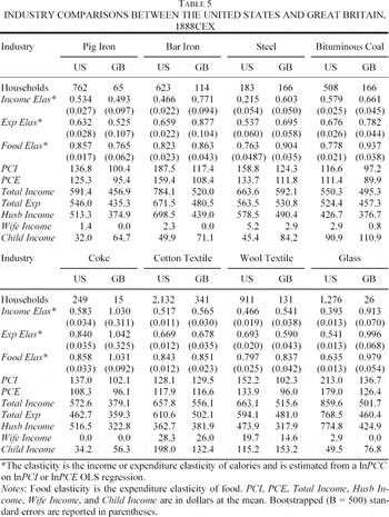
Table 5 displays the industry comparisons between American and British households.46
No families in the iron ore industry were surveyed in the British sample.

Due to small sample sizes for each industry, hypothesis tests are not very instructive as they have relatively little power; if I fail to reject the hypothesis of elasticity equality it could still be true that the elasticities are not close to one another. Nevertheless, I bootstrapped the sample variances of the income and expenditure elasticities of calories by industry, which were calculated with an OLS regression of the log of per capita calories on the log of per capita income and the log of per capita expenditure, respectively, so such a test could be performed with the best possible estimate of the standard errors. The rejection of the hypothesis that the British elasticities are less than or equal to the American elasticities is fairly robust to the within-industry comparison, which tells us that the results presented here are not due to the industrial composition of the data.
There were, however, large differences in the size of the calorie elasticity differential by industry. In some industries, such as glass and steel, the hypothesis was rejected at all conventional significance levels. For other industries, such as cotton textiles, the hypothesis is rejected only at the 10 percent significance level for the income elasticity, and not rejected for the expenditure elasticity. The general trend, however, was one of rejection of the hypothesis at least at the 10 percent significance level when the point estimate of the American elasticity was less than the British point estimate of the elasticity. Because the tests lack power, however, it is not clear how a failure to reject the hypothesis that the British elasticities are less than or equal to the American elasticities should be interpreted.
In addition to calorie elasticities, Table 5 also reports the expenditure elasticity of food. The differences in the food elasticity, for the most part, mirror those of the calorie elasticities, but they are usually much greater than the calorie elasticities. There are some important distinctions, however. In the Bar Iron industry, for example, the food elasticities are close to one another but the calorie elasticities are relatively far apart. This may be a situation where inference based upon the food elasticity will be different from the conclusions drawn from the calorie elasticity. As in the case of household income composition, the hypothesis that the American and British caloric elasticities are equal to one another is rejected when the per capita incomes of the British and American subgroups were highly dissimilar.
Decomposing the Income Elasticity of Calories
How much of the income elasticity of calories differential is due to differences in per capita income? To reach such a measure I decompose the income elasticity of calories, which can be used to estimate the share of the differential due to average income differences between the American and British households. Decomposition of the income elasticity of calories proceeds as follows. First, note that in the log-log transformation I assume that the expected log of per capita calories is a linear function of income

and further assume the expected log of per capita expenditure is a linear function of income

With the above in hand, it is easy to see how the expected log of per capita calories can be written as a function of expenditure, where

This function of expenditure is itself a function of income

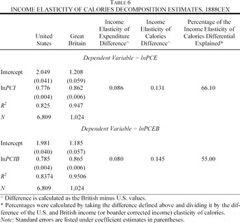
decomposing the income elasticity of calories, β, into two parts. The first term, θ, is the expenditure elasticity of calories. The second term, γ, is the income elasticity of expenditure. The contribution that the income differential makes to the income elasticity of calories differential is estimated by

If the United States and Great Britain lie on the same expenditure-income curve, such that differences in their income elasticities of expenditure are due entirely to average income differentials, the contribution of the income elasticity of expenditure differential to the income elasticity of calories differential is roughly the amount of the nutritional well-being difference that is explained by the income differentials between the United States and Great Britain.
47Nonparametric analysis revealed that the expenditure-income relationship is indeed linear, and that the American and British expenditure-income relationships appear to be part of the same linear function, but centered at different average income values.
Table 6 shows the results of the OLS regressions for the income elasticity of expenditure, and uses the differentials to compute the portion of the income elasticity of calories differentials explained by the difference of the income elasticities of expenditure. The income differentials explain more than 65 percent of the differential for the per capita income based elasticity estimates and 55 percent of boarder-corrected per capita income based estimates. The majority of the caloric elasticity differential is driven by differences in income between the two groups. The wage premium enjoyed by workers in the United States at the time has been shown, then, to have a large impact on the nutritional well-being of American families.

In some respects, this decomposition asserts that the differences in nutritional well-being are largely due to the fact that the American income distribution in the 1888CEX has a larger and wider right tail. Furthermore, the results of Table 6 confirm the validity of the decomposition. When one multiplies the income elasticity of expenditure estimate and the expenditure elasticity of calories estimates, the product is nearly the same as the income elasticity of calories estimates from OLS, which is found in column 1 of Tables 2 and 3.
The Relative Price of Calories
One explanation for the differences in nutritional well-being between the United States and Great Britain could be differing prices of calories. Because calories (food) have few substitutes, increases in income act as a decrease in the relative price of the item. If we can think of the market as being divided between food and nonfood items, and knowing that under Walras's Law demand elasticities must sum to one, a high relative price of calories (food) crowds out the demand for other items because food is necessary for survival. If it were true that calories were more costly in Great Britain than in the United States, and without good substitutes for food in the market, households in Great Britain will respond more strongly to income changes than those in the United States. We could think of households as substituting away from the relatively more expensive items (in this case, calories), but in the case of calories substituting away from food would cause families that are already malnourished to be even more so, and this would be implausible.48
This is not to say that there would be no substitution effect, but considering the malnourished state of the households considered here, the substitution effect would be small.
To measure the price of a calorie I construct a calorie price index. Construction of the calorie price index starts by noting that the calorie price faced by households must be weighted by the share that a particular food has in the total diet. Average calorie price should be estimated by household, as each household faces a different average calorie price depending on its diet. Therefore, the calorie price for each household k is constructed to be

where pic is the price of a calorie from food i and where

is the share of total calories belonging to food i. The average calorie price faced by all households in either the United States or Great Britain is therefore

. It is important to note that this construction of the calorie price causes the relative price of calories to be endogenous. Because we know that American households were wealthier than British households we could surmise that British households would purchase less expensive calories than American households. In this way, the relative prices reported below are lower bounds—relative prices constructed from a fixed basket would lead to larger relative price differences between the United States and Great Britain, because it would not reflect a poorer household's ability to substitute to cheaper calories.
To compare the price of calories to the prices of other goods one could construct a price index for all goods in the economy. Such an index, however, would include many items that were not consumed by industrial households in the late nineteenth century. Any inferences drawn from a comparison based on such an index, then, could be due to prices that have very little connection to household consumption. Taking a more microeconomic approach, I compare the calorie price to the prices of 29 standard household items. The prices of these household items come from the Aldrich report, and the goods are matched items, so that quality has been controlled for as much as possible.49
The “Rent of One Room” price comes from the 1888CEX. It is the rent expenditure of the household divided by the number of bedrooms in the household.
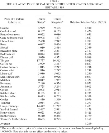
Table 7 shows the calorie price in both the United States and Great Britain relative to the price of the 29 common household items. It also computes the relative calorie price between the United States and Great Britain for the 29 household items. As the table shows, both the mean and median of the relative prices show that calories are 20 percent more expensive in Great Britain than they are in the United States. In terms of trends, it does appear that relative to household furniture (tables, chairs, bedroom sets, etc.) calories are cheaper in Great Britain, but when compared to most other items calories are cheaper in the United States.

The large difference in the relative price of calories is surprising when one considers the endogenous nature of this calorie price measure. As stated earlier, this calorie price differential understates the true difference in the relative cost of food between the United States and Great Britain in the late nineteenth century. This large difference in the cost of calories is obviously a large part of the story of the nutritional differences. Although the decomposition showed that income differences explained more than half of the elasticity differential, such large differences in the relative price of calories must certainly explain a large part of the remaining differential. Given their lower wages and relatively high cost of calories, it would certainly be reasonable to assert that British families should have higher demand for calories than American households.
The results discussed in this section establish a number of patterns. First, there were significant differences in aggregate measures of nutritional well-being between American and British households in the late nineteenth century. As the household income analysis has shown, this differential was largely driven by income differentials, usually the husband's. Proxies such as income, however, understate the differential in nutritional well-being. In decomposing the elasticity I found that income differentials explained more than half of the expenditure elasticity of calories differential, but left a great deal of the differential unexplained. Even with the same income, we would expect there to be a sizable gap in calorie demand between the United States and Great Britain. Lastly, we saw that calories were much more expensive in Great Britain than in the United States in the late nineteenth century. The relative price differential was quite large, and this gap in the relative price of calories probably explains a large part of the elasticity differential unexplained by income alone.
CONCLUSION
This article has shown that the microeconometric approach currently favored in development economics can successfully extend and deepen our understanding of nutritional well-being in the past. In particular, we now have new insight into nutritional well-being in the late nineteenth century and strong clues to why the calorie elasticity differential existed between the United States and Great Britain. Calorie elasticities have revealed that American nutrition in the late nineteenth century was much better than British nutrition at the time. The empirical findings presented here agree with the narrative evidence, and they also support the notion that caloric elasticities are indeed an advantageous way to quantify nutritional well-being.
In attempting to explain the calorie elasticity difference I found that income played a large and dominant role, but that relative prices were an important piece of the puzzle as well. In looking at the income composition of the household I found that the earnings of the household head, usually the male, were the primary source of the income differential. Industry analysis further revealed that the elasticity differential is most pronounced in industries where the wage gaps between British and American workers were pronounced. This is what we would expect both from economic intuition and from the narrative record.
One of the main findings in this work is that income only explains 60 percent of the caloric elasticity differential between the United States and Great Britain in the late nineteenth century. This finding tells us that more than income convergence was needed to close the nutritional gap between the United States and Great Britain. The remaining difference is probably due to the differences in the relative price of calories. We saw that the relative price of calories was more than 20 percent greater in Great Britain than in the United States. These relative price differentials tell us that the elasticity behaves the way that the relative prices predict. Food was much dearer to consumers in Great Britain both because it was more expensive and because they were poorer than their American counterparts.
I thank Raj Arunachalam, Andrea A. Cann, Dora L. Costa, William A. Darity Jr., J. Bradford DeLong, Ronald D. Lee, Thomas Logan Sr., Edward A. Miguel, Muna S. Meky, Martha L. Olney, James L. Powell, Christina D. Romer, Kenneth W. Wachter, two anonymous referees, and numerous seminar participants for extremely helpful discussions and comments on various aspects of this work. Dora L. Costa, Michael R. Haines, and Richard H. Steckel alerted me to data sources. Portions of this research were supported by the National Institute of Child Health and Human Development. All views expressed herein and errors, both of omission and commission, are my own.