1 Introduction
Lorenz presented in [Reference Lorenz30] an example of a parameterized 2-degree polynomial system of differential equations, as in equation (1), as a very simplified model for the convection of thermal fluid, motivated by an attempt to understand long-term weather forecasting. The concrete model can be stated as
 $$ \begin{align} (\dot{x}, \dot{y}, \dot{z})= (10(y-x), 28x-y-xz, xy-8/3z). \end{align} $$
Numerical simulations for an open neighborhood of the chosen parameters suggested that almost all points in the phase space tend to a strange attractor, nowadays called the Lorenz attractor. Ever since its discovery in 1963, the Lorenz attractor has been playing a central role in the research of singular flows, that is, flows generated by smooth vector fields with singularities, that is, points where the flow vanishes. However, Lorenz’s equations turned out to be very resistant to rigorous mathematical analysis, from both conceptual (existence of a singularity accumulated by regular orbits prevents the attractor from being hyperbolic) as well as numerical (solutions slow down as they pass near the singularity, which means unbounded return times and, thus, unbounded integration errors) points of view [Reference Sparrow54]. Moreover, for almost every pair of nearby initial conditions, the corresponding solutions move apart from each other exponentially fast as they converge to the attractor. That is, the attractor is sensitive to the initial conditions. This unpredictability is a characteristic of chaos. Most remarkably, this attractor is robust: it can not be destroyed by any small perturbation of the original flow.
A very fruitful approach was undertaken, independently, by Afraimovich, Bykov, and Shil’nikov [Reference Afraimovich, Bykov and Shil’nikov1, Reference Afraimovich, Bykov and Shil’nikov2], and by Guckenheimer and Williams [Reference Guckenheimer and Williams23, Reference Williams62]. They constructed a geometric Lorenz attractor that reproduces the behavior observed by Lorenz. As an abstract object, the geometric Lorenz attractor is the inverse limit of a semiflow on a branched
 $2$
-manifold (with boundary). The flow has a singularity, on the boundary of the surface, and orbits leaving a neighborhood of this singularity follow either of two branches which return to (and are glued together along) an interval of branch points transverse to the stable manifold of the singularity. From the geometrical point of view, geometric Lorenz attractors are flows on the three-dimensional space that contain a singularity accumulated by regular orbits, that is, orbits
 $\gamma $
where
 $X^t(x)\neq 0$
for all
 $x\in \gamma $
and
 $t>0$
. They have a natural cross-section given by a two-dimensional square crossed by all orbits of the flow inside the attractor except the singularity.
While the discovery of the Lorenz attractor leveraged fundamental developments in Dynamical Systems, the equations in equation (1) themselves have continued to resist all the attempts to prove that they exhibit a sensitive attractor. Bunimovich and Sinai [Reference Bumimovich, Sinai and Gaponov-Grekhov13, Reference Sinai51] have indicated a program that could prove that the Lorenz equations have a transitive attractor.
Rychlik and Robinson gave a proof for the so-called Shilnikov criteria [Reference Shilnikov50] providing necessary and sufficient conditions for the birth of the Lorenz attractor from certain classes of codimension-3 bifurcation (codimension-2 bifurcations for systems with the Lorenz symmetry) [Reference Robinson46, Reference Robinson47, Reference Rychlik49]. From the bifurcation point of view, in addition to these results, we cite the works in [Reference Gonchenko, Shilnikov and Turaev20, Reference Kazakov28, Reference Li and Turaev29, Reference Lyubimov and Zaks32, Reference Morales, Pacifico and San Martin38, Reference Morales, Pacifico and San Martin39, Reference Robinson48].
A successful approach for the Lorenz flow was through rigorous numerics. Many authors have performed numerical simulations of these equations, and the book by Sparrow gives an account of many of these results proved in the 1970s [Reference Sparrow54]. Later, in this way, it was proved [Reference Hassard, Hastings, Troy and Zhang25, Reference Hastings and Troy26, Reference Mischaikow and Mrozek34, Reference Mischaikow and Mrozek35] that the Lorenz system of equations exhibits a suspended Smale horseshoe [Reference Smale52]. It implies, in particular, the existence of infinitely many closed orbits. However, proving the existence of an attractor as in the geometric models is an even harder task. Indeed, one cannot avoid the fact that solutions slow down as they pass near the singularity, which, as said before, means unbounded return times and unbounded integration errors, see [Reference Sparrow54, Reference Tucker57]. This was finally settled by Tucker in [Reference Tucker56, Reference Tucker57] around the turn of the century.
The theory of dynamical systems indicates that the way to analyze the equations in equation (1) is to prove that they possess a strong stable foliation. For the geometric model of the Lorenz equations proposed by Guckenheimer and Williams in [Reference Guckenheimer and Williams23, Reference Williams62], an invariant
 $C^1$
strong stable bundle and the resulting strong stable foliation are assumed to exist. With this assumption, the theory of normally hyperbolic attractors allows one to show that an attractor exists. It also gives a criterion to check if it is transitive. Once the strong stable foliation is known to exist with the right set of expansion rates for one set of equations, then they persist for perturbations of the equations; see [Reference Guckenheimer and Williams23, Reference Robinson45, Reference Williams60, Reference Williams61] for a discussion of the geometric equations and the resulting attractor. Recently, in [Reference Smania and Vidarte53], the authors proved the existence of
 $C^k$
-invariant foliations for Lorenz-type maps. Nowadays, in the literature, there is an expressive number of results about the Lorenz geometric attractor, both from the geometric as well as the measure-theoretic points of view, and we refer the reader to see [Reference Araújo and Pacifico9, Reference Araújo, Pacifico, Peixoto, Pinto and Rand10, Reference Guckenheimer, Marsden and McCracken21, Reference Guckenheimer and Holmes22, Reference Ovsyannikov and Turaev41, Reference Viana58] and references therein.
In the 1990s, a breakthrough was obtained by Morales, Pacifico, and Pujals [Reference Morales, Pacifico and Pujals37], following the very original ideas developed by Mañé in the proof of the
 $C^1$
stability conjecture [Reference Mañé33]. They provide a characterization of robustly transitive attractors for three-dimensional flows, of which the Lorenz attractor is the more significant example.
After this seminal work, significant advances in this theory were achieved through the work of many authors, who gradually turned to the statistical and stochastic points of view of the Lorenz attractor, see [Reference Araújo4–Reference Araújo and Melbourne6, Reference Araújo, Melbourne and Varandas8, Reference Araújo, Pacifico, Peixoto, Pinto and Rand10–Reference Araújo and Varandas12, Reference Galatolo, Nisoli and Pacifico17, Reference Galatolo and Pacifico18, Reference Luzzatto, Melbourne and Paccaut31, Reference Pacifico and Todd43, Reference Pacifico, Yang and Yang44].
Taking into account that the divergence of the vector field induced by the system in equation (1) is negative, it follows that the Lebesgue measure of the Lorenz attractor is zero. Henceforth, it is natural to ask about its Hausdorff dimension. Numerical experiments give that this value is approximately equal to 2.062 (cf. [Reference Viswanath59]) and also, for some parameters, the dimension of the physical invariant measure lies in the interval
 $[1.24063,1.24129]$
(cf. [Reference Galatolo and Nisoli16]). In [Reference Afraimovich and Pesin3, Reference Steingenber55], this dimension is characterized in terms of the pressure of the system and in terms of the Lyapunov exponents and the entropy concerning a good invariant measure associated with the geometric model. However, in both cases, the authors prove that the Hausdorff dimension is greater or equal than
 $2$
, but not necessarily strictly greater than
 $2$
. A first attempt to obtain the strict inequality was given in [Reference Mora and Lizana36], where the authors achieve this result in the particular case that both branches of the unstable manifold of the singularity meet the stable manifold of the singularity. Finally, in [Reference Moreira, Pacifico and Romaña Ibarra40], the authors prove that the Hausdorff dimension of a geometric attractor is strictly greater than
 $2$
.
Despite all this progress, we still are far from a topological classification of singular hyperbolic attracting sets in dimension
 $3$
. Moreover, there is also a huge gap in the understanding of unfolding parameterized families of singular hyperbolic attractors in any dimension.
The Lorenz attractor has a unique hyperbolic singularity, whose strong stable manifold
 $W^{ ss}(\sigma )$
separates the stable manifold
 $W^{s}(\sigma ) $
into components, called the upper and lower local stable sets of
 $\sigma $
. One of these local stable sets is disjoint from the attractor. These properties are shared by the geometrical Lorenz model.
This paper was motivated by a question from Adriana da Luz to the second author. How can one construct a three-dimensional flow presenting a singular hyperbolic attractor, containing a unique Lorenz-like singularity
 $\sigma $
, intersecting robustly upper and lower local stable sets of
 $W^{s}(\sigma ) \setminus W^{ss}(\sigma )$
? One can easily construct examples exhibiting this phenomenon. Among those, a particular one displays a very intriguing behavior under perturbations. The goal of the present paper is to address this matter. That is, this work aims to build an open set of vector fields for which the attractors have intersections with the upper, lower, and both local stable sets.
We describe a
 $C^1$
-open set
 ${\mathcal O}_1$
of vector fields on a three-dimensional space having a common attracting region U which contains a unique singularity
 $\sigma $
of Lorenz type, see Definition 2.3. As in the geometric Lorenz attractor, each flow
 $X \in {\mathcal O}_1$
has a global cross-section
 $\Sigma $
, which is a topological annulus, and a first return map
 $P:\Sigma \to \Sigma $
possessing an invariant stable foliation
 $\mathcal {F}^s$
. The intersection of the stable manifold of
 $\sigma $
with the cross-section splits
 $\Sigma $
into two connected components,
 $\Sigma ^1$
and
 $\Sigma ^2,$
and the intersection of the upper (lower) stable component of
 $W^{s}(\sigma )$
contains each a segment,
 $\gamma ^s_+$
and
 $\gamma ^s_-$
, respectively, transverse to the boundary
 $\partial \Sigma $
and connecting the two boundary components of the annulus
 $\Sigma $
. We denote the upper (lower) stable component of
 $W^{s}(\sigma )\setminus W^{ss}(\sigma )$
by
 $W^s_+(\sigma )$
(
 $W^s_-(\sigma )$
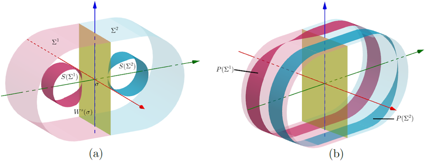
), respectively, see Figure 1. We assume that both
 $\gamma ^s_+$
and
 $\gamma ^s_-$
belong to
 $\mathcal {F}^s$
. The unstable manifold of
 $\sigma $
is one-dimensional and
 $W^u(\sigma )\setminus \{\sigma \}$
consists of two separatrices
 $W^u_i(\sigma ), \, 1 \leq i \leq 2,$
each one having a first intersection point
 $q_i$
with
 $\Sigma $
. See Figure 1.
The diagram displays
 $\Sigma = \Sigma ^1 \cup \Sigma ^2$
and
 $W^s(\sigma ) \setminus W^{ss}(\sigma )=W^s_{+}(\sigma ) \cup W^s_{-}(\sigma )$
, and the points
 ${q_i, 1\leq i \leq 2,}$
defined above.

The first result gives the topological nature of the class of flows in
 $\mathcal {O}_1$
, whose attractor intersects just one or both components of the stable sets of
 $\sigma $
, proving the existence of three disjoint open and non-empty sets in
 $\mathcal {O}_1$
, roughly described as:
 $ \mathcal {L}^-$
, whose attractors intersect just
 $W^s_-(\sigma )$
;
 $\mathcal {L}^+$
, whose attractors intersect just
 $W^{s}_-(\sigma ) $
; and
 $\mathcal {L}^{-,+}$
, whose attractors intersect both
 $W^s_+(\sigma )$
and
 $W^s_-(\sigma )$
. We call the attractors in
 $\mathcal {L}^-$
down-Lorenz, the attractors in
 $\mathcal {L}^+$
as upper-Lorenz, and the attractors in
 $\mathcal {L}^{-,+}$
as two-sided Lorenz. We denote
 $\mathcal {L}^{-,+} \cup \mathcal {L}^+ \cup \mathcal {L^-}=\mathcal {L}$
. See §4.4 for the precise definitions of these sets.
Now, let us explain what we mean by a fake horseshoe. It consists of a sequence of operations on the unit square, quite similar to the horseshoe, the only difference being the way back to the square of the resulting folded rectangle: the bottom of the folded rectangle fits back like the top of the starting square. Figure 2 displays the main features of a fake horseshoe. Note that a fake horseshoe preserves the orientation, while the horseshoe does not.
The usual horseshoe and a fake horseshoe.

Theorem A. Any vector field
 $X\in {\mathcal L}^+$
admits exactly two chain recurrence classes: one is an upper-Lorenz attractor and the other is a hyperbolic basic set, topologically equivalent to the suspension of a fake horseshoe. The symmetric statement holds for
 ${\mathcal L}^-$
, interchanging the upper for the down.
A saddle p (that is, a hyperbolic singularity point with non-trivial stable and unstable bundles) of a flow has a homoclinic tangency if its stable and unstable manifolds have some non-transverse intersection. In this case, we say that p has a homoclinic loop. Two saddles with different u-indices (that is, dimension of the unstable bundle) have a heterodimensional cycle if their stable and unstable manifolds intersect cyclically (by dimension deficiency, one of these intersections is necessarily non-transverse), see [Reference Díaz15].
Two saddles of a
 $C^1$
vector field
 $ X $
are homoclinically related if the invariant manifolds of their orbits intersect transversely and cyclically. To be homoclinic related defines an equivalence relation on the set of saddles of X. Two saddles that are homoclinically related have the same u-index. The homoclinic class of a saddle p of X is the closure of the saddles of X that are homoclinically related to p. A homoclinic class is a transitive set (that is, it contains a point whose orbit is dense in the set).
Consider
 ${\mathcal H}^i\subset {\mathcal O}_1$
,
 $i=1, 2$
, the hypersurface corresponding to the vector fields X for which the first intersection point
 $q_i$
of
 $W^u_i(\sigma )$
with
 $\Sigma $
belongs to
 $\gamma ^s_+\cup \gamma ^s_-$
. In other words, X belongs to
 ${\mathcal H}^i$
if
 $\sigma $
admits a homoclinic loop for the unstable separatrices
 $W^u_i(\sigma )$
so that the homoclinic loop cuts
 $\Sigma $
at a unique point
 $q_i$
(see Figure 1).
Theorem B. For any
 $X\in {\mathcal O}_1$
in one of the hypersurfaces
 ${\mathcal H}^1$
or
 ${\mathcal H}^2$
, the maximal invariant in U is a transitive singular attractor meeting both stable sets
 $W^s_{-}(\sigma )$
and
 $W^s_{+}(\sigma )$
.
The statement of the theorem above does not announce a two-sided Lorenz attractor, because the hypersurface
 ${\mathcal H}^i, i= 1, 2,$
is not an open subset, and then the robustness of the transitivity is not ensured. We split each
 ${\mathcal H}^i$
into two
 ${\mathcal H}^i={\mathcal H}^i_+\cup {\mathcal H}^i_-$
according to
 ${\{q_i\in \gamma ^s_+\}}$
and
 $\{q_i\in \gamma ^s_-\}$
, respectively. We then prove the following result, which characterizes the topological nature of the attractors for flows in the hypersurfaces
 ${\mathcal H}^i_+$
and
 $ {\mathcal H}^i_-$
. There is still the case of a double homoclinic loop that occurs when both intersection points
 $q_1$
and
 $q_2$
of the unstable manifold of
 $\sigma $
with the cross-section fall in the same segment of the intersection of the upper (lower) stable component of
 $W^{s}(\sigma )$
with the cross-section.
We denote by
 ${\mathcal H}^{1,2}_+$
the collection of flows in
 $\mathcal {O}_1$
such that
 $q_1,q_2\in \gamma ^s_+$
. Similarly, we denote by
 ${\mathcal H}^{1,2}_-$
the collection of flows in
 $\mathcal {O}_1$
such that
 $q_1,q_2\in \gamma ^s_-$
, see Figure 22 later. Thus, both unstable separatrices of
 $\sigma $
are homoclinic connections and are included in the same connected component of
 $W^{s}(\sigma ) \setminus W^{ss}(\sigma )$
. Clearly,
 ${\mathcal H}^{1,2}_+$
and
 ${\mathcal H}^{1,2}_-$
are codimension
 $2$
submanifolds included in
 ${\mathcal H}^1\cup {\mathcal H}^2$
. The next result ensures that for
 $X\in {\mathcal H}^i$
out of
 ${\mathcal H}^{1,2}_+$
and
 ${\mathcal H}^{1,2}_-$
, the transitivity of the attractor is robust, showing that the attractor is a two-sided Lorenz attractor.
Theorem C. If
 $X\in {\mathcal H}^i\setminus ({\mathcal H}^{1,2}_+ \cup {\mathcal H}^{1,2}_-)$
, there is a neighborhood
 ${\mathcal U}(X)$
of X such that the maximal invariant set for every
 $Y\in {\mathcal U}(X)$
is a two-sided Lorenz attractor.
Before we announce the next result, recall that
 $W^s_+(\sigma )$
(
 $W^s_-(\sigma )$
) is the upper (lower) stable component of
 $W^{s}(\sigma )\setminus W^{ss}(\sigma )$
and the sets
 $\mathcal {L}^+, \mathcal {L}^-, \mathcal {L}^{+,-}, \mathcal {L}$
are as above.
Theorem D. For any
 $X\in {\mathcal L}^{+,-}$
, the maximal invariant set in
 $U(X)$
is a transitive singular hyperbolic attractor meeting
 $W^{s}_{-}(\sigma )$
and
 $W^s_{+}(\sigma )$
. That is, it is a two-sided Lorenz attractor.
From our construction, we get that every
 $X \in \mathcal {L}$
contains a robust attractor (that is, there exists an open neighborhood
 $\mathcal {U}$
of X in the space of vector fields such that every
 $Y \in \mathcal {U}$
has an attractor). In addition to that, although the complement of
 $\mathcal {L}$
in
 $\mathcal {O}_1$
is non-empty, it has an empty interior. Thus, the next step is to understand the reasons why an attractor stops intercepting just one component of
 $W^{s}(\sigma )\setminus W^{ss}(\sigma )$
and suddenly starts to intersect both (and vice versa).
We will see that this phenomenon occurs due to the appearance of certain types of homoclinic and heteroclinic connections related to the position of the intersection points
 $q_1,\,q_2$
of
 $W^u_i(\sigma )$
with the cross-section.
Recall that
 $\Sigma $
is split into two connected components
 $\Sigma ^1$
and
 $\Sigma ^2$
, determined by the intersections of
 $W^{s}(\sigma )$
with
 $\Sigma $
. Assuming that the first return map has an expansion rate greater than the golden number
 $\varphi =({1+\sqrt {5}})/{2}$
, when
 $q_i$
falls into
 $\Sigma ^j$
with
 $i \neq j$
, the Poincaré map has a fixed point
 $p_i\in \Sigma ^j$
. Typically, a heteroclinic cycle arises when
 $q_i$
belongs to the stable leaf
 $W^s_j$
through
 $p_j$
.
We denote by
 ${\mathcal O}_{\varphi }$
the subset of flows in
 ${\mathcal O}_{1}$
for which the first return map has an expansion bigger than
 $\varphi $
, note that
 $\Sigma \setminus (W^s_1 \cup W^s_2)$
splits into two connected components
 $\Sigma _{-}$
and
 $\Sigma _{+}$
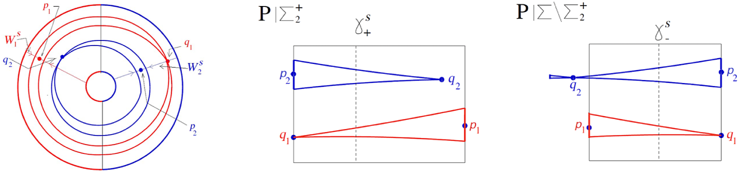
, see Figure 3. Let
 ${\mathcal H}{\mathcal E}_i \subset {\mathcal O}_{\varphi }$
be the subset of flows corresponding to the vector fields X for which
 $q_i\in W^s_j$
. In other words, for
 $X\in {\mathcal H}{\mathcal E}_i$
, the unstable separatrix of
 $\sigma $
corresponding to
 $q_i$
is a heteroclinic connection with
 $p_j$
. The subsets
 ${\mathcal H}{\mathcal E}_i$
are codimension
 $1$
submanifolds of
 ${\mathcal O}_\varphi $
.
 $ \Sigma _+$
and
 $\Sigma _-$
: determined by
 $W_1$
and
 $W_2$
, the stable manifolds of
 $p_1$
and
 $p_2$
, respectively.

Theorem E. For any
 $X\in {\mathcal H}{\mathcal E}_1\cap {\mathcal H}{\mathcal E}_2$
, there is a unique chain recurrence class, which is not transitive. Both
 $\Sigma _-$
and
 $\Sigma _+$
are invariant by P. The maximal invariant set of the restriction of P to
 $\Sigma ^i, 1\leq i \leq 2,$
is transitive: every unstable segment in
 $\Sigma ^i$
has its iterates which cut every segment in
 $\Sigma ^i$
. The open set U splits into two regions, each containing a full Lorenz (see Definition 2.9), intersecting along
 $W^s(p_1)\cup W^s(p_2)\cup W^u(\sigma )$
. See Figure 20 later.
A similar construction for a full Lorenz was observed in [Reference Gonchenko, Karatetskaia, Kazakov and Kruglov19] where it was called conjoined Lorenz twins.
The goal now is to describe the drastic changes in the behavior appearing in the topological dynamics when a family
 $X_\mu , \, \mu =(\mu _1,\mu _2) \in [-1,1]^2, $
crosses the boundary of the regions considered in Theorems A, B, C, D, and E.
We can refine the analysis of the topological behavior of flows in
 ${\mathcal O}_{\varphi }$
based on the position of
 $q_{1}$
and
 $q_{2}$
in
 $\Sigma $
. This introduces a new region, denoted by
 $\widetilde {{\mathcal O}_\varphi }^{+,+}$
, defined as the open subset where
 $q_1$
and
 $q_2$
belong to different components
 $\Sigma _\pm $
and
 $\Sigma _\mp $
.
The behavior of the topological dynamics in all these regions is established in the next theorem.
Theorem F. With the previous notation, we obtain the following:
-
• the vector field
 $X_\mu $
belongs to
${\mathcal L}^+$
if and only if
$\mu $
belongs to the quadrant
${\mu _1>0, \mu _2>0}$
. In other words, the upper full Lorenz of
$X_{0,0}$
becomes a (robust) Lorenz attractor, and the down full Lorenz of
$X_{0,0}$
becomes a fake horseshoe;
-
• the vector field
$X_\mu $
belongs to
${\mathcal L}^-$
if and only if
$\mu $
belongs to the quadrant
${\mu _1<0, \mu _2<0}$
. In other words, the upper full Lorenz of
$X_{0,0}$
becomes a (robust) Lorenz attractor, and the down full Lorenz of
$X_{0,0}$
becomes a fake horseshoe; -
• the vector field
$X_\mu $
belongs to
$\widetilde {{\mathcal O}_\varphi }^{+,+}$
if and only if
$\mu $
belongs to the quadrant
${\mu _1<0, \mu _2> 0}$
or the quadrant
$\mu _1>0, \mu _2<0$
. In other words, the two full Lorenz of
$X_{0,0}$
merges into a two-sided Lorenz attractor.


The next theorem in the paper reads as follows.
Theorem G. With the previous notation, considering a
 $1$
-parameter family
 $ X_{\mu =(\mu _1,\alpha \mu _1)}$
for some
 $\alpha>0$
, we obtain the following:
-
• for
$\mu _1<0$
, the vector field admits a down Lorenz attractor and an upper fake horseshoe; -
• when
$\mu _1=0$
, the fake horseshoe becomes a full Lorenz and, simultaneously, enters in collision with the upper Lorenz attractor, which becomes a full Lorenz; -
• for
$\mu _1>0$
, the upper full Lorenz becomes a fake horseshoe when the down full Lorenz becomes a robust Lorenz attractor.


Figure 4 describes the main features established in Theorems F and G.
The bifurcation diagram of flows in
 $\mathcal {O}_{\varphi }$
.

Next, we study in greater depth the topological nature of a flow in
 $\mathcal {O}_{1}$
. Recall that if
 $X\in {\mathcal O}_1$
, then it contains a unique singularity
 $\sigma $
of Lorenz type, see Definition 2.3. Moreover,
 $X $
has a global cross-section
 $\Sigma $
, which is a topological annulus and a first return map
 $P:\Sigma \to \Sigma $
possessing an invariant stable foliation
 $\mathcal {F}^s$
. The leaves of the foliation
 ${\mathcal F}^s$
are segments crossing
 $\Sigma $
(connecting the two boundary components of
 $\Sigma $
). The leaves space
 $\Sigma /{\mathcal F}^s$
is a (topological) circle
 ${\mathbb S}^1_X$
. The segments
 $\gamma ^s_+$
and
 $\gamma ^s_-$
are leaves of
 ${\mathcal F}^s$
and induce each a point
 $c_+$
and
 $c_-$
respectively, on
 ${\mathbb S}^1_X$
. We assume that X preserves
 ${\mathcal F}^s$
and thus the first return map P preserves the foliation
 ${\mathcal F}^s$
. As a consequence, P passes to the quotient as a map
 $f=f_X$
defined from
 ${\mathbb S}^1_X\setminus \{c_+,c_-\}$
to
 ${\mathbb S}^1_X$
. As in the geometric model, we will see that
 $f_X$
restricted to each interval of
 ${\mathbb S}^1_X\setminus \{c_+,c_-\}$
is a diffeomorphism.
As for the geometric model of the Lorenz attractor presented in [Reference Guckenheimer and Williams23], we will see that to any vector field in
 ${\mathcal O}_1$
, we can associate combinatorial data, called the itinerary of the discontinuities. These itineraries induce a semi-conjugacy of
 $(\Sigma , P)$
with
 $({\mathbb X},\mathfrak {S})$
, where
 $\mathfrak {S}$
is the shift map on
 ${\mathbb X}$
and
 ${\mathbb X}$
is an appropriate alphabet chosen to represent the crossing points of the unstable manifold of the singularity with the cross-section.
Being precise, P is defined on
 $\Sigma \setminus (\gamma ^s_+\cup \gamma ^s_-)$
which is not invariant under P. Thus we get conjugacy in the restriction of
 $\Sigma \setminus W^s(\sigma )$
. However, since the Poincaré map preserves a stable foliation and the itineraries for the Poincaré map are functions of the stable leaf, they pass to the quotient on the leaves’ space, inducing itineraries for the one-dimensional quotient map. We use this symbolic analysis to show that each neighborhood of a flow in
 $\mathcal {O}_{1}$
, in the
 $C^{1}$
topology, contains flows whose attractor exhibits all of an uncountable family of topological types. As in the case of the geometric Lorenz attractor, we prove that this phenomenon is co-dimension two stable. The topological types exhibited by the various versions of this example can be distinguished by two parameters. Moreover, we construct a two-parameter family of flows in
 $\mathcal {O}_{1}$
which is
 $C^{1}$
stable. This is the content of our last result below.
Theorem H. The restrictions to the maximal invariant sets of X and
 $ Y \in \mathcal {O}_\varphi $
are topologically equivalent by a homeomorphism close to identity if and only if X and Y have the same itineraries.
This paper is organized as follows. Section 2 gives the concepts, definitions, and results proved elsewhere that will be needed in the text. Section 3, constructs the open set of flows
 ${\mathcal O}_{1}$
that will be analyzed in the remainder of the text. Section 4 gives the background and auxiliary results to prove the main results. In §5, we prove Theorems A, D, B, C, and E. In §6, we prove Theorems F and G. In §9, we prove Theorem H.
2 Preliminaries
2.1 Basic topological notions
Let
 $\mathfrak {X}^r(\mathbb {R}^3)$
,
 $\,r\geq 1,$
be the space of vector fields defined on
 $\mathbb {R}^3$
, with the
 $C^r$
topology. For
 $X \in \mathfrak {X}^r(\mathbb {R}^3) $
, we denote by
 $X^t$
the flow of X. If
 $U\subset M$
,
 $\overline {U}$
denotes the closure of U,
 $\operatorname {int} U$
the interior of U, and
 $\partial U$
the border of U. An invariant compact set
 $\Lambda $
of X is transitive if there is
 $p\in \Lambda $
so that its positive orbit is dense in
 $\Lambda $
(this notion is called topological ergodicity by some authors).
Recall that a sequence
 $\{p_i\}$
is an
 $\varepsilon $
-pseudo-orbit for X if there is
 $t_i>1$
such that
 $d(p_{i+1},X^{t_i}(p_i))<\varepsilon $
for all i. A point p is chain recurrent if for each
 $\varepsilon>0$
, there is a
 $\varepsilon $
-pseudo orbit
 $p=p_0,p_1,\ldots ,p_n=p$
. The recurrent chain set
 ${\mathcal R}(X)$
is the set of all chain recurrent points. It is a compact invariant set. An invariant compact set
 $\Lambda $
is chain recurrent or chain transitive if for every
 $\varepsilon>0$
, it admits an
 $\varepsilon $
-pseudo orbit
 $\{x_i\}$
,
 $x_i\in \Lambda $
, dense in
 $\Lambda $
.
Two points
 $p,q$
are chain equivalent if for any
 $\varepsilon>0$
, there are
 $\varepsilon $
-pseudo orbits from p to q and from q to p. Conley’s theory [Reference Conley, Cesari, Hale and Lasalle14] proves that chain-equivalence is an equivalence relation whose equivalence classes are called the chain recurrence classes. They define a partition of
 ${\mathcal R}(X)$
by invariant pairwise disjoint compact sets. A compact region U is attracting for a vector field X of
 $\mathbb {R}^3$
if its boundary is a codimension
 $1$
submanifold transverse to X and X is entering in U.
Definition 2.1
-
• A compact invariant set
$\Lambda _X$
of
$X^t$
is attracting if there exists an open neighborhood
$U \supset \Lambda _X$
which is an attracting region and such that
$\Lambda _X$
is the maximal invariant set in U, that is,
$$ \begin{align*}\Lambda_X= \underset{t>0}{\bigcap}X^t(U).\end{align*} $$
-
•
$\Lambda _X$
is an attractor if it is attracting and chain transitive (in particular,
$\Lambda _X$
is a chain recurrence class). -
•
$\Lambda _X$
is
$C^r$
robust if there is an attracting region
$U\supset \Lambda _X$
such that
$\Lambda _Y$
is an attractor of Y for every vector field Y which is
$C^r$
close to X. -
• An invariant compact set K is a quasi-attractor if it is a chain recurrence class and admits a basis of neighborhoods that are attracting regions. There is a decreasing sequence
$U_i\subset U_{i-1}$
of attracting regions so that
$K=\bigcap _i U_i$
.


Notice that the existence of an attractor is not ensured a priori. However, Conley [Reference Conley, Cesari, Hale and Lasalle14] proves the existence of quasi-attractors in any attracting region (for a vector field on a compact manifold).
Definition 2.2. Two vector fields X and Y defined on
 $\mathbb {R}^3$
are topologically equivalent if there exists a homeomorphism
 $h:\mathbb {R}^3 \to \mathbb {R}^3$
such that
 $h(\mathcal {O}_X(p))=\mathcal {O}_Y(h(p))$
and
 $\text {for all } p \in M$
and
 $\varepsilon>0, \text { there exists } \delta >0$
so that for
 $t \in (0,\delta )$
, there is
 $s \in (0, \varepsilon )$
satisfying
 $h(X^t(p))=Y^s(h(p))$
.
2.2 Singular points
A point p is singular if X vanishes at p, otherwise p is regular. The set of singular points of X is denoted by
 $\mathrm {Zero}(X)$
. A point
 $\sigma \in \mathrm {Zero}(X)$
is hyperbolic if the real part of the eigenvalues of
 $DX(\sigma )$
does not vanish.
Definition 2.3. A singularity
 $\sigma $
of X is Lorenz-like if the eigenvalues
 $\unicode{x3bb} _i \in \mathbb {R}, i \in \{ss, s, u\},$
of
 $DX(\sigma )$
satisfy
 $0<-\unicode{x3bb} _s<\unicode{x3bb} _{u}<-\unicode{x3bb} _{ss}$
.
Definition 2.4. In addition,
 $\sigma $
is non-resonant if for all
 $N>2$
and any choice of non-negative integer numbers
 $m_1,m_2,m_3$
with
 $2\le \sum _{j=1}^{3} m_j < N$
, we have
 $\sum _{j=1}^{3} m_j \unicode{x3bb} _j \neq \unicode{x3bb} _i$
.
Hartman Grobman’s theorem asserts that a vector field is locally topologically equivalent to its linear part in a small neighborhood of a hyperbolic singular point [Reference Hartman24]. Then Sternberg provides conditions to guarantee that this local topological equivalence is true of class
 $C^2$
.
Theorem 2.5. Let X a vector field and let
 $n \in \mathbb {Z}^+$
be given. Then there exists an integer
 $N = N(n) \ge 2$
such that if A is a real non-singular
 $d \times d$
matrix with eigenvalues
 $\unicode{x3bb} _1, \ldots ,\unicode{x3bb} _d$
satisfying

for any choice of non-negative integers
 $m_1,m_2 \ldots m_d$
, and if the application
 ${X(v)=A(v)+\psi (v)}$
and
 $\psi $
is of class
 $C^n$
for small
 $\|v\|$
with
 $\psi (0)=0$
and
 $\partial _v\psi (0)=0$
, then there exists a
 $C^N$
diffeomorphism from a neighborhood of
 $v = 0$
to a neighborhood of
 $\xi = 0$
that define a topologic conjugation between X and A.
Furthermore, the linearizing diffeomorphisms depend continuously on the
 $C^2$
topology from the vector field X, see for instance [Reference Pacifico42, Corollary in the Appendix] which provides a stronger statement.
2.3 The shift map
$\mathfrak {S}$

We consider
 ${\mathbb X}=\{A_0,A_1,B_0,B_1\}^{\mathbb N}$
the space of infinite positive words in the alphabet
 $\{A_0,A_1,B_0,B_1\}$
. We endow the alphabet
 $\{A_0,A_1,B_0,B_1\}$
with the total order
 $A_0<A_1<B_0<B_1<1.$
We endow
 ${\mathbb X}$
with the corresponding lexicographic order that we denote by
 $\prec $
(and
 $\preccurlyeq $
for the non-strict order). The shift map
 $\mathfrak {S} : {\mathbb X} \to {\mathbb X}$
is defined as
 $$ \begin{align*} (w_j)_{j\geq 0} \in {\mathbb X} \mapsto \mathfrak{S} (w_j)_{j\geq 0}= (w_{j+1})_{j\geq 0}.\end{align*} $$
We also define the star map (denoted by
 $\star $
) on
 ${\mathbb X}$
as follows: given a sequence
 ${w \kern1.3pt{=}\kern1.3pt(w_0, w_1,\ldots )\in {\mathbb X}}$
and a letter
 $L \kern1.3pt{\in}\kern1.3pt \{A_0,A_1,B_0,B_1\}$
, we set
 $ L \star w \stackrel {\scriptscriptstyle \mathrm {def}}{=} (L, w_0, w_1, \ldots ). $
2.4 Hyperbolic notions
Definition 2.6. Let X be a vector field of a manifold M. A compact invariant set
 ${\Lambda \subset M\setminus \mathrm {Zero}(X)}$
is hyperbolic if the tangent bundle
 $TM|_\Lambda $
over
 $\Lambda $
admits a splitting
 $TM|\Lambda = E^s\oplus {\mathbb R} X\oplus E^u \ \mbox {such that:}$
-
• the bundles
$E^s$
and
$E^u$
are continuous and invariant under the derivative of the flow; -
• there exists
$ T>0$
so that
$\text {for all } p\in \Lambda $
and
$\text {for all}$
unit vectors
$u\in E^s(p)$
and
${v\in E^u(p)}$
, it holds
$\|DX^T(u)\|<\frac 12 \,\, \mbox { and } \,\, \|DX^T(v)\|>2$
(one says that
$E^s$
is uniformly contracted and
$E^u$
is uniformly expanded).


A hyperbolic invariant compact set K is called a basic hyperbolic set if it is transitive and admits a neighborhood on which it is the maximal invariant set. If K is a hyperbolic set, we denote
 $E^{cs}=E^s\oplus {\mathbb R} X$
and
 $E^{cu}= E^u \oplus {\mathbb R} X$
, and these bundles are called respectively the weak stable and weakly unstable bundles.
Definition 2.7. A compact invariant set
 $\Lambda \subset M$
for
 $X^t$
is partially hyperbolic if there exists a continuous and
 $DX^t$
-invariant splitting
 $T_{\Lambda }M=E^{s} \oplus E^{cu}$
and constants
 $\unicode{x3bb} \in ]0,1[, K>0$
such that for all
 $x\in \Lambda $
and
 $t\geq 0$
, the following inequalities hold:
-
(a)
$\|DX^t|_{E^s_{x}}\|\cdot \|DX^{-t}|_{E^{cu}_{X_t(x)}}\|\le K\unicode{x3bb} ^t\mbox { (domination)};$
-
(b)
$\|DX^t|_{E^{s}_x}\| \le K\unicode{x3bb} ^t \mbox { (uniform contraction)}.$


In addition, if
 $E^{cu}_{\Lambda }$
is volume expanding, that is,
 $|\det (DX^t|_{E^{cu}_x})|>Ke^{\unicode{x3bb} t}$
for all
 $x \in \Lambda $
and
 $t \ge 0$
,
 $\Lambda $
is, by definition, a singular hyperbolic set.
Note that any hyperbolic set is also partially hyperbolic. Notice that
 $\Lambda _X$
an invariant compact set disjoint from
 $\mathrm {Zero}(X)$
is partially hyperbolic if and only if it is hyperbolic. In dimension
 $3$
, if
 $\Lambda _X$
is partially hyperbolic, then every singular point in
 $\Lambda _X$
is a Lorenz-like singularity, see [Reference Morales, Pacifico and Pujals37].
2.5 Invariant manifold and foliations
Let
 $\Lambda $
be a compact invariant set for the flow
 $X^t$
and
 $p \in \Lambda $
. The stable
 $W^{s}_X(p$
and unstable
 $W^{u}_X(p)$
sets at p are defined by
 $$ \begin{align*} W^{s}_X(p)&=\big\{q \in M\,: \mbox{dist}(X^t(q),X^t(p)) \underset{t \to +\infty}{\longrightarrow} 0\big\},\\ W^{u}_X(p)&=\big\{q \in M\,: \mbox{dist}(X^t(q),X^t(p)) \underset{t \to -\infty}{\longrightarrow} 0\big\}. \end{align*} $$
If
 $\mathcal {O}=\mathcal {O}_X(p) \subset \Lambda $
denotes the orbit of
 $p\in M$
, the stable set of the orbit of p is
 $W^{s}_X(\mathcal {O})= {\bigcup _{t \in \mathbb {R}}}W^{s}(X^t(p))$
. Analogously, the unstable set of the orbit of p is
 $W^{u}_X(\mathcal {O})= {\bigcup _{t \in \mathbb {R}}}W^{u}(X^t(p))$
.
If
 $\Lambda $
is a hyperbolic set and p is a point in an orbit
 ${\mathcal O}$
in
 $\Lambda $
, then
 $W^s(p)$
and
 $W^s({\mathcal O})$
are manifolds of the same regularity as X and are tangent (at p) to the stable bundle
 $E^s(p)$
and
 $E^{cs}(p)$
, respectively. If
 $\Lambda $
is partially hyperbolic, the stable sets of the points in
 $\Lambda $
are submanifolds of the same regularity as X, tangent to
 $E^s$
, and varying continuously with the point. Assume now U is an attracting region and that
 $\Lambda =\Lambda _U$
, the maximal invariant in U, is a partially hyperbolic attracting invariant compact set. Let
 $E^s$
denote the stable bundle defined over
 $\Lambda $
. Then the bundle
 $E^s$
always extends uniquely to U as an invariant bundle (still denoted by
 $E^s$
) tangent to a topological foliation. Recently, Araùjo and Melbourne, [Reference Araújo and Melbourne7, Theorem 4.12 and Remark 4.13(b)] provided bunching conditions ensuring the smoothness of the stable foliation, stated as follows.
Theorem 2.8. [Reference Araújo and Melbourne7, Theorem 4.12]
Let M be a differentiable Riemannian manifold of dimension 3, X a
 $C^r$
vector field, U an attracting region, and
 $\Lambda \subset M$
a maximal invariant set in a U partial hyperbolic attracting set. Let
 $\{W^s_x\}$
denote the stable foliation in U. Let
 $q \in [0,r]$
and suppose that there exists
 $t>0$
such that
 $\|DX^t|_{E^s_x}\|\cdot \|DX^{-t}|_{E^{cu}_{X^t(x)}}\|\cdot \|DX^t|_{E_x^{cu}}\|^q<1 \quad \mbox { for all } x \in \Lambda .$
Then the foliation
 $\{W^s_x\}$
is of class
 $C^q$
.
2.6 Cone fields
Let
 $f:M \to M$
be a
 $C^1$
diffeomorphism and
 $T_xM = F^u(x) \oplus F^s(x)$
a continuous splitting. We define the stable and unstable cone fields of size
 $\gamma < 1$
as
 $$ \begin{align*} C^s_{\gamma}(x)&= \{(v_1,v_2) \in F^u(x) \oplus F^s(x)\,: \|v_1\|\le \gamma \|v_2\|\},\\ C^s_{\gamma}(x)&= \{(v_1,v_2) \in F^u(x) \oplus F^s(x)\,: \|v_2\| \le \gamma \|v_1\|\}. \end{align*} $$
We say that
 $C^s_{\gamma }$
(respectively
 $C^u_{\gamma }(x)$
) is strictly invariant by
 $Df^{-1}$
(respectively by
 $Df$
) if there is
 $\alpha < 1$
such that
 $Df^{-1}(C^s_{\gamma }(f(x))) \subset C^s_{\alpha \gamma }(x)$
(respectively
 $Df(C^u_{\gamma }(x)) \subset C^u_{\alpha \gamma }(f(x))$
).
Here,
 $\unicode{x3bb} _i \in \mathbb {R},\, i \in \{ss, s, u\},$
of
 $DX(\sigma )$
satisfy
 $0<-\unicode{x3bb} _s<\unicode{x3bb} _{u}<-\unicode{x3bb} _{ss}$
.
2.7 Geometric Lorenz attractor
Here we recall the construction of the geometric Lorenz model, following [Reference Guckenheimer and Williams23]. For more on this construction, the interested reader can consult [Reference Galatolo and Pacifico18] and [Reference Araújo and Pacifico9, §3.3.2] for a detailed construction of this model. See Figure 5.
A geometric Lorenz flow, projection on I through the stable leaves; a sketch of the image of one leaf under the return map; and the one-dimensional map defined in the space of leaves of
 ${\mathcal F}^s$
.

Let
 $S\subset \mathbb {R}^3$
and a parameterization such that
 $S = \{(x, y, 1)|\,\, x,y \in \mathbb {R}\,\,\, \mbox {with}\,\, |x|, |y| \le 1/2\}$
. Let
 $\Gamma =\{(0, y,1) \in S, |y| \le 1/2\}$
and
 $\Sigma ^\pm = \{(x, y, z)\,\,x=\pm 1 \}.$
Consider a
 $C^1$
-vector field X on
 $\mathbb {R}^3$
satisfying the following conditions.
-
(1) For any point
$(x, y,z)$
in a neighborhood of the origin
$(0, 0, 0)$
, X is given by
$(x',y',z') = (\unicode{x3bb} _1 x, \unicode{x3bb} _{2} y, \unicode{x3bb} _3 z)$
, where
$0<-\unicode{x3bb} _3<\unicode{x3bb} _{1}<-\unicode{x3bb} _{2}$
. -
(2) For all
$p \in S \setminus \Gamma $
, there exist the smaller positive
$t_p$
such that
$X^{t_p}(p) \in S$
. -
(3) S is a cross-section to X and the first return map
$P:S \setminus \Gamma \to S$
is a piecewise
$C^1$
-diffeomorphism given by
$P(x,y) = (f(x), g(x,y))$
, satisfying:
$f:[-1/2,1/2]\setminus \{0\} \to [-1/2,1/2]$
is piecewise
$C^1$
map,
$|f'|>\sqrt {2}$
where it is defined,
$f(0^+)=-1/2$
and
$f(0^-)=1/2$
,
$|f'(0^{\pm })|=+\infty $
, and
$\partial _y g(x,y) = C x^{\beta }$
for
$C>0$
and
$\beta>1$
.


Let
 $X^t$
be the flow of X. The maximal invariant set
 $\Lambda = \bigcap _{t\leq 0} X^t(S)$
is called a geometric Lorenz attractor. Figure 5 describes the main features of the construction of a geometric Lorenz attractor.
Definition 2.9. A positively invariant region of a vector field X contains a full Lorenz
 $\Lambda $
if it satisfies items (1) and (2) of the definition of Lorenz attractors above, but item (3) is replaced by the following.
-
(3a) The first return map
$P:S \setminus \Gamma \to S$
is a piecewise
$C^1$
-diffeomorphism defined by
$P(x,y) = (f(x), g(x,y))$
, satisfying:
$f:[-1/2,1/2]\setminus \{0\} \to [-1/2,1/2]$
is piecewise
$C^1$
map,
$|f'|>\sqrt {2}$
where it is defined,
$f(0^+)=-1/2$
and
${f(0^-)=1/2}$
,
$f(1/2)=1/2$
and
$f(-1/2)=(-1/2)$
,
$|f'(0^{\pm })|=+\infty $
, and
${\partial _y g(x,y) = C x^{\beta }}$
for
$C>0$
and
$\beta>1$
.


3 An open set of singular hyperbolic flows
We consider an open set
 ${\mathcal O}_1$
of vector fields X on
 ${\mathbb R}^3$
with the following properties described in the two next sections.
3.1 A geometric model for
$X \in {\mathcal O}_1$

-
(1) X has a Lorenz-like singularity
$\sigma = \sigma (X)$
varying continuously with X and satisfying the Sternberg of non-resonance conditions. We set
$W^s_+(\sigma )$
and
$W^s_-(\sigma )$
for the connected components of
$W^s(\sigma )\setminus W^{ss}(\sigma )$
. -
(2) The vector field X is transverse to three embedded, disjoint annuli denoted by
$\Sigma $
,
$D^1$
, and
$D^2$
, see Figure 6.Figure 6Trajectories of X crossing transversally
$\Sigma $
,
$D^1$
, and
$D^2.$
-
(3) For any point
$p\in D^i$
, there is
$t(p)$
depending smoothly on p so that
$X^{t(p)}(p)\in \Sigma $
and
$X^s(p)\notin \Sigma \cup D^1\cup D^2$
for
$s\in ]0,t(p)[$
. In other words,
$X^{t(p)}(p)$
is the first return of the orbit of p on
$\Sigma \cup D^1\cup D^2$
, and we denote it by
$R(p)=X^{t(p)}(p)$
. -
(4) Note R is a diffeomorphism from
$D^1\cup D^2$
to its image in
$\Sigma $
. In particular,
$R(D^1)$
and
$R(D^2)$
are annuli. We require that they are disjoint and each of them is an essential annulus in
$\Sigma $
(that is, it is not homotopic to a point).Note that the union of the orbit segments
$\bigcup _{p\in D^1}X^{[0,t(p)]}(p)$
is the product of the annulus
$D^1$
by a segment. The same holds for
$D^2$
. -
(5)
$\Sigma \cap W^s_+(p)$
and
$\Sigma \cap W^s_-(\sigma )$
contain each a segment,
$\gamma ^s_+$
and
$\gamma ^s_-$
, respectively, transverse to the boundary
$\partial \Sigma $
and connecting the two boundary components of the annulus
$\Sigma $
. The positive orbits of points in
$\gamma ^s_+$
and
$\gamma ^s_-$
go directly to the singular point and are disjoint from
$\Sigma \cup D^1\cup D^2$
. Then
$\Sigma \setminus (\gamma ^s_+ \cup \gamma ^s_-)$
consists of two components
$\Sigma ^1$
and
$\Sigma ^2.$
See Figure 6. -
(6) For any
$p\in \Sigma ^1\cup \Sigma ^2$
, there is
$t(p)$
depending smoothly on p so that
$X^{t(p)}(p)\in D^1\cup D^2$
and
$X^s(p)\notin \Sigma \cup D^1\cup D^2$
for
$s\in ]0,t(p)[$
. Thus,
$X^{t(p)}(p)$
is the first return of the orbit of p on
$\Sigma \cup D^1\cup D^2$
, and we denote it by
$S(p)=X^{t(p)}(p)$
. Using item (3), one gets that
$P=R\circ S\colon \Sigma \setminus (\gamma ^s_+ \cup \gamma ^s_-)\to \Sigma $
is the first return map of X on
$\Sigma $
. -
(7) Let
$W^u_1(\sigma )$
and
$W^u_2(\sigma )$
denote the unstable separatrices of
$\sigma $
, that is, the connected components of
$W^u(\sigma )\setminus \sigma $
. Then the interior of
$D^i$
,
$1\leq i \leq 2,$
contains the first intersection point
$\widetilde {q}_i$
of
$W^u_i(\sigma )$
with
$\Sigma \cup D^1\cup D^2$
. Furthermore,
$S(\Sigma ^i)\cup \{\widetilde {q}_i\}$
is an annulus pinched at
$\widetilde {q}_i$
. This pinched annulus is essential in
$D^i$
(see Figure 7(a)): by pinched, we mean that in a neighborhood of
$\widetilde {q}_i$
, the set
$S(\Sigma ^i)\cup \{\widetilde {q}_i\}$
consists of two cuspidal triangles, with a cusp at
$\widetilde {q}_i$
and tangent at this point to the same line but oriented in the opposite direction. By construction, the closure of
$P(\Sigma ^1\cup \Sigma ^2)$
consists of two parallel essential annuli in
$\Sigma $
, pinched at
$q_i=R(\widetilde {q}_i)$
. See Figure 7(b).Figure 7(a) The cross-section
$\Sigma =\Sigma ^1 \cup \Sigma ^2,$
and the images
$S(\Sigma ^1)\subset D^1$
and
$S(\Sigma ^2)\subset D^2$
. (b) The image
$P(\Sigma ^1\cup \Sigma ^2)\subset \Sigma $
.


3.2 Singular hyperbolic conditions
-
(8) The maximal invariant set
$\Lambda $
in U is singular hyperbolic with bundles
$E^s$
and
$E^{cu}$
. This is equivalent to the request that the first return map P is hyperbolic. We will request more. -
(9) There is a conefield
${\mathcal C}^u$
on the annulus
$\Sigma \simeq {\mathbb S}^1\times [-1,1]$
, transverse to the fibers
$\{\theta \}\times [-1,1]$
, and strictly invariant by the derivative
$DP$
of P, and so that the vectors in
${\mathcal C}^u$
are uniformly expanded by a factor
$\unicode{x3bb}>1$
. The cone
${\mathcal C}^u(p)$
has two components: vectors cutting the fiber positively or negatively. -
(10) There exists
$t>0$
such that
$\|DX^t|_{E^s_x}\|\cdot \|DX^{-t}|_{E^{cu}_{X^t(x)}}\|\cdot \|DX^t|_{E_x^{cu}}\|<1 \mbox { for all} x \in \Lambda .$


As a consequence of item (10) and [Reference Araújo and Melbourne7, Theorem 4.12], the stable foliation is well defined in U and it is of class
 $C^1$
. This foliation is not tangent to
 $\Sigma $
. However, there is a two-dimensional center-stable foliation well defined on
 $U\setminus \sigma $
, obtained by considering the
 $X^t$
orbits of the stable foliation: this foliation is
 $C^1$
too. This center stable foliation cuts the annulus
 $\Sigma $
transversely along a
 $C^1$
, one-dimensional foliation
 ${\mathcal F}^s$
, which is the stable foliation of the return map P. The segments
 $\gamma ^s_+$
and
 $\gamma ^s_-$
are leaves of
 ${\mathcal F}^s$
. The foliation
 ${\mathcal F}^s$
is transverse to the unstable cone field
 ${\mathcal C}^u$
. The leaves of the foliation
 ${\mathcal F}^s$
are segments crossing
 $\Sigma $
(connecting the two boundary components of
 $\Sigma $
).
3.3
$X\in {\mathcal O}_1$
can be constructed in any three-dimensional manifold

To see that X satisfying items (1) to (10) can be realized in any
 $3$
-manifold, we first construct an attracting region
 ${\mathbb U}\subset {\mathbb R}^3$
containing
 $\Sigma $
,
 $D^1$
,
 $D^2$
, and the singularity
 $\sigma $
so that every regular orbit of X in
 ${\mathbb U}$
crosses
 $\Sigma $
transversally. The maximal invariant set
 $\Lambda $
in
 ${\mathbb U}$
is an attracting invariant compact set (see Figure 8).
Determining the attracting region.

To construct
 ${\mathbb U}$
, we proceed as follows. Let
 ${\mathbb D}\subset {\mathbb C}$
be the unit disk in the complex plane and consider the solid cylinder
 ${\mathbb A}_0={\mathbb D} \times [-1,1]$
with coordinates
 $z\in {\mathbb C}$
and
 $ t \in [-1,1]$
. Define the solid cylinders
 $$ \begin{align*}&{\mathbb C}_1= \{ (z, t); \|z\|< 1-\varepsilon, t \in (-1+\varepsilon, -\varepsilon) \} \quad\mbox{and}\\ &\quad{\mathbb C}_2= \{ (z, t); \|z\|< 1-\varepsilon, t\in (\varepsilon, 1-\varepsilon) \}. \end{align*} $$
Let
 ${\mathbb A}_1={\mathbb A}_0\setminus ({\mathbb C}_1 \cup {\mathbb C}_2)$
and pick the points
 $x=1/2, y=-1/2 \in {\mathbb C}$
. Define
 $$ \begin{align*}&\widetilde{{\mathbb D}_1}=\{(z,t); \|z-x\|< 1/4,\, t \in (-1 + \varepsilon,0)\} \quad\mbox{and}\\ &\quad \widetilde{{\mathbb D}_2}=\{(z,t); \|z-y\|< 1/4,\, t \in (0,1-\varepsilon)\}. \end{align*} $$
Consider
 ${\mathbb A}_2= {\mathbb A}_1 \cup (\widetilde {{\mathbb D}_1} \cup \widetilde {{\mathbb D}_2}),$
and define
 $$ \begin{align*} {\mathbb C}_3=\{(z,t); \|z-x\|< 1/8,\, t \in (-\varepsilon,1)\}, \,\, {\mathbb C}_4=\{(z,t); \|z-y\|< 1/4,\, t \in (-1,\varepsilon)\}. \end{align*} $$
Consider
 $$ \begin{align} {\mathbb U}={\mathbb A}_2 \setminus ({\mathbb C}_3 \cup{\mathbb C}_4). \end{align} $$
We define X in the interior of the region
 ${\mathbb U}$
as follows. We can assume that the singularity
 $\sigma $
is in the interior of
 ${\mathbb U}$
and that its stable set
 $W^s(\sigma )$
intersects
 $\Sigma = \{(z,t) \in {\mathbb U} \times [-\varepsilon ,\varepsilon ]\,\,;\,\, \|z\|=1-\varepsilon \}$
into the two disjoint curves
 $\gamma ^s_-$
and
 $\gamma ^s_+$
that split
 $\Sigma $
into two regions
 $\Sigma ^1$
and
 $\Sigma ^2$
. Let
 $D^1=\{(z,t); \|z\|= 1/4, \,\,t \in (-\varepsilon /2,\varepsilon /2)\} $
and
 $D^2=\{(z,t); \|z\|= 1/4, \,\,t \in (-\varepsilon /2,\varepsilon /2)\}$
.
Define X in such a way that it crosses inward transversally
 $\Sigma $
and, for each point
 $p\in \Sigma ^1$
(respectively
 $\Sigma ^2$
), there is a first positive time
 $t_p$
such that
 $X^{t_p}(p) \in D^1$
(respectively
 $D^2$
). We set, to keep the previous notation,
 $X^{t_p}(p)\stackrel {\scriptscriptstyle \mathrm {def}}{=} S(p)$
.
Moreover, for each point
 $\tilde {q}=S(p) \in D^1$
(respectively
 $D^2$
), there is a first positive time
 $t_{\tilde {q}}$
such that
 $X^{t_{\tilde {q}}}(q)$
crosses inward transversally
 $\Sigma $
. Again, to keep the previous notation, we set
 $X^{t_{\tilde {q}}}(q) \stackrel {\scriptscriptstyle \mathrm {def}}{=} R(\tilde {q})$
. This completes the definition of X on the cross-section
 $\Sigma $
. Clearly,
 $\Sigma $
is a global cross-section to X and the first return map
 $P: \Sigma \to \Sigma $
is equal to
 $R\circ S$
. Then we easily complete the definition of X on
 $\bigcup _{t\geq 0}\Sigma $
satisfying all the properties described above.
By construction, the region
 ${\mathbb U}$
defined in equation (2) is homeomorphic to the attracting region for our flow
 $X^t$
, and it is contained in
 ${\mathbb R}^3$
. Figure 9 represents the geometric realization of the union
 $\bigcup _{p\in D^i}X^{[0,t(p)]}(p)$
, where
 $1\leq i\leq 2$
. This illustration demonstrates that this construction can be realized within a ball contained in
 $\mathbb {R}^3$
and, consequently, within any three-dimensional compact manifold.
(a) Trajectories of X from
 $D^1$
to
 $\Sigma $
, (b) the cross-section
 $\Sigma =\Sigma ^1\cup \Sigma ^2$
, and the images
 $S(\Sigma ^1) \subset D^1$
and
 $S(\Sigma ^2) \subset D^2$
, (c) trajectories of X from
 $D^2$
to
 $\Sigma $
.

4 Topological dynamics: the attractor and the chain recurrence classes
Definition 4.1
-
• We say that
$X\in {\mathcal O}_1$
exhibits a two-sided (geometric model) Lorenz attractor if for any Y in a neighborhood of X, the maximal invariant set
$\Lambda _Y$
in the attracting region U is transitive and has a non-trivial intersection with both stable sets
$W^s_+(\sigma ,Y)$
and
$W^s_-(\sigma , Y)$
. -
• We say that X exhibits an upper-Lorenz attractor if it admits a geometric model of Lorenz attractor disjoint from the component
$W^s_-$
. -
• We say that X exhibits a down-Lorenz attractor if it admits a geometric model of Lorenz attractor disjoint from the component
$W^s_+$
.


This section aims to show that, under a certain condition on the expansion in the unstable direction, the vector fields X in an open and dense subset exhibit either a two-sided or an upper- or a down-Lorenz attractor, and the three cases appear.
4.1 Quasi-attractor
We start by noticing that there is non-ambiguity on what can be the attractor.
Proposition 4.2. For any
 $X\in {\mathcal O}_1$
, the chain recurrence class of the singularity
 $\sigma $
is the unique quasi-attractor in the attracting region
 $U.$
As U is an attracting region, Conley’s theory implies that U contains at least one quasi-attractor. Now Proposition 4.2 is a direct consequence of the following lemma.
Lemma 4.3. The stable manifold of
 $\sigma $
is dense in
 $U.$
This proof is identical to the similar statement for the classical geometric model of the Lorenz attractor and is very simple. We include it here for completeness.
Proof. As any orbit cuts the cross-section
 $\Sigma $
, we only need to prove that for any open set
 $O\subset \Sigma $
, there is
 $n>0$
so that
 $P^n(O)\cap (\gamma ^s_+\cup \gamma ^s_-)\neq \emptyset $
.
We consider a segment
 $S\subset O$
such that for any
 $x\in S$
, the tangent vector at
 $x\in S$
belongs to the cone
 ${\mathcal C}^u$
. By item (9), there is
 $\unicode{x3bb}>1$
so that the vector in
 ${\mathcal C}^u$
is expanded by a factor larger than
 $\unicode{x3bb} $
. Thus:
-
• either S cuts
$(\gamma ^s_+\cup \gamma ^s_-)$
and we are done; -
• or
$P(S)$
is a segment tangent to
${\mathcal C}^u$
whose length is at least
$\unicode{x3bb} $
times the length of S.


Iterating the process, one gets that either there is n so that
 $P^n(S)$
cuts
 $\gamma ^s_+\cup \gamma ^s_- $
or
 $P^n(S)$
is a segment tangent to
 ${\mathcal C}^u)$
whose length tends to infinity. As
 $\gamma ^s_+$
and
 $\gamma ^s_+$
are leaves of the foliation
 ${\mathcal F}^s$
, which is a fibration by segments on the annulus
 $\Sigma $
, there is a bound for the length of any segment in the unstable cone which does not cut every leaf, ending the proof.
4.2 Iterating unstable segments and transitive properties
We fix a vector field
 $X\in {\mathcal O}_1$
, U is the attracting region in the definition,
 $\Sigma $
is the global cross-section, and P is the first return map. First, notice that the closures
 $\bar P^n(\Sigma )$
,
 $n\geq 0$
, is a nested family of compact subsets of
 $\Sigma $
. Let
 $\Lambda _P$
denote the intersection of the
 $\bar P^n(\Sigma )$
,
 $$ \begin{align*}\Lambda_P=\bigcap_{n\geq 0} \bar P^n(\Sigma).\end{align*} $$
Lemma 4.4. The compact set
 $\Lambda _P$
is the intersection of the maximal invariant set
 $\Lambda _X$
with
 $\Sigma $
. Furthermore,
 $\Lambda _X$
is the union of
 $\sigma $
with the saturated flow of
 $\Lambda _P$
.
Proof. Any orbit of
 $\Lambda _X$
but
 $\sigma $
cuts
 $\Sigma $
. Any orbit but
 $W^u(\sigma )$
cuts
 $\Sigma $
for an infinite sequence of negative times (tending to
 $-\infty $
): indeed the
 $\alpha $
-limit set of such an orbit is not reduced to
 $\sigma $
, and therefore cuts
 $\Sigma $
. Thus, every orbit of
 $\Lambda _X$
not in
 $W^u(\sigma )$
cuts
 $\Sigma $
in
 $\bigcap _{n\geq 0} P^n(\Sigma )$
. In
 $\Lambda _P$
, we consider the closures
 $\bar P^n(\Sigma )$
. This consists in adding
 $\Sigma \cap W^u(\sigma )$
to
 $\bigcap _{n\geq 0} P^n(\Sigma )$
. The proof follows from these observations.
Note that for every
 $n>0$
, the closure
 $\bar P^n(\Sigma )$
consists in the union of
 $2^n$
pinched essential annuli, each annulus admits a finite set of pinched (cuspidal) points, and the boundary is tangent to the unstable cone. The intersection of two annuli is contained in this finite set of pinched points. Finally, the thickness of these annuli is exponentially decreasing with n. The intersection is an essential circle for any nested sequence of such pinched annuli in
 $\bar P^n(\Sigma )$
,
 $n>0$
. In particular, the topological dimension of
 $\Lambda _P$
is
 $1$
. Moreover, the boundary of any annulus is tangent to the unstable cone and the image by
 $DP^n$
of this unstable cone. The intersection of the iterates of the unstable cones converges to a well-defined continuous, invariant line field
 $E^u$
on
 $\Lambda _P$
. Each of the circles is tangent to
 $E^u$
.
Lemma 4.5. Let X be a vector field in
 ${\mathcal O}_1$
and P the first return map on the cross-section
 $\Sigma $
. Suppose for every segment
 $S\subset \Sigma $
transverse to the stable foliation
 ${\mathcal F}^s$
, the union of stable leaves through the iterates
 $P^n(S)$
,
 $n\geq 0$
, covers an open and dense subset of
 $\Sigma $
. Then, the maximal invariant set
 $\Lambda _X$
is transitive.
One easily checks that is enough to prove the following lemma.
Lemma 4.6. Under the same hypothesis, given any non-empty open subsets
 $U\cap \Lambda _P$
,
 $V\cap \Lambda _P$
(U and V open sets of
 $\Sigma $
), there is
 $n>0$
so that
 $P^n(V\cap \Lambda _P)\cap (U\cap \Lambda _P)\neq \emptyset .$
Proof. The open subset
 $U\cap \Lambda _P$
contains a segment
 $S_U$
tangent to the unstable cone. There is
 $\varepsilon>0$
so that the segments of stable leaves through
 $S_U$
(shrinking
 $S_U$
if necessary) are contained in U. Let
 $W^s_\varepsilon (S_U)$
be the union of these segments. Note that for any
 $n>0$
,
 $P^{-n}$
is defined on
 $S_U$
up to a finite set (the first n iterates of the unstable manifold of
 $\sigma $
). Now
 $P^{-n}(W^s_\varepsilon (S_U))$
contains the saturated by
 ${\mathcal F}^s$
of
 $P^{-n}(S_U)$
, which contains open segments in
 $\Lambda _P$
. Consider now a segment
 $S_V$
contained in
 $V\cap \Lambda _P$
. By assumption, there is
 $m>0$
so that
 $P^m(S_V)$
intersects stable leaves in
 $P^{-n}(W^s_\varepsilon (S_U))$
. In other words,
 $P^{m+n}(S_V)$
cuts
 $W^s_\varepsilon (S_U)$
at points that belong to
 $\Lambda _\Sigma $
(because
 $S_V$
is contained in
 $\Lambda _\Sigma $
, which is positively invariant by P). Thus, these intersection points belong to
 $U\cap \Lambda _\Sigma $
concluding the proof.
We now present tools to ensure that the orbit of an unstable segment (that is, a segment in
 $\Sigma $
tangent to the unstable cone) cuts almost every stable leaf.
Lemma 4.7. Let S be an unstable segment joining a cuspidal point
 $q_i$
in
 $\bar P(\Sigma )$
to a point
 $q_\pm $
in
 $\gamma ^s_\pm $
. Assume that
 $q_i$
belongs to
 $\Sigma _i$
. Then there is
 $n>0$
so that the union of the iterates
 $P^i(S)$
,
 $i\in \{0,\ldots ,n\}$
cut every stable leaf but a finite number.
Proof. The unstable cone is oriented, inducing an orientation over every unstable segment. Assume for instance that S is starting (for this orientation) at
 $q_i\subset \Sigma _1$
and ends on
 ${q_-\in \gamma ^s_-}$
: in particular,
 $S\subset \Sigma ^1$
. Now,
 $P(S)$
is an unstable segment ending at
 $q_1$
and of length
 $\ell (P(S)\geq \unicode{x3bb} \ell (S)$
. So
 $S_1= P(S)\cup S$
is an unstable segment of length at least twice
 $\ell (S)$
and ending at
 $q_-$
.
We define by induction a finite sequence
 $S_n$
as follows: if
 $S_{n-1}$
is contained in
 $\Sigma ^1$
, then
 $S_n=P(S_{n-1})\cup S$
. Otherwise, the sequence ends and
 $S_n$
is not defined. Thus, for every n,
 $S_n$
is an unstable segment ending at
 $q_-$
and of size at least n times the size of S. In particular, this sequence ends at some
 $n_0$
, and
 $S_{n_0}$
is not contained in
 $\Sigma ^1$
: it cuts
 $\gamma ^s_+$
. Now
 $P(S_{n_0})$
cuts every stable leaf up to one of
 $q_1$
.
Remark 4.8. In Lemma 4.7, the unique stable leaf which may not intersect the iterates
 $P^n (S)$
,
 $n\geq 0$
, is the leaf through
 $q_1$
. Furthermore, if
 $q_1$
is distinct from
 $q_2$
, then further iterates of S cut
 $q_1$
so that every leaf intersects some iterate of S.
Lemma 4.9. Assume now that
 $\Sigma _i$
contains a fixed point
 $p_i$
of P. Let S be an unstable segment whose interior cuts the stable leaf through
 $p_i$
. Then there is
 $n_0$
so that for any
 $n\geq n_0$
, the iterate
 $P^n(S)$
cuts every stable leaf but the one through
 $q_i$
.
Proof. By the inclination lemma (also known as
 $\unicode{x3bb} $
lemma), the positive iterates
 $P^n(S)$
accumulate the unstable manifold
 $W^u(p_i)$
. Some of these iterates will cross completely
 $\Sigma ^i$
(crossing both
 $\gamma ^s_+$
and
 $\gamma ^s_-$
). Then the next iterate will cross the whole essential pinched annulus
 $P(\Sigma _i)$
, ending the proof.
4.3 Fixing the expansion rate bigger than the golden number
$\varphi = ({1+\sqrt 5})/2$

For any flow
 $X\in {\mathcal O}_1$
, the return map P is defined on the cross-section
 $\Sigma $
but the two stable leaves
 $\gamma ^s_+$
and
 $\gamma ^s_-$
. So we get two rectangles and send them into
 $\Sigma $
as a pinched essential annulus. Therefore, the expansion rate
 $\unicode{x3bb} $
by P in the unstable cone cannot be required uniformly larger than
 $2$
. However, we will see that we can require a uniform rate expansion arbitrarily close to
 $2$
. Figure 10 displays the main features of the return map P.
Another view of the cross-section
 $\Sigma $
and the image of
 $\Sigma $
under the Poincaré map.

The proof of the main topological properties consists of iterating unstable segments (tangent to the unstable cone) and estimating the length of these iterated components. In this section, we will choose a rate
 $\unicode{x3bb} $
which will allow us to estimate these lengths. Let us start with a very elementary observation. Consider a segment
 $[a,c]\subset {\mathbb R}$
and pick
 $b\in ]a,c[$
. Then one of the lengths
 $\unicode{x3bb} ^2\ell ([a,b])$
or
 $\unicode{x3bb} ^2\ell ([b, c])$
is strictly larger than
 $\ell ([a,c]$
if
 $\unicode{x3bb}>\sqrt {2}$
. The choice of
 $\unicode{x3bb}>\sqrt 2$
ensures the increase of a segment split into two components after two iterations if those components are not split again. This is the standard rate of expansion to guarantee the transitivity of a Lorenz attractor. We note that there are examples of one-dimensional Lorenz maps with a rate of expansion smaller than
 $\sqrt {2}$
that are not transitive, see [Reference Araújo and Pacifico9, p. 126]. Consider the maximum of the lengths
 $\unicode{x3bb} \ell ([a,b])$
and
 $\unicode{x3bb} ^2\ell ([b,c])$
. Notice that the golden ratio
 $\varphi = ({1+\sqrt 5})/2\in\ ]1,2[$
.
Lemma 4.10. For any
 $a<b<c$
, for any
 $\unicode{x3bb} \geq \varphi $
, one gets
 $\max \{\unicode{x3bb} \ell ([a,b]),\unicode{x3bb} ^2\ell ([b,c])\}\geq ({\unicode{x3bb} }/{\varphi })\ell ([a,c]).$
Proof. Taking
 $\alpha ={\ell ([b,c])}/{\ell ([a,c])}$
, we only have to show that
 $\max \{(1-\alpha ),\unicode{x3bb} \alpha \}\geq {1}/{\varphi }.$
For case
 $\alpha \ge ({\varphi - 1})/{\varphi }$
, we have
 $\unicode{x3bb} \alpha \ge \unicode{x3bb} (({\varphi -1 })/{\varphi })\ge \varphi (({\varphi -1 })/{\varphi })\ge ({\varphi ^2-\varphi })/ {\varphi }\ge {1}/{\varphi }$
and we are done. However, if
 $\alpha < ({\varphi - 1})/{\varphi }$
, we get
 $1-\varphi> 1- (({\varphi - 1})/{\varphi }) = {1}/{\varphi }$
and we are also done.
We consider now the open subset
 ${\mathcal O}_\varphi \subset {\mathcal O}_1$
consisting of flows X so that the expansion rate
 $\unicode{x3bb} $
of the return map in the unstable cone is larger than
 $\varphi $
.
4.4 Cutting
${\mathcal O}_\varphi $
in regions

Consider
 ${\mathcal H}^i\subset {\mathcal O}_1$
,
 $i=1, 2$
, the subset corresponding to the vector fields X for which the point
 $q_i$
(first intersection with
 $\Sigma $
of the unstable separatrix
 $W^u_i(\sigma )$
) belongs to
 $\gamma ^s_+\cup \gamma ^s_-$
. In other words, X belongs to
 ${\mathcal H}^i$
if
 $\sigma $
admits a homoclinic loop for the unstable separatrix
 $W^u_i(\sigma )$
so that the homoclinic loop cuts
 $\Sigma $
at a unique point
 $q_i$
. We split each
 ${\mathcal H}^i$
into two
 ${\mathcal H}^i={\mathcal H}^i_+\cup {\mathcal H}^i_-$
according to
 $\{q_i\in \gamma ^s_+\}$
and
 $\{q_i\in \gamma ^s_-\}$
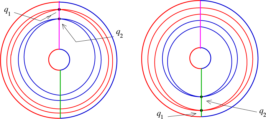
, respectively. Figure 11 displays the feature of a vector field
 $X \in {\mathcal H}^1$
. It is well known that a homoclinic connection corresponds to a codimension
 $1$
phenomenon, as expressed in the following.
Lemma 4.11. The subsets
 ${\mathcal H}^i$
are codimension
 $1$
submanifolds of
 ${\mathcal O}_1$
.
(a)
 $ q_1 \in \gamma _+^s$
implying that
 $X \in {\mathcal H}^1_+ $
and (b)
 $ q_1 \in \gamma _-^s$
implying that
 $X \in {\mathcal H}^1_- $
.

The submanifolds
 ${\mathcal H}^1$
and
 ${\mathcal H}^2$
cut
 ${\mathcal O}_\varphi $
into
 $4$
regions
 ${\mathcal O}_\varphi ^{\omega _1,\omega _2}$
,
 $\omega _i\in \{+,-\}$
, so that
 ${\omega _i=-}$
if and only if
 $q_i\in \Sigma ^i$
. Then we have the following lemma.
Lemma 4.12. Let X be a vector field in
 ${\mathcal O}_\varphi $
out of
 ${\mathcal H}^1$
and
 ${\mathcal H}^2$
. Then the first return map P admits a fixed point in
 $\Sigma ^1$
(respectively
 $\Sigma ^2$
) if and only if X belongs to
 ${\mathcal O}_\varphi ^{+,-}\cup {\mathcal O}_\varphi ^{+,+}$
(respectively
 ${\mathcal O}_\varphi ^{-,+}\cup {\mathcal O}_\varphi ^{+,+}$
).
Proof. If
 $q_1\in \Sigma ^2$
, it means that the cuspidal point of the pinched annulus
 $P(\Sigma ^1)$
belongs to
 $\Sigma ^2$
. Thus,
 $P(\Sigma ^1)$
crosses
 $\Sigma ^1$
in a hyperbolic way:
 $\Sigma ^1$
is a rectangle with a stable boundary
 $\gamma ^s_\pm $
and its image
 $P(\Sigma ^1)$
crosses completely
 $\Sigma ^1$
along a sub-rectangle with a stable side contained in each of
 $\gamma ^s_\pm $
, leading to a unique fixed point in
 $\Sigma ^1$
, see Figure 12(a). If
 $q_1\in \Sigma ^1$
, then
 $\Sigma ^1\cap P(\Sigma ^1)$
has two connected components which are cuspidal triangles
 $T_1^+$
(bounded by
 $\gamma ^s_+$
),
 $T_1^-$
(bounded by
 $\gamma ^s_-$
). Assume that there is a fixed point p in
 $T_1^-$
(for instance, the other case being equivalent). Then the region R bounded by
 $\gamma ^s_+$
and
 $W^s(p)$
is invariant by P, see Figure 12(b). However,
 $W^u(p)$
contains a segment joining p to
 $\gamma ^s_+$
. This segment is expanded by P, contradicting the invariance of R. This ends the proof.
 $ p_1$
and
 $p_2$
are fixed points of
 $X \in {\mathcal O}_{\varphi }\setminus {\mathcal H}^{1}\cup {\mathcal H}^{2}$
.

Consider now the region
 ${\mathcal O}_\varphi ^{+,+}$
: every vector field
 $X\in {\mathcal O}_\varphi ^{+,+}$
has exactly one fixed point
 $p_1$
in
 $\Sigma ^1$
and one fixed point
 $p_2$
in
 $\Sigma ^2$
. Let
 $W^s_i$
be the stable leaf through
 $p_i$
. Note that
 $q_1$
and
 $p_2$
are both in
 $\Sigma ^2$
and in the same way,
 $q_2$
and
 $p_1$
are both in
 $\Sigma ^1$
. This remark allows, a priori, that
 $q_1$
and
 $p_2$
belong to the same stable leaf or that
 $q_2$
and
 $p_1$
belong to the same stable leaf. This corresponds to our next splitting of the region
 ${\mathcal O}_\varphi ^{+,+}$
. Let us denote
 ${\mathcal H}{\mathcal E}_i$
as the subset of
 ${\mathcal O}_\varphi ^{+,+}$
corresponding to the vector fields X for which
 $q_i\in W^s_j$
. In other words, for
 $X\in {\mathcal H}{\mathcal E}_i$
, the unstable separatrix of
 $\sigma $
corresponding to
 $q_i$
is a heteroclinic connection with
 $p_j$
, see Figure 13. As in Lemma 4.11, one has the following lemma.
(a)
 $X \in {\mathcal H}{\mathcal E}_{1}$
and (b)
 $X \in {\mathcal H}{\mathcal E}_{2}$
.

Lemma 4.13. The subsets
 ${\mathcal H}{\mathcal E}_i$
are codimension
 $1$
submanifolds of
 ${\mathcal O}_\varphi $
.
Consider
 $X\in {\mathcal O}_\varphi ^{+,+}\setminus ({\mathcal H}{\mathcal E}_1\cup {\mathcal H}{\mathcal E}_2)$
. Then
 $\Sigma \setminus (W^s_1\cup W^s_2)$
has exactly two connected components: one, denoted by
 $\Sigma _+$
, contains
 $\gamma ^s_+$
, and the other, denoted by
 $\Sigma _-$
, contains
 $\gamma ^s_-$
. We denote by
 ${\mathcal L}^+$
the open subset of
 ${\mathcal O}_\varphi ^{+,+}$
where both points
 $q_1,q_2$
belong to
 $\Sigma _+$
and
 ${\mathcal L}^-$
the open set where both points
 $q_1,q_2$
belong to
 $\Sigma _-$
. We denote by
 $\widetilde {{\mathcal O}_\varphi }^{+,+}$
the open subset where
 $q_1$
and
 $q_2$
belong to different components
 $\Sigma _\pm $
and
 $\Sigma _\mp $
. We will denote
 ${\mathcal L}^{+,-}$
as the union
 $$ \begin{align*} {\mathcal L}^{+,-}={\mathcal O}_\varphi^{-,-}\cup {\mathcal O}_\varphi^{+,-}\cup{\mathcal O}_\varphi^{-,+}\cup\widetilde{{\mathcal O}_\varphi}^{+,+}\cup (({\mathcal H}^1\cup{\mathcal H}^2)\setminus (({\mathcal H}^1_+\cap {\mathcal H}^2_+) \cup ({\mathcal H}^1_-\cap {\mathcal H}^2_-)). \end{align*} $$
Recall that
 ${\mathcal H}^i$
corresponds to a homoclinic loop and
 ${\mathcal H}^i_\pm $
distinguishes the up or down connected components of
 $W^{s}(\sigma )\setminus W^{ss}(\sigma )$
involved in that loop.
5 The topological dynamics in the different regions of
${\mathcal O}_\varphi $

5.1 Upper- and down-Lorenz attractor: the regions
${\mathcal L}^+$
and
${\mathcal L}^-$


This section aims to prove the following result.
Theorem A. With the notation of §4.4, any vector field
 $X\in {\mathcal L}^+$
admits precisely two chain recurrence classes: one is an upper-Lorenz attractor and the other is a basic hyperbolic set, topologically equivalent to the suspension of a fake horseshoe. The symmetric statement holds in
 ${\mathcal L}^-$
, interchanging the up and down.
Proof. The component
 $\Sigma _+$
is a rectangle. The stable leaf
 $\gamma ^s_+$
cuts
 $\Sigma _+$
into two components. One is
 $\Sigma ^1\cap \Sigma _+$
and is bounded by
 $W^s_1=W^s(p_1)$
and the other is
 $\Sigma ^2\cap \Sigma _+$
and is bounded by
 $W^s_2$
. Note that
 $q_1$
belongs to
 $\Sigma ^2\cap \Sigma _+$
and
 $q_2$
belongs to
 $\Sigma ^1\cap \Sigma _+$
. Consider a stable leaf
 $L_1\in \Sigma ^1\cap \Sigma _+$
separating
 $W^s_1$
from
 $q_2$
, and a stable leaf
 $L_2\in \Sigma ^2\cap \Sigma _+$
separating
 $W^s_2$
from
 $q_1$
, see Figure 14. Then
 $L_1\cup L_2$
cuts
 $\Sigma ^+$
into three components: one is bounded by
 $W^s_1$
another by
 $W^s_2$
and the third, denoted by
 $R_L$
, is a rectangle bounded by both
 $L_1$
and
 $L_2$
and containing
 $q_2,q_1$
and
 $\gamma ^s_+$
. The leaf
 $\gamma ^s_+$
cuts
 $R_L$
in two components,
 $R_{L,1}\subset \Sigma _1$
and
 $R_{L_2}\subset \Sigma _2$
.
The leaves
 $L_1$
and
 $L_2$
, and the region
 $\Sigma _+$
.

Consider the restriction of P to
 $R_L\setminus \gamma ^+_s$
. The images of
 $R_{L_1}$
and
 $R_{L_2}$
are cuspidal triangles with cusps at
 $q_1$
and
 $q_2$
, and are contained in
 $R_L$
. Recall that P is hyperbolic. Thus, the restriction of P to
 $R_L$
satisfies all the properties of the return map in the geometric model of the Lorenz attractor with a rate expansion larger than
 $\varphi>\sqrt 2$
. The rectangle
 $R_L$
is an attracting region for P. One deduces that U contains an attracting sub-region, in which X is a geometric model of the Lorenz attractor.
Consider now the component
 $R_H$
of
 $\Sigma \setminus (L_1\cup L_2)$
disjoint from
 $R_L$
, and containing
 $\gamma ^s_-$
. Consider the restriction of P to
 $R_H\setminus \gamma ^s_-$
. The image of each of these components crosses
 $R_H$
in a Markovian way. Thus, the maximal invariant in
 $R_H$
is far from the discontinuity and is conjugated to the fake horseshoe, as the map P preserves the orientation of the unstable cone field. This ends the proof. The down case is similar.
5.2 Two-sided Lorenz attractor in
${\mathcal O}_\varphi ^{-,-}$

Proposition 5.1. For any
 $X\in {\mathcal O}_{\varphi }^{-,-}$
, the maximal invariant set in U is transitive and consists of a two-sided Lorenz attractor.
Proof. According to Lemma 4.9, for proving the transitivity of the maximal invariant, it is enough to verify that the iterates of an unstable segment S in
 $\Sigma $
cut all the stable leaves with the possible exception of a set with an empty interior, see Figure 15.
 $q_1 \in \Sigma ^1$
and
 $q_2 \in \Sigma ^2$
.

So consider an unstable segment
 $S\subset \Sigma $
. Consider the set of lengths of the connected components of all positive iterates
 $P^n(S)$
. If this set of lengths is not bounded, some component cuts every stable leaf, and we are done. Otherwise, given any
 $\delta>1$
, up to replace S by a segment in one of its iterates, one may assume that any connected component
 $S'$
in any iterate
 $P^n(S)$
has a length bounded by
 $\delta \ell (S)$
. We now fix
 $\delta \in ]1,{\unicode{x3bb} ^2}/2[$
.
If S is disjoint from
 $\gamma ^s_+\cup \gamma ^s_-$
, then
 $\ell (P(S))>\unicode{x3bb} \ell (S)>\delta \ell (S)$
contradicts the choice of S. So S cuts
 $\gamma ^s_+$
or
 $\gamma ^s_-$
. If it cuts both, then it crosses completely
 $\Sigma ^1$
or
 $\Sigma ^2$
so that
 $P(S)$
cuts all the stable leaves but one, and we are done. So we may assume that S cuts exactly one of
 $\gamma ^s_+$
or
 $\gamma ^s_-$
, say
 $\gamma ^s_+$
, for instance. Let
 $S_1$
be a component of
 $S\setminus \gamma ^s_+$
with a length larger or equal to
 $\frac 12\ell (S)$
. The length of
 $P(S_1)$
is at least
 $(\unicode{x3bb} /2) \ell (S)$
.
If
 $P(S_1)$
is disjoint from
 $\gamma ^s_+\cup \gamma ^s_-$
, then
 $$ \begin{align*} \ell(P(S_1)>\unicode{x3bb} \ell(S_1)> \frac{\unicode{x3bb}^2}2\ell(S)> \delta\ell(S), \end{align*} $$
contradicting the choice of S. So
 $P(S_1)$
cuts
 $\gamma ^s_+$
or
 $\gamma ^s_-$
. Once again, if it cuts both of them, we are done, so one may assume that
 $P(S_1)$
cuts exactly one of
 $\gamma ^s_+$
or
 $\gamma ^s_-$
. Note that one of the endpoints of
 $P(S_1)$
is a cuspidal point
 $q_i\in \Sigma ^i$
as
 $X\in {\mathcal O}_1^{-,-}$
. Thus, Lemma 4.7 applies and concludes the proof of the transitivity of the maximal invariant set
 $\Lambda _X$
. Note that the compact set
 $\Lambda _P$
consists of a union of essential circles in
 $\Sigma $
and therefore always cuts
 $\gamma ^s_+$
and
 $\gamma ^s_-$
, so that the maximal invariant set
 $\Lambda _X$
intersects non-trivially both stable sets
 $W^s_+(\sigma )$
and
 $W^s_-(\sigma )$
. Thus,
 $\Lambda _X$
is a two-sided Lorenz attractor, ending the proof. See Figure 15.
5.3 Two-sided Lorenz attractor in
${\mathcal O}^{+,-}_\varphi $
and
${\mathcal O}^{-,+}_{\varphi }$


Proposition 5.2. For any
 $X\in {\mathcal O}_{\varphi }^{+,-}\cup {\mathcal O}_{\varphi }^{-,+}$
, the maximal invariant set in U is transitive and consists of a two-sided Lorenz attractor.
The proof of the proposition for
 $X\in {\mathcal O}_{\varphi }^{-,+}$
is identical to the proof for
 $X\in {\mathcal O}_{\varphi }^{+,-} $
interchanging the components
 $\Sigma ^1$
and
 $\Sigma ^2$
, so we will write the proof only for
 $X\in {\mathcal O}_{\varphi }^{+,-}$
. See Figure 16.
 $q_1, q_2 \in \Sigma ^2$
for
 $X\in {\mathcal O}^{-,+}$
.

Proof. Recall that the rate of expansion of X is
 $\unicode{x3bb}>\varphi $
.
As for Proposition 5.1, it is enough to prove that the iterates of an unstable segment S in
 $\Sigma $
cut all the stable leaves with a possible exception of a set with an empty interior. See Figure 16. So consider an unstable segment
 $S\subset \Sigma $
. Consider the set of lengths of the connected components of all positive iterates
 $P^n(S)$
. If this set of lengths is not bounded, some component cuts every stable leaf, and we are done. Otherwise, given any
 $\delta>1$
, up to replace S by a segment in one of its iterates, one may assume that any connected component
 $S'$
in any iterate
 $P^n(S)$
has a length bounded by
 $\delta \ell (S)$
. We now fix
 $\delta \in ]1,{\unicode{x3bb} }/\varphi [$
.
If S is disjoint from
 $\gamma ^s_+\cup \gamma ^s_-$
, then
 $\ell (P(S)>\unicode{x3bb} \ell (S)>\delta \ell (S)$
contradicts the choice of S. So S cuts
 $\gamma ^s_+$
or
 $\gamma ^s_-$
. If it cuts both, then it crosses completely
 $\Sigma ^1$
or
 $\Sigma ^2$
so that
 $P(S)$
cuts all the stable leaves but one, and we are done.
So we may assume that S cuts exactly one of
 $\gamma ^s_+$
or
 $\gamma ^s_-$
, say
 $\gamma ^s_-$
, for instance. Thus, S is cut by
 $\gamma ^s_-$
into two components
 $S_i=S\cap \Sigma ^i$
. Consider
 $P(S_2)$
. If
 $P(S_2)\cap (\gamma ^s_-\cup \gamma ^s_+)\neq \emptyset $
, then Lemma 4.7 applies (because
 $q_2\in \Sigma ^2$
by our assumption
 $X\in {\mathcal O}^{+,-}_\varphi $
). Thus, the iterate of
 $S_2$
cuts every stable leaf but a finite number of them so that we are done.
Thus, we may assume that
 $P(S_2)$
is disjoint from
 $\gamma ^s_-\cup \gamma ^s_+$
. Hence,
 $P(S_2)$
is an unstable segment of length larger than
 $\unicode{x3bb} ^2\ell (S_2)$
. However,
 $\ell (P(S_1))\geq \unicode{x3bb} \ell (S_1)$
. Now Lemma 4.10 implies that
 $\max \{\ell (P(S_1)),\ell (P^2(S_2))\}\geq (\unicode{x3bb} /\varphi ) \ell (S)>\delta \ell (S)$
, contradicting the choice of the segment S, finishing the proof.
5.4 Two-sided Lorenz attractor in
$\widetilde {{\mathcal O}_\varphi }^{+,+}$

Proposition 5.3. For any
 $X\in \widetilde {{\mathcal O}_{\varphi }}^{+,+}$
, the maximal invariant set in U is transitive and consists of a two-sided Lorenz attractor.
Vector fields X in
 $\widetilde {{\mathcal O}_\varphi }^{+,+}$
are characterized by the fact that the points
 $q_1$
and
 $q_2$
belong to different components
 $\Sigma _+$
(containing
 $\gamma ^s_+$
) and
 $\Sigma _-$
(containing
 $\gamma ^s_-$
) of
 $\Sigma \setminus (W^s_1\cup W^s_2)$
, where
 $W^s_i=W^s(p_i)$
and
 $p_i$
is the fixed point of P in
 $\Sigma ^i$
. Thus,
 $\widetilde {{\mathcal O}_\varphi }^{+,+}$
is the union of two disjoint open subsets, defined by
 $q_1\in \Sigma _+$
or
 $q_1\in \Sigma _-$
. The proof of the proposition is symmetrical in these two open sets. We provide here the proof where
 $q_1\in \Sigma _+$
. See Figure 17.
 $q_1 \in \Sigma _+$
for
 $X\in \widetilde {{\mathcal O}_\varphi }^{+,+}$
.

Proof. Most of the proof is identical to the proofs of Propositions 5.1 and 5.2, and allows us to consider a segment S so that any component in any iterate
 $P^n(S)$
has a length bounded by
 $\delta \ell (S)$
with
 $1<\delta <\unicode{x3bb} /\varphi $
, where
 $\unicode{x3bb} $
is the expansion rate of X. Furthermore, S cuts exactly one of the stable leaves
 $\gamma ^s_+$
or
 $\gamma ^s_-$
. Let us assume that S cuts
 $\gamma ^s_-$
, and denote
 $S_i=S\cap \Sigma _i$
. If one of
 $P(S_1)$
or
 $P(S_2)$
is disjoint from
 $\gamma ^s_+ \cup \gamma ^s_-$
, then one concludes in the same way as in the proof of Proposition 5.2 that, using Lemma 4.10, one of the iterates
 $P(S_1)$
,
 $P^2(S_1)$
,
 $P(S_2)$
, or
 $P^2(S_2)$
contains a segment of length larger than
 $\unicode{x3bb} /\varphi $
contradicting the choice of S. Thus, one may assume that both
 $P(S_1)$
and
 $P(S_2)$
cut
 $\gamma ^s_+ \cup \gamma ^s_-$
. For the orientation of
 ${\mathcal C}^u$
,
 $S_1$
has its endpoint at
 $\gamma ^s_-$
. Thus,
 $P(S_1)$
ends at
 $q_1\in \Sigma _+$
. As seen above,
 $P(S_1)$
cuts
 $\gamma ^s_+ \cup \gamma ^s_-$
and its orientation implies that indeed it cuts
 $\gamma ^s_-$
. In particular, it goes out of
 $\Sigma _+$
. One deduces that
 $P(S_1)$
cuts transversely
 $W^s_2=W^s(p_2)$
, where
 $p_2$
is the fixed point in
 $\Sigma _2$
(recall that
 $X\in {\mathcal O}_\varphi ^{+,+}$
). Thus, Lemma 4.9 ensures that the iterates of
 $P(S_2)$
cross all stable leaves but a finite number of them, concluding that case.
The case where S cuts
 $\gamma ^s_+$
is similar, just replacing
 $S_1=S\cap \Sigma _1$
and
 $W^s(p_2)$
by
 ${S_2=S\cap \Sigma _2}$
and
 $W^s(p_1)$
. This concludes the proof.
5.5 Two-sided Lorenz attractor in hypersurfaces
${\mathcal H}^i$
of homoclinic loops

Theorem B. For any
 $X\in {\mathcal O}_1$
in one of the hypersurfaces
 ${\mathcal H}^1$
or
 ${\mathcal H}^2$
, the maximal invariant in U is a transitive singular attractor meeting both stable sets
 $W^s_\pm (\sigma )$
.
Proof. We assume that one of the points
 $q_1,q_2$
, say
 $q_1$
, belongs to one of the stable leaves
 $\gamma ^s_+$
or
 $\gamma ^s_-$
, say
 $q_1\in \gamma ^s_+$
(all the cases admit an identical proof, mutatis mutandis). See Figure 18.
 $X \in {\mathcal H}^1 \cup {\mathcal H}^2$
.

Similarly to the proof of Propositions 5.1, 5.2, and 5.3, the proof consists in considering an unstable segment S which does not admit any segment
 $\tilde S$
of length larger than
 $\delta \ell (S)$
,
 $1<\delta <\unicode{x3bb} /\varphi $
, so that
 $\tilde S$
, excepted a finite subset, is contained in the union of the iterate
 $P^n(S)$
,
 $n\geq 0$
. One needs to prove that the iterates of such a segment S cut any stable leaves but a finite number of them. Again, the choice of S implies that S cuts
 $\gamma ^s_+$
or
 $\gamma ^s_-$
, and if it cuts both, then
 $P(S)$
already cuts all stable leaves but one. So we assume that S cuts only one of these leaves.
Assume first that S cuts
 $\gamma ^s_+$
. Consider
 $S_1=S\cap \Sigma ^1$
. It is a segment starting at a point in
 $\gamma ^s_+$
and contained in
 $\Sigma ^1$
. Then
 $P(S_1)$
is a segment a length larger than
 $\unicode{x3bb} \ell (S)$
and starting at
 $q_1\in \gamma ^s_+$
. If
 $P(S_1)$
is not included in
 $\Sigma ^1 $
, then it cuts both
 $\gamma ^s_+$
and
 $\gamma ^s_-$
, and
 $P^2(S_1)$
cuts all leaves but one. If
 $P(S^1)\subset \Sigma ^1$
, then
 $P^2(S_1)$
is a segment of length larger than
 $\unicode{x3bb} ^2\ell (S)$
and starting at
 $q_1$
. Iterating the process, one gets that one of the iterates
 $P^k(S_1)$
crosses completely
 $\Sigma ^1$
so that
 $P^{k+1}(S_1)$
cuts all stable leaves but one, and we are done.
Assume now that S cuts
 $\gamma ^s_-$
. Consider
 $S_i=S\cap \Sigma ^i$
. Then
 $P(S_1)$
is a segment ending at
 $q_1\in \gamma ^s_+$
, and
 $P(S_1)$
either crosses completely
 $\Sigma ^2$
(and we are done) or is contained in
 $\Sigma ^2$
. Now
 $P^2(S_1)$
is a segment ending at
 $q_2$
. However,
 $P(S_2)$
is a segment starting at
 $q_2$
. Now
 $P^2(S_1)\cup \{q_2\}\cup P(S_2)$
is a segment of length at least
 $\unicode{x3bb} \ell (S)$
. This contradicts the choice of S, ending the proof.
The statement of Theorem B does not announce a two-sided Lorenz attractor, because the
 ${\mathcal H}^i$
are not open subsets, and then the robustness of the transitivity is not ensured. However, we will see below that
 $X\in {\mathcal H}^i$
exhibits indeed a two-sided Lorenz attractor excepted for X in a codimension
 $2$
submanifold. Let
 ${\mathcal H}^{1,2}_+$
and
 ${\mathcal H}^{1,2}_-$
be the codimension
 $2$
submanifolds included in
 ${\mathcal H}^1\cup {\mathcal H}^2$
consisting in vector fields X so that
 $q_1,q_2\in \gamma ^s_+$
or
 $q_1,q_2\in \gamma ^s_-$
, respectively, see Figure 19. Thus, both unstable separatrices of
 $\sigma $
are homoclinic connections and are included in the same connected component of
 $W^s(\sigma )\setminus W^{ss}(\sigma )$
.
 $ X \in {\mathcal H}^1\cup {\mathcal H}^2$
, and
 $q_1,q_2\in \gamma ^s_+$
and
 $q_1,q_2\in \gamma ^s_-$
.

The next lemma ensures that for
 $X\in {\mathcal H}^i$
out of
 ${\mathcal H}^{1,2}_+$
and
 ${\mathcal H}^{1,2}_-$
, the transitivity of the attractor is robust so that the attractor is a two-sided Lorenz attractor.
Theorem C. If
 $X\in {\mathcal H}^i\setminus ({\mathcal H}^{1,2}_+ \cup {\mathcal H}^{1,2}_-)$
, there is a neighborhood
 ${\mathcal U}(X)$
of X such that the maximal invariant set for every
 $Y\in {\mathcal U}(X)$
is a two-sided Lorenz attractor.
Proof. The proof consists of unfolding the homoclinic loops and checking that all the possibilities lead to one of the
 ${\mathcal O}^{-,-}_\varphi \cup {\mathcal O}^{+,-}_\varphi \cup {\mathcal O}^{-,+}_\varphi \cup \widetilde {{\mathcal O}^{+,+}_\varphi }\cup {\mathcal H}^1\cup {\mathcal H}^2$
.
5.6 Two-sided Lorenz attractor in
${\mathcal L}^{+-}$

Note that Propositions 5.1, 5.2, 5.3, and B and Lemma C together prove the following theorem.
Theorem D. For any
 $X\in {\mathcal L}^{+,-}$
, the maximal invariant set in U is a transitive singular hyperbolic attractor meeting both stable sets
 $W^{s}_{-}(\sigma )$
and
 $W^s_{+}(\sigma )$
; that is, it is a two-sided Lorenz attractor.
The region
 ${\mathcal L}^{+,-}$
has been defined as a union of many regions, and the propositions listed above prove the conclusion of Proposition D in each of these regions. Finally, some of these regions are not open, so Lemma C checks that the vector fields in these non-open regions admit neighborhoods contained in the union of the other regions.
5.7 The collisions of the Lorenz attractor and a fake horseshoe: vector fields in
${\mathcal H}{\mathcal E}_i$

In this section, we consider vector fields X in
 ${\mathcal O}^{+,+}_\varphi $
, that is, so that the return map P has two fixed points
 $p_i\in \Sigma ^i$
,
 $i=1,2$
, a heteroclinic connection between
 $\sigma $
and one of the points
 $p_i$
. More precisely,
 $q_i$
belongs to the stable leaf
 $W^s_j$
through
 $p_j$
; note that
 $j\neq i$
because
 $q_i$
is not in
 $\Sigma ^i$
when
 $\Sigma ^i$
contains a fixed point. The case when both
 $q_1$
and
 $q_2$
belong to
 $W^s_1\cup W^s_2$
corresponds to
 $X\in {\mathcal H}{\mathcal E}_1\cap {\mathcal H}{\mathcal E}_2$
, which is a codimension
 $2$
submanifold.
Theorem E. For any
 $X\in {\mathcal H}{\mathcal E}_1\cap {\mathcal H}{\mathcal E}_2$
, there is a unique chain recurrence class, which is not transitive. Both
 $\Sigma _-$
and
 $\Sigma _+$
are invariant by P. The maximal invariant set of the restriction of P to
 $\Sigma _i$
is transitive: every unstable segment in
 $\Sigma _i$
has its iterates which cut every segment in
 $\Sigma _i$
. The attracting set U splits into
 $2$
connected compact sets, each containing a full Lorenz intersecting along
 $W^s(p_1)\cup W^s(p_2)\cup W^u(\sigma )$
.
Proof. The first return map is illustrated in Figure 20. The study of the first return map in each rectangle
 $\overline \Sigma _i$
is classical for the expansion rate larger than
 $\sqrt 2<\varphi $
.
 $X\in {\mathcal H}{\mathcal E}_1\cap {\mathcal H}{\mathcal E}_2$
.

The submanifold
 ${\mathcal H}{\mathcal E}_1\cap {\mathcal H}{\mathcal E}_2$
cuts
 ${\mathcal H}{\mathcal E}_1$
into two (relative) open subsets, as
 $q_2$
belongs either to
 $\Sigma _+$
or
 $\Sigma _-$
(connected components of
 $\Sigma \setminus (W^s_1\cup W^s_2)$
. In the same way, the submanifold
 ${\mathcal H}{\mathcal E}_2\cap {\mathcal H}{\mathcal E}_2$
cuts
 ${\mathcal H}{\mathcal E}_2$
into two (relative) open subsets, as
 $q_1$
belongs either to
 $\Sigma _+$
or
 $\Sigma _-$
(connected components of
 $\Sigma \setminus (W^s_1\cup W^s_2)$
.
We will consider
 $X\in {\mathcal H}{\mathcal E}_1\setminus ({\mathcal H}{\mathcal E}_1\cap {\mathcal H}{\mathcal E}_2)$
, and
 $q_2\in \Sigma _+$
, the other cases are similar.
Then the stable leaf through
 $q_2$
cuts
 $\Sigma _+$
into two components, one, denoted as
 $\Sigma ^+_1$
, bounded by the stable leaf
 $W^s_1$
through
 $p_1$
and the other, denoted as
 $\Sigma ^+_2$
, bounded by
 $W^s_2$
(which contains
 $q_1$
by definition of
 ${\mathcal H}{\mathcal E}_1$
); notice that
 $\Sigma ^+_2$
contains the stable leaf
 $\gamma ^s_+$
, because
 $q_2\in \Sigma ^1$
. Note that if
 $X\in {\mathcal H}{\mathcal E}_1\setminus ({\mathcal H}{\mathcal E}_1\cap {\mathcal H}{\mathcal E}_2)$
, then
 $q_1\in W^s(p_2)$
and
 ${q_2 \notin W^s(p_1)}$
.
Proposition 5.4. Consider
 $X\in {\mathcal H}{\mathcal E}_1\setminus ({\mathcal H}{\mathcal E}_1\cap {\mathcal H}{\mathcal E}_2)$
, and assume
 $q_2\in \Sigma _+$
. Then we have the following.
-
• X has a unique chain recurrence class in U, but this class is not transitive and consists of two (singular) homoclinic classes
$K_-,K_+$
containing
$\sigma $
. -
• The iterates by P of any unstable segment in
$\Sigma $
cut any stable leaf in
$\Sigma ^+_2$
but finitely many of them. Furthermore, the return map P restricted to the rectangle
$\overline {\Sigma ^+_2}$
is a Lorenz map for the parameter corresponding to one homoclinic connection. See Figure 21.
Figure 21The left diagram displays
$P(\Sigma )$
for
$X\in {\mathcal H}{\mathcal E}_1\setminus ({\mathcal H}{\mathcal E}_1\cap {\mathcal H}{\mathcal E}_2)$
and
$q_2\in \Sigma _2^+$
. The middle diagram displays the restriction of
$P|_{\Sigma ^+_2}$
and the right diagram displays the restriction of P to
$\Sigma \setminus \Sigma ^+_2$
.Figure 22The maximal invariant set in U of
$X \in {\mathcal H}^{1,2}_+ \cup {\mathcal H}^{1,2}_-$
is a fat Lorenz. -
• The homoclinic class
$K_-$
is a singular fake horseshoe that intersects
$\Sigma _-$
and is disjoint from
$\Sigma _+$
. -
• The intersection
$K_-\cap K_+\cap \Sigma $
is contained in
$W^s_2$
and consists of
$p_2$
and the orbit of
$q_1$
.


Proof. We refer the reader to the pictures illustrating the restriction of the return map P to
 $\Sigma ^+_2$
and to
 $\Sigma \setminus \Sigma ^+_2$
. See Figure 21.
A similar result holds for
 $X \in \mathcal {HE}_{i} \setminus (\mathcal {HE}_1 \cap \mathcal {HE}_2)$
and
 $q_i \in \Sigma _j$
,
 $i \in \{1,2\}$
and
 ${j \in \{-,+\}}$
.
5.8 Fat Lorenz attractor: vector fields in
${\mathcal H}^{1,2}_+$
and
${\mathcal H}^{1,2}_-$


We start this section setting the concept of ‘fat Lorenz attractor’.
Definition 5.5. Consider a vector field
 $X\in {\mathcal O}_\varphi $
and
 $\Lambda $
its maximal invariant (compact) set in U. We say that
 $\Lambda $
is a fat Lorenz attractor if every unstable segment in
 $\Sigma \setminus \gamma ^s_+$
(respectively
 $\Sigma \setminus \gamma ^s_-$
) has an iterate by P which cuts every stable leaf excepted
 $\gamma ^s_+$
(respectively
 $\gamma ^s_-$
), see Figure 22.
Notice that Definition 5.5 implies that
 $\Lambda $
is a transitive attractor.
Proposition 5.6. If
 $X\in {\mathcal H}^{1,2}_+$
(respectively
 $X\in {\mathcal H}^{1,2}_-$
), then the maximal invariant set in U is a fat Lorenz attractor.
6 Collisions and collapses
This section describes the drastic changes of behavior appearing in the topological dynamics when a family
 $X_\mu $
crosses the boundary of the regions we described in §5.
6.1 Collisions
Let us consider a 1-parameter family
 $X_\mu \in {\mathcal O}^{+,+}_\varphi $
,
 $\mu \in [-1,1]$
with the following properties.
-
• The family crosses the hypersurface transversely
${\mathcal H}{\mathcal E}^1_+$
at
$\mu =0$
: this means that
$X_0$
exhibits a heteroclinic connection
$q_1\in W^s_2$
and
$q_2\in \Sigma _+$
. -
• For
$\mu <0$
, the vector field
$X_\mu $
belongs to
${\mathcal L}^+$
: it has an up Lorenz attractor and
$\Sigma _-$
contains a fake horseshoe for P. -
• For
$\mu>0$
, the vector field
$X_\mu $
has a two-sided Lorenz attractor.


In other words,
 $X_\mu $
consists of a generic unfolding of the heteroclinic connection
 ${q_1\in W^s_2}$
. The cuspidal point
 $q_{1,\mu }$
is moving with the parameter
 $\mu $
and is crossing transversely
 $W^s_{2,\mu }$
(stable leaf through
 $p_{2,\mu }$
) for
 $\mu =0$
. For
 $\mu <0$
, the upper-Lorenz attractor is intersecting exactly every stable leaf in
 $\Sigma ^+$
between
 $q_{2,\mu }$
and
 $q_{1,\mu }$
, and the horseshoe in
 $\Sigma _-$
is bounded by the stable leaves
 $W^s_{1,\mu }$
,
 $W^s_{2,\mu }$
and contains the periodic points
 $p_{1,\mu }$
 $p_{2,\mu }$
.
When
 $\mu $
tends to
 $0$
, the point
 $q_{1,\mu }$
tends to a point
 $q_{1,0}$
in
 $W^s_2$
, and this point
 $q_{1,0}$
is also the limit of the intersection of
 $W^s_2$
with one of the rectangles (the one containing
 $p_1$
) of the Markov partition of the fake horseshoe. This corresponds to a Cantor set in
 $W^s_2$
of points of the fake horseshoe for
 $X_\mu $
,
 $\mu <0$
whose diameter tends to
 $0$
as
 $\mu \to 0$
: all the Cantor set tends to
 $q_{1,0}$
.
For the parameter
 $0$
, the Lorenz attractor no longer admits an attracting neighborhood and is no longer robust. The fake horseshoe becomes singular, and intersects the Lorenz attractor along
 $\sigma $
and the orbits of
 $p_{2,0}$
and of
 $q_{1,0}$
. When
 $\mu>0$
, the Lorenz attractor and the (singular) fake horseshoe merge into a two-sided Lorenz attractor.
Notice that if all the vector fields
 $X_\mu $
are assumed to be of class
 $C^2$
, then all along the parameter,
 $X_\mu $
admits a unique Sinai–Ruelle–Bowen measure
 $\nu _\mu $
(see [Reference Araújo, Pacifico, Pujals and Viana11]). For
 $\mu \leq 0$
, the support of
 $\nu _\mu $
is the Lorenz attractor, and in particular, does not intersect
 $\Sigma _-$
. For
 $\mu>0$
, the support of
 $\nu _\mu $
intersects any stable leaf in
 $\Sigma $
. Thus, the support of
 $\nu _\mu $
changes drastically at the collision point.
Question 1. Is the map
 $\mu \mapsto \nu _\mu $
continuous (for the weak topology) at
 $\mu =0$
?
6.2 The collapse of the horseshoe: parameter families crossing
${\mathcal H}^{1,2}_+$
or
${\mathcal H}^{1,2}_-$


Recall that
 ${\mathcal H}^{1,2}_+$
is the codimension
 $2$
submanifold corresponding to the double homoclinic connection
 $q_1,q_2\in \gamma ^s_+$
. We consider here a
 $2$
-parameter family
 $X_{\mu }$
,
 $\mu =(\mu _1,\mu _2)\in [-1,1]^2$
which is a generic unfolding of this double homoclinic connection: in other words, the family cuts transversely
 ${\mathcal H}^{1,2}_+$
at
 $\mu =(0,0)$
. We assume furthermore that, for any fixed
 $\mu _2$
, the
 $1$
-parameter family
 $X_{\mu _1,\mu _2}$
is transverse to
 ${\mathcal H}^1$
at
 $\mu _1=0$
and, reciprocally, for any fixed
 $\mu _1$
, the
 $1$
-parameter family
 $X_{\mu _1,\mu _2}$
is transverse to
 ${\mathcal H}^1$
at
 $\mu _2=0$
. More precisely, one may assume that
 $X_{\mu _1,\mu _2}\in {\mathcal O}_\varphi ^{\omega _1,\omega _2}$
, where
 $\omega _i\in \{-,+\}$
is the sign of
 $\mu _i$
. When one unfolds this double homoclinic connection, if
 $q_{1,\mu }$
enters in
 $\Sigma _2$
(that is,
 $\mu _1>0$
), then a fixed point
 $p_{1,\mu }\in \Sigma _1$
is created and tends to
 $q_{1,0}\in \gamma ^s_+$
as
 $\mu $
tends to
 $0$
. In the same way, if
 $\mu _2>0$
, then
 $q_2$
enters in
 $\Sigma _1$
and the fixed point
 $p_{2,\mu }$
is created in
 $\Sigma _2$
and tends to
 $q_{2,0}\in \gamma ^s_+$
. The stable leaves
 $W^s_{1,\mu }$
and
 $W^s_{2,\mu }$
bound the small strip
 $\Sigma ^+$
in
 $\Sigma $
containing
 $\gamma ^s_+$
(tending to the segment
 $\gamma ^s_+$
as
 $\mu \to 0$
) and a large strip
 $\Sigma ^-$
. The vector field
 $X_\mu $
in
 ${\mathcal O}^{+,+}_\varphi $
belongs to
 ${\mathcal L}^+\cup {\mathcal L}^-$
if and only if both
 $q_1$
and
 $q_2$
belong to the same component
 $\Sigma ^+$
or
 $\Sigma ^-$
.
Lemma 6.1. For small
 $\mu $
,
 $\{q_1,q_2\}$
is not contained in
 $\Sigma ^+$
. In other words, the closure of
 ${\mathcal L}^+$
is disjoint from
 ${\mathcal H}^{1,2}_+$
. Here,
 $\{\mu |\{q_{1,\mu },q_{2,\mu } \}\subset \Sigma _-\}$
is an open subset containing
 $(0,0)$
in its closure. More precisely, for any
 $\alpha>0$
, there is
 $\mu _0$
so that for any
 $0<\mu <\mu _0$
, the vector field
 $X_{\mu ,\alpha \mu }\in {\mathcal L}^-.$
Proof. Assume (arguing by contradiction) that
 $\{q_1,q_2\}\subset \Sigma ^+$
. Thus,
 $X\in {\mathcal L}^+$
. Then
 $\Sigma ^+$
is invariant under the action of P. However, as
 $\Sigma ^+$
is contained in an arbitrarily small neighborhood of
 $\gamma ^s_+$
, the rate of expansion of P in the unstable cone is arbitrarily large, in particular,
 $\gg 2$
. So
 $\Sigma ^+$
cannot be invariant, ending the proof.
The proof of the second point is as follows: consider one half-line
 $X_{\mu ,\alpha \mu }$
and consider
 $\mu>0$
very small. Thus, the point
 $q_1$
(respectively
 $q_2$
) belongs to
 $\Sigma _2$
(respectively
 $\Sigma _1$
) and its distance to
 $\gamma ^s_+$
is
 $\mu $
(respectively
 $\alpha \mu $
). Consider any point p in
 $\Sigma _1$
at a small distance
 $>\frac 12\alpha \mu $
from
 $\gamma ^s_+$
. Consider an unstable segment
 $\gamma _p$
realizing this distance so that
 $\gamma _p$
starts at
 $\gamma ^s_+$
and ends at p. Then
 $P(\gamma _p)$
is an unstable segment starting at
 $q_1$
and ending at
 $P(p)$
. The length
 $\ell (P(\gamma _p))$
is arbitrarily larger than
 $\ell (\gamma _p)$
(say, larger than
 $100 (1+\alpha )\mu \ell (\gamma _p)$
as
 $\mu $
tends to
 $0$
(as the expansion rate close to
 $\gamma ^s_+$
tends to infinity).
One deduces that the point
 $P(p)$
belongs to
 $\Sigma _1$
and is at a distance larger than
 $ {99(1+\alpha )\mu} $
of
 $\gamma ^s_+$
. One deduces that
 $P(p)$
(and thus p) does not belong to the stable leaf through the fixed point
 $p_1\in \Sigma _1$
. In particular,
 $q_2$
belongs to
 $\Sigma _-$
. One proves in the same way as for
 $\mu>0$
small
 $q_1\in \Sigma _-$
, and thus the vector field belongs to
 ${\mathcal L}^-$
, ending the proof. Figure 4 displays a local bifurcation diagram in this case.
The lemma implies that when one considers a segment in the parameter plane crossing
 $(0,0)$
and entering in
 ${\mathcal O}^{+,+}_\varphi $
transversely to both
 ${\mathcal H}^1$
and
 ${\mathcal H}^2$
, then one creates a down-Lorenz attractor, which cuts every stable leaf in
 $\Sigma ^-$
. When the parameter tends to
 $(0,0)$
, then
 $\Sigma ^-$
tends to
 $\Sigma $
and the Lorenz attractor tends to what we call the fat Lorenz attractor. The horseshoe, corresponding to
 $\Sigma ^+$
, collapses into the double homoclinic connection.
6.3 Switching from upper to down: family crossing
${\mathcal H}{\mathcal E}_1\cap {\mathcal H}{\mathcal E}_2$

In this section, we consider a two-parameter family
 $X_\mu \in {\mathcal O}_\varphi ^{+,+}$
,
 $\mu =(\mu _1,\mu _2)$
crossing transversely
 ${{\mathcal H}{\mathcal E}_1\cap {\mathcal H}{\mathcal E}_2}$
at
 $\mu =0$
. In other words,
 $X_{(0,0)}$
exhibits two heteroclinic connections
 $q_1\in W^s_2$
and
 $q_2\in W^s_1$
(recall that
 $W^s_i$
is the stable leaf through the fixed point
 $p_i$
). We have seen that this behavior implies that
 $X_{(0,0)}$
has two full Lorenz which intersect along
 $W^s(p_1)\cup W^s(p_2)\cup W^u(\sigma )$
. See Figure 20. Up to reparameterization, the family one may assume that
 $$ \begin{align*}\begin{array}{c} (\mu_1=0 \Leftrightarrow q_1\in W^s_2) \quad\mbox{and}\quad (\mu_2=0 \Leftrightarrow q_2\in W^s_1),\\ (\mu_1>0 \Leftrightarrow q_1\in \Sigma^+) \quad\mbox{and}\quad (\mu_2>0 \Leftrightarrow q_2\in \Sigma^+). \end{array}\end{align*} $$
With these notation, note that Theorems F and G are a reformulation of the results in the previous sections. Figure 23 displays the local bifurcations.
Local bifurcation: (a)
 $(\mu _1,\mu _2), \mu _i>0$
; (b)
 $(\mu _1,\mu _2), \mu _i =0$
; (c)
 $(\mu _1,\mu _2), \mu _i < 0$
.

7 Parameter families
$X_\mu \in {\mathcal O}_\varphi $
, with parameters in the torus

7.1
${\mathbb T}^2$
-parameter families

Definition 7.1. Let
 $\pi \colon {\mathbb R}^2\to {\mathbb T}^2={\mathbb R}^2/{\mathbb Z}^2$
be the canonical projection. Let
 $V\subset {\mathbb R}^2$
be an open subset so that the projection
 $\pi (V)$
is the whole torus
 ${\mathbb T}^2$
. We say that a family
 $\{X_\mu \in {\mathcal O}_1\}_{\mu \in V}$
is a
 $C^r, r\geq 0,$
family of vector fields in
 ${\mathcal O}_1$
parameterized by
 ${\mathbb T}^2$
if:
-
• the map
$\mu \to X_\mu $
is continuous for the
$C^1$
-topology; -
• the map
$(p,\mu )\mapsto X_\mu (p)$
is of class
$C^r$
; -
• for any
$\mu ,\mu '$
so that
$\mu '-\mu \in {\mathbb Z}^2$
one has: the return maps
$P,P'$
of
$X,X'$
on the transverse cross-section
$\Sigma $
coincide:
$P=P'$
. In particular, the restriction of X and
$X'$
to the attracting region U are smoothly topologically equivalent, by an equivalence whose restriction to the cross-section
$\Sigma $
is the identity map.


Shortly, we say that
 $X_\mu $
is a
 ${\mathbb T}^2$
-parameter family.
7.2 Essential families
This section aims to define the notion of essential
 ${\mathbb T}^2$
families. Roughly, we do not want the family
 $X_\mu $
to be contained in a small neighborhood of a given vector field
 $X_0$
. We want that, when
 $\mu $
follows a simple closed path in
 ${\mathbb T}^2$
, non-homotopic to a point, then the images
 $P(\Sigma ^1)$
or
 $P(\Sigma ^2)$
give a turn in
 $\Sigma $
in an essential way.
Let us first present a non-intrinsic definition of these phenomena. Afterwards, we will see an intrinsic definition, showing that the definition does not depend on the choices. Consider a
 ${\mathbb T}^2$
-parameter family
 $\{X_\mu \}$
, and let
 $\gamma ^s_{+,\mu }$
and
 $\gamma ^s_{-,\mu }$
be the associated stable leaves corresponding to the discontinuities of the first return map. The leaves
 $\gamma ^s_{+, \mu }$
vary continuously with
 $\mu $
. This allows us to choose a parameterization of
 $\Sigma $
, depending on
 $\mu $
, and so that
 $\gamma ^s_{+,\mu }$
is the segment
 $\{0\}\times [-1,1]$
in the annulus
 $\Sigma ={\mathbb R}/{\mathbb Z}\times [-1,1]$
.
Consider now the points
 $q_{1,\mu }$
and
 $q_{2,\mu }$
(first intersection points of the unstable separatrices of
 $\sigma _\mu $
with
 $\Sigma $
). This defines two continuous maps
 $q_1\colon {\mathbb T}^2\to {\mathbb R} /{\mathbb Z}\times [-1,1] \mbox { and } q_2\colon {\mathbb T}^2\to {\mathbb R}/{\mathbb Z}\times [-1,1]$
. Then, composing
 $q_1$
and
 $q_2$
by the projection
 $\psi \colon {\mathbb S}^1\times [-1,1]\to {\mathbb S}^1$
, one gets two continuous maps
 $\psi \circ q_i\colon {\mathbb T}^2\to {\mathbb S}^1$
,
 $i=1,2$
.
 $\mbox {Let us denote}\quad Q=(\psi \circ q_1, \psi \circ q_2) \colon {\mathbb T}^2\to {\mathbb T}^2.$
Definition 7.2. With the notation above, we say that the family
 $X_\mu $
is essential if the topological degree of Q is
 $1$
(or else, if Q is homotopic to an orientation preserving homeomorphism).
In Definition 7.2, the homotopy class of Q depends on the parameterization of
 $\Sigma $
that we choose. Let us convince you that the topological degree of Q does not depend on the choice of parameterization of
 $\Sigma $
.
Consider the hypersurface
 $\Gamma ^s_+\subset \Sigma \times {\mathbb T}^2$
defined by
 $\Gamma ^s_+= \bigcup _{\mu } \gamma ^s_{+,\mu }\times \{\mu \}$
. In the parameterization above, it is
 $\{0\}\times [-1,1]\times {\mathbb T}^2\subset \Sigma \times {\mathbb T}^2$
. Thus, it is a compact
 $3$
-manifold with a boundary homeomorphic to
 $[-1,1]\times {\mathbb T}^2$
, whose boundary is contained in the boundary of
 $\Sigma \times {\mathbb T}^2$
. As a consequence, the algebraic intersection number of a closed curve in
 $\Sigma \times {\mathbb T}^2$
with
 $\Gamma ^s_+$
is well defined.
To every closed path
 $c\colon {\mathbb S}^1\to {\mathbb T}^2$
, let us consider the closed paths
 $q_{i,c}\colon {\mathbb S}^1\to \Sigma \times {\mathbb T}^2$
,
 $i\in \{1,2\}$
so that
 $q_{i,c}(\theta )= (q_{i,c(\theta )},c(\theta ))$
for
 $\theta \in {\mathbb S}^1$
.
Notice that
 $q_{i,c}$
depends continuously on the closed path c. In particular, its algebraic intersection number with the hypersurface
 $\Gamma ^s_+$
only depends on the homology class
 $[c]$
. We denote it by
 $[q_{i,c}]\cdot \Gamma ^s_+$
. One gets a map
 $$ \begin{align*}[c]\mapsto ([q_{1,c}]\cdot\Gamma^s_+,[q_{2,c}]\cdot\Gamma^s_+)\in{\mathbb Z}^2 \end{align*} $$
defined on
 $H_1({\mathbb T}^2,{\mathbb Z})\simeq {\mathbb Z}^2$
with values in
 ${\mathbb Z}^2$
, and this map is a linear map given by a
 $2$
by
 $2$
matrix with
 ${\mathbb Z}$
-entries. The topological degree of Q is the determinant of this linear map: the family is essential if and only if the determinant is
 $1$
, which does not depend on the parameterization choice.
7.3 Building
${\mathbb T}^2$
-families

Consider a vector field
 $X\in {\mathcal O}_1$
on
 $\mathbb {R}^3$
. Thus, by definition, it is transversal to the annuli
 $\Sigma $
,
 $D_1$
, and
 $D^2$
. Furthermore, the first return map
 $R\colon D_1\cup D_2\to \Sigma $
is smooth and maps
 $D_1$
and
 $D_2$
on two disjoint essential annuli in the interior of
 $\Sigma $
.
Consider an annuli
 $\tilde D_i$
,
 $i=1,2$
, containing
 $D_i$
in its interior, and so that R extends in a diffeomorphism
 $ \tilde R\colon \tilde D_1\cup \tilde D_2\to \Sigma $
, which is the first return map from
 $\tilde D_i$
to
 $\Sigma \cup \tilde D_1\cup \tilde D_2$
. We denote by
 $\Delta _i$
the union of the X-orbit segment joining points
 $p\in \tilde D_i$
to
 $\tilde R(p)$
. Thus,
 $(\Delta _i,X)$
is smoothly orbitally equivalent to
 $(\tilde D_i\times [0,1], \partial /{\partial t}).$
The next lemma expresses that one can realize by a continuous family of vector fields in
 $\mathbb {R}^3$
any continuous deformation of the return map R.
Lemma 7.3. Consider a continuous family
 $R_\mu \colon D_1\cup D_2\to \tilde R(\tilde D_1\cup \tilde D_2)$
,
 $\mu \in V$
, where
 $V\subset {\mathbb R}^2$
is an open disk containing
 $0$
. One assumes
 $R_0=R$
. Then there is a family of vector fields
 $X_\mu $
with the following properties:
-
•
$X_0=X$
; -
• for any
$\mu $
,
$X_\mu $
satisfies all the topological properties (items (1) to (7)) of the definition of the set
${\mathcal O}_1$
; -
• for any
$\mu $
,
$X_\mu $
coincides with X out of
$\Delta _1\cup \Delta _2$
; -
• for any
$\mu $
, the restriction of
$X_\mu $
to
$\Delta _i$
is transverse to the fibers
$\tilde D_i\times \{t\}$
; -
• the return map of X from
$D_1\cup D_2$
to
$\Sigma $
is
$R_\mu $
.


Proof. One extends
 $R_\mu $
to
 $\tilde D_i$
in a diffeomorphism
 $\tilde R_\mu $
so that all
 $\tilde R_\mu $
coincide with
 $\tilde R$
in a neighborhood of the boundary
 $\partial \tilde D_i$
. Then we replace the restriction of X in
 $\Delta _i$
with a vector field that coincides with X in a neighborhood of
 $\partial \Delta _i$
and where the entrance exit map is
 $\tilde R_\mu $
.
Assume now that the projection of V on
 ${\mathbb R}^2/{\mathbb T}^2$
covers the whole torus
 ${\mathbb T}^2$
, and assume that the family
 $R_\mu $
is
 ${\mathbb Z}^2$
-periodic in the following sense:
-
• for any
$\mu _1,\mu _2\in V$
so that
$\mu _2-\mu _1\in {\mathbb Z}^2$
, then
$R_{\mu _1}=R_{\mu _2}$
.


Then the family
 $X_\mu $
defined in Lemma 7.3 is a
 ${\mathbb T}^2$
-parameter family of vector fields having U as an attracting region.
7.4 An essential
${\mathbb T}^2$
-family of vector fields in
${\mathcal O}_\varphi $


Consider
 $\Sigma \simeq {\mathbb S}^1\times [-1,1]$
with the coordinates
 $\theta , t$
and consider the constant cone field
 ${\mathcal C}$
defined by
 $$ \begin{align*} {\mathcal C}(p)=\bigg\{u=\alpha\frac{\partial}{\partial \theta}+\beta\frac{\partial}{\partial t}\in T_p\Sigma \mbox{ so that } |\alpha|\geq |\beta|\bigg\}. \end{align*} $$
We denote by
 ${\mathcal R}_\alpha \colon \Sigma \to \Sigma $
the rotation of angle
 $\alpha \in {\mathbb S}^1$
, that is,
 $(\theta , t)\mapsto (\theta +\alpha ,t)$
. Recall that
 $R\colon D_1\cup D_2\to \Sigma $
is the first return map of
 $D_i$
to
 $\Sigma \cup D_1\cup D_2$
.
Consider a vector field
 $X\in {\mathcal O}_\varphi $
with the following extra properties.
-
• The constant cone field
${\mathcal C}$
is the unstable cone field
${\mathcal C}^u$
. -
• The images
$R(D_i)$
are product annulus
${\mathbb S}^1\times I_i \subset \Sigma ={\mathbb S}^1\times [-1,1]$
.


Now consider the
 ${\mathbb Z}^2$
-family of maps
 $R_{\alpha ,\beta }\colon D_1\cup D_2\to \Sigma $
,
 $\alpha ,\beta \in {\mathbb T}^2={\mathbb R}^2/{\mathbb S}^2$
defined by
 $$ \begin{align*} R={\mathcal R}_\alpha\circ R\mbox { on } D_1\quad \mbox{and}\quad R={\mathcal R}_\beta\circ R\mbox{ on } D_2. \end{align*} $$
According to Lemma 7.3, one can realize the periodic family
 $R_\mu $
by a
 ${\mathbb T}^2$
-parameter family of vector fields
 $X_\mu $
, and one can easily check.
Lemma 7.4. The family
 $X_\mu $
is a
 ${\mathbb T}^2$
-parameter essential family in
 ${\mathcal O}_\varphi $
.
8 Reduction to one-dimensional dynamics
8.1 The action of the return map on the space of stable leaves
Any
 $C^1$
vector field
 $X\in {\mathcal O}_1$
is singular hyperbolic in the attracting region U, with a continuous strong stable direction. There is a well-defined stable foliation (also called strong stable foliation) tangent to the stable distribution with leaves having the same regularity as X. It admits, therefore, a well-defined two-dimensional (weak)stable foliation (also called center-stable foliation) out of the strong stable manifold of the singularity. The leaves of the weak stable foliation are the orbits for the flow of the leaves of the strong stable one: out of the strong stable manifold of
 $\sigma $
, the vector is not tangent to the stable direction, so these orbits are two-dimensional. Along the strong stable manifold of
 $\sigma $
, the vector field is tangent to the one-dimensional strong stable leaf, so the foliation is singular. The strong stable foliation is not tangent to
 $\Sigma $
. However, the two-dimensional center-stable foliation cuts the annulus
 $\Sigma $
transversely along a one-dimensional foliation
 ${\mathcal F}^s$
, which is the stable foliation of the return map P. The segments
 $\gamma ^s_+$
and
 $\gamma ^s_-$
are leaves of
 ${\mathcal F}^s$
.
The foliation
 ${\mathcal F}^s$
is transverse to the unstable cone field
 ${\mathcal C}^u$
. The leaves of the foliation
 ${\mathcal F}^s$
are segments crossing
 $\Sigma $
(connecting the two boundary components of
 $\Sigma $
). The leaves space
 $\Sigma /{\mathcal F}^s$
is a (topological) circle
 ${\mathbb S}^1_X$
. The leaves
 $\gamma ^s_+$
and
 $\gamma ^s_-$
each induce a point
 $c_+$
and
 $c_-$
, respectively, on
 ${\mathbb S}^1_X$
. Note that the flow
 $X^t$
preserves the center-stable foliation, and thus the first return map P preserves the foliation
 ${\mathcal F}^s$
. As a consequence, P passes to the quotient as a map
 $f=f_X$
defined from
 ${\mathbb S}^1_X\setminus \{c_+,c_-\}$
to
 ${\mathbb S}^1_X$
. As
 $P(\Sigma ^i)$
is an essential pinched annulus in
 $\Sigma $
, we deduce that
 $f_X$
restricted to each interval of
 ${\mathbb S}^1_X\setminus \{c_+,c_-\}$
is a diffeomorphism on a punctured circle.
8.2 Increasing the regularity of the foliation
In a recent work [Reference Araújo and Melbourne7], Araújo and Melbourne adapt to our setting a condition from [Reference Hirsch, Pugh and Shub27], ensuring the smoothness of the strong stable foliation of X:
-
• there exists
$t>0$
such that (3)
$$ \begin{align}\|DX^t|_{E^s_x}\|\cdot \|DX^{-t}|_{E^{cu}_{X^t(x)}}\|\cdot \|DX^t|_{E_x^{cu}}\|<1 \quad \mbox{ for all } x \in \Lambda. \end{align} $$


As a consequence of Theorem 2.8, the weak stable foliation of X and the stable foliation
 $F^s$
of the first return map P are of class
 $C^1$
. Therefore, the circle
 ${\mathbb S}^1_X$
is endowed with a natural
 $C^1$
-structure, and
 $f_X$
is of class
 $C^1$
.
9 Symbolic dynamics and topological classification
As for the classical geometric model of Lorenz attractor, we will see in that section that, to any vector field in
 ${\mathcal O}_1$
, one can associate combinatorial data, called the itinerary of the discontinuities. Furthermore, these itineraries provide a topological classification of the vector fields in the attracting region U. We fix a vector field
 $X\in {\mathcal O}_1$
and its return map
 $P\colon \Sigma \to \Sigma $
in this section.
9.1 Itineraries for the return map P on
$\Sigma $

Recall that
 $\Sigma $
is endowed with two specific stable leaves
 $\gamma ^s_+$
and
 $\gamma ^s_-$
, which split
 $\Sigma $
in
 $\Sigma _1$
and
 $\Sigma _2$
. Note that
 $\gamma ^ s_+$
cuts both pinched annuli
 $P(\Sigma _i)$
along one stable leaf, except in the case where
 $q_i\in \gamma ^s_+$
. Thus,
 $P^{-1}(\gamma ^s_+)$
cuts
 $\Sigma _i$
into two components (one of them being empty if
 $q_i\in \gamma ^s_+$
):
-
• we denote by
$A_0$
and
$A_1$
the two components of
$\Sigma _1\setminus P^{-1}(\gamma ^s_+)$
, where
$A_0$
starts at
$\gamma ^s_+$
(for the positive orientation of the circle
${\mathbb S}^1$
of
$\Sigma ={\mathbb S}^1\times [-1,1]$
. If
$q_1\in \gamma ^s_+$
, then
$A_1=\emptyset $
; -
• we denote by
$B_0$
and
$B_1$
the two components of
$\Sigma _2\setminus P^{-1}(\gamma ^s_+)$
, where
$B_0$
is starting at
$\gamma ^s_-$
. If
$q_1\in \gamma ^s_+$
, then
$B_1=\emptyset $
.


We consider
 ${\mathbb X}=\{A_0,A_1,B_0,B_1\}^{\mathbb N}$
as the space of infinite positive words in the alphabet
 $\{A_0,A_1,B_0,B_1\}$
. A finite word of length k is an element
 $\{\omega _0,\ldots ,\omega _{k-1}\}$
of
 $\{A_0,A_1,B_0,B_1\}^{k}$
.
Given
 $\omega =\{\omega _i\}_{i\in {\mathbb N}} \in {\mathbb X}$
, we denote by
 $[\omega ]_k$
the initial word
 $\{\omega _0,\ldots ,\omega _{k-1}\}$
of length k of
 $\omega $
.
Remark 9.1. For any
 $k>0$
and any
 $\varepsilon \in +,-$
,
 $P^{-k}(\gamma ^s_\varepsilon )$
consists in at most
 $2^k$
stable leaves.
Definition 9.2. For every
 $p\in \Sigma \setminus \bigcup _{j=0}^{k} P^{-j}(\gamma ^s_+\cup \gamma ^s_-)$
, we denote by
 $[\omega (p)]_k=\{\omega _0(p),\ldots ,\omega _{k-1(p)}\}$
the word defined by
 $f^i(p)\in \omega _i(p)$
(recall that
 $\omega _i(p)$
is one of the four regions
 $A_0, A_1,B_0,B_1$
). Here,
 $[\omega (p)]_k$
is called the k-itinerary of p.
Figure 24 displays the choice of the alphabet above for the one-dimensional dynamics as in the picture.
The chosen alphabet.

Lemma 9.3. Consider any point
 $p\in \Sigma $
, and
 $S\colon [-1,1]\to \Sigma $
a positively oriented unstable segment centered at p (that is,
 $S(0)=p$
). Then for any
 $k\geq 0$
, the itinerary
 $[\omega (S(t))]_k$
is well defined and constant for
 $t>0$
(respectively
 $t<0$
) small enough. This itinerary is independent of the choice of S. We denote them by
 $[\omega _-(p)]_k \ \mbox {and}\ [\omega _+(p)]_k.$
If
 $p_1$
and
 $p_2$
belong to the same stable leaf, then
 $[\omega _\pm (p_1)]_k = [\omega _\pm (p_2)]_k.$
In other words, the itinerary depends only on the stable leaf and not on the point in the leaf.
For any
 $p\in \Sigma $
, one denotes by
 $\omega _-(p)$
and
 $\omega _+(p)$
the infinite words whose first segments of length k are respectively
 $[\omega _-(p)]_k$
and
 $[\omega _+(p)]_k$
. They are called the down- and upper-itinerary of p, respectively. The itinerary of p is the pair of sequences
 $\omega (p)=(\omega _-(p),\omega _+(p)).$
Remark 9.4. If
 $p\notin W^s(\sigma )$
(that is,
 $P^k(p)\notin \gamma ^s_\pm $
for all
 $k>0$
), then
 $\omega _-(p)=\omega _+(p)$
and the segment of length k is k-itinerary
 $[\omega (p)]_k$
of p. This shows that our terminology and notation are consistent.
The following remark says that the itineraries
 $\omega _+$
and
 $\omega _-$
induce, in some sense, a semi-conjugacy of
 $(\Sigma , P)$
with
 $({\mathbb X},\mathfrak {S})$
, where
 $\mathfrak {S}$
is the shift on
 ${\mathbb X}$
. Being rigorous, P is defined on
 $\Sigma \setminus (\gamma ^s_+\cup \gamma ^s_-)$
, which is not invariant under P. Thus,
 $\omega _{\pm }$
is a conjugacy in the restriction of
 $\Sigma \setminus W^s(\sigma )$
. As P is discontinuous along
 $\gamma ^s+$
and
 $\gamma ^s_-$
, we also explain the itinerary of these points. Recall the star map (denoted by
 $\star $
) defined on
 ${\mathbb X}$
as follows: given a sequence
 $w =(w_0, w_1,\ldots ) \in {\mathbb X}$
and a letter
 $L \in \{A_0,A_1,B_0,B_1\}$
,
 $ L \star w \stackrel {\scriptscriptstyle \mathrm {def}}{=} (L, w_0, w_1, \ldots )$
.
Remark 9.5
-
• For any
$x\in \Sigma \setminus (\gamma ^s_+\cup \gamma ^s_-)$
(that is,
$P(x)$
is defined), then
$$ \begin{align*} \omega_-(P(x))=\mathfrak{S}(\omega_-(x))\quad\mbox{and}\quad \omega_+(P(x))=\mathfrak{S}(\omega_+(x)). \end{align*} $$
-
• For
$x\in \gamma ^s_+$
, one has
$\quad \omega _+(x)= A_0\star \omega _+(q_1)$
and
$$ \begin{align*}\begin{array}{l} \omega_-(x)= B_1\star\omega_-(q_2) \mbox{ if } q_2\notin \gamma^s_+,\\ \omega_-(x)= B_0\ldots B_0\ldots, \mbox{ if } q_2\in \gamma^s_+ \quad (\mbox{and then } B_1=\emptyset). \end{array} \end{align*} $$
-
• For
$x\in \gamma ^s_-$
, one has
$\quad \omega _+(x)= B_0\star \omega _+(q_2)$
and
$$ \begin{align*} \begin{array}{l} \omega_-(x)= A_1\star\omega_-(q_1) \mbox{ if } q_1\notin \gamma^s_+,\\ \omega_-(x)= A_0\star\omega_-(q_1) \mbox{ if } q_1\in \gamma^s_+\quad (\mbox{and then } A_1=\emptyset). \end{array} \end{align*} $$


According to Lemma 9.3, the itineraries
 $\omega _-$
and
 $\omega _+$
are functions of the stable leaf. So they pass to the quotient on the leaves space
 ${\mathbb S}^1_X$
. We still denote by
 $\omega _-$
and
 $\omega _+$
the quotient maps
 $\omega _\pm \colon {\mathbb S}^1_X\to {\mathbb X}.$
9.2 Order and topology
We endow the alphabet
 $\{A_0,A_1,B_0,B_1\}$
with the total order
 $A_0<A_1<B_0<B_1<1$
, which corresponds to the order in an unstable segment starting at
 $\gamma ^s_+$
and crosses the corresponding regions in
 $\Sigma $
. We endow
 ${\mathbb X}$
with the corresponding lexicographic order that we denote by
 $\prec $
(and
 $\preccurlyeq $
for the non-strict order).
Proposition 9.6. Let
 $S\colon [0,1]\to \Sigma $
be an unstable segment, positively oriented, whose interior is contained in
 $\Sigma \setminus \gamma ^s_+$
. Then:
-
• for any
$t\in (0,1)$
, one has
$\omega _-(S(t))\preccurlyeq \omega _+(S(t));$
-
• for any
$t_1,t_2\in [0,1]$
so that
$t_1<t_2$
, one has
$\omega _+(S(t_1))\prec \omega _-(S(t_2)).$


This proposition has a straightforward translation for the itineraries associated with the one-dimensional dynamic f.
Proof. For the first item, we already have seen that if
 $S(t)$
does not belong to
 $W^s(\sigma )$
, then
 $\omega _-(S(t))=\omega _+(S(t)$
, and there is nothing to prove.
Consider
 $t_1<t_2$
so that
 $S(t_i)\notin W^s(\sigma )$
. As
 $\omega _+$
and
 $\omega _-$
coincide on
 $S(t_i)$
, we just note
 $\omega ^i=\omega _+(S(t_i))=\omega _-(S(t_i))$
. If the first letter is not the same, that is,
 $S(t_1)$
and
 $S(t_2)$
are not in the same region
 $A_0,A_1,B_0,B_1$
, then
 $(\omega ^1)_0<(\omega ^2)_0$
, by choice of the order on our alphabet, and so
 $\omega ^1\prec \omega ^2$
.
Claim 1. Assume that
 $(\omega ^1)_j=(\omega ^2_j)$
for
 $j=0,\ldots ,k-1$
but
 $(\omega ^1)_k\neq (\omega ^2)_k$
.
-
•
$P^j$
,
$0\leq j\leq k$
is defined on the unstable segment
$S([t_1,t_2])$
. -
•
$P^j(S([t_1,t_2])$
is contained in one of the regions
$A_0,A_1,B_0,B_1$
for
$0\leq j<k$
. -
•
$P^k(S(t_1))$
and
$P^k(S(t_2))$
are not in the same region.


Proof. The third item says
 $(\omega ^1)_k\neq (\omega ^2)_k$
, which is our hypothesis. The proof of the two first items goes together and by induction. As
 $S(t_1)$
and
 $S(t_2)$
belong to the same region, and as the interior of S is disjoint from
 $\gamma ^s_+$
and S is an unstable segment (transverse to the fibration by stable leaves), this implies that
 $S([t_1,t_2])$
is contained in one of the regions of the alphabet. As
 $P^0=\mathrm {id}$
is clearly defined in
 $S([t_1,t_2])$
, we proved both items for
 $j=0$
.
We assume now that both items have been proved for
 $0,\ldots , j-1$
and let us prove them for j. Hence,
 $P^{j-1}(S([t_1,t_1]))$
is contained in one of the regions. Thus, P is well defined on this interval, meaning that
 $P^j$
is well defined on
 $S([t_1,t_2])$
, proving the first item.
If
 $j\neq k$
, then
 $(\omega ^1)_j=(\omega ^2)_j$
: in other words, the endpoints of the unstable segment
 $P^{j}(S([t_1,t_1]))$
belong to the same region. If the whole segment is contained in that region, we are done. Otherwise,
 $P^{j}(S([t_1,t_1]))$
crosses
 $\gamma ^s_+$
. This means that
 $P^{j-1}(S([t_1,t_1]))$
is crossing
 $P^{-1}(\gamma ^s_+$
, and this (by definition of the regions
 $A_0,A_1,B_0,B_1$
) contradicts the fact that
 $P^{j-1}(S([t_1,t_1]))$
is contained in one of these regions. This ends the proof of the claim.
Claim 2. With the hypotheses above,
 $(\omega ^1)_k < (\omega ^2)_k$
.
Proof. According to Claim 1, the
 $P^{k-1}(S([t_1,t_1]))$
is an unstable segment contained in one of the regions, and we have seen in the proof that this implies that
 $P^{k}(S([t_1,t_1]))$
is an unstable segment that does not cross
 $\gamma ^s_+$
. As already seen, the choice of the order on
 $A_0,A_1,B_0,B_1$
implies that either
 $P^{k}(S([t_1,t_1]))$
is contained in one region (which contradicts
 $(\omega ^1)_k\neq (\omega ^2)_k$
) or
 $(\omega ^1)_k < (\omega ^2)_k$
, ending the proof of the claim.
The claims above show that for any
 $t_1<t_2$
with
 $S(t_i)\notin W^s(\sigma )$
, one has
 $\omega ^1\preccurlyeq \omega ^2.$
Claim 3. Given
 $t_1<t_2$
so that
 $S(t_i)\notin W^s(\sigma )$
, then
 $\omega ^1\neq \omega ^2$
.
Proof. As in Claim 1, if
 $\omega ^1=\omega ^2$
, then
 $P^j$
is well defined on
 $S([t_1,t_2])$
for any
 $j\geq 0$
and
 $P^j(S([t_1,t_2]))$
is contained in one of the regions
 $A_0,A_1,B_0,B_1$
. The length of these iterates increases exponentially, and these forbid (for large iterates) these segments to be contained in one region, ending the proof of the claim.
Consider now any
 $t_1<t_2$
. We need to prove
 $\omega ^1_+=\omega _+(S(t_1))\prec \omega _-(S(t_2))=\omega ^2_-.$
By definition of
 $\omega _-$
, there is a decreasing sequence
 $t_{1,n}<t_2$
tending to
 $t_1$
and so that:
-
•
$S(t_{1,n})\notin W^s(\sigma )$
; -
•
$[\omega ^1_+]_n=[\omega ^{1,n}]_n$
(where
$\omega ^{1,n}$
is the itinerary of
$S(t_{1,n})$
.


Note that the sequence
 $\omega ^{1,n}$
is strictly decreasing for
 $\prec $
and tends to
 $\omega ^1_-$
. In other words,
 $\omega ^1_-=\inf _{n\to +\infty } \omega ^{1,n}. $
In the same way, we fix an increasing sequence
 $t_{2,n}>t_{1,0}$
tending to
 $t_2$
and so that:
-
•
$S(t_{2,n})\notin W^s(\sigma )$
; -
•
$[\omega ^2_-]_n=[\omega ^{2,n}]_n$
(where
$\omega ^{2,n}$
is the itinerary of
$S(t_{2,n})$
.


Then
 $\omega ^2_+=\sup _{n\to +\infty } \omega ^{2,n}.$
As
 $\omega ^{1,n}\prec \omega ^{2,n}$
, we conclude
 $\omega ^1_+\prec \omega ^2_-$
by proving the second item of the proposition.
To end the proof, it remains to show that
 $\omega _-(S(t))\preccurlyeq \omega _+(S(t))$
for any
 $t\in (0,1)$
. For that, we consider sequences
 $t_{-,n}<t_{-,n+1}<\cdots <t<\cdots <t_{+,n+1}<t_{+,n}$
tending to t as
 $n\to +\infty $
and so that:
-
•
$S(t_{\pm ,n})\notin W^s(\sigma )$
; -
•
$[\omega _-(S(t))]_n=[\omega ^{-,n}]_n$
(where
$\omega ^{-,n}$
is the itinerary of
$S(t_{-,n})$
); -
•
$[\omega _+(S(t))]_n=[\omega ^{+,n}]_n$
(where
$\omega ^{+,n}$
is the itinerary of
$S(t_{-,n})$
).


We know that
 $\omega ^{-,n}\prec \omega ^{+,n}$
(the itinerary is strictly increasing on the point out of
 $W^s(\sigma )$
). So for every n, one has
 $[\omega _-(S(t))]_n\preccurlyeq [\omega _+(S(t))]_n$
, ending the proof.
9.3 Admissible itineraries
Given
 $X\in {\mathcal O}_1$
, we associate four itineraries:
 $\omega ^+_+=\omega _+(\gamma ^s_+)$
,
 $\omega ^+_-=\omega _-(\gamma ^s_+)$
,
 $\omega ^-_+=\omega _+(\gamma ^s_-)$
, and
 $\omega ^-_-=\omega _-(\gamma ^s_-)$
.
Definition 9.7. We say that an
 $\omega \in {\mathbb X}$
is admissible for the vector field X (or, shortly, X-admissible) if it satisfies the following inequalities.
-
•
$\omega ^+_+\preccurlyeq \mathfrak {S}^n(\omega )\preccurlyeq \omega ^+_-$
. -
• If
$(\omega )_i\in \{A_0,A_1\}$
, then
$\mathfrak {S}^i(\omega )\preccurlyeq \omega ^-_-$
. -
• If
$(\omega )_i\in \{B_0,B_1\}$
, then
$\omega ^-_+\preccurlyeq \mathfrak {S}^i\omega $
.


We denote by
 ${\mathcal A}_X\subset {\mathbb X}$
the set of X-admissible itineraries. Note that
 ${\mathcal A}_X$
is a
 $\mathfrak {S}$
-invariant compact set.
We note that if X does not exhibit homoclinic loops, then
 ${\lim _{x \to c^-_-}} f^i_X(x)={\lim _{x \to c^+_+}} f^i_X(x)$
and
 ${\lim _{x \to c^-_+}} f^i_X(x)= {\lim _{x \to c^+_-}} f^i_X(x)$
for all
 $i \in \mathbb {N}$
, and therefore,
 $$ \begin{align} \begin{array}{c} \mathfrak{S}(\omega^+_+)=\mathfrak{S}(\omega^-_-),\\ \mathfrak{S}(\omega^+_-)=\mathfrak{S}(\omega^-_+). \end{array} \end{align} $$
Remember that
 $(\omega ^+_+)_0= A_0$
and
 $(\omega ^-_+)_0=B_0$
, so one gets that these four itineraries are determined by
 $\omega ^+_-$
and
 $\omega ^-_-$
. If X exhibits a homoclinic loop, the equalities in equation (4) are no longer true. For instance, this is the case when
 $W^u_+(\sigma ) \cap W^s_+(\sigma ) \neq \emptyset $
and
 $W^u_-(\sigma ) \cap W^s(\sigma ) = \emptyset $
,
 $\omega _+^+$
is periodic, and
 $\omega _-^-$
is not. See Figure 25. However, since
 ${\lim _{x \to c^-_-}} f_X(x)={\lim _{x \to c^+_+}} f_X(x)$
and
 ${\lim _{x \to c^-_+}} f_X(x)={\lim _{x \to c^+_-}} f_X(x)$
, the set
 ${\mathcal A}_X$
is still determined by
 $\{\omega _+^+,\omega _-^+\}$
or
 $\{\omega _-^-,\omega _+^-\}$
.
 $$ \begin{align*} \mbox{Itineraries of} \quad \mathcal{H}_-^1 \cap \mathcal{H}_-^2 &\hspace{3cm} \mbox{Itineraries of} \quad \mathcal{H}_-^1 \cap \mathcal{H}_+^2\\ \omega_+^+=A_0B_0A_0B_0\ldots\,\,\,\,\, &\hspace{3cm}\,\,\,\,\, \omega_+^+=A_0B_0B_0B_0\ldots\\ \omega_-^-=A_1A_1A_1A_1\ldots \,\,\,\,\,&\hspace{3cm}\,\,\,\,\, \omega_-^-=A_1A_1A_1A_1\ldots \\ \omega_-^+=B_0A_0B_0A_0\ldots \,\,\,\,\,&\hspace{3cm}\,\,\,\,\, \omega_-^+=B_1A_1A_1A_1\ldots\\ \omega_+^-=B_0B_0B_0B_0\ldots \,\,\,\,\,&\hspace{3cm}\,\,\,\,\, \omega_+^-=B_0B_0B_0B_0\ldots \end{align*} $$
(a)
 $\mathcal {H}_-^1 \cap \mathcal {H}^2_+$
, (b)
 $\mathcal {H}_-^1 \cap \mathcal {H}_-^2$
.

Lemma 9.8. If
 $p\in \Sigma $
, then
 $\omega _-(p)$
and
 $\omega _+(p)$
are X-admissible.
Proof. Consider an unstable segment
 $S\colon [0,1]\to \Sigma $
whose interior is disjoint from
 $\gamma ^s_+$
and so that
 $S(0),S(1)\in \gamma ^s_+$
and
 $p\in S([0,1])$
. Then Proposition 9.6 applies and implies that if
 $p\notin \gamma ^s_+$
, then
 $\omega ^+_+\preccurlyeq \omega _-(p)\preccurlyeq \omega _+(p)\preccurlyeq \omega ^+_-$
. In particular,
 $$ \begin{align*}\begin{array}{c} \omega^+_-=\max\{ \omega_-(p), \omega_+(p), p\in\Sigma\},\\ \omega^+_+=\min\{ \omega_-(p), \omega_+(p), p\in\Sigma\}. \end{array} \end{align*} $$
In particular, this shows that
 $\omega _-(p)$
and
 $\omega _+(p)$
satisfy the first item of the definition of X-admissibility.
The other two items correspond to several cases whose proof is very similar. Let us present one of these cases. Let
 $p=S(t)$
so that
 $(\omega _+(p))_0\in \{A_0,A_1\}$
. Then there is a decreasing sequence
 $t_n\to t$
so that
 $S(t_i)\notin W^s(\sigma )$
and
 $[\omega _+(p)]_n=[\omega ^n]_n$
, where
 $\omega ^n$
denotes
 $\omega _-(S(t_n))=\omega _+(S(t_n))$
.
Then
 $\omega _+(p)=\inf \omega ^n$
. However,
 $S(t_n)$
is a point out of
 $W^s(\sigma )$
and contained in
 ${A_0\cup A_1}$
, and thus in
 $\Sigma _1$
. Proposition 9.6 implies that
 $\omega ^n\prec \omega ^-_-$
, finishing this case and the proof.
9.4 Realizing X-admissible itineraries
This section aims to prove the following proposition.
Proposition 9.9. Given any
 $\omega \in {\mathcal A}_X$
, there is
 $p\in \Sigma $
so that
 $$ \begin{align*}\omega\in\{\omega_+(p),\omega_-(p)\}.\end{align*} $$
Remark 9.10. Proposition 9.6 implies that any two points satisfying the conclusion of Proposition 9.9 belong to the same stable leaf.
Proposition 9.9 is a direct consequence of Lemma 9.11.
Lemma 9.11. Given any
 $\omega \in {\mathcal A}_X$
, the set
 $\Omega _n$
of points p in
 $\Sigma $
so that
 $$ \begin{align*} [\omega]_n\in \{[\omega_+(p)]_n,[\omega_-(p)]_n\}\quad\mbox{is a non-empty compact subset of } \Sigma. \end{align*} $$
Assuming that Lemma 9.11 is true, then the sequence
 $\Omega _n$
is a nested sequence of non-empty compact sets, and any
 $p\in \bigcap \Omega _n$
satisfies that
 $\omega \in \{\omega _+(p),\omega _-(p)\}.$
Note that, indeed, this intersection is precisely the stable leaf through p, according to Proposition 9.6. It remains to prove Lemma 9.11.
9.5 Proof of Lemma 9.11
For any itinerary
 $\omega \in {\mathcal A}_X$
, we denote by
 $\Omega _n(\omega )$
the set of points
 $q\in \Sigma $
so that
 $[\omega ]_n\in \{[\omega _-(q)]_n,[\omega _+(q)]_n\}$
.
Lemma 9.12. Let
 $\omega \in {\mathcal A}_X$
so that there is some
 $p\in \Sigma $
for which
 $\omega \in \{\omega _-(p),\omega _+(p)\}$
. Fix
 $n\in {\mathbb N}$
and denote
 $\Omega _n(\omega )$
the set of points
 $q\in \Sigma $
so that
 $[\omega ]_n\in [\omega _-(q)]_n,[\omega _+(q)]_n$
. Then
 $\Omega _n(\omega )$
is the closure of a connected component of
 $$ \begin{align*}\Gamma_n\stackrel{\scriptscriptstyle\mathrm {def}}{=} \Sigma\setminus\bigcup_{i=0}^{n-1} P^{-i}(\gamma^s_+\cup P^{-1}(\gamma^s_+)\cup\gamma^s_-).\end{align*} $$
Proof. First, notice that
 $\Gamma _n$
consists of the union of finitely many stable leaves. Consider an unstable segment
 $S\colon [0,1]\to \Sigma $
whose interior is disjoint from
 $\Gamma ^n$
and has its endpoints on
 $\Gamma _n$
. Let
 $\Omega _n$
be the closure of the connected component of
 $\Sigma \setminus \Gamma _n$
containing
 $S((0,1))$
. Then for any
 $0\leq i <n$
,
 $P^i(S((0,1)))$
is well defined and disjoint from
 $\gamma ^s_\pm $
and of
 $P^{-1}(\gamma ^s_+)$
. In other words,
 $P^i(S((0,1)))$
is contained in one of the regions representing the alphabet. Thus,
 $[\omega _-(S(t))]_n$
does not depend on
 $t\in (0,1)$
and is equal to
 $[\omega _+(S(0))]_n$
and
 $[\omega _-(S(1))]_n$
. One deduces that
 $[\omega _-]_n$
and
 $[\omega _+]_n$
are equal and constant on the interior of
 $\Omega _n$
, and
 $[\omega _-]_n$
takes the same value on one of the boundary stable leaves and
 $[\omega _+]_n$
on the other boundary stable leaf. This proves that
 $\Omega _n(\omega )$
is a union of such closures of connected components
 $\Omega _n$
.
Fix
 $\Omega _n\subset \Omega _n(\omega )$
and let
 $q\notin \Omega _n$
. If q is not in the same region
 $\{A_0,A_1,B_0,B_1\}$
as
 $\Omega _n$
, then
 $[\omega _\pm (q)]_n$
is not
 $[\omega ]_n$
. Otherwise, there is an unstable segment (still denoted by S) in this region (hence disjoint from
 $\gamma ^s_+\cup \gamma ^s_-\cup P^{-1}(\gamma ^s_+)$
joining q to a point p in the interior of
 $\Omega _n$
.
The interior
 $\operatorname {int}(S)$
of segment S crosses the boundary of
 $\Omega _n$
that is crossed
 $\Gamma _n$
. Let i be the smallest integer so that
 $\operatorname {int}(S)\cap P^{-i}(\gamma ^s_+\cup \gamma ^s_-\cup P^{-1}(\gamma ^s_+))$
.
Then
 $P^{i-1}(S)$
is contained in the closure of one of the regions
 $\{A_0,A_1,B_0,B_1\}$
but not
 $P^i(S)$
. This implies that the two endpoints of
 $P_i(S)$
are not in the same region
 $\{A_0,A_1,B_0,B_1\}$
. This implies that
 $[\omega _+(q)]_i$
and
 $[\omega _-(q)]_i$
are different from
 $[\omega ]_i$
, proving that
 $q\notin \Omega _n(\omega )$
and finishing the proof.
Proof of Lemma 9.11
The proof goes by induction. We want to prove that for every
 $n\geq 0$
and every
 $\omega \in {\mathcal A}_X$
,
 $\Omega _n(\omega )$
is the closure of one connected component of
 $\Sigma \setminus \Gamma _n$
. Let us check if this is true for
 $n=0$
. Each itinerary of length
 $0$
is one letter of our alphabet, which corresponds to a connected component of
 $\Sigma \setminus \Gamma _0$
, and its closure is the one we announced. We now prove it also holds for
 $n=1$
. Assume, for instance, that
 $(\omega )_0=A_0$
. Thus,
 $\Omega _0(\omega )=\bar A_0$
and
 $P(\Omega _0(\omega ))$
is a cuspidal triangle starting at
 $q_1$
and ending at
 $\gamma ^s_+$
. By definition of
 ${\mathcal A}_X$
, one has
 $\omega _+(\gamma _+^s)\preccurlyeq \omega \preccurlyeq \omega _-(\gamma ^s_-).$
As the first letter of
 $\omega $
is the same as the first letter of
 $\omega _+(\gamma ^s_+) $
, one gets
 $\mathfrak {\omega _+}(\gamma ^s_+)=\omega _+(q_1)\preccurlyeq \mathfrak {S}(\omega ).$
In particular,
 $(\omega )_1=(\mathfrak {S}(\omega ))_0$
either is strictly bigger than or is equal to
 $(\omega _+(q_1))_0$
. In both cases,
 $P(\Omega _0(\omega ))$
intersects
 $\Omega _0(\mathfrak {S}(\omega ))$
, proving that
 $\Omega _2(\omega )$
is not empty. Now Lemma 9.12 asserts that it is the closure of a connecting component of
 $\Sigma \setminus \Gamma _2$
proving the induction hypothesis in that case. The case
 $(\omega )_0=A_1,B_0,B_1$
is very similar.
We assume that the induction hypotheses have been proved for
 $i=0\ldots n$
. Consider
 $\omega \in {\mathcal A}_X$
. The induction hypothesis,
 $\Omega _n(\omega )$
, is the closure of one connected component of
 $\Sigma \setminus \Gamma _n$
. We split the proof into cases.
Case 1:
 $\gamma ^s_+$
and
 $\gamma ^s_-$
are not contained in the compact set
 $\Omega _n(\omega )$
.
Then P is defined on
 $\Omega _n(\omega )$
, and the boundary
 $\partial P(\Omega _n(\omega ))$
is contained in
 $\Gamma _{n-1}$
. This implies that
 $P(\Omega _n(\omega ))$
crosses every stable leaf in the closure of a connected component of
 $\Sigma \setminus \Gamma _{n-1}$
, which has to be
 $\Omega _{n-1}(\mathfrak {S}(\omega ))$
(by Lemma 9.12). By the induction hypothesis,
 $\Omega _n(\mathfrak {S}(\omega ))$
is a connected component of
 $\Sigma \setminus \Gamma _n$
and is contained in
 $\Omega _{n-1}(\mathfrak {S}(\omega ))$
. This implies that
 $P(\Omega _n(\omega ))$
intersects
 $\Omega _{n-1}(\mathfrak {S}(\omega ))$
. Thus,
 $\Omega _{n+1}(\omega )$
is not empty and therefore is a connected component of
 $\Sigma \setminus \Gamma _{n+1}$
by Lemma 9.12.
Case 2: We now assume that one of the boundary components of
 $\Omega _n(\omega )$
is
 $\gamma ^s_+$
and the other is not
 $\gamma ^s_-$
. Up to reverse the orientation, we assume that the positively oriented unstable segments starting at
 $\gamma ^s_+$
enter in
 $\Omega _n(\omega )$
. Then
 $P(\Omega _n(\omega ))$
is a cuspidal triangle starting at
 $q_1$
and ending on a stable leaf in
 $\Gamma _{n-1}$
. Now
 $\Omega _{n-1}(\mathfrak {S}(\omega ))$
is (induction hypothesis) the closure of a connected component in
 $\Sigma \setminus \Gamma _{n-1}$
, which contains
 $P(\Omega _n(\omega ))$
and thus contains
 $q_1$
. Now
 $\Omega _{n}(\mathfrak {S}(\omega ))$
is (induction hypothesis) the closure of a connected component in
 $\Sigma \setminus \Gamma _{n}$
.
Claim 4.
 $P(\Omega _n(\omega ))\cap \Omega _{n}(\mathfrak {S}(\omega ) \neq \emptyset $
.
Proof. Note that the first letter of
 $\omega $
is
 $A_0$
. As
 $\omega \in {\mathcal A}_X$
, one has
 $\omega _+(\gamma ^s_+)\preccurlyeq \omega $
. As their first letters are equal, this implies
 $\mathfrak {\omega }_+(\gamma ^s_+)=\omega _+(q_1)\preccurlyeq \mathfrak {S}(\omega ).$
Consider a positively oriented unstable segment
 $S\colon [0,1]\to \Sigma $
crossing every stable leaf in
 $\Omega _{n-1}(\mathfrak {S}(\omega ))$
and containing
 $q_1=S(t_0)$
. Then S is crossing
 $\Omega _n(\mathfrak {S}(\omega ))$
at point
 $S(t)$
. Recall that
 $\omega _+(q_1)\preccurlyeq \mathfrak {S}(\omega )$
. Recall that the function
 $[\omega _+(S(t))]n$
is non-decreasing with t, so that
 $S^{-1}(\Omega _n(\mathfrak {S}(\omega )))\subset [0,1]$
is not inferior to
 $S^{-1}(\Omega _n(\omega _+(q_1))$
. As a consequence,
 $S^{-1}(\Omega _n(\mathfrak {S}(\omega )))\subset [0,1]$
either coincides with
 $S^{-1}(\Omega _n(\omega _+(q_1))$
or is strictly larger than
 $t_0$
. In both cases,
 $P(\Omega _n(\omega ))$
intersects
 $\Omega _{n}(\mathfrak {S}(\omega )) $
, concluding the proof of the claim.
This implies that
 $\Omega _{n+1}(\omega )$
is not empty, and Lemma 9.12 concludes that case.
Case 3: We now assume that one of the boundary components of
 $\Omega _n(\omega )$
is
 $\gamma ^s_-$
and the other is not
 $\gamma ^s_+$
.
Up to reverse the orientation, we assume that the positively oriented unstable segments starting at
 $\gamma ^s_+$
enter in
 $\Omega _n(\omega )$
. Then
 $P(\Omega _n(\omega ))$
is a cuspidal triangle starting at
 $q_2$
and ending on a stable leaf in
 $\Gamma _{n-1}$
. Note that the first letter of
 $\omega $
is
 $B_0$
. As
 $\omega \in {\mathcal A}_X$
, one has
 $\omega _+(\gamma ^s_-)\preccurlyeq \omega $
. As their first letters are equal, this implies
 $$ \begin{align*}\mathfrak{S}(\omega)\preccurlyeq\mathfrak{S}\omega_+(\gamma^s_+)=\omega_+(q_2).\end{align*} $$
The proof follows now in a similar way to Case 2.
Case 4: Finally, we assume that both boundary components of
 $\Omega _n(\omega )$
are
 $\gamma ^s_-$
and
 $\gamma ^s_+$
. This implies that
 $\Omega _n(\omega )$
is the closure of
 $\Sigma _1$
or of
 $\Sigma _2$
, and thus
 $P(\Sigma )$
crosses
 $\Omega _n(\mathfrak {S}(\omega ))$
concluding. Now the proof of Lemma 9.11 (and therefore of Proposition 9.9) is complete.
9.6 Itineraries, conjugacy, and topological equivalence
Theorem 9.13. Consider
 $X,{\kern-1pt}Y{\kern-1.2pt}\in{\kern-1.2pt} {\mathcal O}_1$
and let
 $f_X,{\kern-1pt}f_Y$
be the corresponding one-dimensional dynamics. Assume that the itineraries
 $\omega _-(\gamma ^s_-,X)=\omega _-(\gamma ^s_-,Y)$
and
 $\omega _-(\gamma ^s_+,X)=\omega _-(\gamma ^s_+,Y)$
. Then there is an orientation-preserving map of
 ${\mathbb S}^1$
, which is a conjugation between
 $f_X$
and
 $f_Y$
.
Proof. We have seen that the sets
 ${\mathcal A}_X$
and
 ${\mathcal A}_Y$
of admissible itineraries for X and Y are wholly determined by
 $\omega _-(\gamma ^s_\pm , X)$
and
 $\omega _-(\gamma ^s_\pm , Y)$
, respectively. Thus,
 ${\mathcal A}_X={\mathcal A}_Y\stackrel {\scriptscriptstyle \mathrm {def}}{=}{\mathcal A}.$
Now for any
 $\omega \in {\mathcal A}$
, Proposition 9.11 and Remark 9.10 imply that there is a unique point
 $x_\omega \in {\mathbb S}^1_X$
and
 $y_\omega \in {\mathbb S}^1_Y$
so that
 $\omega \in \{\omega _-(x_\omega ,f_X),\omega _+(x_\omega ,f_X)\}$
and
 $\omega \in \{\omega _-(y_\omega ,f_Y),\omega _+(y_\omega ,f_Y)\}$
.
We define
 $h(x_\omega )=y_\omega $
. This defines a bijection from
 ${\mathbb S}^1_X$
to
 ${\mathbb S}^1_Y$
, which sends
 $\gamma ^s_{i,X}$
on
 $\gamma ^s_{i,Y}$
. The punctured circle is an interval endowed with an order (from the positive orientation of the unstable segments), and Proposition 9.6 implies that
 $\omega \mapsto x_\omega $
and
 $\omega \mapsto y_\omega $
are increasing. This implies that
 $h\colon x_\omega \mapsto y_\omega $
is an increasing bijection from
 ${\mathbb S}^1_X\setminus \{\gamma ^s_{+,X}\}$
onto
 ${\mathbb S}^1_Y\setminus \{\gamma ^s_{+,Y}\}$
. An increasing bijection between intervals is a homeomorphism and so h is a homeomorphism. The fact that h is a conjugacy now comes from the fact that
 $x_{\mathfrak {S}(\omega )}= f_X(x)$
for
 $x\notin \{\gamma ^s_{\pm ,X}\}$
.
Recall that the discontinuities are fixed points for the conjugacy h constructed above. We finish proving Theorem H, which establishes that the restriction to the maximal invariant set of
 $X,\, Y \in \mathcal {O}_1$
is topologically equivalent by a conjugacy close to identity if, and only if, X and Y have the same itineraries.
We are ready to present a proof of Theorem H.
Proof. (of Theorem H)
(
 $\Rightarrow $
) A conjugation
 $\mathbb {H}$
between
 $X|_{\Lambda _X}$
and
 $Y|_{\Lambda _Y}$
induces a topological conjugation
 $h:{\mathbb S}^1 \to {\mathbb S}^1$
between
 $f_X:{\mathbb S}^1 \to {\mathbb S}^1$
and
 $f_Y:{\mathbb S}^1 \to {\mathbb S}^1$
. Let
 $\varepsilon =\tfrac 12\min \{d(D_1,\Sigma ;d(D_2,\Sigma ))\}$
(see §3.1 for the definitions of
 $D_1$
and
 $D_2$
). If
 $d(\mathbb {H},id)<\varepsilon $
, h is orientation preserving and
 $h(c_{i,X})=c_{i,Y}$
for
 $i \in \{-,+\}$
, and therefore X and Y have the identical itineraries.
(
 $\Leftarrow $
) Fix
 $p \in \Sigma \cap \Lambda _X$
. Because X and Y have the same itineraries, Lemma 9.11 together with Theorem 9.13 ensures the existence of
 $q \in \Sigma \cap \Lambda _Y$
such that for all
 $n \in \mathbb {N}$
, points in
 $\gamma ^s_{X}(P_X^{-n}(p))$
and
 $\gamma ^s_{Y}(P_Y^{-n}(q)$
have the same itineraries. Thus,
 $C_n=\{P_Y^{n}(\gamma ^s_{Y}(P_Y^{-n}(q))\}_{n \in \mathbb {N}}$
is a sequence of compact sets in
 $\gamma ^s_Y(q)$
converging to a single point, and we define
 ${H(p)={\cap _{n \in \mathbb {N}}} C_n}$
. Lemma 9.8 implies that H is onto. For
 $p_1,p_2 \in \Sigma $
such that
 $\gamma ^s_X(p_1) \neq \gamma ^s_X(p_2)$
, it is easy to see that
 $H(p_1)\neq H(p_2)$
. For
 $p_1$
and
 $p_2$
in the same leaf, there exists
 $n_1 \in \mathbb {N}$
for which
 $P^{-n_1}(p_1)$
and
 $P^{-n_1}(p_2)$
belongs to different connected component of
 $\Sigma \setminus \{\gamma ^s_{-,X},\gamma ^s_{+,X}\}$
, which implies that
 $\gamma ^s_{X}(P_X^{-n_1}(p_1)) \cap \gamma ^s_X(P_X^{-n_1})(p_2)) = \emptyset $
and hence
 $H_n(p_1) \cap H_n(p_2) \neq \emptyset $
for all
 $n>n_1$
, providing H injectivity. The existence of unstable cone fields around
 $\Sigma $
and the continuity of h and
 $h^{-1}$
give the continuity of H and
 $H^{-1}$
. To finish, for
 $p \in \Sigma \cap \Lambda _X$
, consider
 $\alpha \subset \mathcal {O}(p)$
and
 $\beta \subset \mathcal {O}(H(p))$
, curves parameterized by the arc length, joining p to
 $D^1 \cup D^2$
and
 $H(p)$
to
 $D^1 \cup D^2$
, respectively, in a way that
 $\alpha (t_1),\beta (t_2) \notin D^1 \cup D^2$
for all
 $0<t_1<\ell (\alpha )$
and
 $0<t_2<\ell (\beta )$
). For
 $\rho $
being the ratio of the length of
 $\alpha $
to the length of
 $\beta $
, we define
 $\mathbb {H}(t)=\beta (\rho t)$
. Extend this map to segments of trajectories leaving
 $D^1 \cup D^2$
and returning to
 $\Sigma $
in the same way as before. Here,
 $\mathbb {H}$
defines a topological equivalence. Note that
 $\mathbb {H}(D_i)=D_i$
and
 $\mathbb {H}(\Sigma )=\Sigma $
, which implies that
 $d(\mathbb {H},id)<\varepsilon $
and we have the result.
Acknowledgements
The authors extend their gratitude to the referee for the valuable comments which improved the final version of the manuscript. D.B. and M.J.P. were partially supported by CAPES-Finance Code 001. C.B. and M.J.P. were partially supported by the Brazilian-French Network in Mathematics, and M.J.P. was partially supported by CNPq-Brazil Grant No. 302565/2017-5, FAPERJ (CNE) Grant-Brazil No. E-26/202.850/2018(239069), Pronex: E-26/010.001252/2016.