1. Introduction
The drag force experienced by a solid body moving through a viscous fluid is a canonical problem in fluid mechanics that is fundamental to many industrial and scientific applications. This drag depends linearly on body speed in the Stokes flow regime, which transitions to a nonlinear dependence as the body speed increases. This transition is driven by the advection of vorticity leading to vortex shedding that can generate an unsteady force at constant body speed. Any motion of the body generates a non-zero drag, even if the body speed is very small (Batchelor Reference Batchelor1967).
In contrast, the motion of a solid, impenetrable body in a superfluid exhibits features that differ fundamentally from those in a normal viscous fluid (Fetter Reference Fetter1963; Dimotakis Reference Dimotakis1974; Donnelly & Swanson Reference Donnelly and Swanson1986; Barenghi, Donnelly & Viven Reference Barenghi, Donnelly and Viven2001; Kivotides Reference Kivotides2008; van Eysden & Melatos Reference van Eysden and Melatos2013; Musser et al. Reference Musser, Proment, Onorato and Irvine2019; Blaha, Xu & La Mantia Reference Blaha, Xu and La Mantia2025; Minowa et al. Reference Minowa, Yasui, Nakagawa, Inui, Tsubota and Ashida2025). Perhaps most striking is the phenomenon of identically zero drag when the body speed is non-zero and small, i.e. the superfluid moves around the body in a frictionless manner (Craig & Pellam Reference Craig and Pellam1957; Frisch, Pomeau & Rica Reference Frisch, Pomeau and Rica1992). This behaviour can be modelled by the Gross–Pitaevskii (GP) equation (Pitaevskii & Stringari Reference Pitaevskii and Stringari2003), which describes the wavefunction of a weakly interacting Bose–Einstein condensate and its superfluidity. The GP equation fundamentally produces a potential flow, which in the absence of flow disturbances such as vortices or small-amplitude density waves, gives identically zero force on a moving body. Specifically, when a body moves at a speed,
 $U_{\textit{body}}$
, far less than the sound (Landau) speed,
 $c_{\!L}$
, of the superfluid, i.e. the ‘low-speed’ limit, an incompressible potential flow results that does not generate a force. As the disk speed increases, this potential flow becomes significantly compressible but still no force is produced. At a critical body speed, excitations in the form of discrete quantised vortices are generated by the body, i.e. vorticity at discrete positions with quantised circulation, that give rise to a non-zero force. Existence of this critical body speed is a hallmark of flows in superfluids, termed ‘superflows’, which has been widely studied (see above).
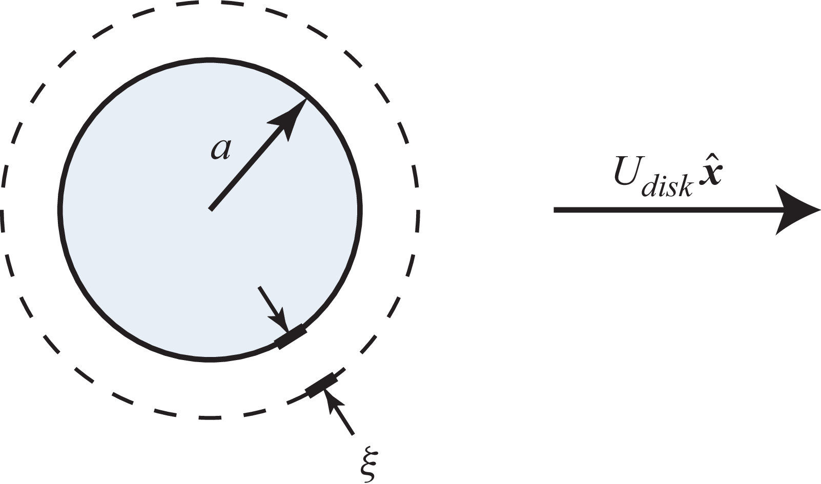
Schematic of a two-dimensional circular disk of radius,
 $a$
, and barrier height,
 $V_0$
, moving at constant velocity,
 $U_{\textit{disk}}$
in the
 $x$
direction, in a superfluid; the Cartesian basis vector,
 $\boldsymbol{\hat {x}}$
, is shown. The ground state is manifest in a reduced fluid density near the disk, whose length scale is the healing length,
 $\xi$
, in (2.19). The flow becomes sonic at the poles of the disk, located at its upper and lower points, at the disk speed,
 $U_{\textit{critical}}$
, when
 $a/\xi \gg 1$
.

The critical body speed for the onset of vortex shedding occurs when the flow first becomes locally sonic at some point on the body, marking the transition to transonic conditions (Rica Reference Rica1993; Huepe & Brachet Reference Huepe and Brachet2000; Rica Reference Rica2001; Huynh et al. Reference Huynh, Hébert, Albert and Larré2024). For rectilinear translation of a two-dimensional circular disk, this occurs at the poles of its cross-section where the fluid speed relative to the disk exceeds the disk’s speed; see figure 1. Consequently, the critical body speed at which vortex shedding and, hence, drag are generated is usually less than the sound speed of the superfluid. The critical body speed for a two-dimensional impenetrable circular disk, whose radius is much larger than the quantum healing length, has been calculated using a Janzen–Rayleigh expansion for compressible potential flow (Rica Reference Rica2001), giving
 \begin{equation} U_{\textit{critical}} = (0.36969\pm 0.00007) c_{\!L}. \end{equation}
This result is supported by studies that numerically solve the GP equation for its stationary states, with the critical speed occurring at their bifurcation point (Huepe & Brachet Reference Huepe and Brachet2000).
Motion of a body in a superfluid can be modelled using a moving external potential (Winiecki, McCann & Adams Reference Winiecki, McCann and Adams1999). This potential provides a barrier within which the fluid is excluded (an impenetrable body) or restricted (a penetrable body), depending on the barrier height relative to the chemical potential of the superfluid. It can therefore describe a solid (impenetrable) body moving through a superfluid and motion of a (penetrable) laser beam through a Bose–Einstein condensate. For example, Desbuquois et al. (Reference Desbuquois, Chomaz, Yefsah, Leonard, Beugnon, Weitenberg and Dalibard2012) examined the superfluidity of a trapped two-dimensional gas of
 $^{87} \text{Rb}$
atoms with a focused laser beam moving at constant velocity; see details in § 6. The drag experienced by an impenetrable circular disk has been studied thoroughly, particularly for disks whose radii exceed the healing length (Frisch et al. Reference Frisch, Pomeau and Rica1992; Winiecki et al. Reference Winiecki, McCann and Adams1999). These studies show that the drag increases monotonically with disk speed, above the critical speed for vortex shedding, with no drag below this critical speed.
Recent theoretical and experimental studies have explored the effect of moving a potential barrier with finite penetrability through a superfluid, focusing in particular on Bose–Einstein condensates (Kwon et al. Reference Kwon, Moon, Seo and Shin2015; Kwak, Jung & Shin Reference Kwak, Jung and Shin2023; Huynh et al. Reference Huynh, Hébert, Albert and Larré2024; Kokubo, Takeuchi & Kasamatsu Reference Kokubo, Takeuchi and Kasamatsu2025). These studies show that the critical speed,
 $U_{\textit{critical}}$
, for the generation of vortices by a moving circular or Gaussian obstacle is minimised when the barrier height matches the chemical potential of the fluid. While the drag experienced by impenetrable bodies is well understood, the drag experienced by a moving penetrable body is yet to be reported and is the focus of this study. That is, the force exerted by a (penetrable) laser spot on a Bose–Einstein condensate is unknown currently. We therefore examine the drag experienced by a two-dimensional potential barrier of circular cross-section – henceforth referred to as the ‘disk’ – moving through a superfluid, as a function of its barrier height. A potential of constant barrier height is chosen to facilitate analytical evaluation while recovering the behaviour of a solid disk in the impenetrable limit. The drag is calculated analytically in the ‘high-speed’ limit, i.e. the disk speed greatly exceeds the fluid sound speed, the results of which are compared with a direct numerical solution (DNS) of the GP equation.
The GP equation along with its equivalent hydrodynamic description, thermodynamic quantities and non-dimensionalisation are summarised in § 2. The problem under investigation is then defined in § 3. Section 4 gives analytical formulas for the drag experienced by impenetrable and highly-penetrable disks, in the classical high-speed limit, with derivation of the latter formula reported in Appendix A. Appendix B reports the corresponding solution for a disk of arbitrary penetrability according to the linear Schrödinger equation, which omits the fluid–particle interaction term in the GP equation. A summary of the numerical method used to directly solve the GP and linear Schrödinger equations is given in § 5, with details reported in Appendix C and a convergence study in Appendix D. Section 6 gives results of the DNS and provides a comparison to the analytical formulas, with auxiliary results in the supplementary material available at https://doi.org/10.1017/jfm.2026.11467. Appendix E discusses computation of the vortex shedding frequency while Appendix F explores the effect of an asymmetric wake. A summary of the findings is given in § 7, which concludes the study.
2. Governing equations
We begin by defining the governing equations used in this study to compute the drag experienced by a disk moving through a superfluid and their non-dimensionalisation.
2.1. The GP equation
The GP equation (Pitaevskii & Stringari Reference Pitaevskii and Stringari2003),
 \begin{equation} i \hbar \frac {\partial \psi (\boldsymbol{r}, t)}{\partial t} = \left [ -\frac {\hbar ^2}{2m} {\nabla} ^2 + V_{\textit{ext}}(\boldsymbol{r}, t) + g |\psi (\boldsymbol{r}, t)|^2 \right ] \psi (\boldsymbol{r}, t), \end{equation}
is a nonlinear Schrödinger equation governing the wavefunction,
 $\psi$
, of a weakly interacting superfluid, such as a Bose–Einstein condensate, where
 $\hbar$
is the reduced Planck constant,
 $\boldsymbol{r}$
is position,
 $t$
is time,
 $m$
is the particle (boson) mass,
 $V_{\textit{ext}}$
is the external potential used to model a moving body,
 $g$
is the interaction strength between particles and
 $i$
is the imaginary unit. The wavefunction,
 $\psi$
, and its gradient,
 $\boldsymbol{\nabla }\psi$
, are continuous throughout the flow domain.
Hydrodynamic equations and thermodynamic quantities arising from (2.1) are summarised in the next section. These highlight the nature of quantum superflows relative to classical potential flows, and define key quantities for this study.
2.2. Hydrodynamic equations and thermodynamic quantities
Equation (2.1) can be transformed into a system of equations resembling those of classical fluid mechanics using the polar form (Madelung Reference Madelung1927),
 \begin{equation} \psi (\boldsymbol{r}, t) \equiv n^{\frac {1}{2}} \exp {(i S)}, \end{equation}
where
 $n\, (\equiv \! |\psi |^2)$
is the number density of superfluid particles and
 $S$
is the phase. The corresponding mass density of the fluid is
 \begin{equation} \rho \equiv m n = m | \psi |^2. \end{equation}
The momentum current density is (Pitaevskii & Stringari Reference Pitaevskii and Stringari2003)
 \begin{equation} \boldsymbol{J} \equiv \frac {\hbar }{2 i} \left (\psi ^* \boldsymbol{\nabla }\psi - \psi \boldsymbol{\nabla }\psi ^* \right )\!, \end{equation}
where the superscript
 $^*$
denotes the complex conjugate. Substituting (2.2) into (2.4) and using (2.3), gives the required fluid velocity,
 \begin{equation} \boldsymbol{u} \equiv \frac {\boldsymbol{J}}{\rho } = \frac {\hbar }{m} \boldsymbol{\nabla }\!S, \end{equation}
showing that the GP equation generates a potential flow. Equations (2.2) and (2.5) then establish that the circulation around any vortex is quantised in integer multiples of
 $2 \pi\! \hbar / m$
; this contrasts with a classical fluid, for which no such constraint exists.
The continuity equation follows from multiplying (2.1) by
 $\psi ^*$
, then multiplying the resulting expression by its complex conjugate and taking the difference between these two expressions, giving
 \begin{equation} \frac {\partial \rho }{\partial t} + \boldsymbol{\nabla }\boldsymbol{\cdot }\boldsymbol{J} = 0, \end{equation}
which together with (2.5) is identical to the classical continuity equation.
The momentum equation is derived by differentiating (2.4) with respect to time, and making use of (2.1), to give
 \begin{equation} \frac {\partial \boldsymbol{J}}{\partial t} + \boldsymbol{\nabla }\boldsymbol{\cdot }\boldsymbol{\varPi } + \rho \boldsymbol{\nabla }\left ( \frac {V_{\textit{ext}}}{m} \right ) = \boldsymbol{0}, \end{equation}
where
 $\boldsymbol{\varPi }$
is the momentum flux density,
 \begin{equation} \boldsymbol{\varPi } = \frac {\hbar ^2}{4 m} \left ( \boldsymbol{\nabla }\psi ^* \boldsymbol{\nabla }\psi - \psi ^* \boldsymbol{\nabla }\boldsymbol{\nabla }\psi + \text{C.C.} \right ) + \frac {g}{2} |\psi |^4 \boldsymbol{I}, \end{equation}
with
 $\boldsymbol{I}$
being the identity tensor and ‘C.C.’ denoting the complex conjugate of the terms that precede it. Adding
 $\boldsymbol{\nabla }\boldsymbol{\cdot }(\rho \boldsymbol{u} \boldsymbol{u})$
to both sides of (2.7), and making use of (2.2) and (2.5), gives the Cauchy equation of motion with the superfluid stress tensor,
 \begin{equation} \boldsymbol{T} \equiv \rho \, \boldsymbol{u} \boldsymbol{u} - \boldsymbol{\varPi } = \left (\frac {\hbar }{2 m}\right )^2 \rho \, \boldsymbol{\nabla }\boldsymbol{\nabla }\ln \rho - \frac {g}{2} \left (\frac {\rho }{m}\right )^2 \boldsymbol{I}, \end{equation}
which is not isotropic and differs from a classical Euler (ideal) fluid, i.e. the superfluid is not an Euler fluid despite generating a potential flow.
Substituting (2.9) into the Cauchy equation of motion gives the superfluid Bernoulli equation,
 \begin{equation} \hbar \frac {\partial S}{\partial t} + \frac {1}{2} m | \boldsymbol{u} |^2 + \frac {g \rho }{m} - \left (\frac {\hbar ^2}{2 m}\right ) \rho ^{-\frac {1}{2}} {\nabla} ^2 \rho ^{\frac {1}{2}} + V_{\textit{ext}} = f(t) , \end{equation}
which applies throughout the flow domain (because a potential flow exists), where
 $f$
is an arbitrary function of time. A Bernoulli equation is expected because (2.1) conserves energy (Pitaevskii & Stringari Reference Pitaevskii and Stringari2003). Equation (2.10) differs from the Bernoulli equation for a classical potential flow due to the appearance of the quantum pressure term (fourth term on the left-hand side) and Planck’s constant. That is, the superfluid is not an ideal Euler fluid unless the quantum pressure term is zero or can be neglected.
The mechanical pressure,
 $p_{\textit{mech}} \equiv -1/3 \, \text{tr} \, \boldsymbol{T}$
, follows from (2.9),
 \begin{equation} p_{\textit{mech}} = - \frac {1}{3} \left (\frac {\hbar }{2 m}\right )^2 \rho \,{\nabla} ^2 \ln \rho + \frac {g}{2} \left (\frac {\rho }{m}\right )^2\! , \end{equation}
where the first term is due to the quantum stress arising from field gradients and the second term originates from the (nonlinear) particle interaction energy in the GP mean-field Hamiltonian (Pitaevskii & Stringari Reference Pitaevskii and Stringari2003); see the numerator in (2.16). In the absence of spatial gradients, the mechanical pressure reduces to an effective interaction-induced pressure,
 \begin{equation} p = \frac {g}{2} \left (\frac {\rho }{m}\right )^2\! , \end{equation}
which defines a barotropic pressure–density relation for the fluid. Although this relation is not thermodynamic in origin, it plays the role of an effective equation of state in the hydrodynamic formulation of the GP equation. The corresponding barotropic index of
 $\gamma = 2$
exceeds that of any classical compressible fluid.
The sound (Landau) speed of the superfluid follows from (2.12),
 \begin{equation} c_{\!L} \equiv \left . \sqrt {\frac {\partial p}{\partial \rho }} \, \right |_{\, \rho \, = \, \rho _\infty } = \sqrt {\frac {gn_\infty }{m}}, \end{equation}
where
 $n_\infty = \rho _\infty / m$
is the bulk number density with
 $\rho _\infty$
being the bulk mass density.
The chemical potential,
 $\mu$
, of the system obeying the GP equation (2.1) can be computed from the stationary state,
 \begin{equation} \psi (\boldsymbol{r}, t) = \phi (\boldsymbol{r}) \exp \!\left (-\frac {i \mu t}{\hbar }\right )\!, \end{equation}
which upon substitution into (2.1) yields
 \begin{equation} \mu \phi = \left [ -\frac {\hbar ^2}{2m} {\nabla} ^2 + V_{\textit{ext}} + g |\phi |^2 \right ] \phi . \end{equation}
Multiplying (2.15) by
 $\phi ^*$
and integrating over the flow domain,
 $V$
, gives the required result,
 \begin{equation} \mu = \frac {\int _V \dfrac {\hbar ^2}{2m} | \boldsymbol{\nabla }\psi |^2 + V_{\textit{ext}} |\psi |^2 + g |\psi |^4 \, {\rm d}V }{\int _V |\psi |^2 \, {\rm d}V}, \end{equation}
where (2.14) has been used and the absence of spatial gradients in
 $\psi$
at the domain boundary is imposed. The numerator is the expectation value of the GP mean-field Hamiltonian, while the denominator is the total number of particles. Owing to the (nonlinear) interaction term being proportional to
 $g$
in (2.16),
 $\mu$
differs from the total energy per particle and instead corresponds to the chemical potential, i.e. the energy required to add one particle.
The hydrodynamic equations and thermodynamic quantities summarised in this section show that while quantum superflows obeying the GP equation exhibit some features of classical flows, they represent a distinct class of flow.
2.3. Dimensionless governing equations
An appropriate non-dimensionalisation of the wavefunction follows from (2.2),
 \begin{equation} \psi = \sqrt {n_\infty } \, \bar {\psi }, \end{equation}
where the overbar denotes a dimensionless variable. Substituting (2.17) into (2.1), balancing all terms and making use of (2.16), gives the dimensionless variables,
 \begin{equation} t = \frac {\hbar }{gn_\infty } \bar {t}, \quad \boldsymbol{r} = \frac {\hbar }{\sqrt {m gn_\infty }} \bar {\boldsymbol{r}}, \quad V_{\textit{ext}} = gn_\infty \bar {V}_{\textit{ext}}, \quad \mu = gn_\infty \bar {\mu }, \end{equation}
from which the velocity scale is the ratio of the length and time scales, and is identical to the sound speed in (2.13). The length scale in (2.18) is termed the ‘healing length’ and denoted as
 \begin{equation} \xi \equiv \frac {\hbar }{\sqrt {m gn_\infty }} . \end{equation}
Consequently, the dimensionless GP equation is
 \begin{equation} i \frac {\partial \psi }{\partial t} = \left [ -\frac {1}{2}{\nabla} ^2 + V_{\textit{ext}} + |\psi |^2 \right ] \psi , \end{equation}
where we henceforth omit the overbar notation while noting that all variables are dimensionless, unless specified otherwise. The corresponding dimensionless Bernoulli equation is
 \begin{equation} \frac {\partial S}{\partial t} + \frac {1}{2} | \boldsymbol{u} |^2 + n - \frac {1}{2 n^{\frac {1}{2}}} {\nabla} ^2 n^{\frac {1}{2}} + V_{\textit{ext}} = f(t) , \end{equation}
where the dimensionless number density,
 $n$
, is scaled by its bulk value, and the dimensionless velocity is
 \begin{equation} \boldsymbol{u} = \boldsymbol{\nabla }\!S, \end{equation}
with the phase,
 $S$
, being implicitly dimensionless.
3. Problem statement
The drag experienced by a disk – i.e. a circular potential barrier of constant height,
 $V_0$
, as defined above – moving in an unbounded quiescent superfluid is sought. The disk is initially at rest with the system in its ground state. At time,
 $t=0$
, the disk moves impulsively at constant velocity,
 $U_{\textit{disk}}$
in the
 $x$
direction; see figure 1. The fluid’s initial ground state and subsequent dynamics obey the GP equation (2.20). The instantaneous drag and its steady-state value (after all start-up transients have decayed) are sought as a function of the disk’s barrier height,
 $V_0$
, and its speed,
 $U_{\textit{disk}}$
. The problem depends on three dimensionless variables of the disk, specifically its
-
(i) radius,
 $R$
, which is scaled by the healing length in (2.19);
-
(ii) speed,
$U_{\textit{disk}}$
, which is scaled by the sound speed in (2.13), and -
(iii) barrier height,
$V_0$
, which is scaled by the bulk chemical potential of the fluid in (2.18).


This study primarily focuses on the near-classical regime where quantum wave effects are small, which is now defined.
3.1. Classical limit
The disturbance flow generated by a disk moving at constant speed,
 $U_{\textit{disk}}$
, through a quiescent unbounded fluid is equivalent to that produced by a uniform flow of speed,
 $U_{\textit{disk}}$
, impinging on a stationary disk. A uniform superflow corresponds to a plane wave of the wavefunction,
 $\psi$
. It follows that the dimensionless wavenumber associated with the disturbance flow generated by the disk is
 $k a$
; where in dimensional variables
 $k \equiv m U_{\textit{disk}} / \hbar$
is the flow-induced wavenumber and
 $a$
is the disk radius. Using the scalings in § 2.3, this dimensionless wavenumber becomes
 \begin{equation} k a = U_{\textit{disk}} R, \end{equation}
where
 $U_{\textit{disk}}$
and
 $R$
are the dimensionless disk speed and radius, respectively. The classical (hydrodynamic or geometrical optics) limit, where the quantum pressure term in (2.10) is subdominant, corresponds to
 \begin{equation} U_{\textit{disk}} R \gg 1. \end{equation}
When (3.2) holds, the flow admits a classical hydrodynamic description with quantum pressure effects suppressed but mean-field particle interactions retained.
4. High-speed limit
Analytical formulas for the drag in the high-speed limit, i.e.
 $U_{\textit{disk}} \gg 1$
, are reported in this section. Particle interactions in (2.20) can be neglected to calculate the drag in this limit (Winiecki Reference Winiecki2001), with (2.20) becoming the linear Schrödinger equation,
 \begin{equation} i \frac {\partial \psi }{\partial t} = \left [ -\frac {1}{2} {\nabla} ^2 + V_{\textit{ext}} \right ] \psi , \end{equation}
which facilitates an analytical solution. This problem is solved in the frame of the disk, and thus,
 \begin{equation} V_{\textit{ext}}(r) = \left \{\! \begin{array}{ll}V_0, & r \leqslant R, \\0, & r \gt R,\end{array}\right . \end{equation}
where
 $V_0$
is the barrier height and
 $r \equiv |\boldsymbol{r}|$
is the radial coordinate whose origin is the disk centre. A uniform flow of velocity,
 $U_{\textit{disk}}$
in the negative
 $x$
direction, is therefore imposed far from the disk, with a chemical potential (for
 $U_{\textit{disk}} \gg 1$
) of
 \begin{equation} \mu = \frac {1}{2} U_{\textit{disk}}^2. \end{equation}
The resulting steady flow is given by the stationary solution,
 \begin{equation} \psi (\boldsymbol{r}) = \phi (\boldsymbol{r}) \exp \!\left (-i \mu t\right )\!, \end{equation}
from which (4.1) becomes
 \begin{equation} \left [ -\frac {1}{2} {\nabla} ^2 + V_{\textit{ext}}(\boldsymbol{r}) - \mu \right ] \! \phi (\boldsymbol{r}) = 0. \end{equation}
It is evident from (4.2) and (4.5) that particle interactions in (2.20) cannot be formally neglected when
 $V_0 \approx \mu$
, with the particle interaction term in (2.20) becoming dominant even at high disk speed. Therefore, the drag derived from (4.5) is a solution of (2.20) at high disk speed provided
 $V_0 \ll \mu$
or
 $V_0 \gg \mu$
; these limits only are considered in this section.
A uniform superflow of velocity,
 $U_{\textit{disk}}$
in the negative
 $x$
direction, corresponds to a plane wave of the wavefunction,
 $\phi = \exp (-i U_{\textit{disk}}\, r \cos \theta )$
, in polar coordinates,
 $(r, \theta )$
, centred on the disk. The angle,
 $\theta$
, is measured anticlockwise relative to the
 $x$
axis; see figure 1. The corresponding far-field wavefunction,
 $\phi _{\textit{sc}}$
, scattered by the disk is then (Griffiths & Schroeter Reference Griffiths and Schroeter2018)
 \begin{equation} \phi _{\textit{sc}}(r,\theta )\sim \frac {1}{\sqrt {r}}\,e^{i\left (U_{\textit{disk}} \, r+\frac {\pi }{4}\right )}\,f(\theta ), \quad r\to \infty , \end{equation}
with
 $f(\theta )$
being the scattering amplitude, which is to be determined. The drag per unit length (henceforth referred to simply as the drag) experienced by the disk can be expressed as
 \begin{equation} F_{\textit{drag}} = \sigma U_{\textit{disk}}^2 , \end{equation}
where
 $\sigma$
is the two-dimensional momentum transfer cross-section per unit length given by
 \begin{equation} \sigma = \int _0^{2 \pi } (1-\cos \theta ) | f(\theta ) |^2 \, {\rm d} \theta . \end{equation}
The drag experienced by a disk moving at high speed in a superfluid is therefore determined by solving the linear Schrödinger equation (4.1), for the scattering of a plane wave by a circular barrier (Griffiths & Schroeter Reference Griffiths and Schroeter2018).
An impenetrable disk corresponds to
 $V_0 \gg \mu$
, where
 $\mu$
is defined in (4.3), while the opposite limit of
 $\mu \gg V_0$
yields a highly penetrable disk. The former case pertains to situations where the particle kinetic energy is far smaller than the barrier height, with the latter being the opposite limit.
4.1. Impenetrable disk
The drag experienced by an impenetrable disk moving at high speed, in the classical limit, is
 \begin{equation} F_{\textit{drag}} = \frac {8}{3} R U_{\textit{disk}}^2, \quad 1 \ll U_{\textit{disk}} \ll \sqrt {2 V_0}, \end{equation}
which was derived in Winiecki (Reference Winiecki2001) by solving (4.5) using an eigenfunction expansion, the general solution of which was expanded for large
 $U_{\textit{disk}} R$
. Equation (4.9) was found to agree with DNS at high disk speeds,
 $U_{\textit{disk}} \gg 1$
, for disk radii,
 $R \gt 1$
(Winiecki et al. Reference Winiecki, McCann and Adams1999).
4.2. Highly penetrable disk
The corresponding drag experienced by a highly penetrable disk in the classical limit is
 \begin{equation} F_{\textit{drag}} = 2 R \left ( \frac {V_0}{U_{\textit{disk}}} \right )^2 \, \big [ 5 \log 2 -2 + \gamma + \log \! \left ( U_{\textit{disk}} R \right ) \! \big ] , \quad 1 \ll \sqrt {2 V_0} \ll U_{\textit{disk}}, \end{equation}
where
 $\gamma = 0.5772\ldots$
is Euler’s constant, the derivation of which is reported in Appendix A.
The asymptotic formulas in (4.9) and (4.10) are compared with the drag arising from the exact analytical solution to (4.5) for a circular disk of arbitrary scaled strength,
 $2 V_0 / U_{\textit{disk}}^2$
, in Appendix D.1.
4.3. Summary
The formulas in (4.9) and (4.10) establish that the classical drag at high speed increases quadratically with
 $U_{\textit{disk}}$
for an impenetrable disk, while decreasing with a logarithmically modulated inverse-quadratic dependence on
 $U_{\textit{disk}}$
when the disk is highly penetrable. This suggests that the drag exhibits a unimodal dependence on disk speed,
 $U_{\textit{disk}}$
, with a single maximum drag occurring at intermediate speeds, i.e.
 $U_{\textit{disk}} \sim \sqrt {2 V_0}$
, and monotonic behaviour at other speeds. Substituting this expression into (4.9) and (4.10) indicates that, in the high-speed, classical limit, the maximum drag experienced by a penetrable disk scales as
 \begin{equation} F_{\textit{drag}}^{\textit{max}} \sim R V_0, \qquad U_{\textit{disk}} \gg 1. \end{equation}
In the next section, (4.9)–(4.11) are compared with DNS of the GP equation (2.20), which includes the effect of particle interactions and applies to all disk speeds.
5. Numerical method
A graphics processing unit (GPU) accelerated split-time spectral method is used to directly solve (2.20) and (4.1), the details of which are provided in Appendix C. A square computational domain with identical spatial discretisation in the
 $x$
and
 $y$
directions is used in all simulations, i.e.
 $L \equiv L_x = L_y$
and
 $N \equiv N_x = N_y$
, respectively. Because the drag experienced by a disk moving in an unbounded domain is sought, the computational domain is chosen to be large relative to the disk radius, i.e.
 $L \gg R$
, to minimise boundary effects. The number of grid points is set to
 \begin{equation} N = 2^\alpha + 1, \end{equation}
where
 $\alpha$
is a positive integer, enabling use of the fast discrete cosine transform. The domain size is then chosen to be
 \begin{equation} L = 2^{- \beta } (N-1)= 2^{\alpha - \beta }, \end{equation}
where
 $\beta$
is a positive integer, ensuring the spatial grid discretisation in the
 $x$
and
 $y$
directions,
 \begin{equation} \Delta x = \Delta y = \frac {L}{N-1} = 2^{- \beta }, \end{equation}
is less than the healing length (which is scaled to unity). The spatial discretisation,
 $\Delta x$
, is refined to capture the smallest length scale of the flow, which includes the minimum of (i) the healing length, i.e. unity; (ii) the disk radius,
 $R$
; and (iii) the quantum wavelength,
 $2 \pi / U_{\textit{disk}}$
(see § 4). The corresponding time step is set to
 \begin{equation} \Delta t = \left (\frac {\Delta x}{\pi }\right )^2 = \pi ^{-2} 2^{-2\beta } . \end{equation}
These equations show that
 $\beta$
controls the grid discretisation and time step, while the difference,
 $\alpha - \beta$
, sets the domain size.
The results presented in this study are based on approximately 3000 individual numerical simulations, with a maximum number of grid points of
 $(N\times N)= (4097\times 4097)$
. Convergence studies of this numerical method are reported in Appendix D, where the present numerical method is validated using the exact analytical solution to (4.1) and benchmarked against literature data for (2.20). This shows that the use of an insufficiently fine spatial discretisation can produce spurious oscillations in the force, which have previously been interpreted as physically real.
6. Results and discussion
The flow and drag generated by a circular disk started impulsively from rest and moving at constant rectilinear speed,
 $U_{\textit{disk}}$
, are now explored. This is achieved by solving the GP equation (2.20), using the DNS method described in § 5 and Appendix C. Results are reported for disks of radii
 $R = 1$
,
 $3$
and
 $5$
, with the classical limit corresponding to cases where
 $U_{\textit{disk}} R \gg 1$
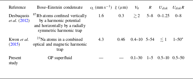
(see § 3.1). A comparison of experimental parameters reported in the literature with those used in this study is given in table 1.
Comparison of the experimental Bose–Einstein condensate parameters reported in the literature and the dimensionless parameters used in the present study. Note that experimental studies use a moving obstacle in the form of a Gaussian laser beam while the present study employs a disk with a step barrier height; see § 1 and (4.2). For these Gaussian beams,
 $V_0$
refers to the Gaussian height scaled by the chemical potential while
 $R$
is the Gaussian width scaled by the healing length.
 $^\ast$
Assuming the maximum obstacle speed is twice its critical speed; maximum speed not reported.

6.1. Impenetrable disk
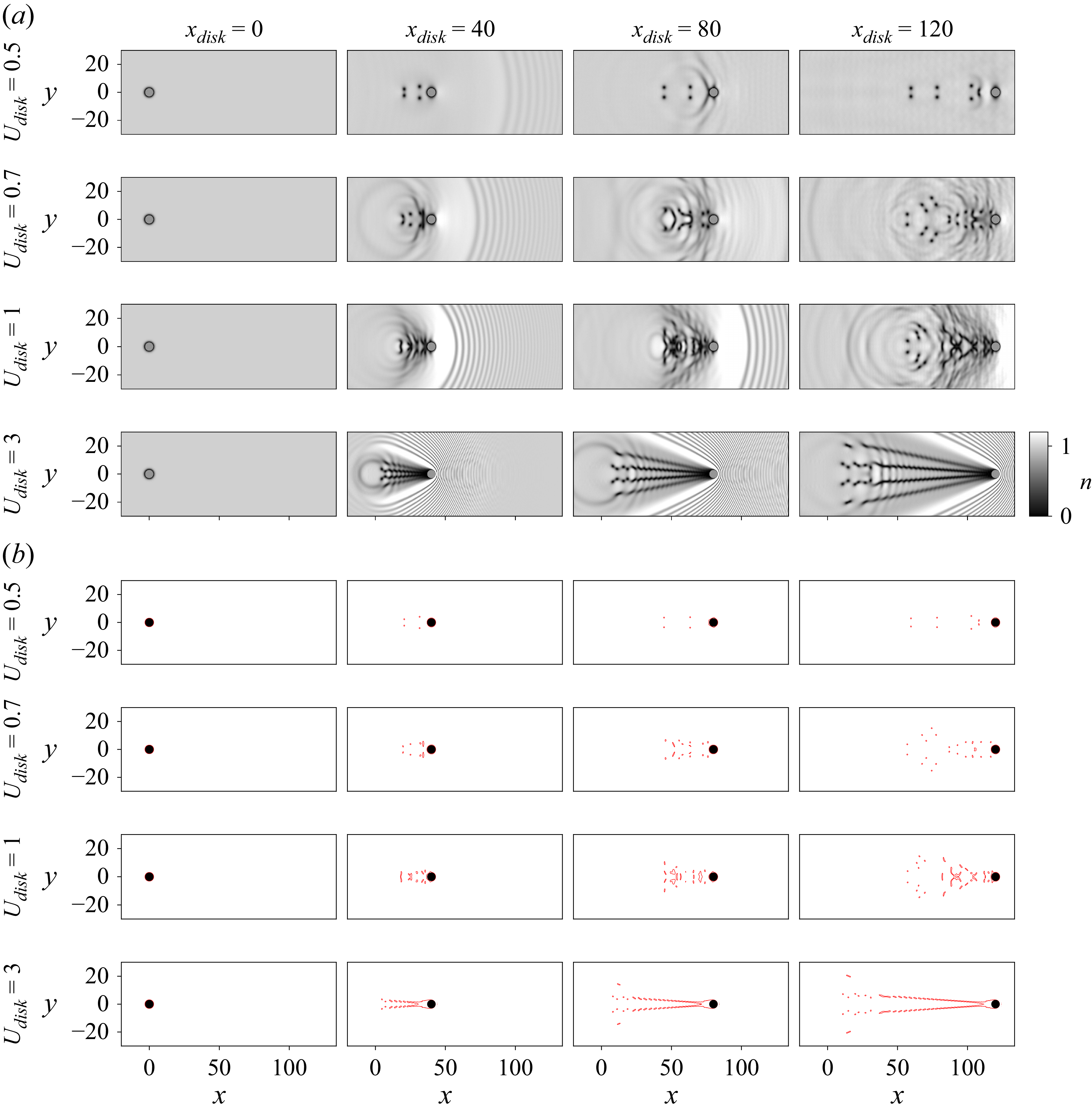
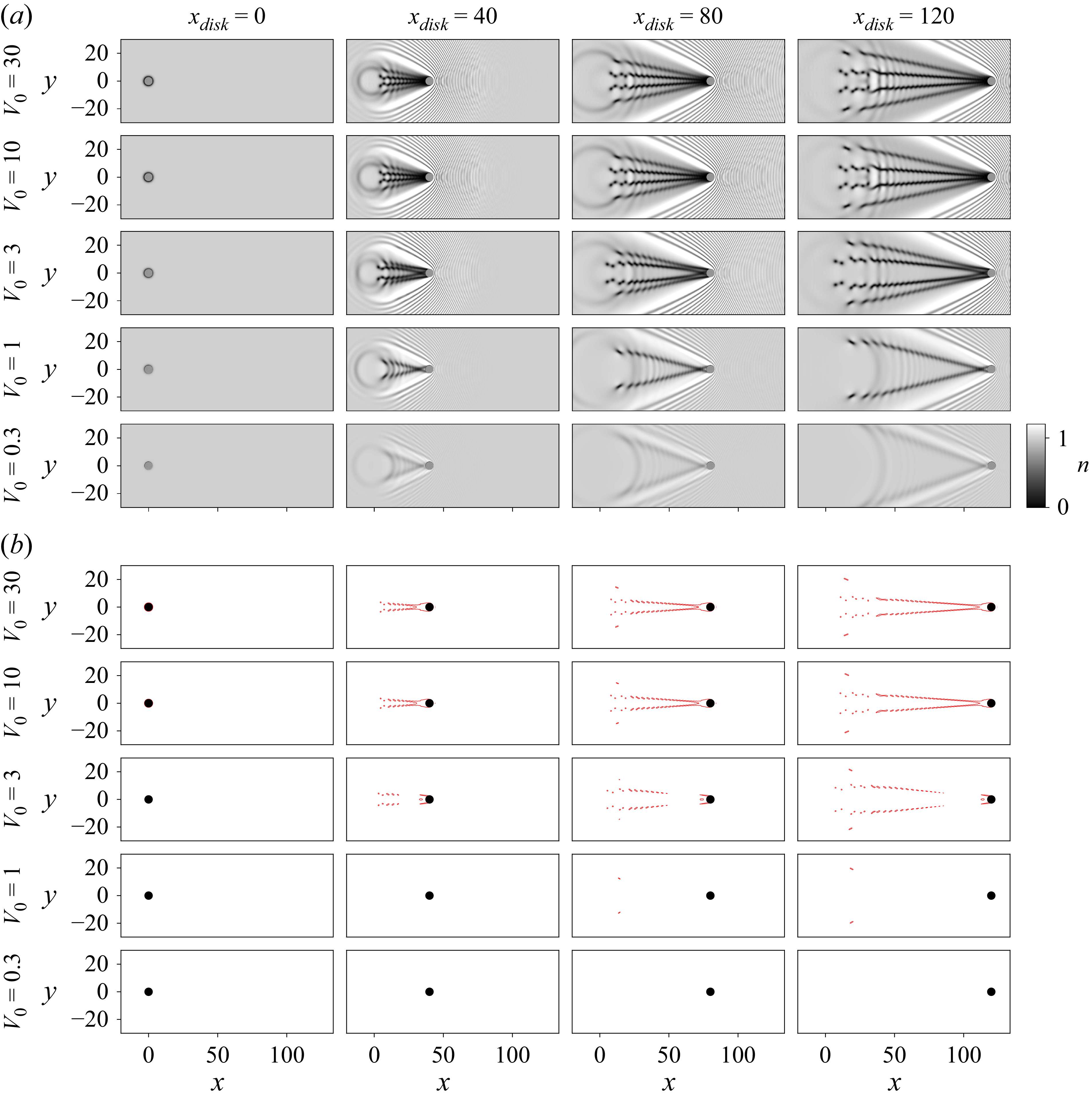
Impenetrable disk. Evolution of superfluid density for a disk of radius,
 $R = 3$
(a grey filled circles; b black filled circles), started impulsively from rest at
 $x = x_{\textit{disk}} = 0$
that subsequently moves with a constant velocity of
 $U_{\textit{disk}}$
in the
 $x$
direction. (a) Number density distribution. (b) Level sets of small number density,
 $n = 0.1$
, highlight the vortex positions and dark solitons. Results are shown for disk speeds,
 $U_{\textit{disk}} = 0.5, 0.7, 1, 3$
. Computational parameters:
 $N=2049$
,
 $L = 256$
and
 $\Delta x = 1/8$
(
 $\alpha = 11$
and
 $\beta = 3$
),
 $V_0=30$
with
 $\Delta t$
given by (5.4).

We first examine the widely studied flow generated by an impenetrable disk (
 $U_{\textit{disk}}\ll \sqrt {2 V_0}$
; see § 4) that moves impulsively at constant rectilinear velocity in a quiescent superfluid (Frisch et al. Reference Frisch, Pomeau and Rica1992; Winiecki et al. Reference Winiecki, McCann and Adams1999; Huepe & Brachet Reference Huepe and Brachet2000; El, Gammal & Kamchatnov Reference El, Gammal and Kamchatnov2006). This sets a baseline for exploring the effects of finite disk penetrability, which is the focus of the present study.
6.1.1. Flow structures
Figure 2 reports the evolution of the number density distribution,
 $n$
, following impulsive motion of a disk of radius,
 $R = 3$
, from rest. Results are shown for various disk speeds,
 $U_{\textit{disk}}=0.5$
,
 $0.7$
,
 $1$
and 3, spanning subsonic to supersonic flows. Disk speeds below the dimensionless critical speed,
 $U_{\textit{critical}} \approx 0.37$
in (1.1), do not generate vortices (data not shown). The critical speed is known to increase with decreasing disk radius,
 $R$
, which aligns with the results for
 $R = 1$
and
 $U_{\textit{disk}} = 0.5$
in figure S1 of the supplementary material, where vortices are not generated. Figure 2(b) shows level sets of small number density (
 $n=0.1$
) to highlight the vortex positions, which occur where the number density is zero. Bow waves are generated by the impulsive disk start up in all cases. These bow waves move away from the disk when it moves at subsonic speeds, i.e.
 $U_{\textit{disk}} \lt 1$
. At the chosen supersonic disk speed,
 $U_{\textit{disk}} = 3\, (\gt \!\! 1)$
, a Mach cone forms. Discrete vortices generate their own wave motion as they are shed and interact. This wave motion is distinct from the bow wave discussed above.
Discrete quantum vortices nucleate at or near the poles of the disk at subsonic and transonic speeds,
 $U_{\textit{disk}} \leqslant 1$
; see figure 2. These are weakly advected by the disturbance flow generated by the moving disk. The vortices are confirmed to have a dimensionless circulation of
 $\pm 2 \pi$
(data not shown); see § 2.2. The structure of the wake changes dramatically as the disk speed,
 $U_{\textit{disk}}$
, is varied. Widely spaced vortices occur at subsonic disk speeds that compactify as the disk speed becomes supersonic. When
 $U_{\textit{disk}} \leqslant 1$
, vortices shed and move in a random aperiodic fashion. This is highlighted by the level set plots in figure 2(b). A significant difference is observed at the supersonic speed of
 $U_{\textit{disk}}=3$
, with a steady low-density region forming immediately behind the disk that connects to oblique dark solitons. These solitons destablise as they interact with the outgoing cylindrical wave generated by the impulsively started disk, forming vortex dipoles, i.e. localised pairs of vortices with circulations of opposite sign. The number density plots in figure 2(a) show a set of two oblique dark solitons, emanating at different angles. Comparison with the level set plots in figure 2(b) shows that the number density of the outer oblique solitons is larger than those of the inner solitons.
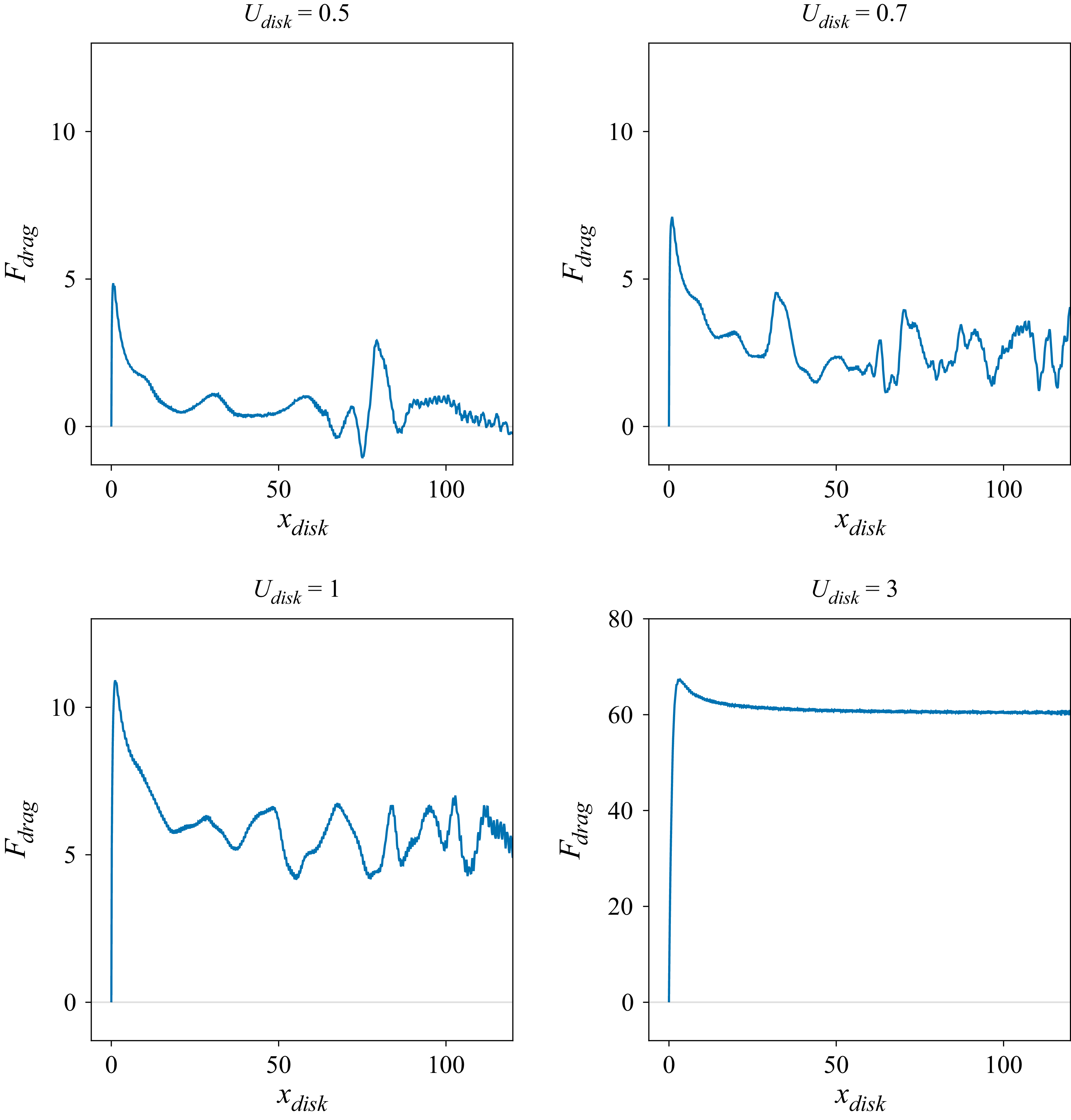
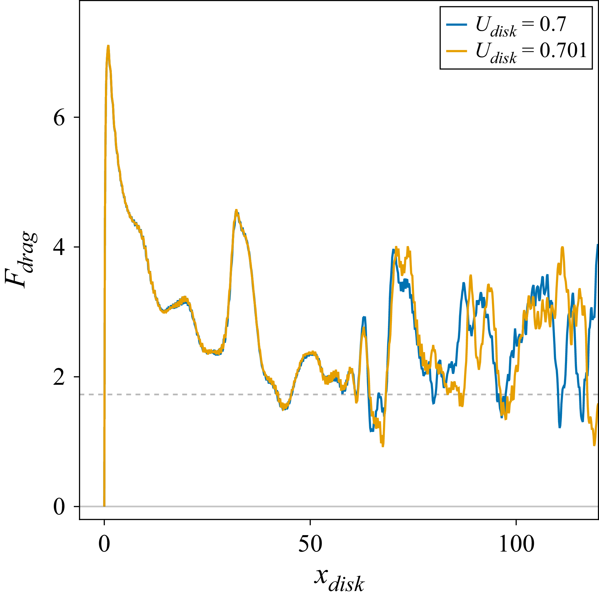
Impenetrable disk. Instantaneous drag as a function of the disk speed,
 $U_{\textit{disk}}$
, for
 $R=3$
; horizontal axis is the disk position. Identical axes scales are used for
 $U_{\textit{disk}} = 0.5, 0.7$
and
 $1$
; a different vertical scale is used for
 $U_{\textit{disk}} = 3$
. Zero drag (horizontal grey line) for reference only. Computational parameters:
 $N=4097$
,
 $L = 256$
and
 $\Delta x = 1/16$
(
 $\alpha = 12$
and
 $\beta = 4$
),
 $V_0=30$
with
 $\Delta t$
given by (5.4).

Impenetrable disk. Evolution of the instantaneous drag,
 $F_{\textit{drag}}$
, showing a sensitive dependence on disk speed,
 $U_{\textit{disk}}$
, and hence, chaotic dynamics. Steady-state time-averaged drag,
 $\langle F_{\textit{drag}}\rangle$
, for both disk speeds are given by the horizontal dashed lines and are visually indistinguishable. Computational parameters as for figure 3.

Complementary results for disk radii of
 $R=1$
and
 $5$
are reported in figures S1 and S2 of the supplementary material, respectively, showing that the number of oblique dark solitons increases linearly with
 $R$
. The healing length (normalised to unity) sets a natural quantum length scale for the superflow, determining both the characteristic size of density variations near boundaries and the core size of vortices; other excitations, such as acoustic waves described by the Bogoliubov dispersion relation, can involve length scales much larger than the healing length. Thus, increasing the disk radius relative to the healing length is expected to increase the number of excitations/vortices shed and decrease their relative spacing with respect to the disk radius, as observed.
6.1.2. Time dependence of the instantaneous drag
Figure 3 gives time series of the instantaneous drag,
 $F_{\textit{drag}}$
, for the flows in figure 2. These results show that
 $F_{\textit{drag}}$
is aperiodic at subsonic-to-transonic disk speeds, i.e.
 $U_{\textit{disk}} = 0.5$
,
 $0.7$
and
 $1$
. The drag,
 $F_{\textit{drag}}$
, is also chaotic with its time series exhibiting a sensitive dependence on the chosen disk speed,
 $U_{\textit{disk}}$
. This is demonstrated in figure 4 by varying the disk speed slightly, from
 $U_{\textit{disk}} = 0.7$
to
 $U_{\textit{disk}} = 0.701$
. Drag evolution for these two disk speeds overlap at smaller disk positions (i.e. time), but diverge abruptly in finite time. Even so, the steady-state time-averaged drag,
 $\langle F_{\textit{drag}} \rangle$
, is insensitive to this small change in disk speed. The magnitudes of these aperiodic/chaotic drag fluctuations, relative to the steady-state time-averaged drag, decrease as the disk speed increases and dramatically fall off for
 $U_{\textit{disk}} \gt 1$
. Results for
 $U_{\textit{disk}} = 3$
display a time-independent steady-state drag, i.e. the drag is independent of time in the second half of the simulation. This is consistent with the change in wake morphology discussed in § 6.1.1, where a steady low-density region emerges behind the disk; see figure 2. Small-amplitude high-frequency oscillations in figures 3 and 4, particularly at longer times, are an unavoidable numerical artefact. They are controlled by the number of grid points and decrease with grid size,
 $\Delta x$
; see Appendix D.2.
Evolution of superfluid density for a disk of radius,
 $R = 3$
(a grey filled circles; b black filled circles), moving with speed,
 $U_{\textit{disk}} = 3$
, started impulsively from rest at
 $x = x_{\textit{disk}} = 0$
. Results are shown as a function of the disk barrier height,
 $V_0$
. (a) Number density distribution. (b) Level sets of small number density,
 $n = 0.1$
, highlight the vortex positions and dark solitons. Computational parameters are as for figure 2.

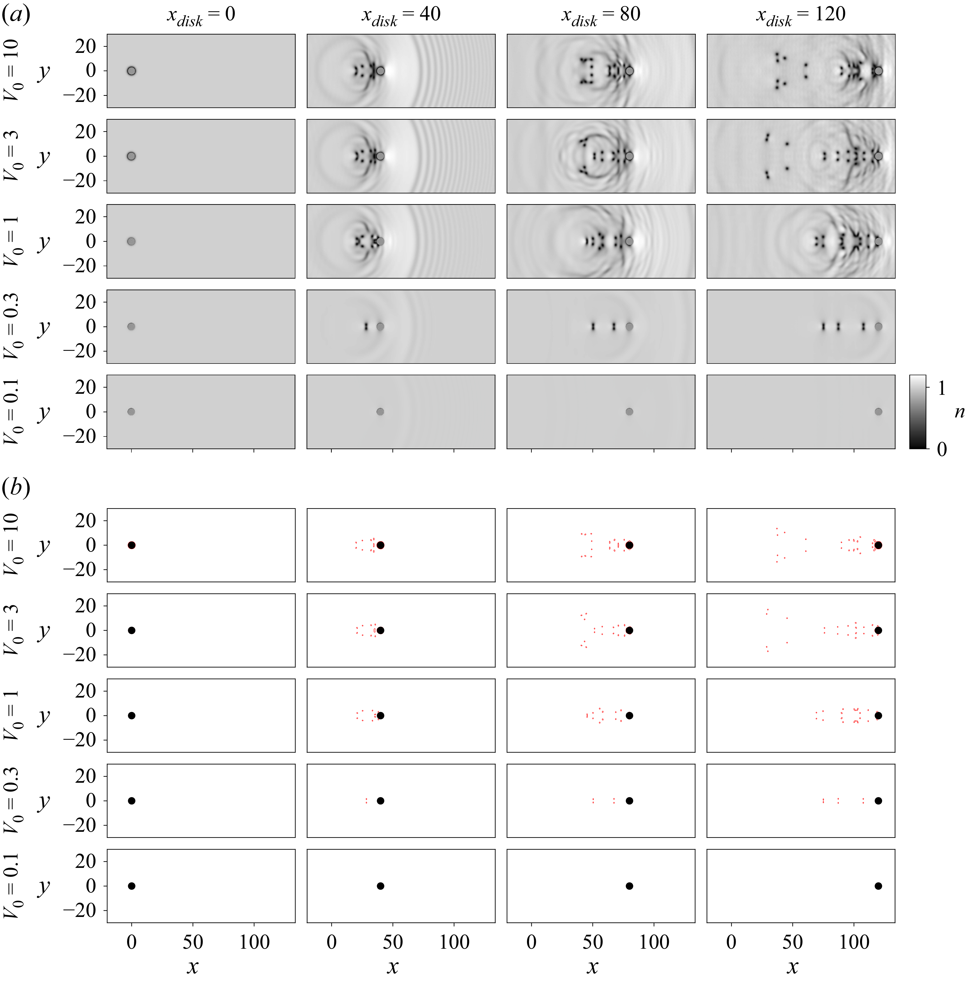
As for figure 5, but with
 $U_{\textit{disk}} = 0.7$
.

These results show that vortex shedding may not be manifest in the drag evolution, which has been used in some previous studies to infer the vortex shedding frequency; see Appendix D.2. Instead, the instantaneous drag is steady at high disk speed for which the vortex shedding frequency can be determined directly from the flow field; see Appendices C.4 and E. Supplementary movies 1–4 available at https://doi.org/10.1017/jfm.2026.11467 elucidate the relationship between the flow features generated by the moving disk and the instantaneous drag time series for all cases shown in figure 2.
6.2. Penetrable disk
We turn our attention to the effect of finite disk penetrability on the drag, which constitutes the primary focus of this study. The influence of varying the barrier height,
 $V_0$
, on the flow field is first examined and compared with the results for an impenetrable disk presented in § 6.1.
6.2.1. Flow structures
Figure 5 gives results for the flow produced by the moving disk, as the barrier height is systematically reduced from its value of
 $V_0 = 30$
in figure 2 to
 $V_0 = 0.3$
, for a fixed (supersonic) disk speed of
 $U_{\textit{disk}} = 3$
. Reducing
 $V_0$
enhances disk penetrability by the fluid.
The analytical theory in § 4 predicts that the disk will be significantly penetrable when
 $V_0 \lesssim (1/2) U_{\textit{disk}}^2$
, i.e.
 $V_0 \lesssim 4.5$
for
 $U_{\textit{disk}} = 3$
. This aligns with the DNS reported in figure 5(b) where a change in the level set plots is observed for a barrier height of
 $V_0 = 3$
, relative to the higher values of
 $V_0 = 10$
and 30 (for which the disk is impenetrable and the wake is insensitive to
 $V_0$
). Decreasing the barrier height to
 $V_0=1$
, leads to a morphological change in the wake with the inner oblique dark solitons vanishing; see number density plot in figure 5(a). Moreover, the
 $n = 0.1$
level sets in figure 5(b) vanish for
 $V_0=1$
, except at the largest disk position,
 $x_{\textit{disk}} = 120$
. This shows that decreasing the disk barrier height not only reduces the number density disturbance, as may be expected, but also affects the wake structure. A further reduction to
 $V_0=0.3$
increases the angle subtended by the oblique dark solitons, which now exhibit a small density perturbation relative to the bulk fluid.
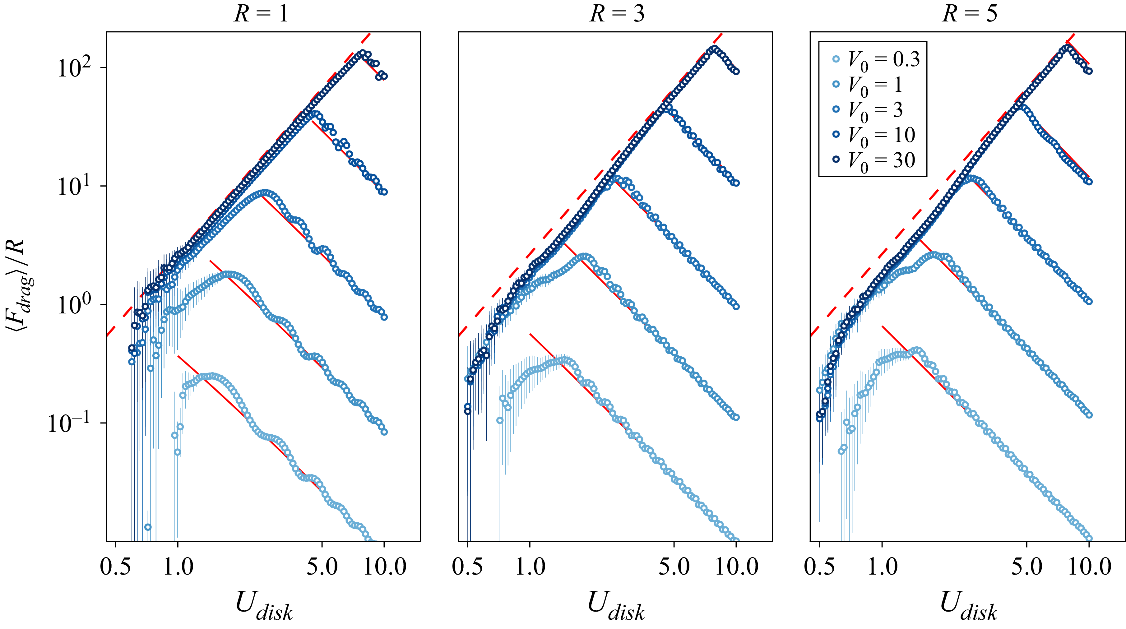
Rescaled steady-state time-averaged drag,
 $\langle F_{\textit{drag}}\rangle /R$
, versus disk speed,
 $U_{\textit{disk}}$
. Standard deviation bars, as per Appendix C.4, indicate unsteadiness in
 $F_{\textit{drag}}$
for
 $U_{\textit{disk}} \lesssim 1.5$
. Equation (4.9) for an impenetrable disk (dashed red line) and (4.10) for a highly penetrable disk (red lines). Data reported only when excitations such as vortices are emitted from the disk in steady state, giving non-zero drag. Computational parameters are as for figure 2.

Complementary results for a (subsonic) disk speed of
 $U_{\textit{disk}} = 0.7$
are reported in figure 6. Here, the analytical theory in § 4 predicts that disk penetrability will be manifest when
 $V_0 \lesssim (1/2) U_{\textit{disk}}^2 = 0.245$
for
 $U_{\textit{disk}} = 0.7$
. This agrees with the numerical results in figure 6, with wakes for
 $V_0 \geqslant 1$
being similar in structure and number density distribution; this is particularly evident in the level sets in figure 6(b), which are similar in form. However, the wake changes substantially for a penetrable disk with
 $V_0 = 0.3$
(at
 $U_{\textit{disk}} = 0.7$
), resembling that for an impenetrable disk moving at the slower speed of
 $U_{\textit{disk}} = 0.5$
, cf. the first row of figure 2 and the fourth row of figure 6. Moreover, discrete vortices (with zero density at their cores) also occur for
 $V_0 = 0.3$
, as evidenced by the level sets (ninth row of figure 6) being (i) of similar size to those for larger
 $V_0$
, and (ii) aligning with the corresponding density disturbances (fourth row of figure 6). They also exhibit a quantised circulation of
 $\pm 2\pi$
(data not shown). Reducing the barrier height to
 $V_0 = 0.1$
quenches vortex generation. This agrees with studies showing a barrier height,
 $V_0 \lt 1$
, can increase the critical disk speed,
 $U_{\textit{critical}}$
, for the onset of vortex shedding relative to the impenetrable case,
 $V_0 \gg 1$
(Kwon et al. Reference Kwon, Moon, Seo and Shin2015; Huynh et al. Reference Huynh, Hébert, Albert and Larré2024). Results for disk radii of
 $R = 1$
and
 $5$
are reported in figures S3–S6 of the supplementary material.
In summary, these results show that the vortex wake generated by a penetrable disk moving at subsonic speed can resemble that of an impenetrable disk moving at slower speed. The same is not true for disks moving at supersonic speeds, where the wake morphology can significantly differ from that of an impenetrable disk.
6.2.2. Steady-state time-averaged drag
We now examine the steady-state time-averaged drag,
 $\langle F_{\textit{drag}}\rangle$
, experienced by a moving disk. Figure 7 gives this drag computed from DNS of (2.20) as a function of the disk’s speed,
 $U_{\textit{disk}}$
, radius,
 $R$
, and barrier height,
 $V_0$
. The asymptotic formula for an impenetrable disk moving at high speed, (4.9), is included in figure 7 (dashed red line of positive slope), with its linear dependence on the disk radius,
 $R$
, used to scale all results. The complementary asymptotic formula for a highly penetrable disk, (4.10), is also shown (solid red line of negative slope).
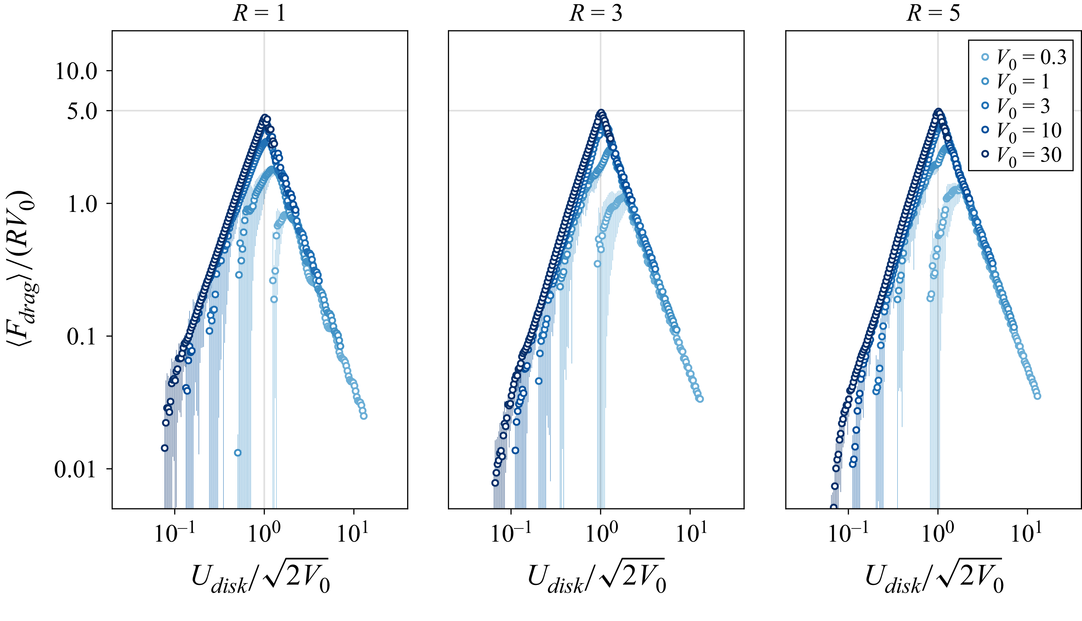
A striking feature of the drag in figure 7 for a penetrable disk is its unimodal dependence on disk speed,
 $U_{\textit{disk}}$
, for all disk radii,
 $R = 1$
,
 $3$
and
 $5$
. This is consistent with the theoretical prediction in § 4.3. It differs from the drag experienced by an impenetrable disk, which increases monotonically for all disk speeds,
 $U_{\textit{disk}}$
. The drag in figure 7 is observed to increase monotonically and match (4.9) for an impenetrable disk when
 $1 \ll U_{\textit{disk}} \ll \sqrt {2 V_0}$
; because
 $R \geqslant 1$
, this corresponds to the classical regime,
 $U_{\textit{disk}} R \gg 1$
, as required. For larger disk speeds, a maximum drag,
 $F_{\textit{drag}}^{\textit{max}}$
, exists for each barrier height,
 $V_0$
. The maximum drag is observed to increase with
 $V_0$
. This finding is in qualitative agreement with the scaling relation in (4.11), derived using asymptotic drag formulas for an impenetrable disk, (4.9), and a highly penetrable disk, (4.10), moving at high speed. It also agrees with the exact solution to the linear Schrödinger equation; see Appendix D.1. Note that the maximum drag in figure 7 predominantly occurs at supersonic speeds, where the instantaneous drag is steady; see § 6.1.2. This is evidenced by small or imperceivable standard deviation bars in figure 7 at the maximum drag. Equation (4.10) agrees with the DNS data in its regime of validity, i.e.
 $1 \ll \sqrt {2 V_0} \ll U_{\textit{disk}}$
and
 $U_{\textit{disk}} R \gg 1$
. This validates the asymptotic formula, (4.10), for a highly penetrable disk that can evidently be used with confidence to calculate the drag in this limit.
The scaled drag is found to be of similar form and magnitude for the three disk radii studied,
 $R = 1$
,
 $3$
and
 $5$
. It exhibits oscillations as a function of the disk speed,
 $U_{\textit{disk}}$
, in the highly penetrable disk regime. This is most pronounced for the smallest disk radius of
 $R = 1$
and increases in frequency with disk radius. These oscillations arise from the quantum wave nature of the flow that depend on the dimensionless wavenumber,
 $U_{\textit{disk}} R$
. Results for
 $R=3$
and
 $5$
correspond to higher values of
 $U_{\textit{disk}} R$
, where the oscillations decrease in magnitude and vanish in the limit,
 $U_{\textit{disk}} R \to \infty$
, as shown in Appendix A.
Data from figure 7, plotted as the rescaled force,
 $\langle F_{\textit{drag}}\rangle /(R V_0)$
, versus the rescaled disk speed,
 $U_{\textit{disk}} / \sqrt {2 V_0}$
.

6.2.3. Maximum drag
Next, we assess the validity of the high-speed, maximum drag scaling formula in (4.11). This formula predicts that the maximum drag scales with the product,
 $R V_0$
, and is derived by noting that the penetrable and impenetrable disk regimes are delineated by the condition,
 $U_{\textit{disk}} \sim \sqrt {2 V_0}$
, i.e. they depend on the ratio,
 $U_{\textit{disk}}/\sqrt {2 V_0}$
. Because (4.11) is derived for
 $U_{\textit{disk}}\gg 1$
, it is expected to hold provided
 $V_0 \gg 1$
. Rescaling the data in figure 7 accordingly gives the results in figure 8, which indeed appear to exhibit a maximum drag as
 $V_0$
increases.
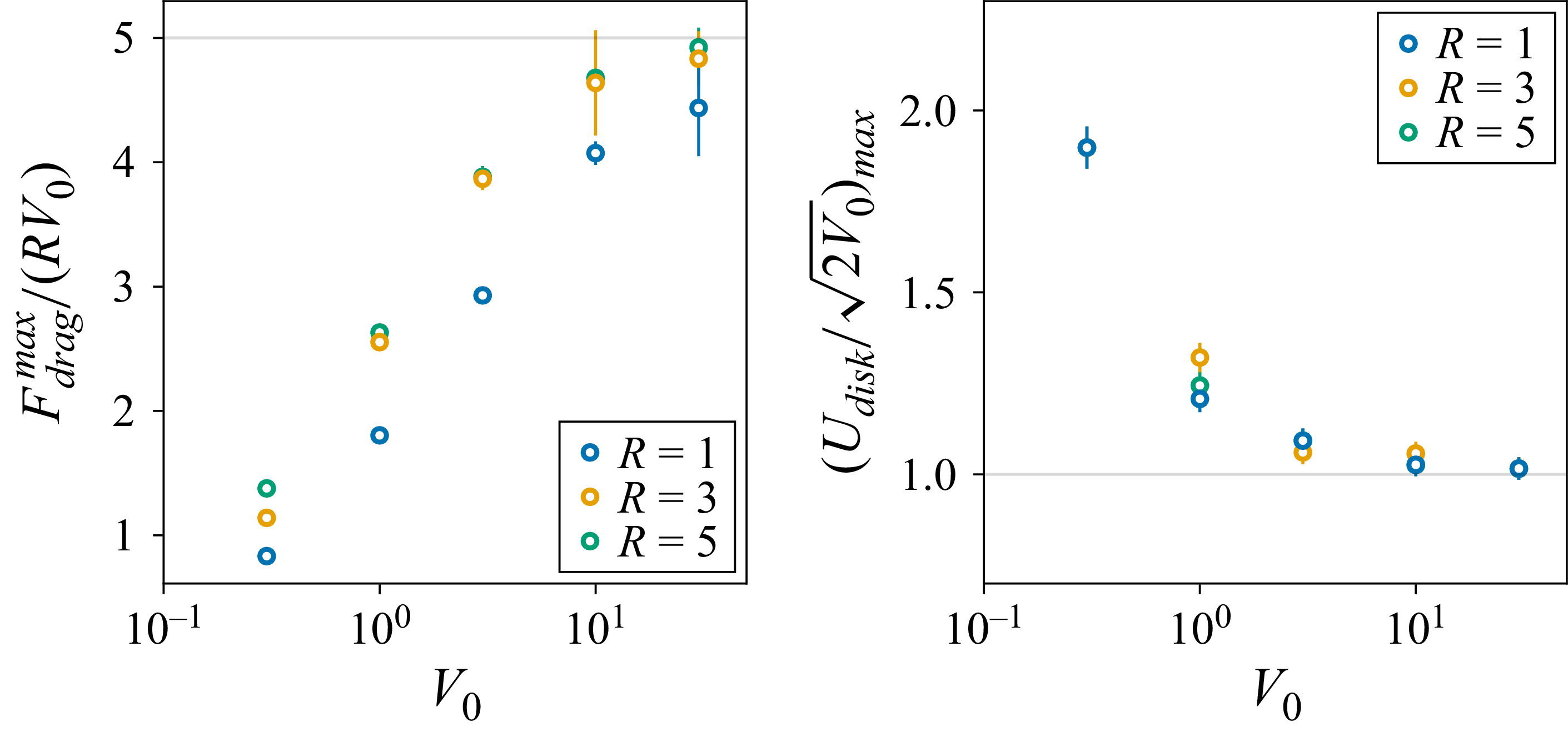
Maximum rescaled drag,
 $ F_{\textit{drag}}^{\textit{max}} /(R V_0)$
, and the rescaled disk speed,
 $[U_{\textit{disk}} / \sqrt {2 V_0}]_{\textit{max}}$
, at which it occurs, as a function of the disk barrier height,
 $V_0$
, and radius,
 $R$
. Results are derived from data in figure 8. Error bars are one standard error as per Appendix C.4.

The position of maximum drag for
 $V_0 \gg 1$
is found to occur very close to
 $U_{\textit{disk}} = \sqrt {2 V_0}$
; see the vertical grey line that is plotted precisely at
 $U_{\textit{disk}} /\sqrt {2 V_0} = 1$
in figure 8. Horizontal grey lines are at a single rescaled drag value, which highlights the insensitivity of the maximum rescaled drag for
 $R \geqslant 1$
and
 $V_0 \gg 1$
; a small decrease in the maximum rescaled drag is observed for
 $R = 1$
. Figure 9 gives the variation in the maximum drag and the value of
 $U_{\textit{disk}} /\sqrt {2 V_0}$
at which it occurs as a function of the disk barrier height,
 $V_0$
, and disk radius,
 $R$
. This data indicates a general convergence to a maximum drag given by
 \begin{equation} F_{\textit{drag}}^{\textit{max}} \approx 5 R V_0 \quad \text{at} \ U_{\textit{disk}} \approx \sqrt {2 V_0}, \end{equation}
for
 $V_0 \gg 1$
and
 $R \geqslant 1$
. This implicitly holds for a high disk speed,
 $U_{\textit{disk}} \gg 1$
, in the classical regime,
 $U_{\textit{disk}} R \gg 1$
. We emphasise that (6.1) is an empirical result derived from numerical data and its mathematical verification remains an avenue for future work.
6.2.4. Disk motion under an applied force
The steady-state time-averaged drag experienced by a disk moving at constant velocity is reported in the previous sections. Here, we consider the complementary case of a penetrable disk moving under a constant externally applied force,
 $F_{\textit{applied}}$
. This situation could conceivably be achieved in a Bose–Einstein condensate by moving a laser spot under load control. This behaviour is modelled by assuming the drag experienced by the disk can be approximated by the steady-state drag calculated above. While an impenetrable disk under a constant applied force and steady drag will move at a well-defined speed in steady state, the resulting motion of a penetrable disk is more complex. This difference arises from the unimodal nature of the drag with respect to the disk speed. We consider supersonic disk speeds in the classical limit, where the drag is steady.
(a–c) Phase diagrams for the dynamical system describing the motion of a penetrable disk under a constant applied force:
 $\textrm{d} U_{\textit{disk}} / \textrm{d}t = F_{\textit{applied}} - F_{\textit{drag}} (U_{\textit{disk}})$
, where time is normalised by the effective disk mass. Drag law is represented as a ‘V’ curve for simplicity. A saddle-node bifurcation occurs when
 $F_{\textit{applied}} = F_{\textit{drag}}^{\textit{max}}$
. Disk trajectories are indicated by arrows on the horizontal axis; circles are equilibria. Here, filled circles denote a stable equilibrium, open circles an unstable equilibrium, and half-filled circles a semi-stable equilibrium.

Three scenarios exist that are dictated by the magnitude of the applied force,
 $F_{\textit{applied}}$
, relative to the maximum drag,
 $F_{\textit{drag}}^{\textit{max}}$
, for a given barrier height,
 $V_0$
. Specifically, when the applied force is
-
(i) greater than the maximum drag,
$F_{\textit{applied}} \gt F_{\textit{drag}}^{\textit{max}}$
; -
(ii) precisely equal to the maximum drag,
$F_{\textit{applied}} = F_{\textit{drag}}^{\textit{max}}$
; and -
(iii) less than the maximum drag,
$F_{\textit{applied}} \lt F_{\textit{drag}}^{\textit{max}}$
.


These three scenarios are illustrated in figure 10 with their corresponding dynamical system described in its caption. A saddle-node bifurcation evidently occurs when
 $F_{\textit{applied}} = F_{\textit{drag}}^{\textit{max}}$
; see figure 10(b).
In the first scenario (figure 10 a), the disk accelerates unboundedly because the drag exerted by the fluid cannot balance the applied force. The second scenario (figure 10 b) is more complex with a bifurcation corresponding to the appearance of a single equilibrium disk speed. A disk moving at a speed below this equilibrium speed will accelerate until it reaches the equilibrium speed. However, if the disk is already moving faster than the equilibrium speed, it will accelerate unboundedly, i.e. the equilibrium speed is semi-stable.
Under the third scenario (figure 10
c), two equilibrium speeds exist: one less than and one greater than the disk speed for maximum drag, denoted
 $U_{\textit{disk}}^{{low}}$
and
 $U_{\textit{disk}}^{{high}}$
, respectively. If the disk is started at a speed below
 $U_{\textit{disk}}^{{low}}$
, it will accelerate to
 $U_{\textit{disk}}^{{low}}$
. Similarly, if the force is applied to a disk already moving at a speed between
 $U_{\textit{disk}}^{{low}}$
and
 $U_{\textit{disk}}^{{high}}$
, it will decelerate to
 $U_{\textit{disk}}^{{low}}$
, i.e.
 $U_{\textit{disk}}^{{low}}$
is a stable equilibrium. However, if the force is applied to a disk moving at a speed exceeding
 $U_{\textit{disk}}^{{high}}$
, it will accelerate unboundedly, i.e. motion at
 $U_{\textit{disk}}^{{high}}$
is unstable. These theoretical predictions await substantiation through experimental measurement.
7. Conclusions
The drag experienced by a penetrable disk that is moving in a superfluid, whose dynamics are specified by the GP equation, has been studied. This models the force exerted by a moving laser spot on a weakly interacting Bose–Einstein condensate. This drag depends on three dimensionless parameters: the scaled disk radius,
 $R$
, disk speed,
 $U_{\textit{disk}}$
, and barrier height,
 $V_0$
.
The study was performed by first considering the asymptotic limits of impenetrable and highly penetrable disks, for which analytical formulas were reported in the high-speed limit. These formulas suggest that the drag depends on disk speed in a unimodal fashion. Maximum drag occurs when the disk barrier height matches the relative kinetic energy of the fluid, i.e. its chemical potential in the moving frame of the disk. These results were used to derive a scaling relation showing that the maximum drag varies with the product of the disk radius and barrier height.
The flow generated by a moving penetrable disk was then determined by DNS of the GP equation. Well-known features of the wake generated by an impenetrable disk were recovered and compared with those for a penetrable disk, as the barrier height was varied. These results showed that the wakes generated by a penetrable disk moving at subsonic speeds are similar to those of an impenetrable disk moving at a slower speed. However, a penetrable disk moving at supersonic speed generates a wake that can substantially differ from that of an impenetrable disk. High disk penetrability generates small density disturbances in the fluid at supersonic disk speeds, which are not found for impenetrable disks.
Direct numerical solution confirmed the above-mentioned theoretical prediction that the drag experienced by a penetrable disk is a unimodal function of its speed. This numerical data validated the above-mentioned formulas for impenetrable and highly penetrable disks, the derived scaling relation for the maximum drag, and the disk speed at which it occurs. This holds provided (i) the barrier height greatly exceeds the chemical potential of the stationary fluid, and (ii) the disk radius is much larger than the quantum healing length. The dimensionless maximum drag was found to be
 $F_{\textit{drag}}^{\textit{max}} \approx 5 R V_0$
and occurs when
 $U_{\textit{disk}} \approx \sqrt {2 V_0}$
under these conditions.
The unimodal nature of the drag was shown to yield tuneable dynamics for a penetrable disk moving under a constant applied force. This motivates new laser experiments on Bose–Einstein condensates and their applications in quantum technologies.
Supplementary material and movies
Supplementary material and movies are available at https://doi.org/10.1017/jfm.2026.11467.
Funding
The authors acknowledge support from the Gary Clinard Innovation Fund.
Declaration of interests
The authors report no conflict of interest.
Appendix A. Drag experienced by a highly penetrable disk
We analytically calculate the drag experienced by a highly penetrable disk, i.e.
 $U_{\textit{disk}}^2 \gg 2 V_0$
, in the classical limit,
 $U_{\textit{disk}} R \gg 1$
. This is achieved by solving (4.5) using the Born approximation in the weak scattering limit (Griffiths & Schroeter Reference Griffiths and Schroeter2018).
In this highly penetrable disk limit,
 $f(\theta )$
is calculated to leading order using the first Born approximation to (4.5) giving
 \begin{equation} f(\theta ) = - \sqrt {\frac {\pi }{2}} R V_0 U_{\textit{disk}}^{-\frac {3}{2}} \frac {J_1 \! \left (2 U_{\textit{disk}} R \sin \! \left (\dfrac {\theta }{2}\right ) \right )}{\sin \! \left (\dfrac {\theta }{2}\right )}, \end{equation}
where
 $J_1(.)$
is the Bessel function of first order. Substituting (A1) into (4.8), and changing variable to
 $s = \sin (\theta /2)$
, gives
 \begin{equation} \sigma = \frac {4 \pi R^2 V_0^2}{U_{\textit{disk}}^3} \int _0^1 \frac {J_1^2 (2 U_{\textit{disk}} R s)}{\sqrt {1-s^2}} \, {\rm d}s. \end{equation}
The integral in (A2) can be evaluated analytically, giving
 \begin{equation} \int _0^1 \frac {J_1^2 (2 U_{\textit{disk}} R s)}{\sqrt {1-s^2}} \, {\rm d}s = \frac {\pi (U_{\textit{disk}} R)^2}{4} {}_2 F_3 \! \left ( \frac {3}{2}, \frac {3}{2}; 2, 2, 3; -4(U_{\textit{disk}} R)^2 \right )\!, \end{equation}
where
 ${}_2 F_3$
is a generalised hypergeometric function. Substituting (A3) into (A2) and (4.7) then gives the force
 \begin{equation} F_{\textit{drag}} = \pi ^2 R^4 V_0^2 U_{\textit{disk}} \left [ {}_2 F_3 \! \left ( \frac {3}{2}, \frac {3}{2}; 2, 2, 3; -4 (U_{\textit{disk}} R)^2 \right ) \right ]\!, \end{equation}
which is valid for arbitrary
 $U_{\textit{disk}} R$
, under the above-imposed constraint of
 $U_{\textit{disk}} \gg 1$
.
Expanding the hypergeometric function for
 $U_{\textit{disk}} R\gg 1$
then yields the required expression for the drag experienced by a highly penetrable disk in the classical limit,
 \begin{align} F_{\textit{drag}} &= 2 R \left ( \frac {V_0}{U_{\textit{disk}}} \right )^2 \big [ 5 \log 2 -2 + \gamma + \log \! \left ( U_{\textit{disk}} R \right ) \! \big ]\nonumber \\ & \approx 2 R \left ( \frac {V_0}{U_{\textit{disk}}} \right )^2 \log \! \left (7.713 \, U_{\textit{disk}} R\right ), \quad U_{\textit{disk}} R \gg 1, \end{align}
where
 $\gamma = 0.5772\ldots$
is Euler’s constant.
Appendix B. Drag experienced by a disk of arbitrary penetrability
The drag according to (4.5) that is experienced by a disk of arbitrary barrier height,
 $V_0$
, can be calculated using a general eigenfunction expansion (Griffiths & Schroeter Reference Griffiths and Schroeter2018). The formalism in § 4 then gives
 \begin{equation} F_{\textit{drag}} = 2 U_{\textit{disk}} \! \sum _{m=-\infty }^{\infty }\sin ^2\!\big (\delta _{m+1}-\delta _m\big ), \end{equation}
where the phase,
 $\delta _m$
, is defined by
 \begin{equation} \tan \delta _m = \left \{ \begin{array}{ll}\displaystyle \frac {\alpha J_m'(\alpha \kappa ) J_m(\kappa ) - J_m(\alpha \kappa ) J_m'(\kappa )} {\alpha J_m'(\alpha \kappa ) Y_m(\kappa ) - J_m(\alpha \kappa ) Y_m'(\kappa )}, & U_{\textit{disk}}^2 \gt 2 V_0, \\ \\ \displaystyle \frac {\beta I_m'(\beta \kappa ) J_m(\kappa ) - I_m(\beta \kappa ) J_m'(\kappa )} {\beta I_m'(\beta \kappa ) Y_m(\kappa ) - I_m(\beta \kappa ) Y_m'(\kappa )}, & U_{\textit{disk}}^2 \lt 2 V_0,\end{array}\right . \end{equation}
with the dash
 $'$
denoting the derivative,
 $Y_m(.)$
is the Bessel function of the second kind,
 $I_m(.)$
is the modified Bessel function of the first kind and
 \begin{equation} \alpha = \sqrt {1- \frac {2 V_0}{U_{\textit{disk}}^2}}, \quad \beta = \sqrt {\frac {2 V_0}{U_{\textit{disk}}^2}-1}, \quad \kappa = U_{\textit{disk}} R. \end{equation}
The infinite sum in (B1) is truncated for numerical evaluation, i.e.
 \begin{equation} F_{\textit{drag}} = 2 U_{\textit{disk}} \! \sum _{m=-M}^{M}\sin ^2\!\big (\delta _{m+1}-\delta _m\big ), \end{equation}
with
 $M$
increased until convergence is achieved. This parameter is found to scale as
 $M \sim \kappa$
for
 $\kappa = U_{\textit{disk}} R \gg 1$
, corresponding to the classical limit.
Appendix C. Numerical method to solve the GP equation
The wavefunction,
 $\psi$
, satisfying the GP equation (2.1), is computed numerically on a finite spatial domain in the Cartesian
 $x$
–
 $y$
frame using a split-time Fourier method (Fiet, Fleck & Steiger Reference Fiet, Fleck and Steiger1982). The spatial derivatives are evaluated using the discrete Fourier transform, which yields spectral accuracy, while the external potential,
 $V_{\textit{ext}}$
, is integrated using a mid-point rule to ensure overall second-order accuracy in time. Accordingly, the wavefunction,
 $\psi$
, is time stepped using
 \begin{align} \psi (\boldsymbol{r}, t+\Delta t) &= \mathcal{F}^{-1} \! \left \{ \exp \left (- \frac {i}{2} K^2 \Delta t \right ) \right . \nonumber \\ & \times \left . \mathcal{F} \! \left \{ \exp \left ( -i \left [ V_{\textit{ext}} \! \left (\boldsymbol{r}, t+ \frac {\Delta t}{2}\right ) + \big | \psi (\boldsymbol{r}, t) \big |^2 \right ] \Delta t \right ) \psi (\boldsymbol{r}, t) \right \} \right \} + O \big ( \Delta t^3 \big ), \end{align}
where
 $\Delta t$
is the time step,
 $\mathcal{F}$
denotes the (spatial) discrete Fourier transform with
 $\mathcal{F}^{-1}$
being its inverse, whereas the wavenumber matrix,
 $K^2 = [ K_{\textit{mn}}^2 ]$
, for this two-dimensional problem has the elements,
 \begin{equation} K_{\textit{mn}}^2 = \left [ \left (\frac {\pi m}{L_x}\right )^2 + \left (\frac {\pi n}{L_y}\right )^2 \right ]\!, \quad m = 0,\ldots , N_x - 1; \, \, n = 0,\ldots , N_y - 1, \end{equation}
with
 $L_x$
and
 $L_y$
being the respective lengths of the spatial domain in the
 $x$
and
 $y$
directions;
 $N_x$
and
 $N_y$
are the corresponding number of grid points. Note that the (numerical) wavenumber matrix is unrelated to the quantum wavenumber,
 $k$
, in (3.1). The discrete cosine transform is used to ensure the wavefunction has zero gradient at the boundary of the spatial computational domain.
C.1. Ground state
The flow problem is initialised in the ground state of the superfluid, with the external potential for the circular disk in its initial stationary position. This ground state is computed using the ‘imaginary time evolution’ method that involves replacing
 $i \to 1$
on the left-hand side of (2.20) (Chiofalo, Succi & Tosi Reference Chiofalo, Succi and Tosi2000). The resulting equation is solved using a modification of (C1) under the same replacement, i.e.
 $i \to 1$
. The number of particles in the flow domain is fixed, i.e.
 \begin{equation} \frac {1}{V} \int _V |\psi |^2 \, {\rm d}V = 1, \end{equation}
which is enforced by rescaling the wavefunction at each time step.
C.2. External circular disk potential
The external potential used for a circular disk of radius,
 $R$
, moving with velocity,
 $U_{\textit{disk}}$
in the
 $x$
direction, is the step function,
 \begin{equation} V_{\textit{ext}} (\boldsymbol{r}, t) = V_{\textit{ext}} (x, y, t) = V_0 \, H \! \left ( 1- \frac {(x - U_{\textit{disk}} \, t)^2 + y^2}{R^2} \right )\!, \end{equation}
where
 $H$
is the Heaviside function and
 $V_0$
is the barrier height.
C.3. Force calculation
Equation (2.7) shows that the disk external potential,
 $V_{\textit{ext}}$
, exerts a body force on the fluid. Newton’s third law then establishes that the force exerted by the superfluid on the disk is
 \begin{equation} \boldsymbol{F} = \int _V n \, \boldsymbol{\nabla }V_{\textit{ext}} \, {\rm d}V, \end{equation}
and the integration domain is where
 $V_{\textit{ext}}$
exhibits spatial gradients. This equation simplifies for an external potential,
 $V_{\textit{ext}}$
, with a constant (finite) barrier height of
 $V_0$
in its interior and zero outside; as in (C4). For such a potential of arbitrary shape, (C5) becomes
 \begin{equation} \boldsymbol{F} = - V_0 R \int _{\partial V} \! \! n \, \hat {\boldsymbol{n}} \, {\rm d} S, \end{equation}
where
 $\hat {\boldsymbol{n}}$
(not to be confused with
 $n$
) is the outward unit normal vector to the interior of
 $V_{\textit{ext}}$
and
 $\partial V$
denotes the boundary of the integration domain in (C5).
Equations (C4) and (C6) then give the required drag per unit length,
 $F_{\textit{drag}} = - \hat {\boldsymbol{x}} \boldsymbol{\cdot }\boldsymbol{F}$
, experienced by a disk, where
 $\hat {\boldsymbol{x}}$
is the Cartesian basis vector in the
 $x$
direction, with
 \begin{equation} F_{\textit{drag}} = V_0 R \int _0^{2 \pi } \! \! n |_{r = R} \cos \theta \, {\rm d} \theta , \end{equation}
in polar coordinates,
 $(r, \theta )$
, centred on the disk, with
 $\theta = 0$
coinciding with the
 $x$
direction (as above). The number density on the disk boundary is needed to evaluate (C7). This is calculated by interpolating the number density values computed on the rectangular spatial grid using cubic splines.
C.4. Vortex shedding frequency and steady-state time-averaged drag
Vortices in a superfluid are characterised by two features: (i) the superfluid density is zero at the centre of each vortex, and (ii) the circulation around a loop enclosing a single vortex is non-zero (quantised in units of
 $2\pi$
; see § 2.2). This enables determination of the number of vortices in a superflow via the total shed circulation, which is computed using a two-step process. First, we identify ‘contiguous regions’ (defined in the next paragraph) where the number density,
 $n$
, is below a user-defined threshold: we choose a nominal value of
 $n_{\textit{thres}} = 0.03$
in all numerical results. Second, we compute the circulation of each region by integrating the fluid velocity around the region boundary. The ‘total shed circulation’ of these regions,
 $\varGamma _{\textit{regions}}$
, is obtained by summing the magnitude of the circulation around each region.
A contiguous region is a collection of adjacent grid points in the computational spatial domain (nearest neighbours, including diagonals) where each grid point has a density,
 $n \lt n_{\textit{thres}}$
. The contiguous regions can be computed via a depth-first traversal of the grid points, visiting the neighbours of grid points below
 $n_{\textit{thres}}$
, and tracking grid points already visited. We ignore the contiguous region formed around the aerofoil where
 $n \lt n_{\textit{thres}}$
.
The total shed circulation of these regions,
 $\varGamma _{\textit{regions}}$
, is calculated at each time step from which the rate of vortex formation,
 $1/(2 \pi ) {\rm d} \varGamma _{\textit{regions}}/{\rm d}t$
, i.e. the vortex shedding frequency, is computed by linear regression. Estimating the number of vortices solely by counting the total number of contiguous regions,
 $N_{\textit{regions}}$
, can systematically overestimate the number of vortices and thereby the rate of vortex formation; see Appendix E. This overestimation is caused by the formation of flow structures with a small number density but no net circulation. Finally, we note that use of a moving disk in an otherwise quiescent fluid ensures that all shed vortices remain in the flow domain. This eliminates the need to remove vortices as they exit the flow domain, as would otherwise be required.
The steady-state time-averaged drag,
 $\langle F_{\textit{drag}} \rangle$
, and vortex shedding frequency,
 $1/(2 \pi ) {\rm d} \varGamma _{\textit{regions}}/{\rm d}t$
, generated by the disk are computed using data from the second half of each DNS run, i.e. after transients from start up have decayed and before wave reflection from the spatial domain boundary significantly affect the results. Standard deviation bars for
 $\langle F_{\textit{drag}} \rangle$
in figure 7, 11–13 are used to show when (i) the steady-state drag is time dependent, and (ii) the numerical artefact discussed in Appendix D.2 is prevalent. Error bars associated with the vortex shedding frequency,
 $1/(2 \pi ) {\rm d} \varGamma _{\textit{regions}}/{\rm d}t$
, in figure 16 are the standard error arising from linear regression.
Appendix D. Benchmarking and convergence studies
Convergence studies of the numerical method described in § 5 and Appendix C and its benchmarking are reported here.
Linear Schrödinger equation for high disk speed. Black line: exact formula, (B4), for arbitrary penetrability,
 $U_{\textit{disk}}^2 /(2 V_0)$
, and wavenumber,
 $U_{\textit{disk}} R$
. Red dashed line (positive slope): impenetrable formula, (4.9), for
 $U_{\textit{disk}}^2 \ll 2 V_0$
and
 $U_{\textit{disk}} R \gg 1$
. Red line (negative slope): highly penetrable formula, (A5), for
 $U_{\textit{disk}}^2 \gg 2 V_0$
and
 $U_{\textit{disk}} R \gg 1$
. Blue circles: DNS of (4.1) with standard deviation bars as per Appendix C.4. Computational parameters:
 $R=1$
,
 $L=128$
and
 $\Delta t$
as per (5.4); reducing
 $L$
by a factor of two does not affect the results (data not shown).

Convergence of steady-state time-averaged drag,
 $\langle F_{\textit{drag}} \rangle$
, for a disk of radius,
 $R=3$
, versus disk speed,
 $U_{\textit{disk}}$
, as a function of the domain size,
 $L$
. Results are shown for (a)
 $\Delta x = 1/4$
and (b)
 $\Delta x = 1/8$
. Insets give results for low disk speeds. Equation (4.9) is shown as a red line. Standard deviation bars as per Appendix C.4. Computational parameters:
 $V_0 = 30$
and
 $\Delta t$
as per (5.4).

(a) Convergence of the steady-state time-averaged drag for a disk of radius,
 $R=3$
, and (b) corresponding time series for the instantaneous drag for
 $U_{\textit{disk}} = 3.8$
, as the grid size,
 $\Delta x$
, is varied. Standard deviation bars as per Appendix C.4. A reduced sample dataset of three points is shown for
 $\Delta x = 1/16$
, due to computational expense. Computational parameters:
 $V_0 = 30$
,
 $L = 256$
and
 $\Delta t$
as per (5.4).

D.1. Linear Schrödinger equation
The numerical method is first used to calculate the steady-state drag experienced by a disk of radius,
 $R=1$
, according to the linear Schrödinger equation in (4.1). Its results are given in figure 11 for three dimensionless wavenumbers,
 $U_{\textit{disk}} R = 1$
,
 $3$
and
 $10$
. Each column of figure 11 corresponds to a single disk speed,
 $U_{\textit{disk}} = 1$
,
 $3$
and
 $10$
, where the barrier height,
 $V_0$
, is varied in each subplot. Data derived from DNS of (4.1) are compared with (i) the exact analytical solution in (B1), and (ii) asymptotic formulas for disks of low and high penetrability, reported in (4.9) and (A5), respectively. The asymptotic formulas agree with (B1) in their respective limits. This comparison provides an independent means of assessing the validity of the numerical method by using an exact analytical solution.
The DNS data in figure 11 are observed to converge to the exact analytical solution with decreasing
 $\Delta x$
. Convergence is most rapid for the smallest wavenumber,
 $U_{\textit{disk}} R = 1$
, i.e. the lowest disk speed, with a finer grid required for the largest wavenumber of
 $U_{\textit{disk}} R = 10$
, i.e. the highest disk speed. This is expected because the quantum wavelength decreases with increasing wavenumber. The true steady-state drag experienced by the disk is steady at all disk speeds, according to the linear Schrödinger equation (4.1). The reported standard deviation bars are thus due to numerical error, which decreases with spatial grid refinement; this effect is investigated in more detail in Appendix D.2 for the GP equation.
D.2. Computational grid and domain sizes
We now examine convergence of the steady-state time-averaged drag,
 $\langle F_{\textit{drag}}\rangle$
, according to the GP equation (2.20), as the computational parameters are varied. These results are benchmarked against equivalent numerical data reported by Winiecki et al. (Reference Winiecki, McCann and Adams1999).
Comparison to figure 3 of Winiecki et al. (Reference Winiecki, McCann and Adams1999): we first consider an impenetrable disk of radius,
 $R=3$
, to enable comparison with figure 3 of Winiecki et al. (Reference Winiecki, McCann and Adams1999), where the time-averaged drag,
 $\langle F_{\textit{drag}} \rangle$
, versus disk speed,
 $0\lt U_{\textit{disk}} \leqslant 4$
, was reported. Winiecki et al. (Reference Winiecki, McCann and Adams1999) used an identical non-dimensionalisation to § 2.3 but with the Crank–Nicolson method to solve (2.20) for a moving circular disk. This employed a time step of
 $0.01$
and a
 $200\times 200$
square computational domain that was divided into
 $800 \times 800$
points, giving a spatial grid discretisation of
 $1/4$
. Winiecki et al. (Reference Winiecki, McCann and Adams1999) used an absorbing layer near the domain boundary to minimise wave reflection; this is not implemented here. That previous study also defined the disk using a moving external potential. While the barrier height,
 $V_0$
, was not specified, it was stated that the time-averaged drag is weakly dependent on the barrier height for
 $V_0 \gt 1$
. Given the findings in § 4, we choose
 $V_0 = 30 \, [\gg \! (1/2) U_{\textit{disk}}^2]$
to reproduce the data in figure 3 of Winiecki et al. (Reference Winiecki, McCann and Adams1999).
Figure 12(a) gives the steady-state time-averaged drag,
 $\langle F_{\textit{drag}} \rangle$
, using
-
(i)
$N=1025$
,
$L = 256$
and
$\Delta x = 1/4$
(
$\alpha = 10$
and
$\beta = 2$
) with
$\Delta t \approx 0.0063$
to mimic Winiecki et al. (Reference Winiecki, McCann and Adams1999), giving a domain-size to disk-radius ratio of
$L/R \approx 85$
; and -
(ii) double this domain size for the same grid discretisation, i.e.
$N=2049$
,
$L = 512$
and
$\Delta x = 1/4$
(
$\alpha = 11$
and
$\beta = 2$
) giving
$L/R \approx 171$
, to reduce boundary effects (if any).


Figure 12(b) reports results for
 $\Delta x = 1/8$
with the same domain sizes, i.e. the spatial grid size is halved. All other computational parameters are specified above. The high-speed formula for an impenetrable disk, (4.9), is also reported as in figure 3 of Winiecki et al. (Reference Winiecki, McCann and Adams1999), facilitating comparison; identical horizontal and vertical axes scales are used.
The results in figure 12(a) show that doubling the computational domain, while retaining the same grid discretisation, has no perceivable effect on
 $\langle F_{\textit{drag}} \rangle$
within the standard deviation bars. Refining the grid discretisation by a factor of two is found to dramatically reduce the standard deviation bars, while maintaining similar mean values; see figure 12(b). This reduction in numerical error is commensurate with the results in figure 11 for the linear Schrödinger equation. The onset of drag at low disk speed (see insets of figure 12) is observed to occur at
 $U_{\textit{disk}} \approx 0.4 - 0.5$
, in agreement with figure 3 of Winiecki et al. (Reference Winiecki, McCann and Adams1999) and other literature results for impenetrable disks (Huepe & Brachet Reference Huepe and Brachet2000). However, the results at high disk speed agree more closely with (4.9) than in figure 3 of Winiecki et al. (Reference Winiecki, McCann and Adams1999). The reason for this difference is unclear for several possible reasons, including the use of different numerical methods. It may also be related to the choice of barrier height,
 $V_0$
, which was not reported by Winiecki et al. (Reference Winiecki, McCann and Adams1999), and insufficient grid discretisation.
Figure 13 gives results as the grid discretisation,
 $\Delta x$
, is varied. This is performed at a high disk speed, which is the speed range where the above-mentioned discrepancy with figure 3 of Winiecki et al. (Reference Winiecki, McCann and Adams1999) is observed. The steady-state time-averaged drag (panel a) and sample time series for the instantaneous drag (panel b) are reported. These results show that grid discretisations of
 $\Delta x = 1/2$
and
 $1/4$
do not lead to converged results with a significant numerical error; the data are insensitive to domain size,
 $L$
, as in figure 12. Data for
 $\Delta x = 1/2$
and
 $1/4$
exhibit a spurious oscillatory time dependence, which is resolved upon grid refinement to
 $\Delta x = 1/8$
; these spurious effects are investigated further below. Reducing the grid size to
 $\Delta x = 1/16$
gives results that agree with those for
 $\Delta x = 1/8$
, indicating convergence.
Regularisation of the disk potential,
 $V_{\textit{ext}}$
, to reduce the above-mentioned numerical artefacts, e.g. by smoothing its step discontinuity, is not used. This is because this regularisation (i) alters the flow problem, and (ii) decreases convergence of the computed force as the grid spacing,
 $\Delta x$
, is reduced, in the highly penetrable disk limit (data not shown). The computational parameters,
 $\alpha$
and
 $\beta$
, are therefore adjusted so that numerical artefacts do not significantly affect the generated data in § 6. Reducing the time step,
 $\Delta t$
, by a factor of two in the above studies has no perceivable effect, establishing that (5.4) produces converged results (data not shown).
Comparison to figure 1 of Winiecki et al. (Reference Winiecki, McCann and Adams1999): figure 14 gives DNS time series for the instantaneous drag experienced by a disk of radius,
 $R = 5$
, and barrier height,
 $V_0 = 30$
, as the grid discretisation,
 $\Delta x$
, is varied. Results in figure 14(a) are to be compared with figure 1 of Winiecki et al. (Reference Winiecki, McCann and Adams1999), which uses the same disk speed and radius.
Figure 14(a) shows the computed DNS drag for
 $\Delta x = 1/2$
and
 $1/4$
. The latter discretisation aligns with figure 1 of Winiecki et al. (Reference Winiecki, McCann and Adams1999), which uses
 $\Delta x = 1/4$
and reports oscillations. Results for
 $\Delta x = 1/4$
in figure 14(a) also show a steady-state time-oscillatory drag with an average value of
 $\langle F_{\textit{drag}}\rangle \approx 20$
, preceded by an overshoot of
 $F_{\textit{drag}}\approx 30$
, in agreement with figure 1 of Winiecki et al. (Reference Winiecki, McCann and Adams1999). However, figure 14(a) demonstrates that these steady-state oscillations are suppressed as
 $\Delta x$
is reduced and are barely visible for
 $\Delta x = 1/8$
and
 $1/16$
. Similar results and convergence with respect to
 $\Delta x$
are observed for subsonic and supersonic disk speeds; see figure 14(b,c).
(a–c) Time series for the instantaneous drag,
 $F_{\textit{drag}}$
, experienced by a disk of radius,
 $R = 5$
, as a function of the grid size,
 $\Delta x$
, for different disk barrier heights and disk speeds,
 $(V_0, U_{\textit{disk}})$
. Computational parameters are as in figure 13.

Number of contiguous regions,
 $N_{\textit{regions}}$
, and reduced total shed circulation of these regions,
 $\varGamma _{\textit{regions}}/(2 \pi )$
, for a disk of radius,
 $R = 3$
, moving at four disk speeds,
 $U_{\textit{disk}}$
. Computational parameters are as for figure 2.

These oscillations in the instantaneous drag,
 $F_{\textit{drag}}$
, are evidently a numerical artefact. They are not due to vortex shedding as suggested by Winiecki et al. (Reference Winiecki, McCann and Adams1999). Indeed, there are no time-varying oscillations in the (true) drag for supersonic disk speeds,
 $U_{\textit{disk}} \gtrsim 1.5$
; see § 6.1.2. The origin of the spurious oscillations in figure 14 can be understood as follows. When the disk potential is under-resolved relative to the grid discretisation, the instantaneous drag exhibits time-varying oscillations with a period comparable to the computational time step,
 $\Delta t$
. The oscillation period of this numerical artefact can be much smaller than the time interval between recorded values of the instantaneous drag, which is typically larger than the computational time step,
 $\Delta t$
, in (5.4). Under sampling this high-frequency numerical artefact produces aliasing at lower frequencies. The resulting period of the steady oscillations appearing in figure 14 thus depends sensitively on the sampling rate of the instantaneous drag (data not shown).
Rescaled vortex shedding frequency,
 $1/(2 \pi \sqrt {R}) {\rm d} \varGamma _{\textit{regions}}/{\rm d}t$
, as a function of the disk speed,
 $U_{\textit{disk}}$
. Results for disk radii of
 $R = 1, 3$
and
 $5$
, with each datapoint plotted at a disk speed spacing of
 $\Delta U_{\textit{disk}} = 4/49 \approx 0.0816$
. Error bars are as per Appendix C.4. Computational parameters are as for figure 2.

Appendix E. Vortex shedding frequency
We now examine the vortex shedding frequency, beginning with the time evolution of the total number of vortices in the flow field.
Total number of vortices: figure 15 gives the number of contiguous regions,
 $N_{\textit{regions}}$
, and the total absolute circulation of these regions,
 $\varGamma _{\textit{regions}}$
, for a disk of radius,
 $R = 3$
, moving at several disk speeds,
 $U_{\textit{disk}}$
. The quantities
 $N_{\textit{regions}}$
and
 $\varGamma _{\textit{regions}}$
are defined and computed using the algorithm in Appendix C.4. The results in figure 15 confirm that
 $N_{\textit{regions}}\geqslant \varGamma _{\textit{regions}}/(2 \pi )$
, with the difference between these quantities increasing with disk speed,
 $U_{\textit{disk}}$
. This is expected because the wake generated by the disk changes from one containing discrete vortices only, to a wake dominated by (irrotational) oblique dark solitons as the disk speed increases. These solitons destabilise and form vortex dipoles as they interact with the outgoing cylindrical wave generated by impulsive motion of the disk; see the fourth row of figure 2 and movie 4, for
 $U_{\textit{disk}} = 3$
. The total number of vortices generated by the moving disk is
 $\varGamma _{\textit{regions}}/(2 \pi )$
, as discussed in Appendix C.4.
Vortex shedding frequency: data for the vortex shedding frequency,
 $1/(2 \pi ) {\rm d} \varGamma _{\textit{regions}}/{\rm d}t$
, are reported in figure 16 and are found to empirically scale with the square root of the disk radius, i.e.
 $\sqrt {R}$
. Results for
 $R = 1, 3$
and
 $5$
are directly compared in the bottom right panel of figure 16, and exhibit good agreement under this scaling. The mechanism underlying this observed scaling is an area for future research. The data in figure 16 also show that the vortex shedding frequency plateaus for
 $U_{\textit{disk}} \gtrsim 1.5$
. This coincides with vortex dipole generation, downstream from the disk, due to the breakup of solitons by the start-up flow disturbance (see previous paragraph).
Appendix F. Effect of a non-symmetric wake
Previous numerical studies show that the symmetric wake shed by a circular disk after start up, gives way to asymmetric vortex shedding at very large times, e.g.
 $t \gtrsim 1\,500$
(Nore, Brachet & Fauve Reference Nore, Brachet and Fauve1993; Sasaki, Suzuki & Saito Reference Sasaki, Suzuki and Saito2010). This is due to an inherent instability of the symmetric wake, which can be manifest at smaller times by adding numerical noise. Here, we investigate the effect of such an asymmetric wake on the steady-state time-averaged drag,
 $\langle F_{\textit{drag}} \rangle$
, and the vortex shedding frequency,
 $1/(2 \pi ) {\rm d} \varGamma _{\textit{regions}}/{\rm d}t$
. A slightly elliptic disk that naturally generates an asymmetric wake is employed, mimicking a real experiment where a perfectly circular disk is rarely encountered.
Effect of wake asymmetry. Results for an elliptic disk of aspect ratio (ratio of major-to-minor axes),
 $\text{AR} = 1$
(circular disk) and
 $\text{AR} = 1.01$
(slightly elliptic disk). The semi-minor axis is of length of 3; giving
 $R=3$
for the circular disk. The slightly elliptic disk has its major axes oriented relative to the
 $x$
direction at an angle of attack,
 $\text{AoA} = \pm \pi /4$
. (a) Steady-state time-averaged drag; (b) steady-state time-averaged lift; (c) vortex shedding frequency. Data reported only when excitations such as vortices are emitted from the disk in steady state, giving non-zero drag. Computational parameters are as for figure 2.

Figure 17 reports the steady-state time-averaged drag, lift and vortex shedding frequency for a circular disk and a slightly elliptic disk of aspect ratio,
 $\text{AR} = 1.01$
, which is the ratio of the disk’s major-to-minor axes. The elliptic disk has its major axis oriented at an angle of attack,
 $\text{AoA} = \pm \pi /4$
, relative to the direction of motion, i.e. the
 $x$
direction. Figure 17 shows that the steady-state time-averaged drag and vortex shedding frequency for the slightly elliptic disk (with an asymmetric wake) are indistinguishable from those for the circular disk (with a symmetric wake), to within the specified uncertainty. The elliptic disk also generates a non-zero steady-state time-averaged lift,
 $\langle F_{\textit{lift}} \rangle$
, whose sign is commensurate with the angle of attack,
 $\text{AoA}$
, as expected. These results show that a small break in disk symmetry, with its resulting asymmetric wake, does not lead to a singular change in the steady-state time-averaged drag or vortex shedding frequency.
This study therefore focuses on circular disks at early times (
 $t \ll 1\,500$
), where symmetric wakes occur, with the resulting steady-state, time-averaged drag and vortex shedding frequency expected to remain valid for all times.