



1. Introduction
Average case analysis of algorithms on discrete structures is an important research topic at the crossroad of computer science and mathematics. It consists in stepping outside the usual framework of the worst-case analysis of an algorithm by setting a distribution on the set of possible inputs of size
 $n$
and computing or estimating the expected running time. See [Reference Flajolet and Sedgewick15] for a detailed account on this topic. This approach is particularly relevant when a discrepancy from the worst-case results is observed in practice: the most famous example is QuickSort sorting algorithm [Reference Hoare17] whose worst-case and average-case running times are
 $\mathcal{O}(n^2)$
and
 $\mathcal{O}(n\log n)$
(assuming a uniform distribution on inputs of any size
 $n$
), respectively, and which is implemented as the basic sorting procedure in many programming languages.
Most often in average case analysis, the uniform distribution on the set of inputs of a given size
 $n$
is chosen, then letting
 $n$
tend to infinite. While this assumption is the most natural one from a mathematical perspective, it does not always provide an accurate view of the typical behaviour of some real-life algorithms used on real-life data. For instance, some popular programming languages switched from QuickSort to TimSort or PowerSort [Reference Munro, Wild, Azar, Bast and Herman24] when they observed that the input of sorting algorithms is often already partially sorted. To reckon with this observation and provide a more realistic analysis of the algorithms that are actually used, it is quite natural to work under the assumption of a non-uniform distribution of the inputs, chosen to account for some specific features of the data set on which the algorithm is used, while being mathematically tractable.
The starting point of this work is the analysis, realistic in the above sense, of algorithms working on arrays of numbers, and typically sorting algorithms. In this context, the inputs can be modelled as permutations, as only the comparisons between two entries matter, not their actual values. A priori unrelated to the computer science motivation, the study of non-uniform distributions on permutations has been an active research topic in discrete probability for several decades. Among the most studied models, one can cite the Ewens distribution [Reference Ewens13] and the Mallows distribution [Reference Mallows22], both introducing an exponential bias according to a statistic on permutations (specifically, the number of cycles for the Ewens model and the number of inversions for the Mallows model).
In our earlier work [Reference Auger, Bouvel, Nicaud and Pivoteau3], we defined another non-uniform distribution on permutations, which we call record-biased of parameter
 $\theta \gt 0$
. It also has an exponential bias: this time, the probability of a permutation
 $\sigma$
is proportional to
 $\theta ^{\textrm {rec}(\sigma )}$
where
 $\textrm {rec}(\sigma )$
is the number of records (a.k.a. left-to-right maxima) of
 $\sigma$
. We demonstrate in [Reference Auger, Bouvel, Nicaud and Pivoteau3] that this model is meaningful in the context of presortedness, which naturally arises when studying algorithms that are designed to be efficient for almost sorted sequences [Reference Mannila23]. In addition, as we will review later, the record-biased distribution is the image of the Ewens distribution by the Foata bijection (or fundamental bijection [Reference Lothaire21, §10.2]). This fact can be used to prove some results on record-biased permutations: this applies to some of the results of [Reference Auger, Bouvel, Nicaud and Pivoteau3] and the present paper (although only a small proportion in both papers).
The purpose of [Reference Auger, Bouvel, Nicaud and Pivoteau3] was to provide a fine-grained analysis of several algorithms under the record-biased distribution, in an attempt to reconcile the theoretical complexity of these algorithms with their behaviour observed in practice. For example, we compared two algorithms (one naive and one more clever) solving the problem of searching both the minimum and the maximum in an array by expressing the number of mispredictions that a branch predictor makes in each of them; this participates in explaining why the naive algorithm outperforms in practice the clever one while making more comparisons between entries. The model of record-biased permutations has also been studied by B. Corsini in [Reference Corsini12], which describes the height of binary search trees built from record-biased permutations. Additionally, it appears (up to a 90
 $^\circ$
rotation on the diagrams) under a different name in [Reference Pinsky27], where R. Pinsky studies the secretary problem under this biased distribution.
Since then, it appeared to us that the model of record-biased permutations was likely to have nice properties, beyond those described in [Reference Auger, Bouvel, Nicaud and Pivoteau3, Reference Corsini12]. The purpose of the present paper is to provide a mathematical analysis of record-biased permutations, exhibiting such properties to complement these earlier results. An important part of our work focuses of a regime with a very strong bias towards sortedness (with
 $\theta$
that is linear w.r.t. the size, hence a number of records that is also linear w.r.t. the size); the interest for this regime is not only because of the nice mathematical results we can prove, but also because it is more realistic in terms of real-life applications, since using a constant
 $\theta$
does not change sufficiently the typical shape of the input.
A new important aspect of the present study is the description of the typical limit shape of record-biased permutations. While our first results describe the typical behaviour of numerical quantities on record-biased permutations, we go a step further by describing also the limit of the diagrams of record-biased permutations by means of their permuton limit. Permutons have been introduced in [Reference Glebov, Grzesik, Klimošová and Král16, Reference Hoppen, Kohayakawa, Moreira, Rath and Sampaio18, Reference Presutti, Stromquist, Vatter, Linton and Ruškuc28] as a permutation analogue of graphons, which allow to describe limits of dense graphs. The description of permuton limits of non-uniform random permutations has attracted quite a lot of attention lately (see e.g. [Reference Alon, Defant and Kravitz1, Reference Bassino, Bouvel, Féray, Gerin, Maazoun and Pierrot4, Reference Bassino, Bouvel, Féray, Gerin, Maazoun and Pierrot5, Reference Borga10, Reference Borga, Holden, Sun and Yu11, Reference Kenyon, Král, Radin and Winkler20, and references therein]) and is still a developing topic. Our work also contributes to this growing literature.
The rest of the article is organised as follows.
-
• In Section 2, we review some basics on permutations and some known results on the Ewens distribution [Reference Ewens13]. We define record-biased permutations and present the link between Ewens permutations and record-biased permutations through Foata’s bijection [Reference Lothaire21, §10.2].
-
• In Section 3, we present several generative processes corresponding to the record-biased distribution of permutations of any given size. These various generative processes echo various ways of viewing permutations: as images through the Foata bijection, as words (or sequences of values), or as their diagrams. We show how our generative processes can be used to achieve efficient random generation, in linear time, under the record-biased distribution.
-
• Section 4 studies the behaviour of some classical statistics on record-biased permutations, namely number of records, number of descents, number of inversions and first value. Proofs in this section rely on the generative processes previously defined. We first obtain explicit formulas for the expectations of these statistics and study how these behave in various regimes for the parameter
 $\theta$
, in particular when
$\theta =\lambda n$
is linear w.r.t. the size
$n$
. We next focus on the regime where
$\theta$
is constant, deriving the asymptotic distributions of the studied statistics as the size goes to infinity: the first three are Gaussian, and the last one follows a beta distribution asymptotically.
-
• Finally, we study the typical shape of the diagram of a record-biased permutation of size
$n$
as
$n$
tends to infinity, in the linear regime where
$\theta =\lambda n$
. More precisely, we prove a deterministic permuton limit for random record-biased permutations. The limiting permuton that we exhibit is the sum of two parts: one is supported by a curve that describes the location of the records; the other is uniform under this curve. This result is illustrated for the case
$\lambda = 1$
in Figure 1.


(Left) Superposition of
 $10\,000$
random permutations of size
 $n=100$
under the record-biased distribution for
 $\theta =\lambda n$
, with
 $\lambda =1$
. The intensity of a point
 $(i,j)$
is proportional to the number of permutations
 $\sigma$
such that
 $\sigma (i)=j$
. (Right) The limit permuton, exhibiting a mass on the curve
 $x \mapsto \frac {x(\lambda +1)}{\lambda +x}$
, and the remaining mass uniformly distributed below it.

Figure 1 Long description
The left graph displays a superposition of 10,000 random permutations of size 100 under a record-biased distribution for theta equals lambda n, with lambda set to 1. The intensity of each point (i, j) is proportional to the number of permutations where sigma (i) equals j. The right graph shows the limit permuton, featuring a mass on the curve x mapping to x(lambda + 1) divided by lambda + x, with the remaining mass uniformly distributed below it.
It should be noted that the results of Section 4.1 already appear in [Reference Auger, Bouvel, Nicaud and Pivoteau3], but with a different proof. While the proofs in [Reference Auger, Bouvel, Nicaud and Pivoteau3] relied on careful case analysis, the proofs in the present paper follow easily from the generative processes of Section 3. We believe that this approach is more enlightening than the former one.
2. Background and definition of record-biased permutations
2.1 Permutations
For any integers
 $a$
and
 $b$
, let
 $[a,b]=\{a,\ldots ,b\}$
and for every integer
 $n\geq 1$
, let
 $[n]=[1,n]$
. By convention
 $[0]=\emptyset$
. If
 $E$
is a finite set, let
 $\mathfrak{S}(E)$
denote the set of all permutations on
 $E$
, i.e., of bijective maps from
 $E$
to itself. For convenience,
 $\mathfrak{S}([n])$
is written
 $\mathfrak{S}_{n}$
in the sequel. For a permutation
 $\sigma$
in
 $\mathfrak{S}_{n}$
,
 $n$
is called the size of
 $\sigma$
and is denoted
 $|\sigma |$
. Permutations of size
 $n$
can be seen in several ways (reviewed for instance in [Reference Bóna8]). Here, we use alternately their representations as words, as diagrams, and as sets of cycles.
A permutation
 $\sigma$
of
 $\mathfrak{S}_{n}$
can be represented as a word
 $w_1 w_2 \cdots w_n$
containing exactly once each symbol in
 $[n]$
by simply setting
 $w_i = \sigma (i)$
for all
 $i \in [n]$
.
The diagram of a permutation
 $\sigma$
of size
 $n$
consists of the set of points at coordinates
 $(i,\sigma (i))$
in an
 $n\times n$
grid. An example is given in Figure 2.
The diagram and the set of cycles representations of
 $\tau =6321745$
.

Figure 2 Long description
The image shows a grid with black dots placed in specific cells and a set of cycles representing the permutation tau equals 6321745. The grid is a 7x7 matrix with black dots located at positions (1,1), (2,4), (3,2), (4,6), (5,3), (6,7), and (7,5). The cycles are represented as follows: cycle 1 contains numbers 4 and 1, cycle 2 contains numbers 2 and 3, cycle 3 contains numbers 6 and 7, and cycle 4 contains numbers 5 and 7.
A cycle of size
 $k$
in a permutation
 $\sigma \in \mathfrak{S}_{n}$
is a subset
 $\{i_1,\ldots ,i_k\}$
of
 $[n]$
such that
 $i_1 \stackrel {\sigma }{\mapsto } i_2 \ldots \stackrel {\sigma }{\mapsto } i_k \stackrel {\sigma }{\mapsto } i_1$
. It is written
 $(i_1 i_2 \ldots i_k)$
. Any permutation can be decomposed as the set of its cycles. For instance, the cycle decomposition of
 $\tau$
represented by the word
 $6321745$
is
 $(32) (641) (75)$
. See also Figure 2.
2.2 Ewens model
The Ewens distribution on permutations (see for instance [Reference Arratia, Barbour and Tavaré2, Ch. 4 & 5] and [Reference Ewens13] for the original article) is a generalisation of the uniform distribution on
 $\mathfrak{S}_{n}$
: the probability of a permutation depends on its number of cycles. Denoting
 $\textrm {cyc}(\sigma )$
the number of cycles of any permutation
 $\sigma$
, the Ewens distribution of parameter
 $\theta$
on
 $\mathfrak{S}_n$
(where
 $\theta$
is any fixed positive real number) gives to any
 $\sigma \in \mathfrak{S}_n$
the probability
 \begin{equation} \frac {\theta ^{\textrm {cyc}(\sigma )}}{\sum _{\rho \in \mathfrak{S}_{n}} \theta ^{\textrm {cyc}(\rho )}}. \end{equation}
(Observe that setting
 $\theta =1$
yields the uniform distribution on
 $\mathfrak{S}_n$
.) As seen in [Reference Arratia, Barbour and Tavaré2, Ch. 5], the normalisation constant
 $\sum _{\rho \in \mathfrak{S}_{n}} \theta ^{\textrm {cyc}(\rho )}$
is equal to the rising factorial
 $\theta ^{(n)}$
, where we recall that for any real
 $x$
, the rising factorial denoted
 $x^{(n)}$
is defined by
 \begin{equation} x^{(n)}=x(x + 1)\cdots (x + n-1) \end{equation}
(with the convention that
 $x^{(0)}=1$
). Forgetting the normalising constant, we sometimes refer to the numerator
 $ \theta ^{\textrm {cyc}(\sigma )}$
in Eq. (1) as the weight of the permutation
 $\sigma$
. It is often convenient to see the weight of
 $\sigma$
as the product of weights associated with each of its elements. Here, this is achieved by giving weight
 $\theta$
to each element that is the smallest in its cycle and
 $1$
to all others.
For fixed
 $\theta$
, the number of cycles of a random permutation of size
 $n$
under the Ewens distribution is
 $\sum _{j=0}^{n-1}\frac {\theta }{\theta +j}\sim \theta \log n$
in expectation and is asymptotically normal [Reference Arratia, Barbour and Tavaré2, §4.6]. This will be used in the sequel when considering the distribution on permutations studied in this article. We also rely on results on the number of weak exceedences (i.e. indices
 $i$
such that
 $\sigma (i)\geq i$
) for the Ewens distribution, obtained in [Reference Féray14], as an application of general techniques for parameters defined using patterns. Namely, we shall use that the number of weak exceedences is asymptotically equivalent to
 $n/2$
in expectation and that it is asymptotically normal.
2.3 Generative processes for the Ewens distribution
In the sequel, we call generative process a way to incrementally build random permutations that follow a given distribution. They are conveniently depicted by trees, where the branches correspond to the random choices performed during the generation.Footnote
1
As we are interested in distributions on
 $\mathfrak{S}_n$
for every positive
 $n$
, we consider two kinds of generative processes: either
 $n$
is known in advance and is used for the construction, or the generative process is in essence infinite and one halts when a size-
 $n$
permutation is produced.
Generative processes can directly be transformed into random generation algorithms, their complexity mainly depending on the data structures used during the process. They also prove to be very useful to establish the behaviour of statistics as the ones studied in Section 4, since they describe how a random permutation can be seen as a sequence of independent random choices. We recall in this part two classical generative processes for the Ewens distribution.
The Chinese restaurant process. This generative process works on permutations represented as sets of cycles, and is originally meant for uniform random permutations. A straightforward variant of the Chinese restaurant process (see [Reference Arratia, Barbour and Tavaré2, Example 2.4] for instance) can be used to derive any permutation according to the Ewens distribution.
One starts with an empty permutation
 $\sigma _0$
at step
 $0$
and produces a size-
 $n$
random permutation
 $\sigma _n$
after
 $n$
steps. At each step
 $i\geq 1$
, the new permutation
 $\sigma _i$
is build modifying
 $\sigma _{i-1}$
as follows. First, we set
 $\sigma _i(j)=\sigma _{i-1}(j)$
for
 $j\in [i-1]$
. Then, we insert
 $i$
as described below, all the random choices being independent.
-
• With probability
$\frac {\theta }{\theta + i-1}$
, we create a new cycle containing
$i$
only, i.e., we set
$\sigma _i(i)=i$
. -
• With probability
$\frac {i-1}{\theta + i-1}$
, we insert
$i$
in one of the
$i-1$
positions available in an existing cycle, these positions being equally likely. Equivalently, for each
$j\in [i-1]$
, with probability
$\frac {1}{\theta + i-1}$
, set
$\sigma _i(i)=j$
and
$\sigma _i(\sigma _{i-1}^{-1}(j))=i$
(which corresponds to inserting
$i$
before
$j$
in its cycle).


This process is infinite and does not depend on
 $n$
. However, stopping after
 $n$
steps produces a random permutation of size
 $n$
according to the Ewens distribution of parameter
 $\theta$
. Indeed, with the notation
 $c_{\sigma }(i) = 1$
if the
 $i$
is the minimum in its cycle in
 $\sigma$
and
 $c_{\sigma }(i) = 0$
otherwise, it generates the permutation
 $\sigma \in \mathfrak{S}_n$
with probability
 \begin{equation*} \prod _{i=1}^{n}\frac {\theta ^{c_{\sigma }(i)}}{i-1+\theta } = \frac {\theta ^{\textrm {cyc}(\sigma )}}{\theta ^{(n)}}. \end{equation*}
This process can be represented by a tree, which is also infinite in this instance. Its root, at height
 $0$
, is the empty permutation and it has only one child which is a single cycle containing
 $1$
. Then, each node at height
 $i$
has
 $i+1$
children obtained as described above.
Trimming the tree at height
 $n$
creates leaves that are all the permutations of size
 $n$
. For example, the tree for
 $\mathfrak{S}_{3}$
depicted on Figure 3. In this figure (as well as in similar figures later), the weight of a permutation corresponding to a leaf of the tree is shown in red, to the right of the permutation. As explained earlier, this weight can be obtained as the product of weights associated with its elements. The weight associated with an element is shown in blue on the figures, on the edge of the tree that correspond to the insertion of the considered element.
The Chinese Restaurant process for permutations in
 $\mathfrak{S}_{3}$
in the Ewens model.

Figure 3 Long description
The equation illustrates the Chinese Restaurant process for permutations in the symmetric group S3 within the Ewens model. It shows a series of transformations and permutations involving elements labeled with numbers and the Greek letter theta. The process includes various stages where elements are permuted and combined, represented by arrows and connections between the elements.
Feller coupling for permutations in
 $\mathfrak{S}_{3}$
in the Ewens model.

Figure 4 Long description
The equation shows a branching process for permutations in the symmetric group of degree 3, labeled as S3, within the Ewens model. The process starts with an initial state represented by the symbol phi. From phi, the process transitions to the state labeled 1 with a rate of theta. From the state 1, there are three possible transitions: to the state labeled 12 with a rate of 1, to the state labeled 13 with a rate of 1, and to the state labeled 12 with a rate of theta. Each of these states further branches into additional states with specific rates. The states are labeled with permutations such as 123, 132, 12, 13, 123, 132, 12, 13, 123, 132, 12, 13, and 123. The rates of these transitions are indicated by the symbols 1 and theta, with some transitions involving higher powers of theta, such as theta squared and theta cubed.
T
he Feller coupling. The Feller coupling is another classical generative process that can be used for the Ewens distribution (see [Reference Arratia, Barbour and Tavaré2, p.16], for instance). Contrary to the Chinese restaurant process, the size
 $n$
has to be known in advance, and there is one (finite) tree associated with each
 $n$
. This generative process can be described as follows. At any given step, except for the initialisation, the partial representation of the permutation consists of a set of cycles and a sequence, called the open cycle. The open cycle represents the current cycle under construction, and the other cycles are complete: they remain untouched in the sequel and will be cycles of the generated permutation at the end. At each step
 $i$
, we perform an (independent) random choice as follows:
-
• with probability
$\frac {\theta }{\theta +n-i}$
, the open cycle is closed, adding the newly formed cycle to the list, and we start a new open cycle containing the smallest unused value; -
• for every unused value
$j\in [n]$
, with probability
$\frac {1}{\theta +n-i}$
we add
$j$
at the end of the open cycle.


We start with no cycle and no open cycle, so the first step deterministically produces a open cycle containing the value
 $1$
only.
For the tree representation depicted in Figure 4, we write the cycles in their order of generation, which naturally orders them by increasing values of their smallest elements. The open cycle is written with only an open parenthesis:
 $(13$
represents the open cycle
 $1\rightarrow 3\rightarrow$
. On each edge, we put a weight
 $\theta$
or
 $1$
depending on the chosen case, to match with the probabilities after normalisation. One can readily check that the probability that a given size-
 $n$
permutation
 $\sigma$
generated by this process is:
 \begin{equation*} \prod _{i=1}^{n}\frac {\theta ^{c_{\sigma }(i)}}{n-i+\theta } = \frac {\theta ^{\textrm {cyc}(\sigma )}}{\theta ^{(n)}}. \end{equation*}
with
 $c_{\sigma }(i) = 1$
if
 $i$
is the minimum in its cycle in
 $\sigma$
and
 $c_{\sigma }(i) = 0$
otherwise.
2.4 Foata’s bijection
For a permutation
 $\sigma \in \mathfrak{S}_{n}$
, and for
 $i\in [n]$
, we say that there is a record at position
 $i$
in
 $\sigma$
(and subsequently, that
 $\sigma (i)$
is a record) if
 $\sigma (i)\gt \sigma (j)$
for every
 $j\in [i-1]$
. Records are also called max-records or left-to-right maxima in other works.
Foata’s bijection [Reference Lothaire21, §10.2], also called the fundamental bijection, is a bijection from
 $\mathfrak{S}_n$
to
 $\mathfrak{S}_n$
that maps the number of cycles to the number of records in a permutation. This bijection
 $\varphi$
is the following transformation.
-
1. Given
$\sigma$
a permutation of size
$n$
, consider the cycle decomposition of
$\sigma$
. -
2. Write every cycle starting with its maximal element, and write the cycles in increasing order of their maximal (i.e., first) element.
-
3. Erase the parenthesis to get the word representation of
$\varphi (\sigma )$
.


For instance
 $\varphi \big ( (57)(32)(416) \big ) = 3264175$
.
This transformation is a bijection and clearly satisfies that each cycle of
 $\sigma$
corresponds to one record of
 $\varphi (\sigma )$
, and conversely. For references and details about this bijection, see for example [Reference Bóna8, p. 109–110] or [Reference Lothaire21, §10.2].
2.5 Our model: record-biased permutations
Recall the definition of a record, which is essential here: for
 $i\in [n]$
,
 $\sigma (i)$
is a record of
 $\sigma \in \mathfrak{S}_{n}$
if
 $\sigma (i)\gt \sigma (j)$
for every
 $j\in [i-1]$
. In the word representation of permutations, records are therefore elements that have no larger elements to their left. And in the diagrams of permutations, records are elements that have no higher elements to their left. An element that is not a record is called a non-record. We denote by
 $\textrm {rec}(\sigma )$
the number of records of a permutation
 $\sigma$
.
In a similar fashion as for Ewens distribution, we consider the non-uniform distribution of parameter
 $\theta$
that gives the probability
 \begin{equation*} \frac {\theta ^{\textrm {rec}(\sigma )}}{\sum _{\rho \in \mathfrak{S}_{n}} \theta ^{\textrm {rec}(\rho )}} \end{equation*}
to any permutation
 $\sigma \in \mathfrak{S}_{n}$
. We call them record-biased permutations.
We define the weight of a permutation
 $\sigma$
as
 $\textrm {w}(\sigma )=\theta ^{\textrm {rec}(\sigma )}$
. Like for the Ewens distribution, the normalisation constant
 $\sum _{\rho \in \mathfrak{S}_{n}} \theta ^{\textrm {rec}(\rho )}$
is equal to the rising factorial
 $\theta ^{(n )}$
(it is for instance a direct consequence of Foata’s bijection).
Foata’s bijection provides a very tight connection between Ewens permutations and record-biased permutations. Indeed,
 $\sigma$
is a random Ewens permutation in
 $\mathfrak{S}_n$
if and only if
 $\varphi (\sigma )$
is a random record-biased permutation in
 $\mathfrak{S}_n$
. This simple fact will be useful on several occasions in Sections 3 and 4.
3. Generative processes for record-biased permutations
Similarly to Section 2.3, we propose several generative processes for record-biased permutations. They will be used in the sequel to compute the expected values and some limit law for several statistics of interest. We observe that these generative processes also appear (up to a 90
 $^\circ$
rotation on the corresponding diagrams) in [Reference Pinsky27, Section 2], where they are called on-line constructions.
Generative process for record-biased permutations in
 $\mathfrak{S}_{3}$
, viewed as sequences of sequences.

Figure 5 Long description
The equation illustrates a generative process for record-biased permutations in the symmetric group S3. It depicts a sequence of sequences, starting from an empty set and branching out through various permutations and transformations. Each branch represents a different permutation, with labels such as 1, theta, and combinations thereof, indicating the steps or operations applied. The structure shows how permutations evolve through a series of operations, highlighting the relationships and transitions between different states.
Generative process for record-biased permutations in
 $\mathfrak{S}_{3}$
, viewed as words.

Figure 6 Long description
The diagram shows a tree structure representing the generative process for record-biased permutations in the symmetric group S3. It starts with an empty box, which branches into three possible permutations: 1, 2, and 3. Each permutation further branches into sub-permutations, showing the step-by-step generation of record-biased permutations. The process involves adding elements to the permutations and indicating the positions where records occur. The final permutations are shown on the right side of the diagram, with annotations indicating the type of record-biased permutation, such as theta, theta squared, and theta cubed.
3.1 Two generative processes for the word representation
The Feller coupling presented above can readily be transformed into a generative process for record-biased permutations. The modifications are the following:
-
• we work directly on sequences of values instead of cycles, which are concatenated at the end;
-
• when a new open sequence is created, it contains the largest available value instead of the smallest one;
-
• the sequences are created from right to left.
This construction directly ensures that the largest value of each sequence is a record. The tree associated with this generative process on
 $\mathfrak{S}_3$
is depicted in Figure 5.
The tree depicted in Figure 6 represents a different generative process for record-biased permutations viewed as sequences. Given the target size
 $n$
, the idea is to start with a sequence made of
 $n$
empty slots and then to incrementally place the values ranging from
 $1$
to
 $n$
, one by one. At each step
 $i$
an independent random choice is performed:
-
• with probability
$\frac {\theta }{\theta +n-i}$
, the value
$i$
is placed at the leftmost empty slot; -
• for every index
$j$
in the array which corresponds to an empty slot but the leftmost one,
$i$
is placed at the
$j$
-th slot with probability
$\frac 1{\theta +n-i}$
.


The construction is readily seen to associate with each permutation
 $\sigma$
the probability
 $\theta ^{\textrm {rec}(\sigma )}/\theta ^{(n)}$
which characterises record-biased permutations.
3.2 One generative process for diagrams
For permutations viewed as diagrams, one can also design a generative process, starting with an empty diagram and inserting points from left to right. Note that this generative process does not require the target size
 $n$
to be known in advance. This process will prove quite useful in the sequel to compute the expected values of some of our chosen statistics.
Generative process for record-biased permutations in
 $\mathfrak{S}_{3}$
, viewed as diagrams.

Figure 7 Long description
The image presents a diagram that illustrates the generative process for record-biased permutations within the symmetric group S3. The diagram features a tree structure with nodes and branches, each labeled with mathematical symbols and parameters. The nodes contain colored circles arranged in grids, representing different permutations. The branches are labeled with mathematical expressions, indicating the steps and conditions of the generative process. The overall structure shows how permutations are generated and how they relate to each other through the process.
The root of the tree is the empty diagram. At each step
 $i$
, we add a new row and a new column in the diagram, and we put the new point at their crossing. The added column will always be the rightmost (i.e., the
 $i$
-th column). The placement of the point in the newly added column is chosen randomly and independently at each step
 $i$
:
-
• it is on the highest row with probability
$\frac {\theta }{\theta +i-1}$
; -
• every other possibility has probability
$\frac {1}{\theta +i-1}$
.


The associated tree is depicted on Figure 7, where the weights on the edges are such that the total weight of a permutation
 $\sigma$
, i.e. the product of the weights along the path from the root to the diagram of
 $\sigma$
, is precisely
 $\theta ^{\textrm {rec}(\sigma )}$
.
3.3 Random generation
As mentioned in [Reference Féray14, §2.1], one can easily obtain a linear time and space algorithm to generate a random permutation according to the classical Ewens distribution, using the variant of the Chinese restaurant process reviewed above. Using the fundamental bijection of Foata, this gives us a linear random sampler for permutations according to the record-biased distribution. This was fully reviewed in our previous work [Reference Auger, Bouvel, Nicaud and Pivoteau3].
Building on the same ideas, we can design linear samplers that generate directly record-biased permutations based on our three generative processes, provided there exists an algorithm that allows to perform each step in constant time. We assume in the sequel that we can sample a uniform real number in
 $[0,1]$
in constant time, which implies that we can also generate a random integer of
 $\{1,\ldots ,n\}$
in constant time.Footnote
2
3.3.1 Sequence representation
To get a linear time sampler following the process of Figure 6, we maintain a set
 $S$
, initially the interval
 $[n]$
, which represents the set of positions still empty in the array
 $\sigma$
; and we need to be able to perform the following actions in constant time:
-
(i) remove the minimum from
$S$
, which will be needed when inserting a record in
$\sigma$
; -
(ii) choose uniformly at random one value different from the minimum in
$S$
, and remove it from
$S$
, which will be needed when inserting a non-record in
$\sigma$
.


This is achieved by maintaining three linear-space data structures together: a linked list
 $L$
, and two arrays
 $A$
and
 $invA$
. Both
 $L$
and
 $A$
store the positions of
 $\sigma$
which still need to be filled, i.e. the set
 $S$
(but with different data structures, which allow for different operations to be performed efficiently). Then,
 $invA$
represents the functional inverse of
 $A$
and allows to find in constant time the position of any given value in
 $A$
.
The data structure
 $L$
is a doubly linked list of the values in the set
 $S$
, in increasing order. Its cells are kept in an array such that for any value
 $i$
, the cell containing
 $i$
is found at index
 $i$
, which gives direct access to each value. This allows to easily find the minimum, which is always the first value in the list. And each time a value is removed from the set
 $S$
(being the minimum or not), it can be removed from the list
 $L$
by updating pointers in constant time.
The array
 $A$
records all the positions still empty in
 $\sigma$
, except the minimal one. Initially,
 $A$
is of length
 $n-1$
, with
 $A[i]=i+1$
. After elements
 $1, 2 \ldots , i$
have been inserted in
 $\sigma$
,
 $A$
is of length
 $n-i-1$
and contains the values of the set
 $S$
(i.e. the still empty positions in
 $\sigma$
) except the minimal one. Having
 $S$
as an array without gaps allows us to choose the position of a non-record uniformly at random in constant time. To maintain this array, each time we insert an element as in (ii), we choose uniformly at random an index
 $k$
in the array
 $A$
(the corresponding position
 $A[k]$
in
 $\sigma$
is now filled). To take this position out of
 $A$
, we swap
 $A[k]$
with the last element of
 $A$
, and then we shorten
 $A$
by one. When inserting an element as in (i), one of the positions recorded in
 $A$
becomes the new minimum of the still empty positions in
 $\sigma$
and must be taken out from
 $A$
. The value of this element is known using
 $L$
, and we can find its index
 $k$
in
 $A$
in constant time using
 $invA$
. We take it out from
 $A$
as in the previous case.
The generative process of Figure 5 can be transformed into a linear sampler for record-biased permutations, using almost the same data structure as above, replacing the minimum by the maximum. The only slight difference is that the maximum of the remaining values can be picked for action (ii). This is easy to implement by keeping the maximum in
 $A$
and removing it (instead of the next maximum) from
 $A$
during action (i). The sequence of sub-sequences is a simple list of lists in which insertions can be performed in constant time. Flattening the list in the end yields another linear time sampler for record-biased permutations.
3.3.2 Diagram representation
To get a linear time sampler following the process of Subsection 3.2, we first note that choosing the height of the new row for a non-record is equivalent to choosing uniformly at random a column
 $j$
and placing the new row just under the point in column
 $j$
. Thus, it is enough to keep at any time a linked list of the indices of the columns ordered by decreasing height of the point they contain, starting with the highest. When a non-record point is added, its height is determined by choosing a column in
 $[i-1]$
. And, at each step, the insertion of the index
 $i$
of the last column into the list can also be done in constant time, provided we use a linked list with direct access to its cells. This is achieved, as before, by storing the cells in an array such that the cell containing column
 $i$
is found at index
 $i$
. Viewed as a word, the resulting list (in reverse order) corresponds to
 $\sigma ^{-1}$
, from which we can recover
 $\sigma$
in linear time.
4. Behaviour of some classical statistics
In this section, we study the behaviour of several classical statistics on record-biased permutations with parameter
 $\theta$
(which may be a fixed positive real number or a function of the size
 $n$
). Some of the results below were already present in [Reference Auger, Bouvel, Nicaud and Pivoteau3], mostly until the expectation of the considered statistics. In [Reference Auger, Bouvel, Nicaud and Pivoteau3], further results were then established: they concern the behaviour of these expectations in various regimes for
 $\theta$
, and some applications to the analysis of algorithms (and this motivation also explains the choice of studying these specific statistics). These results are omitted in the present article. On the other hand, we give below some new results: namely, we now provide the asymptotic distribution of our statistics in the regime with fixed
 $\theta$
, which are Gaussian in three cases and yield a beta distribution in the fourth case.
In addition, the method used to establish the first statement on each statistic, giving the probability of an elementary event, is different from [Reference Auger, Bouvel, Nicaud and Pivoteau3]. While we relied in [Reference Auger, Bouvel, Nicaud and Pivoteau3] on a decomposition of the words representing permutations and on some technical lemmas, we now derive these results easily from the generative processes of Subsections 3.1 and 3.2 for record-biased permutations.
In the sequel, we shall use the properties of the so-called digamma function [Reference Olver, Lozier, Boisvert and Clark25]. The digamma function is defined by
 $\Psi (x)=\Gamma '(x)/\Gamma (x)$
, with
 $\Gamma$
the classical gamma function generalising the factorial. It satisfies the recurrence
 $\Psi (x + 1) = \Psi (x) +\frac {1}{x}$
which leads to the identity
 \begin{equation} \sum _{i=0}^{n-1}\frac 1{x + i} = \Psi (x + n)-\Psi (x). \end{equation}
As
 $x\to +\infty$
, it admits the asymptotic expansion
 $\Psi (x) = \log (x) - \frac {1}{2x} -\frac {1}{12x^2} + o\left (\frac {1}{x^2}\right )$
.
4.1 Four statistics and their expectations
Throughout this section, we denote by
 $\mathbb{E}_n[\! \cdot \!]$
the expectation of a random variable on record-biased permutations of size
 $n$
for the parameter
 $\theta$
.
4.1.1 Number of records
We start by computing how the value of parameter
 $\theta$
influences the expected number of records.
Theorem 1.
Among record-biased permutations of size
 $n$
for the parameter
 $\theta$
, for any
 $i \in [n]$
, the probability that there is a record at position
 $i$
is:
 ${\mathbb{P}}_{n}(\text{record at }i) = \frac {\theta }{\theta + i - 1}$
.
Proof. There is a record at
 $i$
if and only if the point inserted in the
 $i$
-th column by the process of Subsection 3.2 is the highest among those already inserted, and this happens with probability
 $\frac {\theta }{\theta + i - 1}$
.
Corollary 2.
Among record-biased permutations of size
 $n$
for the parameter
 $\theta$
, the expected value of the number of records is:
 $\mathbb{E}_{n}[{\operatorname{rec}}] = \sum _{i=1}^{n}\frac {\theta }{\theta + i-1} = \theta ( \Psi (\theta + n)-\Psi (\theta ))$
.
Proof. The expression of
 $\mathbb{E}_{n}[\textrm {rec}]$
is simply obtained summing over
 $i$
the result of Theorem1, and applying Eq. (3) for the right hand term.
Remark 3. Corollary 2 can also be recovered from known results on the Ewens distribution. Indeed, as we have seen in Subsection 2.4, the record-biased distribution on
 $\mathfrak{S}_n$
is the image, by the fundamental bijection
 $\varphi$
mapping cycles to records, of the Ewens distribution on
 $\mathfrak{S}_n$
. Consequently, Corollary 2 is just a consequence of the well-known expectation of the number of cycles under the Ewens distribution (see for instance [Reference Arratia, Barbour and Tavaré2, §5.2]).
Remark 4. We point out that Corollary 2 also follows immediately from [Reference Pinsky27, Proposition 1.1]. Actually, this proposition also gives the asymptotic behaviour of
 $\mathbb{E}_{n}[\textrm {rec}]$
under various regimes of
 $\theta$
as a function of
 $n$
, similarly to what we do in the first line of the table in Table 1.
4.1.2 Number of descents
Recall that a permutation
 $\sigma$
of
 $\mathfrak{S}_{n}$
has a descent at position
 $i\in \{2,\ldots ,n\}$
if
 $\sigma (i-1)\gt \sigma (i)$
. We denote by
 $\textrm {desc}(\sigma )$
the number of descents in
 $\sigma$
.
Theorem 5.
Among record-biased permutations of size
 $n$
for the parameter
 $\theta$
, for any
 $i\in \{2,\ldots ,n\}$
, the probability that there is a descent at position
 $i$
is:
 ${\mathbb{P}}_{n}\big (\sigma (i-1)\gt \sigma (i)\big ) = \frac {(i-1)(2\theta + i-2)}{2(\theta + i-1)(\theta + i-2)}$
.
Proof. For a permutation
 $\sigma$
of size
 $n$
and any
 $a \leq n$
, we denote by
 $\textrm {norm}(\sigma (a))$
the rank of
 $\sigma (a)$
in
 $\sigma (1) \sigma (2) \ldots \sigma (a)$
, that is to say
 $\textrm {norm}(\sigma (a)) = j$
exactly when
 $\sigma (a)$
is the
 $j$
-th smallest element in
 $\{\sigma (1), \sigma (2), \ldots , \sigma (a)\}$
. Splitting according to the possible values of
 $\textrm {norm}(\sigma (i-1))$
and
 $\textrm {norm}(\sigma (i))$
, we have
 \begin{equation*} {\mathbb{P}}_{n}\big (\sigma (i-1)\gt \sigma (i)\big ) = \sum _{j=1}^{i-1} \sum _{k=1}^{j} {\mathbb{P}}_n\big (\textrm {norm}(\sigma (i-1))=j \text{ and } \textrm {norm}(\sigma (i)=k)\big ). \end{equation*}
From the process of Subsection 3.2 for generating permutations as diagrams, we know that the rank of
 $\sigma (i-1)$
is independent from the rank of
 $\sigma (i)$
, and we know the probabilities of these ranks taking any given value. We therefore obtain
 \begin{align*} {\mathbb{P}}_{n}\big (\sigma (i-1)\gt \sigma (i)\big ) & = \sum _{j=1}^{i-1} \sum _{k=1}^{j} {\mathbb{P}}_n\big (\textrm {norm}(\sigma (i-1))=j\big ) \cdot {\mathbb{P}}_n\big (\textrm {norm}(\sigma (i)=k)\big ) \\ & = \sum _{j=1}^{i-1} \sum _{k=1}^{j} {\mathbb{P}}_n\big (\textrm {norm}(\sigma (i-1))=j\big ) \cdot \frac {1}{\theta +i-1}\\ & = \Bigg (\sum _{j=1}^{i-2} \sum _{k=1}^{j} \frac {1}{\theta +i-2} + \sum _{k=1}^{i-1} \frac {\theta }{\theta +i-2}\Bigg )\cdot \frac {1}{\theta +i-1} \\ & = \frac {1}{(\theta +i-2) (\theta +i-1)} \bigg ( \bigg(\sum _{j=1}^{i-2} j \bigg) + \theta (i-1) \bigg ) \\ & = \frac {1}{(\theta +i-2) (\theta +i-1)} \bigg ( \tfrac {(i-1)(i-2)}{2}+ \theta (i-1) \bigg) \\ & = \frac {(i-1)(2\theta + i-2)}{2(\theta + i-1)(\theta + i-2)}, \end{align*}
concluding the proof.
Corollary 6.
Among record-biased permutations of size
 $n$
for the parameter
 $\theta$
, the expected value of the number of descents is:
 $\mathbb{E}_{n}[{\operatorname{desc}}]= \frac {n(n-1)}{2(\theta + n-1)}$
.
Proof. The partial fraction decomposition of the formula for
 ${\mathbb{P}}_{n}\big (\sigma (i-1)\gt \sigma (i)\big )$
in Theorem5 gives:
 $2{\mathbb{P}}_{n}(\sigma (i-1)\gt \sigma (i)) = 1 + \frac {\theta (\theta -1)}{\theta + i-1} - \frac {\theta (\theta -1)}{\theta + i-2}$
. Hence, we have a telescopic series when summing for
 $i$
from
 $2$
to
 $n$
, which yields:
 $2\mathbb{E}_{n}[\textrm {desc}] = (n-1) + \frac {\theta (\theta -1)}{\theta + n-1} - \frac {\theta (\theta -1)}{\theta }$
. This gives the announced expression for
 $\mathbb{E}_{n}[\textrm {desc}]$
after some elementary simplifications.
Remark 7. Similarly to Remark 3, the number of descents among record-biased permutations of size
 $n$
is mapped by the fundamental bijection
 $\varphi ^{-1}$
to a statistics on Ewens permutations of the same size, specifically, to the number of anti-excedances. An anti-excedance of
 $\sigma \in \mathfrak{S}_n$
is an index
 $i \in [n]$
such that
 $\sigma (i) \lt i$
. The proof that descents of
 $\sigma$
are equinumerous with anti-excedances of
 $\varphi ^{-1}(\sigma )$
is a simple adaptation of the proof of Theorem 1.36 in [Reference Bóna8], p. 110–111 (and is omitted here). To our knowledge, this statistics was not studied on Ewens permutations. However, a related statistics was, namely, the number of weak excedances – see [Reference Féray14, Thm 1.2 and §5]. A weak excedance of
 $\sigma \in \mathfrak{S}_n$
is an index
 $i \in [n]$
such that
 $\sigma (i) \geq i$
. Clearly, the numbers of anti-excedances and of weak excedances in a permutation of size
 $n$
sum up to
 $n$
, and results on one of these statistics yields results on the other. In particular, the expression of
 $\mathbb{E}_{n}[\textrm {desc}]$
in Corollary 6 easily follows from the first formula in [Reference Féray14, §5.4] (summing over
 $i$
and taking the difference with
 $n$
) or from the first equation of [Reference Féray14, Thm. 1.2].
4.1.3 Number of inversions
Recall that an inversion in a permutation
 $\sigma \in \mathfrak{S}_{n}$
is a pair
 $(i,j)\in [n]\times [n]$
such that
 $i\lt j$
and
 $\sigma (i) \gt \sigma (j)$
. In the word representation of permutations, this corresponds to a pair of elements in which the largest is to the left of the smallest. For any
 $\sigma \in \mathfrak{S}_{n}$
, we denote by
 $\textrm {inv}(\sigma )$
the number of inversions of
 $\sigma$
, and by
 $\textrm {inv}_j(\sigma )$
the number inversions of the form
 $(i,j)$
in
 $\sigma$
, for any
 $j\in [n]$
. More formally,
 $\textrm {inv}_{j}(\sigma ) =\big | \{i\in [j-1]:\ (i,j)\text{ is an inversion of }\sigma \}\big |$
.
Theorem 8.
Among record-biased permutations of size
 $n$
for the parameter
 $\theta$
, for any
 $j \in [n]$
and
 $k\in [0,j-1]$
, the probability that there are
 $k$
inversions of the form
 $(i,j)$
is:
 ${\mathbb{P}}_{n}\big ({\operatorname{inv}}_j(\sigma ) =k\big ) = \frac {1}{\theta +j-1}$
if
 $k\neq 0$
and
 ${\mathbb{P}}_{n}\big ({\operatorname{inv}}_j(\sigma ) =k\big ) =\frac {\theta }{\theta +j-1}$
if
 $k=0$
.
Proof. By definition, the value of
 $\textrm {inv}_j(\sigma )$
depends only on how
 $\sigma (j)$
compares to the
 $\sigma (i)$
for
 $i\lt j$
. More precisely,
 $\textrm {inv}_j(\sigma ) = k$
if and only if
 $\sigma (j)$
is the
 $(j-k)$
-th largest element of
 $\sigma$
among the first
 $j$
. From Subsection 3.2, the probability that
 $\sigma (j)$
is the largest element of
 $\sigma$
among the first
 $j$
is
 $\frac {\theta }{\theta +j-1}$
, and this proves the statement of the theorem in the case
 $k=0$
. For any value
 $k\neq 0$
with
 $k \lt j$
, from Subsection 3.2, the probability that
 $\sigma (j)$
is the
 $(j-k)$
-th largest element of
 $\sigma$
among the first
 $j$
is
 $\frac {1}{\theta +j-1}$
, concluding the proof.
Corollary 9.
Among record-biased permutations of size
 $n$
for the parameter
 $\theta$
, the expected value of the number of inversions is:
 $\mathbb{E}_{n}[{\operatorname{inv}}] = \frac {n(n + 1-2\theta )}4 + \frac {\theta (\theta -1)}{2}\left (\Psi (\theta + n)-\Psi (\theta )\right )$
.
Proof. We first compute
 $\mathbb{E}_{n}[\textrm {inv}_{j}]$
for any
 $j \in [n]$
. With Theorem8 and noting that the maximum possible value of
 $\textrm {inv}_j$
is
 $j-1$
, we have
 \begin{equation} \mathbb{E}_{n}[\textrm {inv}_{j}] = \sum _{k=0}^{j-1}k\cdot {\mathbb{P}}_{n}(\textrm {inv}_{j}=k) = \sum _{k=1}^{j-1}k\cdot \frac {1}{\theta +j-1} = \frac {j(j-1)}{2(\theta + j - 1)}. \end{equation}
Consequently,
 $\mathbb{E}_{n}[\textrm {inv}] = \sum _{j=1}^{n}\mathbb{E}_{n}[\textrm {inv}_{j}] = \sum _{j=1}^{n} \frac {j(j-1)}{2(\theta + j - 1)}$
. Using the properties of the digamma function
 $\Psi$
reviewed at the beginning of Section 4, and noting that
 $\frac {j(j-1)}{\theta +j-1} = j- \theta + \frac {\theta (\theta -1)}{\theta +j-1}$
, this sum may be expressed as
 $ \mathbb{E}_{n}[\textrm {inv}] = \frac {n(n + 1-2\theta )}4 + \frac {\theta (\theta -1)}{2}\left (\Psi (\theta + n)-\Psi (\theta )\right )$
.
Remark 10. Unlike for the previous statistics, we are not aware of any natural interpretation of the number of inversions of
 $\sigma$
in
 $\varphi ^{-1}(\sigma )$
. Therefore, there is no known equivalent of the above statements for the Ewens distribution.
4.1.4 First value
Naturally, the behaviour of the first value
 $\sigma (1)$
in record-biased permutations differs completely from the three statistics studied above. (If needed, see Eq. (2) for the definition of the rising factorial
 $\theta ^{(n)}$
.)
Theorem 11.
Among record-biased permutations of size
 $n$
for the parameter
 $\theta$
, for any
 $k \in [n]$
, the probability that a permutation starts with
 $k$
is:
 ${\mathbb{P}}_{n}(\sigma (1)=k) = \frac {(n-1)!\,\theta ^{(n-k)}\theta }{(n-k)!\theta ^{(n)}}$
.
Proof. The statement is proved using the generative process of Subsection 3.1 (Figure 6) for permutations viewed as words. In this process, for the first element to be equal to
 $k$
, it means that the first
 $k-1$
insertions (of the values
 $1$
to
 $k-1$
) correspond to non-records, and that the
 $k$
-th insertion (of the value
 $k$
) corresponds to a record. This happens with the following probability:
 \begin{equation*} {\mathbb{P}}_{n}(\sigma (1)=k) = \prod _{i=1}^{k-1} \frac {n-i}{\theta +n-i} \cdot \frac {\theta }{\theta +n-k} = \frac {(n-1)!\,\theta ^{(n-k)}\theta }{(n-k)!{\theta ^{(n)}}}. \end{equation*}
Remark 12. The above theorem was also recently proved by B. Corsini in [Reference Corsini12, Corollary 2.3]. Both our and his proof rely on the generative process of Subsection 3.1.
Corollary 13.
Among record-biased permutations of size
 $n$
for the parameter
 $\theta$
, the expected value of the first element of a permutation is:
 $\mathbb{E}_{n}[\sigma (1)] = \frac {\theta + n}{\theta + 1}$
.
Proof. From Theorem11, we have
 \begin{equation*} \mathbb{E}_{n}[\sigma (1)] = \sum _{k=1}^{n}k\,{\mathbb{P}}_{n}(\sigma (1)=k) = \frac {(n-1)!\theta }{\theta ^{(n)}} \sum _{k=1}^{n}k \frac {\theta ^{(n-k)}}{(n-k)!} = \frac {(n-1)!\theta }{\theta ^{(n)}} \, \sum _{j=0}^{n-1} (n-j) \frac {\theta ^{(j)}}{j!}. \end{equation*}
By the binomial formula,
 $[z^{m}](1-z)^{-\alpha }=\frac {\alpha ^{(m )}}{m!}$
, where as usual
 $[z^m]F(z)$
denotes the coefficient of
 $z^m$
in the series expansion of
 $F(z)$
. Observe also that
 $(n-j) = [z^{n-j-1}] (1-z)^{-2}$
. Therefore
 \begin{align*} \mathbb{E}_{n}[\sigma (1)] & = \frac {(n-1)!\theta }{\theta ^{(n)}} \, \sum _{j=0}^{n-1} [z^{n-j-1}] (1-z)^{-2} \cdot [z^{j}](1-z)^{-\theta } \\ & = \frac {(n-1)!\theta }{\theta ^{(n)}} \, [z^{n-1}](1-z)^{-\theta -2} = \frac {(n-1)!\theta }{\theta ^{(n)}} \, \frac {(\theta +2)^{( {n-1})}}{(n-1)!}, \end{align*}
which yields the announced result after elementary simplifications.
Remark 14. Our proof of Corollary 13 relies on calculus but gives a very simple expression for
 $\mathbb{E}_{n}[\sigma (1)]$
. We offer in this remark an alternative proof of this formula, which is perhaps more enlightening and was suggested by A.-L. Basdevant and L. Gerin. For each
 $n$
, let
 $\sigma _n$
be a record-biased permutation of size
 $n$
, and let
 $Y_n$
be the random variable that corresponds to
 $\sigma _n(1)$
, the first value of
 $\sigma _n$
. From the generative process for diagrams, it is easy to see that, for
 $n\geq 2$
, the conditional expectation of
 $Y_{n}$
given
 $Y_{n-1}$
is
 \begin{equation*} \mathbb{E}[Y_{n} | Y_{n-1}] = (Y_{n-1} +1 )\times \frac {Y_{n-1}}{n-1+\theta } + Y_{n-1} \times \frac {n-1+\theta -Y_{n-1}}{n-1+\theta } = \frac {n+\theta }{n-1+\theta } Y_{n-1}. \end{equation*}
From the law of total expectation, we therefore have
 $\mathbb{E}[Y_{n}] = \mathbb{E}[\mathbb{E}[Y_{n} | Y_{n-1}]] = \frac {n+\theta }{n-1+\theta } \mathbb{E}[Y_{n-1}]$
. From there, observing that
 $\mathbb{E}[Y_1] = 1$
(
 $Y_1$
being actually equal to
 $1$
with probability
 $1$
), a simple telescopic product yields
 $\mathbb{E}[Y_n]=\frac {\theta + n}{\theta + 1}$
as desired.
Remark 15. Under the inverse of the fundamental bijection, the first value of
 $\sigma$
is mapped to the minimum, over all cycles, of the maximal value in a cycle of
 $\varphi ^{-1}(\sigma )$
. To the best of our knowledge, the behaviour of this statistics on Ewens permutations has not been previously studied. Therefore, our results above can also be interpreted as new results on Ewens permutations.
Asymptotic behaviour in expectation of some permutation statistics on record-biased permutations for the parameter
 $\theta$
. We use the shorthand
 $f(\lambda ) = 1-2\lambda + 2\lambda ^{2}\log (1 + 1/\lambda )$
. All the results in this table are asymptotic equivalents

Table 1 Long description
The table presents the asymptotic behavior in expectation of various permutation statistics on record-biased permutations for different values of the parameter theta. It includes different regimes for theta such as uniform, fixed positive, between zero and one, positive, and greater than one. The table lists the expected values for record, descent, inversion, and sigma one statistics under these regimes. The shorthand f(lambda) is defined as 1 minus 2 lambda plus 2 lambda squared times the logarithm of 1 plus 1 over lambda.
4.2 Different regimes for different
$\theta$

In this short section, we compute the asymptotic equivalents of the expectations we just obtained for different regimes of
 $\theta$
: constant, sublinear
 $\theta =n^\varepsilon$
with
 $\varepsilon \in (0,1)$
, linear
 $\theta =\lambda n$
for
 $\lambda \gt 0$
and superlinear
 $\theta =n^\gamma$
with
 $\gamma \gt 1$
. The computations are all straightforward, using the asymptotic behaviour of
 $\Psi$
when needed. The results are given in Table 1.
Empirical distribution of the number of records in
 $10^6$
record-biased permutations of size
 $100$
for several values of
 $\theta$
.

Figure 8 Long description
A histogram displays the empirical distribution of the number of records in one million record-biased permutations of size 100 for several values of theta. The x-axis represents the number of records, ranging from 0 to 100. The y-axis represents the number of permutations, ranging from 0 to 200000. The histogram includes four distinct distributions, each represented by a different color: blue for theta equals 1, orange for theta equals 50, green for theta equals 100, and red for theta equals 500. The blue distribution is highly skewed to the left, with a peak around 5 records. The orange distribution is centered around 50 records, forming a bell-shaped curve. The green distribution is centered around 65 records, also forming a bell-shaped curve. The red distribution is centered around 90 records, forming a bell-shaped curve. Each distribution shows a clear peak, indicating the most common number of records for each value of theta. The data is discrete, and the values are approximated.
4.3 Limit laws for fixed
$\theta$

In this section, and this section only, we consider the case where
 $\theta \gt 0$
is fixed. Under this classical assumption, we establish that the number of records, the number of descents and the number of inversions are asymptotically Gaussian, whereas the first value tends to a beta distribution of parameters
 $(1,\theta )$
. For the first two results, we rely on known properties of the Ewens distribution.
Empirical distribution of the number of descents in
 $10^6$
record-biased permutations of size
 $100$
for several values of
 $\theta$
.

Figure 9 Long description
A histogram displays the distribution of the number of descents in a million permutations of size 100 for several values of theta. The x-axis represents the number of descents, ranging from 0 to 70, while the y-axis represents the number of permutations, ranging from 0 to 160000. The histogram features four distinct color-coded distributions: blue for theta equals 1, orange for theta equals 50, green for theta equals 100, and red for theta equals 500. Each distribution shows a different peak, with the red distribution peaking around 10 descents, the green around 25, the orange around 35, and the blue around 50. The distributions are skewed, with the red being the most skewed to the left and the blue being the most skewed to the right. The histogram indicates that as theta increases, the number of descents decreases.
These convergences appear clearly on the simulations we performed using the random generator described in Subsection 3.3, as can be seen on Figure 8 for the number of records, Figure 9 for the number of descents, Figure 10 for the number of inversions and Figure 11 for the first value.
Empirical distribution of the number of inversions in
 $10^6$
record-biased permutations of size
 $100$
for several values of
 $\theta$
.

Figure 10 Long description
A histogram displays the distribution of the number of inversions in a million permutations of size 100 for different values of theta. The x-axis represents the number of inversions, ranging from 0 to 3000, while the y-axis represents the number of permutations, ranging from 0 to 35000. The histogram features four distinct distributions, each corresponding to a different value of theta: 1, 50, 100, and 500. The blue distribution, representing theta equals 1, peaks around 2500 inversions. The orange distribution, representing theta equals 50, peaks around 1500 inversions. The green distribution, representing theta equals 100, peaks around 1000 inversions. The red distribution, representing theta equals 500, peaks around 500 inversions. Each distribution is bell-shaped, indicating a normal distribution of inversions for each value of theta. The colors help differentiate between the different values of theta.
Empirical distribution of the value of
 $\sigma (1)$
in
 $10^6$
record-biased permutations of size
 $100$
for several values of
 $\theta$
.

Figure 11 Long description
A histogram showing the distribution of the value of sigma(1) in a million record-biased permutations of size 100 for several values of theta. The x-axis represents the value of sigma(1) ranging from 0 to 100. The y-axis represents the number of permutations, with values ranging from 0 to 350000. The histogram includes five different color-coded data series for theta values of 0.2, 0.5, 1, 10, and 50. The blue series for theta equals 0.2 shows a peak at the value of 100. The orange series for theta equals 0.5 shows a peak at the value of 100. The green series for theta equals 1 shows a relatively uniform distribution. The red series for theta equals 10 shows a peak at the value of 0. The purple series for theta equals 50 shows a peak at the value of 0. The data series overlap in some regions, indicating varying distributions of sigma(1) values for different theta parameters. All values are approximated.
4.3.1 Number of records
Theorem 16.
The number of records in record-biased permutations is asymptotically normal. More precisely, letting
 $R_n$
be the random variable which denotes the number of records in a record-biased permutation of size
 $n$
for any fixed value of the parameter
 $\theta$
, we have
 \begin{equation*} \frac {R_n - \theta \log (n)}{\sqrt {\theta \log (n)}} \stackrel {(d)}{\to } \mathcal{N}(0,1) . \end{equation*}
As usual, the notation
 $\mathcal{N}(0,1)$
above denotes the normal distribution with mean
 $0$
and variance
 $1$
, and
 $ \stackrel {(d)}{\to }$
denotes the convergence in distribution.
Proof. As in Remark3, it follows immediately from the distribution of the number of cycles in Ewens permutations, see for instance [Reference Arratia, Barbour and Tavaré2, §5.2] and more precisely Eq. (5.22) p.103.
4.3.2 Number of descents
Theorem 17.
The number of descents in record-biased permutations is asymptotically normal. More precisely, letting
 $D_n$
be the random variable which denotes the number of descents in a record-biased permutation of size
 $n$
for any fixed value of the parameter
 $\theta$
, we have
 \begin{equation*} \frac {D_n - n/2}{\sqrt {n/12}} \stackrel {(d)}{\to } \mathcal{N}(0,1). \end{equation*}
Proof. As explained in Remark7, the distribution of
 $D_n$
is the same as the distribution of the number of anti-excedances in Ewens permutations, and
 $D_n$
is therefore distributed like
 $n-W_n$
, where
 $W_n$
denotes the number of weak excedances in a random Ewens permutation of size
 $n$
. Since
 $W_n$
is asymptotically normal (see [Reference Féray14, Thm 1.2]), it follows that
 $D_n$
also is. To conclude the proof, we just need the asymptotic behaviours of expectation and variance of
 $D_n$
. The expectation behaves like
 $n/2$
as shown in Corollary6. The variance of
 $D_n$
, which is equal to that of
 $W_n$
, can be computed from the results of [Reference Féray14]. More precisely, with the notation of [Reference Féray14, Eq. (5.3) and immediately after] it behaves asymptotically as
 $K(1,1) \cdot n$
and elementary computations give
 $K(1,1) = 1/12$
.
4.3.3 Number of inversions
Theorem 18.
The number of inversions in record-biased permutations is asymptotically normal. More precisely, letting
 $I_n$
be the random variable which denotes the number of inversions in a record-biased permutation of size
 $n$
for any fixed value of the parameter
 $\theta$
, we have
 \begin{equation*} \frac {I_n - n^2/4}{\sqrt {n^3/36}} \stackrel {(d)}{\to } \mathcal{N}(0,1). \end{equation*}
Proof. Fix a positive real number
 $\theta$
. From Subsection 3.2, we observe that (for
 $\sigma$
a record-biased permutation of size
 $n$
for the parameter
 $\theta$
), the random variables
 $\textrm {inv}_j(\sigma )$
and
 $\textrm {inv}_{j'}(\sigma )$
are independent for
 $j\neq j'$
. Therefore,
 $I_n$
is the sum of the independent random variables
 $\textrm {inv}_j(\sigma )$
for
 $j$
from
 $1$
to
 $n$
, whose distributions are given by Theorem8. This is a classical situation in which asymptotic normality can be proved. More precisely, we use here Theorem 27.3 (p. 385) in [Reference Billingsley7] (specifically, we show the condition (27.16) with
 $\delta =1$
).
To this end, we recall from the proof of Corollary9 (see Eq. (4)) that
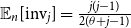 $\mathbb{E}_{n}[\textrm {inv}_{j}] =\frac {j(j-1)}{2(\theta + j - 1)}$
, which implies
 $\mathbb{E}_n[I_n] \sim n^2/4$
as we have seen. Similarly, we compute
 \begin{equation*} \mathbb{E}_{n}[\textrm {inv}_{j}^2] = \sum _{k=0}^{j-1}k^2\cdot {\mathbb{P}}_{n}(\textrm {inv}_{j}=k) = \sum _{k=1}^{j-1}k^2\cdot \frac {1}{\theta +j-1} = \frac {j(j-1)(2j-1)}{6(\theta + j - 1)}. \end{equation*}
Denoting
 ${\mathbb{V}}_n(\! \cdot \!)$
the variance of a random variable on record-biased permutations of size
 $n$
, it follows that
 \begin{equation*} {\mathbb{V}}_n(\textrm {inv}_j) = \frac {j(j-1)(2j-1)}{6(\theta + j - 1)} - \frac {j^2(j-1)^2}{4(\theta + j - 1)^2} = \frac {j(j-1)(j^2 +(4\theta -3)j +2-2\theta )}{12(\theta +j-1)^2}, \end{equation*}
so that
 ${\mathbb{V}}_n(I_n) \sim n^3/36$
as
 $n \to \infty$
.
Using Theorem 27.3 (p. 385) in [Reference Billingsley7] with the condition (27.16) for
 $\delta =1$
, to conclude the proof, it is enough to show that
 \begin{align*} \sum _{j=1}^n \frac {1}{\sqrt {\sum _{j=1}^n {\mathbb{V}}_n(\textrm {inv}_j)}^3} \mathbb{E}_n[\textrm {inv}_j^3] \to 0 \text{ as } n \to \infty . \end{align*}
With computations similar to those for
 $\mathbb{E}_n[\textrm {inv}_j]$
and
 $\mathbb{E}_n[\textrm {inv}_j^2]$
, we see that
 $\mathbb{E}_n[\textrm {inv}_j^3]$
is of order
 $j^3$
, so that
 $\sum _{j=1}^n \mathbb{E}_n[\textrm {inv}_j^3]$
is of order
 $n^4$
. On the other hand,
 $\sqrt {\sum _{j=1}^n {\mathbb{V}}_n(\textrm {inv}_j)}^3 = {\mathbb{V}}_n(I_n)^{3/2}$
is of order
 $n^{9/2}$
, and the proof is complete.
4.3.4 First value
Theorem 19.
Fix
 $\theta$
a positive real number. For
 $\sigma$
a record-biased permutation of size
 $n$
for the parameter
 $\theta$
, the random variable
 $\sigma (1)/n$
is asymptotically distributed following a beta distribution of parameters
 $(1,\theta )$
.
Proof. For any positive integer
 $r$
, the
 $r$
-th moment of a beta distribution of parameters
 $(1,\theta )$
is
 $\frac {r!}{(\theta +1)^{(r)}}$
(see e.g. [Reference Johnson, Kotz and Balakrishnan19, Ch. 25, p.217]). In particular, the associated moment generating function has positive radius of convergence, so that the beta distribution is determined by its moments (see e.g. [Reference Billingsley7, Thm 30.1]). Therefore, it is enough to compute the limits of the moments of
 $\sigma (1)/n$
, for
 $\sigma$
a record-biased permutation of size
 $n$
for the parameter
 $\theta$
, and to observe that these limits are indeed
 $\frac {r!}{(\theta +1)^{(r)}}$
.
To establish this, we use two properties of the Eulerian polynomials (which can be found e.g. in the recent book [Reference Petersen26, §1.4 and 1.5]). For any
 $r\gt 0$
, we denote by
 $A_r(z) = a_{r,0} + a_{r,1} z + \ldots + a_{r,r-1} z^{r-1}$
the Eulerian polynomial of degree
 $r-1$
. First,
 $a_{r,i}$
is the number of permutations of size
 $r$
with
 $i$
descents, so that we have
 $a_{r,0} + a_{r,1} + \ldots + a_{r,r-1} = r!$
. Second, the following identity (known as the Carlitz identity) holds, for any
 $r \gt 0$
:
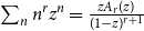 $\sum _n n^r z^n = \frac {z A_r(z)}{(1-z)^{r+1}}$
.
We can now proceed to the computation of the
 $r$
-th moment of
 $\sigma (1)$
, for
 $r\gt 0$
. (From the first to the second line, we use again the binomial formula as in the proof of Corollary13.)
 \begin{align*} \mathbb{E}_n[\sigma (1)^r] &= \sum _{k=1}^n k^r {\mathbb{P}}_{n}(\sigma (1)=k) = \frac {(n-1)!\theta }{\theta ^{(n)}} \sum _{k=1}^n k^r \frac {\theta ^{(n-k)}}{(n-k)!} = \frac {(n-1)!\theta }{\theta ^{(n)}} \sum _{j=0}^{n-1} (n-j)^r \frac {\theta ^{(j)}}{j!} \\[5pt] & = \frac {(n-1)!\theta }{\theta ^{(n)}} \sum _{j=0}^{n-1} [z^{n-j}] \frac {z A_r(z)}{(1-z)^{r+1}}\cdot [z^j] \frac {1}{(1-z)^\theta } \\[5pt] & = \frac {(n-1)!\theta }{\theta ^{(n)}} \sum _{j=0}^{n-1} [z^{n-j-1}] \frac {A_r(z)}{(1-z)^{r+1}}\cdot [z^j] \frac {1}{(1-z)^\theta } \\[5pt] & = \frac {(n-1)!\theta }{\theta ^{(n)}} [z^{n-1}] \frac {A_r(z)}{(1-z)^{r+1+\theta }} = \frac {(n-1)!\theta }{\theta ^{(n)}} [z^{n-1}] \frac {a_{r,0} + a_{r,1} z+ \ldots + a_{r,r-1} z^{r-1}}{(1-z)^{r+1+\theta }} \\[5pt] & = \frac {(n-1)!\theta }{\theta ^{(n)}} \sum _{j=1}^{r} a_{r,j-1} [z^{n-j}] \frac {1}{(1-z)^{r+1+\theta }} \end{align*}
Next, using the same trick once more, we compute (for
 $n$
large enough, namely
 $n-1 \geq r$
)
 \begin{align*} \frac {(n-1)!\theta }{\theta ^{(n)}} [z^{n-j}] \frac {1}{(1-z)^{r+1+\theta }} & = \frac {(n-1)!\theta }{\theta ^{(n)}} \frac {(\theta +r +1)^{(n-j)}}{(n-j)!} \\ & = \frac {(n-1) \ldots (n-j+1) \, \theta \, (\theta +r +1) \ldots (\theta +r+n-j)}{\theta (\theta +1) \ldots (\theta +n -1)} \\ & = \frac {(n-1) \ldots (n-j+1) \, (\theta +n) \ldots (\theta +r+n-j)}{(\theta +1) \ldots (\theta + r)} \\ & = \frac {n^{j-1} (1 + o(1)) \, n^{r-j+1} (1+o(1))}{(\theta +1)^{(r)}} = \frac {n^r (1+o(1))}{(\theta +1)^{(r)}}. \end{align*}
Finally,
 \begin{equation*} \mathbb{E}_n[\sigma (1)^r] = \sum _{j=1}^{r} a_{r,j-1} \frac {n^r (1+o(1))}{(\theta +1)^{(r)}} \text{ so that } \mathbb{E}_n[\sigma (1)^r] \sim _{n \to \infty } \frac {r! n^r}{(\theta +1)^{(r)}}. \end{equation*}
Therefore, dividing by
 $n^r$
, the
 $r$
-th moment of
 $\sigma (1)/n$
coincides with that of a beta distribution of parameters
 $(1,\theta )$
, concluding the proof.
Remark 20. We are aware of several alternative proofs of Theorem 19 that have been suggested by various colleagues.
First, up to a shift by
 $1$
, the first value of a permutation corresponds to the size of the right subtree at the root of its binary search tree (with the conventions of [Reference Corsini12] for building such trees). Theorem 19 therefore follows from the bounds of [Reference Corsini12, Lemma 2.4] and the subsequent remark; this remains valid provided that
 $\theta$
grows sub-linearly.
Second, using conditional expectation and computations similar to those in Remark 14, with the notation
 $Y_n$
from this remark, we can find a recurrence on
 $\mathbb{E}[Y_n(Y_n+1) \ldots (Y_n+r)]$
, for any integer
 $r \geq 0$
. This provides another way of computing the limiting behaviour of the
 $r$
-th moment of
 $\sigma (1)/n$
.
And third, from the probabilities of the elementary events obtained in Theorem 11, Stirling’s formula gives the asymptotic estimate
 ${\mathbb{P}}(Y_n = \lfloor yn\rfloor )\sim \frac {(1-y)^{\theta -1} \theta }{n}$
for any
 $y \in [0,1]$
. As
 $(1-y)^{\theta -1} \theta$
is the density of the beta distribution of parameters
 $(1,\theta )$
, Theorem 19 then follows from the so-called discrete Scheffé’s lemma, see e.g. [Reference Varin29, Corollary A.3].
5. Permuton limit
Using our efficient random samplers, we have been able to visualise diagrams of random record-biased permutations. This is how Figure 12 has been obtained. Explaining the limit shape that seems to emerge from this picture amounts to determining the permuton limit of random record-biased permutations. This is the purpose of this section.
Random permutations under the record-biased distribution on
 $\mathfrak{S}_{100}$
with, from left to right,
 $\theta =1$
(corresponding to the uniform distribution)
 $,50,100,$
and
 $500$
. For each diagram, the intensity of a point
 $(i,j)$
is proportional to the number of generated permutations
 $\sigma$
such that
 $\sigma (i)=j$
, for a sampling of 10000 random permutations of size
 $100$
.

Figure 12 Long description
The image contains four scatter plots side by side, each representing random permutations under different record-biased distributions on the symmetric group of degree 100. The x-axis ranges from 0 to 100, and the y-axis ranges from 0 to 100. Each plot shows the intensity of points (i, j) proportional to the number of generated permutations where σ(i) = j, based on a sampling of 10,000 random permutations of size 100. The leftmost plot corresponds to θ = 1, representing the uniform distribution, and shows a uniform spread of points. The subsequent plots, from left to right, correspond to θ = 50, 100, and 500, showing increasingly concentrated points along the diagonal as θ increases. The intensity of the points indicates the frequency of specific permutations, with darker regions representing higher frequencies. All values are approximated.
5.1 Permutons: definition and criterion of convergence
The notion of permutons was defined independently in [Reference Hoppen, Kohayakawa, Moreira, Rath and Sampaio18, Reference Presutti, Stromquist, Vatter, Linton and Ruškuc28], although the terminology was introduced later in [Reference Glebov, Grzesik, Klimošová and Král16]. It provides a convenient framework to describe the limits of permutations, once viewed as their rescaled diagrams – see e.g. [Reference Bassino, Bouvel, Féray, Gerin, Maazoun and Pierrot4, Reference Bassino, Bouvel, Féray, Gerin, Maazoun and Pierrot5, Reference Kenyon, Král, Radin and Winkler20].
Permutons, denoted
 $\mu$
here, are probability measures on the unit square
 $[0,1]^2$
such that
 \begin{equation} \text{for all } a \leq b \in [0,1], \quad \mu ([a,b]\times [0,1]) = b-a \text{ and } \mu ([0,1]\times [a,b]) = b-a. \end{equation}
Their projections on the horizontal and vertical axes are the uniform measure on
 $[0,1]$
. We sometimes say that permutons have uniform marginals because of the property of Eq. (5).
With every permutation
 $\sigma$
, denoting
 $n$
its size, we can associate a permuton as follows. Recall that the diagram of
 $\sigma$
consists of the set of points at coordinates
 $(i,\sigma (i))$
in an
 $n\times n$
grid. Rescaling the diagram to the unit square and replacing points by small squares carrying total mass
 $1$
, uniformly distributed, we obtain the permuton associated with
 $\sigma$
, which we denote
 $\mu _\sigma$
. See Figure 13. More formally,
 $\mu _\sigma$
is obtained dividing the unit square in a regular
 $n\times n$
grid and distributing uniformly the total mass
 $1$
on the small squares
 $[(i-1)/n,i/n]\times [(\sigma (i)-1)/n,\sigma (i)/n]$
. It is immediate to check that this construction ensures the uniform marginals property so that
 $\mu _\sigma$
is indeed a permuton for every permutation
 $\sigma$
.
The diagram and the permuton of
 $\sigma = 2 4 7 1 5 6 3$
.

Figure 13 Long description
A dot plot representing the permutation of sigma equals 2 4 7 1 5 6 3. The plot is a vertical grid with dots placed in specific cells. The x-axis represents the original position of elements, while the y-axis represents the permuted positions. Each dot indicates the position of an element in the permutation. The dots are scattered across the grid, showing the rearrangement of elements. The plot highlights the specific permutation pattern of the given sequence. All values are approximated.
Since permutons are measures, the weak convergence topology allows to define the notion of convergence of permutons. The distance between permutons is defined by
 \begin{equation} d_{all}(\mu , \nu ) = \sup (|\mu (R)-\nu (R)|), \end{equation}
where the supremum is taken over all rectangles
 $R = [a,b]\times [c, d]$
included in the unit square
 $[0,1]^2$
. Subsequently, a sequence
 $(\mu _n)_n$
of permutons converges to a permuton
 $\mu$
(which we write
 $\mu _n \to \mu$
) when
 $d_{all}(\mu _n,\mu ) \to 0$
. And for
 $(\mu _n)_n$
a sequence of random permutons,
 $\mu _n$
converges in probability to
 $\mu$
, which we write
 $\mu _n \xrightarrow {p} \mu$
, when for every
 $\varepsilon \gt 0$
it holds that
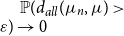 ${\mathbb{P}}(d_{all}(\mu _n,\mu )\gt \varepsilon ) \to 0$
as
 $n \to \infty$
.
We can define a variant
 $d(\mu , \nu )$
of the distance between permutons, similarly to Eq. (6), but where we take the supremum only over rectangles
 $R$
whose bottom-left corner is in
 $(0,0)$
. Although the distances differ, it is easy to see that they differ only by a factor of at most
 $4$
(this is also observed in [Reference Hoppen, Kohayakawa, Moreira, Rath and Sampaio18, eq. (34)]), so that
 $\mu _n \to \mu$
is equivalently defined by
 $d(\mu _n,\mu ) \to 0$
and
 $\mu _n \xrightarrow {p} \mu$
is equivalent to having, for every
 $\varepsilon \gt 0$
,
 ${\mathbb{P}}(d(\mu _n,\mu )\gt \varepsilon ) \to 0$
as
 $n \to \infty$
.
We will be particularly interested in the case where the converging sequence
 $\mu _n$
is random and obtained from a sequence of random permutations of increasing sizes, that is to say,
 $\mu _n$
is the random permuton associated with a random permutation
 $\sigma _n$
of size
 $n$
, for any
 $n$
. In this case, as the following lemma demonstrates, we can restrict even further the family of rectangles on which we take the supremum. Namely, we define
 \begin{equation*} d_{\cdot /n}(\mu , \nu ) = \sup (|\mu (R)-\nu (R)|), \end{equation*}
where
 $R$
ranges over the family
 $\mathcal{R}_n$
of rectangles of the form
 $[0,i/n]\times [0,j/n]$
, for
 $0\leq i,j \leq n$
.
Lemma 21.
For any
 $n$
, let
 $\sigma _n$
be a random permutation of size
 $n$
, and let
 $\mu _n$
be the associated random permuton. The following are equivalent:
-
•
$\mu _n \xrightarrow {p} \mu$
; -
• for every
$\varepsilon \in (0,1/2)$
, we have
${\mathbb{P}}(d_{\cdot /n} (\mu _n, \mu )\gt \varepsilon ) \to 0$
as
$n \to \infty$
.




In addition, if
 $(\sigma _n)_n$
is a sequence of (non-random) permutations with
 $|\sigma _n|=n$
and
 $\mu _n$
is the (non-random) associated permuton, we have equivalence between
 $\mu _n \to \mu$
and
 $d_{\cdot /n} (\mu _n,\mu ) \to 0$
as
 $n \to \infty$
.
Proof. For now, fix some positive integer
 $n$
. Let
 $R$
be any rectangle within
 $[0,1]^2$
whose bottom-left corner is in
 $(0,0)$
, and let
 $\nu$
be any permuton. We define
 $R^\square$
(resp.
 $R^\blacksquare$
) as the largest rectangle contained in
 $R$
(resp. smallest rectangle which contains
 $R$
) whose sides are supported by the lines of the regular
 $n\times n$
grid inside the unit square. In other words, we set
 \begin{equation*} R^\square =[0,a^\square ]\times [0,b^\square ] \text{ and } R^\blacksquare = [0,a^\square +\tfrac 1n]\times [0,b^\square +\tfrac 1n], \text{ for } a^\square = \tfrac 1n\lfloor an\rfloor \text{ and }b^\square = \tfrac 1n\lfloor bn\rfloor \end{equation*}
(unless
 $a^\square =a$
(resp.
 $b^\square =b$
), in which case we replace
 $a^\square +\tfrac 1n$
by
 $a^\square$
(resp.
 $b^\square +\tfrac 1n$
by
 $b^\square$
) in the definition of
 $R^\blacksquare$
).
Since
 $R^\square \subseteq R \subseteq R^\blacksquare$
, we have
 $\nu (R^\square )\leq \nu (R) \leq \nu (R^\blacksquare )$
. In addition,
 \begin{equation*} R^\blacksquare \subseteq R^\square \cup [a^\square ,a^\square +\tfrac 1n]\times [0,1] \cup [0,1]\times [b^\square ,b^\square +\tfrac 1n], \end{equation*}
so that
 $\nu (R^\blacksquare ) \leq \nu (R^\square ) + \frac 2n$
. In particular, it holds that
 $|\nu (R) - \nu (R^\square )| \leq \tfrac 2n$
. The second statement of Lemma21 then follows readily, since (with notation from this statement)
 \begin{equation*} d(\mu _n,\mu ) = \!\sup _{R = [0,a]\times [0,b]}\!(|\mu _n(R)-\mu (R)|) \leq \!\sup _{R = [0,a]\times [0,b]}\!(|\mu _n(R^\square )-\mu (R^\square )|+\tfrac 4n) = d_{\cdot /n}(\mu _n , \mu ) +\tfrac 4n. \end{equation*}
We now turn to the proof of the first statement (using notation from there), and more precisely to proving that the second item implies the first (the converse being obvious).
We first introduce notation. Recall that
 $\mathcal{R}_n$
is the set of rectangles of the form
 $[0,\tfrac {i}n]\times [0,\tfrac {j}n]$
for integers
 $i,j\leq n$
. For
 $\alpha \gt 0$
, let
 $\mathcal{M}^{\lt }_n(\alpha )$
and
 $\mathcal{M}^{\gt }_n(\alpha )$
be the following properties (recall that
 $\mu _n$
in the random permuton associated with the random permutation
 $\sigma _n$
of size
 $n$
):
 \begin{align*} \mathcal{M}^{\lt }_n(\alpha ) & = \exists R^\square \in \mathcal{R}_n,\ \mu _n(R^\square ) \lt \mu (R^\square ) -\alpha \\ \mathcal{M}^{\gt }_n(\alpha ) & = \exists R^\square \in \mathcal{R}_n,\ \mu _n(R^\square ) \gt \mu (R^\square ) + \alpha . \end{align*}
Under the assumption of the second item, for any fixed
 $\alpha \gt 0$
, the properties
 $\mathcal{M}^{\lt }_n(\alpha )$
and
 $\mathcal{M}^{\gt }_n(\alpha )$
both have a probability tending to
 $0$
as
 $n$
tends to
 $\infty$
. Also note that, for any
 $\beta \leq \alpha$
,
 $\mathcal{M}^{\lt }_n(\alpha )$
implies
 $\mathcal{M}^{\lt }_n(\beta )$
, hence
 ${\mathbb{P}}(\mathcal{M}^{\lt }_n(\alpha )) \leq {\mathbb{P}}(\mathcal{M}^{\lt }_n(\beta ))$
, and similarly with
 $\mathcal{M}^{\gt }_n$
.
Fix some
 $\varepsilon \in (0,1/2)$
. We first observe (using the union bound) that
 \begin{multline*} {\mathbb{P}}\left (\sup _{R = [0,a]\times [0,b]}\left | \mu _n(R)-\mu (R)\right |\gt \varepsilon \right ) = {\mathbb{P}}\left (\exists R = [0,a]\times [0,b],\ |\mu _n(R) - \mu (R)| \gt \varepsilon \right ) \\ \leq {\mathbb{P}}\left (\exists R = [0,a]\times [0,b],\ \mu _n(R) - \mu (R) \gt \varepsilon \right ) + {\mathbb{P}}\left (\exists R = [0,a]\times [0,b],\ \mu (R) - \mu _n(R) \gt \varepsilon \right ). \end{multline*}
Next, from the inequalities established above, assuming that
 $\mu _n(R) \gt \mu (R) + \varepsilon$
, we have
 \begin{equation*} \mu _n(R^\square ) +\tfrac 2n \geq \mu _n(R) \gt \mu (R) + \varepsilon \geq \mu (R^\square ) + \varepsilon , \text{ hence } \mu _n(R^\square ) \gt \mu (R^\square ) + \varepsilon -\tfrac 2n. \end{equation*}
Similarly, if
 $\mu (R) - \mu _n(R) \gt \varepsilon$
, then
 $\mu _n(R^\square ) \lt \mu (R^\square ) - \varepsilon +\tfrac 2n$
. As a consequence,
 \begin{equation*} {\mathbb{P}}\left (\sup _{R = [0,a]\times [0,b]}\left | \mu _n(R)-\mu (R)\right |\gt \varepsilon \right ) \leq {\mathbb{P}}\big (\mathcal{M}^{\gt }_n \big(\varepsilon -\tfrac 2n\big)\big ) + {\mathbb{P}}\big(\mathcal{M}^{\lt }_n\big(\varepsilon -\tfrac 2n\big)\big ). \end{equation*}
Therefore, for
 $n$
large enough (i.e., such that
 $\tfrac {\varepsilon }2 \lt \varepsilon -\tfrac 2n$
),
 \begin{equation*} {\mathbb{P}}\left (\sup _{R = [0,a]\times [0,b]}\left | \mu _n(R)-\mu (R)\right |\gt \varepsilon \right ) \leq {\mathbb{P}}\big(\mathcal{M}^{\gt }_n\big(\tfrac {\varepsilon }2\big)\big ) + {\mathbb{P}}\big (\mathcal{M}^{\lt }_n\big(\tfrac {\varepsilon }2 \big)\big ), \end{equation*}
ensuring that
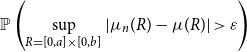 ${\mathbb{P}}\left (\sup \limits _{R = [0,a]\times [0,b]}\left | \mu _n(R)-\mu (R)\right |\gt \varepsilon \right )$
tends to
 $0$
as
 $n$
tends to
 $\infty$
.
Finally, we point out an important result about permuton convergence: it is equivalent to the convergence of all pattern densities – see [Reference Hoppen, Kohayakawa, Moreira, Rath and Sampaio18, Reference Presutti, Stromquist, Vatter, Linton and Ruškuc28] in the deterministic case, or [Reference Bassino, Bouvel, Féray, Gerin, Maazoun and Pierrot4, §2] for convergence of sequences of random permutons. In the present work, we do not use this characterisation and refer the interested reader to the above papers for details.
5.2 The permuton limit of record-biased permutations for
$\theta = \lambda n$

In this section, we define a permuton
 $\mu$
, which we later prove (see Theorem25 and Subsection 5.4) to be the limit of the sequence of random permutations
 $(\sigma _n)_n$
defined as follows: for each
 $n$
,
 $\sigma _n$
is a random record-biased permutation of size
 $n$
, for the parameter
 $\theta = \lambda n$
. (The reader may notice that this is a different regime than the main one studied in Section 4, where
 $\theta$
was taken as a fixed positive real number.)
Let
 $\lambda \gt 0$
be a parameter. Let
 $f_\lambda \, : \, [0,1] \to [0,1]$
be the function defined by
 $f_\lambda (x) = \frac {x(\lambda +1)}{\lambda +x}$
. It is obvious but useful to observe that
 $f_\lambda$
is continuous and increasing from
 $f_\lambda (0)=0$
to
 $f_\lambda (1)=1$
. It is therefore invertible, and its inverse is given by
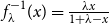 $f_\lambda ^{-1}(x) =\frac {\lambda x}{1+\lambda -x}$
. Similarly, an obvious but useful fact is that
 $f_\lambda (x) \geq x$
for all
 $x \in [0,1]$
.
We define
 $Leb_c$
as the measure on the unit square whose support is the curve of equation
 $y = f_\lambda (x)$
, with the mass
 $1$
distributed uniformly along the
 $x$
-axis: in other words, for all
 $a$
,
 $Leb_c(\{(x,f_\lambda (x))\, : \, x \in [0,a]\})$
has measure
 $a$
. Then, we define
 $\mu _c$
as the measure with density
 $\frac {\lambda }{\lambda +x}$
with respect to
 $Leb_c$
.
We also define
 $\mu _u$
as the measure on the unit square whose support is the area below the curve of equation
 $y = f_\lambda (x)$
, and with mass
 $\frac {1}{\lambda +1} \int _0^1 f_\lambda (x)dx$
uniformly distributed on this support.
Finally, we let
 $\mu = \mu _c + \mu _u$
(examples are displayed in Figure 14).
From left to right: graphical representation of
 $\mu$
for
 $\lambda =0.05$
,
 $0.2$
and
 $1$
.

Figure 14 Long description
The image contains three line graphs side by side, each representing the graphical representation of the Greek letter mu for different values of lambda. The graphs from left to right correspond to lambda values of 0.05, 0.2, and 1. Each graph shows a curve that starts steeply and gradually flattens out as it moves to the right. The x-axis and y-axis are not labeled, but the curves illustrate how the value of mu changes with respect to lambda. All values are approximated.
Remark 22. We mention that the article [Reference Alon, Defant and Kravitz1] defines another permuton (called the runsort permuton) as the sum of a singular part supported by a curve and an absolutely continuous part supported by the part of the unit square above this curve. Our permuton
 $\mu$
(up to symmetry) and the runsort permuton therefore share a qualitatively similar behaviour.
Lemma 23.
The measure
 $\mu$
on the unit square defined above is a permuton.
Proof. We claim that, for each
 $0\leq a\leq b \leq 1$
,
 $\mu ([a,b]\times [0,1]) =b-a$
. This ensures (for
 $a=0,b=1$
) that
 $\mu$
is a probability measure on the unit square; and it also ensures one part of the uniform marginals property. This claim is easily proved; indeed, we have
 \begin{align*} \mu ([a,b]\times [0,1]) &= \int _a^b \frac {\lambda }{\lambda +x} dx + \frac {1}{\lambda +1} \int _a^b f_\lambda (x)dx = \int _a^b \left (\frac {\lambda }{\lambda +x} +\frac {f_\lambda (x)}{\lambda +1}\right ) dx\\ & = \int _a^b \left (\frac {\lambda }{\lambda +x} +\frac {x}{\lambda +x}\right ) dx \quad \text{substituting}\,\, f_\lambda (x)\, \text{by its definition} \\ & = b-a. \end{align*}
It remains to show that for each
 $0\leq a\leq b \leq 1$
,
 $\mu ([0,1]\times [a,b]) =b-a$
. For this, we prove below that
 $\mu ([0,1]\times [a,b]) = \mu ([1-b,1-a]\times [0,1])$
. From there, we can use the above computation to derive
 $\mu ([1-b,1-a]\times [0,1])= (1-a) - (1-b) = b-a$
.
To prove
 $\mu ([0,1]\times [a,b]) = \mu ([1-b,1-a]\times [0,1])$
, we shall prove that this identity holds for
 $\mu _u$
and for
 $\mu _c$
, and then deduce it for
 $\mu = \mu _u + \mu _c$
.
We first observe that the curve of equation
 $y=f_\lambda (x)$
is symmetric along the line of equation
 $y=1-x$
(the NorthWest-SouthEast diagonal of the unit square): this follows from the equality
 $f_\lambda (1-f_\lambda (x)) = 1-x$
, which is just proved by a simple computation. And this is enough to ensure that
 $\mu _u([0,1]\times [a,b]) = \mu _u([1-b,1-a]\times [0,1])$
.
Now, recalling that
 $\mu _c$
is the measure with density
 $\frac {\lambda }{\lambda +x}$
with respect to
 $Leb_c$
, we have
 \begin{align*} \mu _c([1-b,1-a]\times [0,1]) & = \int _{1-b}^{1-a} \frac {\lambda }{\lambda +x} dx = \left [ \lambda \log (\lambda +x)\right ]_{1-b}^{1-a} = \lambda \log \left (\frac {\lambda +1-a}{\lambda +1-b}\right )\!, \text{ and}\\ \mu _c([0,1]\times [a,b]) & = \int _{f_\lambda ^{-1}(a)}^{f_\lambda ^{-1}(b)} \frac {\lambda }{\lambda +x} dx = \left [ \lambda \log (\lambda +x)\right ]_{f_\lambda ^{-1}(a)}^{f_\lambda ^{-1}(b)} = \lambda \log \left (\frac {\lambda +1-a}{\lambda +1-b}\right ) \!, \end{align*}
where we used that the inverse of
 $f_\lambda$
is given by
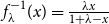 $f_\lambda ^{-1}(x) =\frac {\lambda x}{1+\lambda -x}$
. This ensures, as wanted, that
 $\mu _c([0,1]\times [a,b]) = \mu _c([1-b,1-a]\times [0,1])$
and therefore concludes the proof.
Remark 24. We point out that the permuton
 $\mu$
(or rather its symmetry w.r.t. a horizontal axis, which we denote
 $\mu ^R$
below) appeared in a similar context in the PhD thesis of J. Borga [Reference Borga9, Ch. 5], however in disguise.
We first explain how to regonise
 $\mu ^R$
in [Reference Borga9, §5.2.3]. By symmetry, from our definition of
 $\mu$
, the permuton
 $\mu ^R$
consists of two parts:
-
• a first part supported by the curve of equation
$y = 1-f_\lambda (x) = 1- \frac {x(\lambda +1)}{\lambda +x}$
, of total mass
$\int _a^b \frac {\lambda }{\lambda +x} dx = \lambda \log (1+1/\lambda )$
; -
• and a second part, above this curve, where the mass
$ \frac {1}{\lambda +1} \int _0^1 f_\lambda (x)dx = 1 - \lambda \log (1+1/\lambda )$
is uniformly distributed.



On the other hand, the permuton
 $\nu$
defined in [Reference Borga9, §5.2.3] (where it is denoted
 $\nu ^\alpha _*$
) is described as follows. Given a positive
 $\alpha$
, let
 $\gamma$
be the solution of
 $\tfrac {1}{\gamma -1}\log (\gamma ) = \tfrac {1}{\alpha +1}$
. Then
 $\nu$
consists of two parts:
-
• a first part supported by the curve parametrised by
$(\tfrac {\gamma ^t-1}{\gamma -1},\tfrac {\gamma ^{1-t}-1}{\gamma -1})$
for
$t \in [0,1]$
, of total mass
$\tfrac {1}{\alpha +1}$
; -
• and a second part, above this curve, where the mass
$\tfrac {\alpha }{\alpha +1}$
is uniformly distributed.


It is straightforward to check that
 $\mu ^R = \nu$
, if we take
 $\alpha = \tfrac {1}{\lambda \log (1+1/\lambda )} -1$
, or equivalently
 $\lambda =\tfrac {1}{\gamma -1}$
.
We now describe the context in which
 $\nu$
appeared in [Reference Borga9, Ch. 5]. Specifically, Conjecture 5.2.6 in [Reference Borga9] states that
 $\nu = \mu ^R$
is the permuton limit of uniform permutations of size
 $m=n+k$
with exactly
 $n$
left-to-right minima and
 $k$
elements which are not left-to-right minima, with
 $n$
and
 $k$
both tending to
 $\infty$
with
 $k/n \to \alpha$
for some positive
 $\alpha$
. This is equivalent to stating that
 $\mu$
is the permuton limit of uniform permutations of size
 $m=n+k$
with exactly
 $n$
records and
 $k$
non-records, in the same regime for
 $n$
and
 $k$
.
While this is different from our model of record-biased permutations, we note that the number of records in the model of [Reference Borga9] is in the limit
 $\frac {1}{\alpha +1}$
times the total size of the permutation. In our model, we have seen (see Table 1) that the number of records is in the limit
 $\lambda \log (1+1/\lambda )$
times the total size. We observe that, with the relation
 $\alpha = \tfrac {1}{\lambda \log (1+1/\lambda )} -1$
given earlier,
 $\frac {1}{\alpha +1} = \lambda \log (1+1/\lambda )$
. It may therefore be possible that an improvement of Theorem25 (establishing the convergence of
 $\mu _n$
to
 $\mu$
) with an additional concentration result could be used to prove Conjecture 5.2.6 in [Reference Borga9].
5.3 On guessing the candidate limit
$\mu$

Our proof of the convergence of
 $\mu _n$
to
 $\mu$
in Subsection 5.4 provides no information on why
 $\mu$
has been defined as it is. The purpose of this section is therefore to explain how we identified the candidate limit
 $\mu$
. We emphasie that this is not necessary for the proof to come and included only so that readers can understand why
 $\mu$
is the natural candidate for the limit and how we found it.
All along this section, we fix a value
 $\lambda \gt 0$
, and for each
 $n$
, we let
 $\sigma _n$
denote a random record-biased permutation of size
 $n$
, for the parameter
 $\theta = \lambda n$
.
5.3.1 Equation of the curve
The curve of equation
 $y=f_\lambda (x)$
is, informally speaking, describing the limit of the broken lines which interpolate between the records of
 $\sigma _n$
. We start by presenting how the expression of
 $f_\lambda$
was derived.
For
 $\sigma$
a permutation of size
 $n$
and
 $i\in [n]$
, let
 $\textrm {lmax}(\sigma ,i)=\max \{\sigma (j) \, : \, j\in [i]\}$
be the last (and largest) record occurring at or before position
 $i$
. We are interested in
 ${\mathbb{P}}(\textrm {lmax}(\sigma _n,i)=j)$
for
 $i\approx xn$
and
 $j\approx yn$
, and
 $x,y\in (0,1)$
. The idea is that the equation of the curve is obtained by finding the value
 $y$
that maximises this probability for any given
 $x\in (0,1)$
.
To compute this probability, we decompose permutations of size
 $n$
, and we examine the contribution of each part of this decomposition to their weight in the record-biased distribution.
A permutation
 $\sigma$
of size
 $n$
such that
 $\textrm {lmax}(\sigma ,i)=j$
is decomposed as follows.
-
• First, observe that necessarily
$j\geq i$
. So, we first choose the images by
$\sigma$
of
$[i]$
in
$[j]$
(there are
$\binom {j-1}{i-1}$
possibilities, as
$j$
belongs to this set). Once chosen, permuting them in all possible ways yields a total contribution to the weight of
$\theta ^{( i)}$
. -
• Then we identify the positions of the
$j-i$
remaining images that are smaller than
$j$
, all occurring after position
$i$
. There are
$\binom {n-i}{j-i}$
possible sets of preimages for them, and
$(j-i)!$
ways to assign them; as none of these elements are records, the total weight remains unchanged. -
• The remaining images (all those of value greater than
$j$
) are assigned to the remaining positions, in any possible fashion. The total weight on all possible permutations of these remaining images is
$\theta ^{( {n-j})}$
.


Therefore, we have, for
 $j\geq i$
,
 \begin{equation} {\mathbb{P}}(\textrm {lmax}(\sigma _n, i)=j) = \frac {{\theta ^{(i )}}{\theta ^{(n-j)}}}{\theta ^{(n )}}\binom {j-1}{i-1} \binom {n-i}{j-i}(j-i)! = \frac {{\theta ^{( i)}}{\theta ^{(n-j)}}}{\theta ^{( n)}}\frac {i}{j}\binom {j}{i} \binom {n-i}{j-i}(j-i)!. \end{equation}
Now we proceed informally by using
 $i=xn$
,
 $j=yn$
(recall also that
 $\theta = \lambda n$
). We want to establish asymptotic estimates for all the factors occurring in the above expression of
 ${\mathbb{P}}(\textrm {lmax}(\sigma _n, i)=j)$
. First,
 \begin{equation*} {\theta ^{( i)}} =\frac {\Gamma (\lambda n+xn)}{\Gamma (\lambda n)} =\frac {\lambda n}{(\lambda +x)n}\frac {\Gamma (\lambda n+xn+1)}{\Gamma (\lambda n+1)} \sim \sqrt {\frac {\lambda }{\lambda +x}} \left (\frac {(\lambda +x)^{\lambda +x}}{\lambda ^{\lambda }}\right )^{n} n^{xn} e^{-xn} \end{equation*}
Similarly, we find
 \begin{align*} {\theta ^{(n )}{}} & \sim \sqrt {\frac {\lambda }{\lambda +1}} \left (\frac {(\lambda +1)^{\lambda +1}}{\lambda ^{\lambda }}\right )^{n} n^{n} e^{-n} \text{ and}\\ {\theta ^{({n-j} )}} & \sim \sqrt {\frac {\lambda }{\lambda +1-y}} \left (\frac {(\lambda +1-y)^{\lambda +1-y}}{\lambda ^{\lambda }}\right )^{n} n^{(1-y)n} e^{-(1-y)n}. \end{align*}
Hence
 \begin{equation*} \frac {{\theta ^{( i)}}{\theta ^{(n-j)}}}{\theta ^{(n)}} \sim {\sqrt {\frac {\lambda (\lambda +1)}{(\lambda +x)(\lambda +1-y)}}} \left (\frac {(\lambda +x)^{\lambda +x}(\lambda +1-y)^{\lambda +1-y}}{\lambda ^{\lambda }(\lambda +1)^{\lambda +1}}\right )^{n} n^{(x-y)n}e^{-(x-y)n}.\end{equation*}
For the factors which do not involve
 $\theta$
, we have
 \begin{equation*} \binom {n-i}{j-i}(j-i)! = \frac {\Gamma (n-i+1)}{\Gamma (n-j+1)} \sim \sqrt {\frac {1-x}{1-y}} \left (\frac {(1-x)^{1-x}}{(1-y)^{1-y}}\right )^{n}e^{(x-y)n}n^{-(x-y)n}, \end{equation*}
and
 \begin{equation*} \frac {i}{j}\binom {j}{i} \sim \frac 1{\sqrt {2\pi n}} \frac {x}{y} \sqrt {\frac {y}{x(y-x)}} \left (\frac {y^{y}}{x^{x}(y-x)^{y-x}}\right )^{n}. \end{equation*}
Putting everything together, we obtain
 \begin{equation} {\mathbb{P}}(\textrm {lmax}(\sigma _n, i)=j) \sim \frac 1{\sqrt {2\pi n}} \sqrt {\frac {x(1-x){\lambda (\lambda +1)}}{y(1-y)(y-x){(\lambda +x)(\lambda +1-y)}}} F(x,y)^{n}, \end{equation}
with
 \begin{equation} F(x,y) = \frac {y^{y}(1-x)^{1-x}(\lambda +x)^{\lambda +x}(\lambda +1-y)^{\lambda +1-y}}{x^{x}(y-x)^{y-x}(1-y)^{1-y}\lambda ^{\lambda }(\lambda +1)^{\lambda +1}}. \end{equation}
It is necessary that
 $F(x,y)\leq 1$
, otherwise the probability would be greater than
 $1$
for
 $n$
sufficiently large. Even more, for any given
 $x$
, we claim that there is at least one
 $y$
such that
 $F(x,y)=1$
. Indeed, assuming otherwise, by continuity of
 $F$
we can make
 $\sum _{j}{\mathbb{P}}(\textrm {lmax}(\sigma _n, i)=j)$
as small as we want, which is not possible as it is equal to
 $1$
.
Therefore, the equation of the curve we are looking for is given by finding, for each
 $x$
, the value of
 $y$
such that
 $F(x,y) = 1$
, i.e. which maximises
 $F(x,y)$
. Rather than solving
 $F(x,y) = 1$
or
 $\frac {d}{dy}F(x,y) = 0$
, we can solve
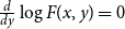 $\frac {d}{dy}\log F(x,y) = 0$
, for which computations are easier, since
 \begin{equation*} \frac {d}{dy}\log F(x,y) = \log \left (\frac {y(1-y)}{(y-x)(\lambda +1-y)}\right ) \!. \end{equation*}
Hence
 \begin{equation*} \frac {d}{dy}\log F(x,y) = 0 \Leftrightarrow y = \frac {x(\lambda +1)}{\lambda +x}, \end{equation*}
which justifies our definition of the function
 $f_\lambda (x) = \frac {x(\lambda +1)}{\lambda +x}$
in the previous section.
By contruction, it holds that
 \begin{equation} \text{for all $x$, } F(x,f_\lambda (x))=1. \end{equation}
It is also possible to check (e.g. in Maple) from the explicit expression of
 $F(x,y)$
and of
 $f_\lambda (x)$
that the equality
 $F(x,f_\lambda (x))=1$
indeed holds for all
 $x$
.
5.3.2 Density on the curve
Next, we want to determine the density of the measure
 $\mu _c$
whose support is the curve of equation
 $y = f_\lambda (x)$
. Informally, the total mass on this curve is the limit of the measure carried by all the records in the permutation
 $\sigma _n$
. To compute it, let us first recall that, in a permutation of size
 $n$
,
 $\frac {1}{n}$
is the measure associated with every point of
 $\sigma$
(to ensure that the total measure of all points is
 $1$
). So, using Theorem1, we obtain that the total measure carried by all the records in
 $\sigma _n$
is
 \begin{equation*} \sum _{i=1}^n \frac {1}{n} {\mathbb{P}}_{n}(\text{record at }i) = \frac {1}{n} \sum _{i=1}^n \frac {\theta }{\theta + i - 1} = \frac {1}{n} \sum _{i=1}^n \frac {\lambda }{\lambda + i/n - 1/n}. \end{equation*}
Up to the
 $1/n$
(that we neglect), this is a Riemann sum, and taking
 $n \to \infty$
, the limit is
 $ \int _0^1 \frac {\lambda }{\lambda +x} dx.$
If we were considering only records occurring between position
 $i \approx an$
and
 $j \approx bn$
, the measure carried by these records would similarly be
 $ \int _a^b \frac {\lambda }{\lambda +x} dx.$
This explains how the density
 $\frac {\lambda }{\lambda +x}$
of the measure
 $\mu _c$
was determined.
5.3.3 Density below the curve
Finally, we need to “complete”
 $\mu _c$
by a measure
 $\mu _u$
under the curve of equation
 $y=f_\lambda (x)$
in such a way that we obtain a permuton. In particular, we must ensure the uniform marginals property.
By definition,
 \begin{equation*} \mu _c([a,b]\times [0,1]) = \int _a^b \frac {\lambda }{\lambda +x} dx. \end{equation*}
Therefore, if we want to put a uniform measure of area density
 $a_\lambda$
under the curve, it needs to satisfy
 \begin{equation*} \text{for all } a \lt b \in [0,1], \int _a^b \left ( \frac {\lambda }{\lambda +x} + a_\lambda f_\lambda (x) \right ) dx = b-a. \end{equation*}
Recalling that
 $f_\lambda (x) = \frac {x(\lambda +1)}{\lambda +x}$
, the condition above is satisfied when taking
 $a_{\lambda }=\frac {1}{\lambda +1}$
.
5.4 Proof of the permuton limit
Throughout this section, we fix
 $\lambda \gt 0$
. Recall that, for each integer
 $n$
,
 $\sigma _n$
denotes a random record-biased permutation of size
 $n$
, for the parameter
 $\theta = \lambda n$
. Recall also that for
 $i\in [n]$
,
 $\textrm {lmax}(\sigma _n,i)=\max \{\sigma (j)\, : \, j\in [i]\}$
denotes the last (and largest) record occurring at or before position
 $i$
. Finally, recall that
 $\mu _n$
is the (random) permuton associated with
 $\sigma _n$
, and that the permuton
 $\mu$
has been defined in Subsection 5.2.
The rest of the paper is devoted to proving our main result in this section.
Theorem 25.
It holds that
 $\mu _n$
converges in probability to
 $\mu$
(w.r.t. the weak topology).
The first step of our proof is to show that
 $\textrm {lmax}(\sigma _n,i)$
is concentrated around its typical value. This appears below as Proposition 26.
Proposition 26. For every
 $\varepsilon \gt 0$
, there exists
 $c(\varepsilon ) \in (0,1)$
such that for
 $n$
sufficiently large we have:
 \begin{equation*} \text{for all } i \in \{1,\ldots ,n\} \text{ such that } \varepsilon \lt f_\lambda (i/n) \lt 1-\varepsilon , \ \mathbb{P}\left (|{\operatorname{lmax}}(\sigma _n,i) - nf_\lambda (i/n)|\gt \varepsilon \,n\right ) \leq c(\varepsilon )^n. \end{equation*}
Establishing this result essentially consists in transforming the estimate in Eq. (8) – which is only informal (and qualitative) – into a precise (and quantitative) statement. To this effect, we shall need tight upper and lower bounds on the rising factorials (Lemma27). We then use them to establish upper and lower bounds on
 ${\mathbb{P}}(\textrm {lmax}(\sigma _n, i)=j)$
(Lemma28). Both bounds are of the same order as the estimate in Eq. (8) up to polynomial factors.
Lemma 27.
For any positive integer
 $n$
and any real
 $\alpha {\in [0,1]}$
such that
 $\alpha n$
is an integer, we have
 \begin{equation*} \frac 1{{c_\lambda ^2}}\left (\frac {(\lambda +\alpha )^{\lambda +\alpha }}{\lambda ^\lambda e^{\alpha }}\right )^n\,n^{\alpha n} \leq (\lambda n)^{(\alpha n)} \leq c_\lambda \left (\frac {(\lambda +\alpha )^{\lambda +\alpha }}{\lambda ^\lambda e^{\alpha }}\right )^n\,n^{\alpha n}, \text{ with }c_\lambda = \sqrt {\frac {\lambda +1}\lambda }. \end{equation*}
Proof. We use the fact that for all
 $x\gt 0$
, we have [Reference Batir6, Thm 1.6]
 \begin{equation} x^x e^{-x} \sqrt {2\pi x} \leq \Gamma (x+1)\leq x^x e^{-x} \sqrt {2\pi (x+1)}. \end{equation}
As
 $\theta ^{(i)}=\frac {\Gamma (\theta +i)}{\Gamma (\theta )}= \frac {\theta }{\theta +i} \frac {\Gamma (\theta +i+1)}{\Gamma (\theta +1)}$
we have, for
 $n\geq 1$
 \begin{align*} (\lambda n)^{(\alpha n)} & \leq \frac {\lambda n}{\lambda n + \alpha n} \frac {((\lambda n +\alpha n)e^{-1})^{\lambda n+\alpha n} \sqrt {2\pi (\lambda n+\alpha n +1)}}{((\lambda n)e^{-1})^{\lambda n}\sqrt {2\pi \lambda n}}\\ &\leq \frac {\lambda }{\lambda + \alpha } \left (\frac {(\lambda +\alpha )^{\lambda +\alpha }}{\lambda ^\lambda e^{\alpha }}\right )^n \frac {\sqrt {(\lambda +\alpha +1)}}{\sqrt {\lambda }}\,n^{\alpha n}\\ & \leq d_\lambda \left (\frac {(\lambda +\alpha )^{\lambda +\alpha }}{\lambda ^\lambda e^{\alpha }}\right )^n\,n^{\alpha n}, \end{align*}
where
 $d_\lambda = \max _{\alpha {\in [0,1]}}\frac {\sqrt {\lambda (\lambda +\alpha +1)}}{\lambda +\alpha } = \sqrt {\frac {\lambda +1}\lambda }.$
The lower bound works similarly:
 \begin{align*} (\lambda n)^{(\alpha n)} & \geq \frac {\lambda n}{\lambda n + \alpha n} \frac {((\lambda n +\alpha n)e^{-1})^{\lambda n+\alpha n} \sqrt {2\pi (\lambda n+\alpha n)}}{((\lambda n)e^{-1})^{\lambda n}\sqrt {2\pi (\lambda n+1)}}\\ &\geq \frac {\lambda }{\lambda + \alpha } \left (\frac {(\lambda +\alpha )^{\lambda +\alpha }}{\lambda ^\lambda e^{\alpha }}\right )^n \frac {\sqrt {\lambda +\alpha }}{\sqrt {\lambda +1}}\,n^{\alpha n}\\ & \geq e_\lambda \left (\frac {(\lambda +\alpha )^{\lambda +\alpha }}{\lambda ^\lambda e^{\alpha }}\right )^n\,n^{\alpha n}, \end{align*}
where
 $e_\lambda = \min _{\alpha {\in [0,1]}}\frac {\lambda }{\sqrt {\lambda +1}}\cdot \frac 1{\sqrt {\lambda +\alpha }} = {\frac {\lambda }{\lambda +1}}$
. This concludes the proof.
Recall from Eq. (9) that
 $F(x,y) = \frac {y^{y}(1-x)^{1-x}(\lambda +x)^{\lambda +x}(\lambda +1-y)^{\lambda +1-y}}{x^{x}(y-x)^{y-x}(1-y)^{1-y}\lambda ^{\lambda }(\lambda +1)^{\lambda +1}}$
.
Lemma 28.
For
 $n$
sufficiently large, and for all
 $1\lt i\leq j\leq n-1$
, it holds that
 \begin{equation*} n^{-5} \cdot F \left(\tfrac {i}n,\tfrac {j}n\right)^n\leq \mathbb{P}({\mathrm {lmax}}(\sigma _n,i)=j) \leq n^3 \cdot F\left(\tfrac {i}n,\tfrac {j}n\right)^n.\end{equation*}
Note that only the upper bound in the above proposition is needed later. However, obtaining the lower bound does not require much more work, so we record it here for completeness.
Proof. Let
 $j$
be an integer such that
 $i\leq j \lt n$
. From Eq. (7), we have
 \begin{equation*} \mathbb{P}(\textrm {lmax}(\sigma _n,i)=j) = \frac {i}{j}\frac {\theta ^{(i)}\theta ^{(n-j)}}{\theta ^{(n)}}\binom {j}{i}\binom {n-i}{j-i}(j-i)!. \end{equation*}
Let
 $\alpha = i/ n$
and
 $\beta =j/n$
(noting that this implies
 $\alpha \leq \beta$
). From Lemma27, we have
 \begin{align*} \frac {\theta ^{(i)}\theta ^{(n-j)}}{\theta ^{(n)}} & \leq c_\lambda ^3 \left (\frac {(\lambda +\alpha )^{\lambda +\alpha }}{\lambda ^\lambda e^\alpha }\right )^n \left (\frac {(\lambda +1-\beta )^{\lambda +1-\beta }}{\lambda ^\lambda e^{1-\beta }}\right )^n \left (\frac {(\lambda +1)^{\lambda +1}}{\lambda ^\lambda e}\right )^{-n} n^{(\alpha -\beta )n}\\ &\leq c^3_\lambda \left (\frac {(\lambda +\alpha )^{\lambda +\alpha }(\lambda +1-\beta )^{\lambda +1-\beta }}{\lambda ^\lambda (\lambda +1)^{\lambda +1} e^{\alpha -\beta }}\right )^n n^{(\alpha -\beta )n}. \end{align*}
And similarly,
 \begin{align*} \frac {\theta ^{(i)}\theta ^{(n-j)}}{\theta ^{(n)}} & \geq \frac 1{{c^6_\lambda }} \left (\frac {(\lambda +\alpha )^{\lambda +\alpha }(\lambda +1-\beta )^{\lambda +1-\beta }}{\lambda ^\lambda (\lambda +1)^{\lambda +1} e^{\alpha -\beta }}\right )^n n^{(\alpha -\beta )n}. \end{align*}
We now use the following (crude) Stirling bounds:
 \begin{equation} \forall n\geq 0,\ n^{n}e^{-n} \leq n!\quad \text{and}\quad \forall n\geq 1,\ n! \leq 3n^{n+1}e^{-n}. \end{equation}
Hence
 \begin{equation*} \binom {j}{i} = \frac {j!}{i!(j-i)!} \leq \frac {3j^{j+1}}{e^j}\frac {e^i}{i^i}\frac {e^{j-i}}{(j-i)^{j-i}} \leq 3n \left (\frac {\beta ^\beta }{\alpha ^\alpha (\beta -\alpha )^{\beta -\alpha }}\right )^n, \end{equation*}
and
 \begin{equation*} \binom {n-i}{j-i} (j-i)! = \frac {(n-i)!}{(n-j)!} \leq \frac {3(n-i)^{n-i+1}}{e^{n-i}} \frac {e^{n-j}}{(n-j)^{n-j}} \leq 3n \left (e^{\alpha -\beta } \frac {(1-\alpha )^{1-\alpha }}{(1-\beta )^{1-\beta }} \right )^n n^{(\beta -\alpha )n}. \end{equation*}
Putting all together, we get
 \begin{align*} \mathbb{P}(\textrm {lmax}(\sigma _n,i)=j) & \leq 9n^2 c_\lambda ^3 \frac {\alpha }{\beta }\left [\frac {(\lambda {+}\alpha )^{\lambda {+}\alpha }(\lambda +1-\beta )^{\lambda {+}1{-}\beta }}{\lambda ^\lambda (\lambda +1)^{\lambda {+}1}}\right ]^n \left (\frac {\beta ^\beta }{\alpha ^\alpha (\beta {-}\alpha )^{\beta {-}\alpha }}\right )^n\left ( \frac {(1{-}\alpha )^{1{-}\alpha }}{(1-\beta )^{1{-}\beta }} \right )^n \\ & \leq 9n^2 c_\lambda ^3 \frac {\alpha }{\beta } F(\alpha ,\beta )^n \leq b_\lambda n^2 F(\alpha ,\beta )^n, \end{align*}
where
 $b_\lambda = 9 c_\lambda ^3$
and
 $F$
is defined in Eq. (9) as recalled above. Similarly,
 \begin{equation*} \binom {j}{i} = \frac {j!}{i!(j{-}i)!}\geq \frac 1{9n^2} \left (\frac {\beta ^\beta }{\alpha ^\alpha (\beta {-}\alpha )^{\beta -\alpha }}\right )^n \text{ and } \binom {n{-}i}{j-i} (j-i)! \geq \frac 1{3n} \left (e^{\alpha -\beta } \frac {(1-\alpha )^{1-\alpha }}{(1-\beta )^{1-\beta }} \right )^n n^{(\beta -\alpha )n}. \end{equation*}
Recalling that
 $\alpha = i/n$
and
 $\beta =j/n$
satisfy
 $\alpha , \beta \in [2/n,1]$
, this yields
 \begin{equation*} \mathbb{P}(\textrm {lmax}(\sigma _n,i)=j) \geq \frac 1{27n^3{c^6_\lambda }}\frac {\alpha }{\beta } F(\alpha ,\beta )^n \geq a_\lambda n^{-4} F(\alpha ,\beta )^n, \end{equation*}
with
 $a_\lambda = \frac {{2}}{27{c^6_\lambda }}$
. This completes the proof of Lemma28.
Proof of Proposition 26. Given the upper bound of Lemma28, we study
 $y\mapsto F(x,y)$
when
 $|x-y|\gt \varepsilon$
, and we want an upper bound that is uniform in
 $x$
. Rather than studying
 $F$
directly, we study the functions
 $H_x$
defined, for all
 $x \in (0,1)$
, by
 $H_x(y) = \log F(x,y)$
for all
 $y \in (x,1)$
(which is computationally simpler). In other words,
 \begin{align*} H_x(y) \ = \ & y \log (y) + (1-x) \log (1-x) + (\lambda +x) \log (\lambda +x) + (\lambda +1-y) \log (\lambda +1-y) \\ &- x \log (x) - (y-x)\log (y-x) -(1-y)\log (1-y) -\lambda \log (\lambda ) -(\lambda +1)\log (\lambda +1). \end{align*}
Some properties of these functions, useful in the following, are immediately obtained. In particular, for any
 $x \in (0,1)$
, it holds that
 $H_x(f_\lambda (x)) =0$
(since
 $F(x,f_\lambda (x))=1$
as seen earlier), that
 $H_x$
is twice differentiable (w.r.t.
 $y$
), that
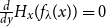 $\frac {d}{dy} H_x(f_\lambda (x)) =0$
, and that
 $H_x$
is increasing on
 $(x,f_\lambda (x))$
and decreasing on
 $(f_\lambda (x),1)$
. Also observe that, for
 $x\lt y\lt 1$
,
 \begin{align*} \frac {d^2}{dy^2} H_x(y) & = \frac 1y - \frac 1{1-y} - \frac 1{y-x} + \frac 1{\lambda +1-y} = - \frac {x}{y(y-x)} - \frac {\lambda }{(1-y)(\lambda +1-y)}\\ & \leq - \frac {\lambda }{(1-y)(\lambda +1-y)} \leq \frac {-\lambda }{\lambda +1}. \end{align*}
For the rest of the proof, fix
 $\varepsilon \gt 0$
. Assume
 $x \in (0,1)$
is such that
 $f_\lambda (x)\leq 1-\varepsilon$
. Applying Taylor’s theorem (with the Lagrange form of the remainder) yields that there exists
 $\zeta \in (x,1)$
such that
 \begin{equation*} H_{x}\left (f_\lambda (x) +\varepsilon \right ) = H_{x}\left (f_\lambda (x)\right ) + \varepsilon \frac {d}{dy}H_{x}\left (f_\lambda (x)\right ) + \frac {\varepsilon ^2}2 \frac {d^2}{dy^2}H_{x}\left (\zeta \right )\!. \end{equation*}
The previous observations about
 $H_x$
therefore yield
 \begin{equation*} H_{x}\left (f_\lambda (x) +\varepsilon \right ) = \frac {\varepsilon ^2}2 \frac {d^2}{dy^2}H_{x}\left (\zeta \right ) \leq \frac {-\lambda \varepsilon ^2}{2(\lambda +1)}. \end{equation*}
Similarly, assuming that
 $x \in (0,1)$
satisfies
 $f_\lambda (x)\geq \varepsilon$
, we get
 \begin{equation*} H_{x}\left (f_\lambda (x) -\varepsilon \right ) \leq \frac {-\lambda \varepsilon ^2}{2(\lambda +1)}. \end{equation*}
Using that
 $H_x$
is increasing until
 $y=f_\lambda (x)$
and then decreasing, it follows that, for
 $x \in (0,1)$
such that
 $\varepsilon \leq f_\lambda (x)\leq 1-\varepsilon$
, for all
 $y \in (x,f_\lambda (x)-\varepsilon ] \cup [f_\lambda (x)+\varepsilon ,1)$
,
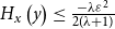 $H_{x}\left (y\right ) \leq \frac {-\lambda \varepsilon ^2}{2(\lambda +1)}$
, and thus
 \begin{equation} F(x,y) \leq \exp \left (\frac {-\lambda \varepsilon ^2}{2(\lambda +1)}\right )\!, \text{ a bound which does not depend on } x. \end{equation}
We can now conclude the proof of Proposition 26. We have that, for
 $n$
sufficiently large, for all
 $i \in \{1, \ldots , n\}$
such that
 $\varepsilon \lt f_\lambda (i/n) \lt 1-\varepsilon$
,
 \begin{align*} \mathbb{P}(|\textrm {lmax}(\sigma _n,i) & - nf_\lambda (i/n)|\gt \varepsilon \,n) \\ & = \sum _{j = 1}^{\lfloor nf_\lambda (i/n)-\varepsilon n\rfloor } \mathbb{P}(\textrm {lmax}(\sigma _n,i) = j) +\sum _{j = \lceil nf_\lambda (i/n)+\varepsilon n\rceil }^{n} \mathbb{P}(\textrm {lmax}(\sigma _n,i) = j) \\ & \leq n \cdot n^3 \cdot \exp \left (\frac {-\lambda \varepsilon ^2}{2(\lambda +1)}\right )^n, \end{align*}
where in the last line we used Lemma28 and Eq. (13). This proves the announced statement that, for
 $n$
sufficiently large,
 $\mathbb{P}\left (|\textrm {lmax}(\sigma _n,i) - nf_\lambda (i/n)|\gt \varepsilon \,n\right ) \leq c(\varepsilon )^n$
for all
 $i \in \{1, \ldots , n\}$
such that
 $\varepsilon \lt f_\lambda (i/n) \lt 1-\varepsilon$
, taking
 $c(\varepsilon )$
to be any value such that
 $ \exp \left ( \frac {-\lambda \varepsilon ^2}{2(\lambda +1)}\right )\lt c(\varepsilon )\lt 1$
.
Now that the concentration of
 $\textrm {lmax}(\sigma _n,i)$
has been established, we continue with our proof of Theorem25. We intend to use Lemma21 so that we will need to compare
 $\mu (R)$
and
 $\mu _n(R)$
for (grid-aligned) rectangles of the unit square having their bottom-left corner in
 $(0,0)$
. This set of rectangles is naturally divided into two subsets, as illustrated by Figure 15:
-
• the subset
$\mathcal{T}$
of tall rectangles consists of all rectangles
$R=[0,a]\times [0,b]$
such that
$b\geq f_\lambda (a)$
; -
• and the subset
$\mathcal{L}$
of long rectangles consists of all rectangles
$R=[0,a]\times [0,b]$
such that
$b\lt f_\lambda (a)$
.


A rectangle starting in the bottom-left corner is either tall or long.

Figure 15 Long description
A line graph compares tall and long rectangles. The graph features two rectangles, one tall and one long, with their dimensions labeled as 'a' and 'b'. The tall rectangle has a height greater than its width, while the long rectangle has a width greater than its height. A blue curve and a dashed black line represent different data trends. The x-axis and y-axis are not explicitly labeled, but the graph illustrates the relationship between the dimensions of the rectangles. All values are approximated.
With Proposition26, it is easy to compare
 $\mu _n(R)$
and
 $\mu (R)$
for tall rectangles.
Proposition 29. For every
 $\varepsilon \gt 0$
, there exists
 $c(\varepsilon ) \in (0,1)$
such that for
 $n$
sufficiently large we have, for any tall rectangle of the form
 $[0,i/n]\times [0,j/n]$
inside the unit square:
 \begin{equation*} \mathbb{P}\left (\left | \mu _n(R)-\mu (R)\right |\gt \varepsilon \right ) \leq c(\varepsilon )^n. \end{equation*}
Proof. Fix
 $\varepsilon \gt 0$
and some
 $n$
large enough. Consider a tall rectangle
 $R=[0,i/n]\times [0,j/n]$
inside the unit square. Assume first that
 $\varepsilon \lt f_\lambda (i/n) \lt 1-\varepsilon$
. From Proposition26, it is enough to show that
 \begin{equation*}\mathbb{P}\left (\left | \mu _n(R)-\mu (R)\right |\gt \varepsilon \right ) \leq \mathbb{P}\left (|\textrm {lmax}(\sigma _n,i) - nf_\lambda (i/n)|\gt \varepsilon \,n\right )\!.\end{equation*}
Because
 $R$
is a tall rectangle, by the uniform marginals property, we have
 $\mu (R) = i/n$
. And because
 $\mu _n$
is a permuton, it holds that
 $\mu _n(R) \leq i/n$
. Therefore,
 \begin{equation*}\mathbb{P}\left (\left | \mu _n(R)-\mu (R)\right |\gt \varepsilon \right ) = \mathbb{P}\left (\mu _n(R)\lt i/n - \varepsilon \right )\!.\end{equation*}
Recall that
 $\mu _n$
is the permuton associated to the permutation
 $\sigma _n$
(of size
 $n$
). Assuming
 $\mu _n(R)\lt i/n - \varepsilon$
means that
 $|\{k \leq i \,: \,\sigma _n(k) \leq j\}| \lt i - \varepsilon n$
, that is to say that
 $|\{k \leq i\, :\, \sigma _n(k) \gt j\}| \gt \varepsilon n$
. This last condition implies (by definition of
 $\textrm {lmax}$
) that
 $\textrm {lmax}(\sigma _n,i) \gt j + n\varepsilon$
. Since
 $R$
is a tall rectangle, we have
 $j/n \geq f_\lambda (i/n)$
so that
 $j + n\varepsilon \geq nf_\lambda (i/n) +\varepsilon n$
. Summing things up, assuming that
 $\mu _n(R)\lt i/n - \varepsilon$
implies that
 $\textrm {lmax}(\sigma _n,i) \gt nf_\lambda (i/n) +\varepsilon n$
. This shows that
 \begin{equation*} \mathbb{P}\left (\mu _n(R)\lt i/n - \varepsilon \right ) \leq \mathbb{P}\left (|\textrm {lmax}(\sigma _n,i) - nf_\lambda (i/n)|\gt \varepsilon \,n\right ) \end{equation*}
and therefore proves the proposition in the case where
 $\varepsilon \lt f_\lambda (i/n) \lt 1-\varepsilon$
.
If on the contrary
 $ f_\lambda (i/n) \leq \varepsilon$
or
 $f_\lambda (i/n) \geq 1-\varepsilon$
, let us show that
 $|\mu _n(R) - \mu (R)| \leq \varepsilon$
deterministically, which will conclude the proof. First, as we already observed,
 $\mu _n(R) \leq \mu (R) = i/n$
, so that we only need to show that
 $\mu (R) - \mu _n(R) \leq \varepsilon$
.
If
 $ f_\lambda (i/n) \leq \varepsilon$
, then by definition of
 $f_\lambda$
we have
 $i/n \leq f_\lambda (i/n) \leq \varepsilon$
so that
 $\mu (R) - \mu _n(R) \leq \mu (R) = i/n \leq \varepsilon$
.
The final case is when
 $f_\lambda (i/n) \geq 1-\varepsilon$
. Because
 $R$
is a tall rectangle, it holds that
 $j/n \geq f_\lambda (i/n)$
, so that
 $\varepsilon \geq 1 - j/n$
. Letting
 $S = [0,i/n]\times [0,1]$
, we observe that
 $\mu _n(S) = i/n$
because of the uniform marginals property of permutons. Since
 $S$
is the disjoint union of
 $R$
and
 $T=[0,i/n]\times [j/n,1]$
, it also holds that
 $\mu _n(R) = \mu _n(S) - \mu _n(T)$
. Lastly, we note that
 $\mu _n(T) \leq \mu _n([0,1]\times [j/n,1]) = 1-j/n$
again by the uniform marginals property. These observations allow us to write that
 $\mu (R) - \mu _n(R) = i/n - \mu _n(S) + \mu _n(T) = \mu _n(T) \leq 1-j/n \leq \varepsilon$
, concluding the proof.
We now turn to proving the analogue of Proposition29 for long rectangles (see Proposition33 below). The proof is more involved, and we present it using some intermediate statements.
Recall that, for integers
 $i,j \leq n$
, a rectangle
 $R = [0,i/n]\times [0,j/n]$
is long when
 $j/n \lt f_\lambda (i/n)$
. For such a rectangle, we introduce the following notation:
 $a=i/n$
,
 $b=j/n$
,
 $i'=\lfloor nf_\lambda ^{-1}(b)\rfloor$
, and
 $a'=i'/n$
. We also define the rectangles
 $R_1 = [0,a']\times [0,b]$
,
 $R_2 = [a'+1/n,a]\times [0,b]$
and
 $R_{\text{small}} = [a',a'+1/n]\times [0,b]$
(see Figure 16). Observe that
 $R_1$
is a tall rectangle, that
 $R_2$
entirely lies under the curve of
 $f_\lambda$
, and that
 $R$
is the disjoint union of
 $R_1$
,
 $R_2$
and
 $R_{\text{small}}$
. In addition, because of the uniform marginals property of permutons,
 $\nu (R_{\text{small}}) \leq 1/n$
for any permuton
 $\nu$
.
Partition of a long rectangle
 $R$
into
 $R_1 \uplus R_{\text{small}} \uplus R_2$
.

Figure 16 Long description
A line graph illustrates the partition of a long rectangle labeled R into three distinct regions. The regions are labeled R 1, R small, and R 2. The graph features a blue line representing a boundary that intersects the rectangle, dividing it into these regions. A red rectangle labeled R small is positioned at the top left corner, with a green dot marking an intersection point. The regions R 1 and R 2 are separated by a vertical red line, and a dashed black line extends diagonally across the graph. The x-axis is labeled with a and a prime, while the y-axis is labeled with b. The graph visually represents the division of the rectangle into the specified regions.
In addition, for any
 $\varepsilon \gt 0\in (0,1/2)$
, and any long rectangle as above, we define, for all integers
 $t$
such that
 $|t-nf_\lambda (a')|\leq \varepsilon ^2 n$
, the rectangle
 $R_t =[a'+1/n,a]\times [0,t/n]$
. Observe that, because
 $t/n$
is close to
 $f_\lambda (a')$
,
 $R_t$
does not differ much from
 $R_2$
.
Recall that
 $\sigma _n$
denotes a random record-biased permutation of size
 $n$
, for the parameter
 $\theta = \lambda n$
, and that
 $\mu _n$
denotes the permuton associated with
 $\sigma _n$
. Recall also that for
 $i\in [n]$
,
 $\textrm {lmax}(\sigma _n,i)=\max \{\sigma (j) \,:\,j\in [i]\}$
denotes the last (and largest) record occurring at or before position
 $i$
.
Our strategy to prove Proposition33 is the following. First, in Proposition30 we write
 $\mathbb{P}\left (|\mu _n(R)-\mu (R)|\gt 30\,\varepsilon \right )$
as a sum of two terms, according to whether
 $\textrm {lmax}(\sigma _n,i')$
is close or far from its typical value, and we establish an exponentially small bound for the latter case. Then, in Proposition31, we analyse the former case to also prove that it is exponentially small, relying on a technical statement given in Lemma32.
Proposition 30. For any
 $\varepsilon \in (0,1/2)$
, there exists
 $c(\varepsilon ) \in (0,1)$
such that, for
 $n$
sufficiently large and for any long rectangle
 $R=[0,i/n]\times [0,j/n]$
inside the unit square, using the notation
 $i'=\lfloor nf_\lambda ^{-1}(j/n)\rfloor$
, and
 $a'=i'/n$
introduced above, we have:
 \begin{align*} & \mathbb{P}\left (|\mu _n(R)-\mu (R)|\gt 30\,\varepsilon \right ) \\ & \qquad \leq \sum _{t \text{ s.t. } \atop {|t-nf_\lambda (a')|\leq \varepsilon ^2 n}} \hspace {-0.6cm}\mathbb{P}\left (|\mu _n(R_t)-\mu (R_t)|\gt 8 \,\varepsilon \mid {\operatorname{lmax}}(\sigma _n,i')=t\right ) \cdot \mathbb{P}({\operatorname{lmax}}(\sigma _n,i')=t) + c(\varepsilon )^n. \end{align*}
Proof. Let us first prove the statement when
 $f_\lambda (i'/n) \lt \varepsilon ^2$
. Recalling that
 $i'=\lfloor nf_\lambda ^{-1}(j/n)\rfloor$
and that
 $f_\lambda$
is increasing, we write that
 \begin{equation*} \frac {i'}{n} = \frac {1}{n} \lfloor nf_\lambda ^{-1}(j/n)\rfloor \geq \frac {1}{n} \left ( nf_\lambda ^{-1}(j/n) -1 \right ) = f_\lambda ^{-1}(j/n) -1/n, \end{equation*}
so that
 $j/n \leq f_\lambda (\tfrac {i'+1}{n})$
. By the mean value theorem, and since
 $\max _{x\in [0,1]} |f_\lambda '(x)| = f_\lambda '(0) = \tfrac {\lambda +1}\lambda$
, under the assumption that
 $f_\lambda (i'/n) \lt \varepsilon ^2$
, we have, for
 $n$
large enough,
 \begin{equation*} f_\lambda \bigg(\frac {i'+1}{n}\bigg) \leq f_\lambda (i'/n) + \frac {1}{n} \frac {\lambda +1}\lambda \leq 2 \varepsilon ^2 \leq \varepsilon \end{equation*}
(where we used the assumption that
 $\varepsilon \in (0,1/2)$
for the last inequality). It follows that for any permuton
 $\nu$
,
 $\nu (R) \leq j/n \leq \varepsilon$
. Therefore,
 $|\mu _n(R)-\mu (R)| \leq 2 \varepsilon$
, so that
 $\mathbb{P}\left (|\mu _n(R)-\mu (R)|\gt 30\,\varepsilon \right ) =0$
, which obviously implies our proposition in this particular case.
For the rest of the proof, let us then assume that
 $f_\lambda (i'/n) \geq \varepsilon ^2$
. Writing
 $R$
as
 $R_1 \uplus R_{\text{small}} \uplus R_2$
, we first derive that
 \begin{align*} \mathbb{P}\left (|\mu _n(R)-\mu (R)|\gt 30\,\varepsilon \right ) & \leq \mathbb{P}\left (|\mu _n(R_1)-\mu (R_1)|\gt 10\,\varepsilon \right )\\ & + \mathbb{P}\left (|\mu _n(R_{\text{small}})-\mu (R_{\text{small}})|\gt 10\,\varepsilon \right )\\ & + \mathbb{P}\left (|\mu _n(R_2)-\mu (R_2)|\gt 10\,\varepsilon \right ). \end{align*}
Because
 $R_1$
is a tall rectangle, we know from Proposition29 that there exists
 $c_{\text{tall}}(\varepsilon ) \in (0,1)$
independent of
 $R$
such that, for
 $n$
sufficiently large
 $\mathbb{P}\left (|\mu _n(R_1)-\mu (R_1)|\gt 10\,\varepsilon \right ) \leq c_{\text{tall}}(\varepsilon )^n$
. In addition,
 $|\mu _n(R_{\text{small}})-\mu (R_{\text{small}})| \leq 2/n$
; as a consequence, it holds that for
 $n$
sufficiently large,
 $\mathbb{P}\left (|\mu _n(R_{\text{small}})-\mu (R_{\text{small}})|\gt 10\,\varepsilon \right ) =0$
. We therefore focus on
 $\mathbb{P}\left (|\mu _n(R_2)-\mu (R_2)|\gt 10\,\varepsilon \right )$
.
Again, we distinguish a special case, this time when
 $f_\lambda (i'/n) \gt 1 - \varepsilon ^2$
. From
 $i'=\lfloor nf_\lambda ^{-1}(j/n)\rfloor$
and the increasing property of
 $f_\lambda$
, we first derive that
 $f_\lambda (i'/n) \leq j/n$
, so that
 $1-j/n \leq \varepsilon ^2$
. We now define the rectangles
 $S=[\tfrac {i'+1}{n},\tfrac {i}{n}]\times [0,1]$
and
 $T=[\tfrac {i'+1}{n},\tfrac {i}{n}]\times [j/n,1]$
, which satisfy that
 $S = R_2 \uplus T$
. Note that, for any permuton
 $\nu$
, by the uniform marginals property, we have
 $\nu (S) = \tfrac {i-i'-1}{n}$
and
 $\nu (T) \leq 1-j/n$
. Therefore,
 \begin{equation*} |\mu _n(R_2)-\mu (R_2)| = |\mu _n(S)-\mu _n(T) - \mu (S)+\mu (T)| = |\mu (T) - \mu _n(T)| \leq 2 \cdot (1-j/n) \leq 2\varepsilon ^2\leq \varepsilon . \end{equation*}
Consequently,
 $\mathbb{P}\left (|\mu _n(R_2)-\mu (R_2)|\gt 10\,\varepsilon \right ) = 0$
in this case.
We are now left with providing an upper bound on
 $\mathbb{P}\left (|\mu _n(R_2)-\mu (R_2)|\gt 10\,\varepsilon \right )$
, when the inequalities
 $\varepsilon ^2 \leq f_\lambda (i'/n) \leq 1 - \varepsilon ^2$
are satisfied. We use the law of total probability to write that
 \begin{align*} \mathbb{P}\left (|\mu _n(R_2){-}\mu (R_2)|\gt 10\,\varepsilon \right ) & \! = \sum _{t = 1}^n \mathbb{P}\left (|\mu _n(R_2){-}\mu (R_2)|\gt\! 10 \,\varepsilon \!\mid\! \textrm {lmax}(\sigma _n,i') = t\right ) \cdot \mathbb{P}(\textrm {lmax}(\sigma _n,i') = t{}) \\ & \leq \hspace {-0.6cm} \sum _{t \text{ s.t. } \atop {|t{-}nf_\lambda (a')|\leq \varepsilon ^2 n}} \hspace {-0.6cm}\mathbb{P}\left (|\mu _n(R_2){-}\mu (R_2)|\gt\! 10 \,\varepsilon \!\mid\! \textrm {lmax}(\sigma _n,i')=t\right ) \cdot \mathbb{P}(\textrm {lmax}(\sigma _n,i')=t) \\ & + \hspace {-0.6cm} \sum _{t \text{ s.t. } \atop {|t{-}nf_\lambda (a')| \gt \varepsilon ^2 n}} \hspace {-0.6cm} \mathbb{P}(\textrm {lmax}(\sigma _n,i') = t). \end{align*}
For the term
 $\sum _{t}\mathbb{P}(\textrm {lmax}(\sigma _n,i')=t)$
with the index
 $t$
ranging on values such that
 $|t-nf_\lambda (a')| \gt \varepsilon ^2 n$
, we shall use Proposition26. Indeed, since it holds that
 $\varepsilon ^2 \leq \, f_\lambda (i'/n) \leq 1 - \varepsilon ^2$
, we can write that, for
 $n$
sufficiently large,
 \begin{equation*} \hspace {-0.6cm} \sum _{t \text{ s.t. } \atop {|t-nf_\lambda (a')| \gt \varepsilon ^2 n}} \hspace {-0.6cm} \mathbb{P}(\textrm {lmax}(\sigma _n,i')=t) = \mathbb{P}(|\textrm {lmax}(\sigma _n,i')-nf_\lambda (i'/n)| \gt \varepsilon ^2 n) \leq c(\varepsilon ^2)^n \end{equation*}
for the constant
 $c(\varepsilon ^2)$
given by Proposition26. As a consequence, there exists
 $c_{2}(\varepsilon )$
such that, for
 $n$
large enough,
 \begin{equation*} \hspace {-0.6cm} \sum _{t \text{ s.t. } \atop {|t-nf_\lambda (a')| \gt \varepsilon ^2 n}} \hspace {-0.6cm} \mathbb{P}(\textrm {lmax}(\sigma _n,i')=t) \leq c_2(\varepsilon )^n. \end{equation*}
Putting things together, to conclude the proof, it is enough to show that, for any integer
 $t$
such that
 $|t-nf_\lambda (a')| \leq \varepsilon ^2 n$
,
 \begin{equation*} \mathbb{P}\left (|\mu _n(R_2)-\mu (R_2)|\gt 10 \,\varepsilon \mid \textrm {lmax}(\sigma _n,i')=t\right ) \leq \mathbb{P}\left (|\mu _n(R_t)-\mu (R_t)|\gt 8 \,\varepsilon \mid \textrm {lmax}(\sigma _n,i')=t\right ). \end{equation*}
Let us fix some integer
 $t$
such that
 $|t-nf_\lambda (a')|\leq \varepsilon ^2 n$
. Recall that
 $R_t = [a'+1/n,a]\times [0,t/n]$
and
 $R_2 = [a'+1/n,a]\times [0,b]$
. Consequently, if
 $t/n \leq b$
then
 $R_2 = R_t \uplus [a'+1/n,a]\times [t/n,b]$
and otherwise
 $R_t = R_2 \uplus [a'+1/n,a]\times [b,t/n]$
. Therefore, for any permuton
 $\nu$
, we have
 \begin{equation*} |\nu (R_2)-\nu (R_t)| \leq |b-t/n|. \end{equation*}
Next, using the assumption that
 $|t-nf_\lambda (a')|\leq \varepsilon ^2 n$
and the fact that
 $f_\lambda (a')\leq b \leq f_\lambda (a'+1/n)$
, we have
 \begin{equation*} |b-t/n| \leq |b-f_\lambda (a')| + \varepsilon ^2 \leq |f_\lambda (a'+1/n)-f_\lambda (a')| + \varepsilon ^2. \end{equation*}
Using again the mean value theorem, and recalling that
 $\max _{x\in [0,1]} |f_\lambda '(x)| = \frac {\lambda +1}\lambda$
, we obtain that
 $|f_\lambda (a'+1/n)-f_\lambda (a')|\leq \frac {\lambda +1}{\lambda n}$
. Hence, recalling our assumption that
 $\varepsilon \in (0,\frac 12)$
, for
 $n$
sufficiently large, and for any permuton
 $\nu$
,
 \begin{equation} |\nu (R_2)-\nu (R_t)| \leq |b-t/n| \leq \frac {\lambda +1}{\lambda n} + \varepsilon ^2 \leq 2\,\varepsilon ^2 \leq \varepsilon . \end{equation}
Using the above for
 $\nu =\mu$
and
 $\nu = \mu _n$
, it follows that
 \begin{equation*} \left |\mu _n(R_2) - \mu (R_2)\right |\gt 10\,\varepsilon \Rightarrow \left |\mu _n(R_t) - \mu (R_t)\right |\gt 8\,\varepsilon , \end{equation*}
and the above holds deterministically. This proves that
 \begin{equation*} \mathbb{P}\left (|\mu _n(R_2)-\mu (R_2)|\gt 10 \,\varepsilon \mid \textrm {lmax}(\sigma _n,i')=t\right ) \leq \mathbb{P}\left (|\mu _n(R_t)-\mu (R_t)|\gt 8 \,\varepsilon \mid \textrm {lmax}(\sigma _n,i')=t\right )\!, \end{equation*}
hence concluding the proof.
Proposition 31. For any
 $\varepsilon \in (0,1/2)$
, there exists
 $c(\varepsilon ) \in (0,1)$
such that, for
 $n$
sufficiently large and for any long rectangle
 $R=[0,i/n]\times [0,j/n]$
inside the unit square, using the notation
 $i'=\lfloor nf_\lambda ^{-1}(j/n)\rfloor$
, and
 $a'=i'/n$
introduced above, for any integer
 $t$
such that
 $|t-nf_\lambda (a')|\leq \varepsilon ^2 n$
, the rectangle
 $R_t = [a'+1/n,a]\times [0,t/n]$
satisfies:
 \begin{equation*} \mathbb{P}\left (|\mu _n(R_t)-\mu (R_t)|\gt 8 \,\varepsilon \mid {\operatorname{lmax}}(\sigma _n,i')=t\right ) \leq c(\varepsilon )^n. \end{equation*}
To prove the above, we use a large deviation result, stated in the following lemma. Its proof follows the same structure as that of Proposition26 and is differed to the end of this section.
Lemma 32.
For any positive integers
 $k$
,
 $\ell$
and
 $n$
, such that
 $\ell \leq n$
and
 $k\leq n$
, let us denote by
 $X_{\ell ,n,k}$
the random variable that counts the number of integers smaller than or equal to
 $\ell$
in a uniform random size-
 $k$
subset of
 $[n]$
.
For any
 $\varepsilon \gt 0$
, there exists
 $c(\varepsilon ) \in (0,1)$
such that, for
 $n$
sufficiently large, for all
 $1\leq \ell , k \leq n$
,
 \begin{equation*} \mathbb{P}\left (\left |X_{\ell ,n,k}-\frac {\ell k}{n} \right |\gt \varepsilon n\right ) \leq c(\varepsilon )^n. \end{equation*}
Proof of Proposition 31. We start by computing
 $\mu (R_t)$
, or rather finding a good estimate for it. Recall from Eq. (14) that, under the assumptions that
 $\varepsilon \in (0,1/2)$
and
 $|t-nf_\lambda (a')|\leq \varepsilon ^2 n$
, it holds that
 $|b-t/n| \leq \varepsilon$
. By definition, we also have that
 $f_\lambda (a'+1/n) \geq b$
.
In the case that
 $f_\lambda (a'+1/n) \gt t/n$
,
 $\mu (R_t)$
is easily computed. Indeed, then
 $R_t$
lies entirely under the curve of
 $f_\lambda$
, so that
 $\mu (R_t)$
is proportional to its area; namely,
 $\mu (R_t) = \tfrac {(a-(a'+1/n))t}{(\lambda +1)n}$
. If on the contrary
 $f_\lambda (a'+1/n) \leq t/n$
, then
 $R_t$
is not entirely under the curve of
 $f_\lambda$
, but almost. More precisely, in this case we have
 $0\leq t/n - f_\lambda (a'+1/n) \leq t/n -b \leq \varepsilon$
, from which we derive (using again the uniform marginal property of permutons) that
 $\mu (R_t) \leq \tfrac {(a-(a'+1/n))t}{(\lambda +1)n} + \varepsilon$
. Therefore, in both cases, it holds that
 \begin{equation*} \left |\mu (R_t) - \tfrac {(a-(a'+1/n))t}{(\lambda +1)n} \right | \leq \varepsilon . \end{equation*}
As a consequence, Proposition31 will follow if we show that there exists
 $c(\varepsilon )\in (0,1)$
that only depends on
 $\varepsilon$
such that for
 $n$
sufficiently large, it holds that
 \begin{equation} \mathbb{P}\left (\left |\mu _n(R_t) - \frac {(i-i'-1)t}{(\lambda +1)n^2} \right | \gt 7\,\varepsilon \mid \textrm {lmax}(\sigma _n,i')=t\right ) \leq c(\varepsilon )^n. \end{equation}
To prove Eq. (15), we express
 $\mu _n(R_t)$
by a quantity defined from the permutation
 $\sigma _n$
directly. Indeed,
 $R_t$
has its sides supported by the
 $n \times n$
grid inside the unit square. This implies that
 $\mu _n(R_t) = \tfrac {1}{n} \cdot \rho _{i',i}^t(\sigma _n)$
where, for any permutation
 $\sigma$
of size
 $n$
, we define
 $\rho _{i',i}^t(\sigma )$
as the number of elements
 $x$
of
 $\{i'+1, i'+2,\ldots , i-1\}$
such that
 $\sigma (x) \leq t$
. Eq. (15) can therefore be rewritten as
 \begin{equation} \mathbb{P}\left (\left |\rho _{i',i}^t(\sigma _n)-\frac {t(i-i'-1)}{(\lambda +1)n}\right |\gt 7\,\varepsilon \,n\mid \textrm {lmax}(\sigma _n,i')=t\right ) \leq c(\varepsilon )^n. \end{equation}
We now describe the structure of permutations of size
 $n$
satisfying the condition
 $\textrm {lmax}(\sigma ,i')=t$
, which is equivalently written as
 $\max _{x\in [i']}\sigma (x) = t$
. Such a permutation is entirely characterised by the data of
-
• a subset
$T \in [t]$
of size
$i'$
containing
$t$
, together with a bijective mapping
$\phi _{\text{left}}$
from
$[i']$
to
$T$
(this describes
$\sigma ([i']) =T$
and the permutation of these values occurring in the prefix of length
$i'$
of
$\sigma$
); -
• a subset
$A$
of size
$t-i'$
of
$\{i'+1, \ldots , n\}$
, together with a bijective mapping
$\phi _{\text{right,small}}$
from
$A$
to
$S = [t] \setminus T$
(this describes the points of
$\sigma$
occurring after position
$i'$
that have a value less than
$t$
, as well as their images by
$\sigma$
); -
• a bijective mapping
$\phi _{\text{right,large}}$
from
$B = \{i'+1, \ldots , n\} \setminus A$
to
$\{t+1, \ldots , n\}$
(this describes
$\sigma$
restricted to positions larger than
$i'$
and values larger than
$t$
).


Observe that, for a permutation
 $\sigma$
as above,
 $\rho _{i',i}^t(\sigma ) = |A \cap [i'+1, i-1]|$
. In addition, the number of records of a permutation
 $\sigma$
as above depends only on
 $\phi _{\text{left}}$
and
 $\phi _{\text{right,large}}$
. In particular, for
 $\sigma _n$
a record-biased permutation of size
 $n$
, and under the condition that
 $\textrm {lmax}(\sigma _n,i')=t$
, the set
 $A$
defined above is a uniform random subset of size
 $t-i'$
of
 $\{i'+1, \ldots , n\}$
. As a consequence, using the notation of Lemma32,
 $\rho _{i',i}^t(\sigma _n)$
is equal in distribution to
 $X_{i-1-i', n-i', t-i'}$
under the conditioning
 $\textrm {lmax}(\sigma _n,i')=t$
. The strategy to prove Eq. (16) is then to use Lemma32, but it only applies when
 $n-i'$
tends to infinity. We therefore start by discarding the cases where
 $i'$
is too large.
First observe that, for
 $\sigma$
a permutation of size
 $n$
such that
 $\textrm {lmax}(\sigma ,i')=t$
, by definition we have
 $\rho _{i',i}^t(\sigma ) \leq n-i'$
, from which we deduce
 \begin{equation*} \left |\rho _{i',i}^t(\sigma ) - \frac {t(i-i'-1)}{(\lambda +1)n}\right | \leq \rho _{i',i}^t(\sigma ) + \frac {n(n-i')}{(\lambda +1)n} \leq \frac {\lambda +2}{\lambda +1}(n-i') \leq 2(n-i'). \end{equation*}
Therefore, if
 $i'\geq n-3\varepsilon n$
, then
 $\mathbb{P}\left (\left |\rho _{i',i}^t(\sigma _n)-\frac {t(i-i'-1)}{(\lambda +1)n}\right |\gt 7\,\varepsilon \,n\mid \textrm {lmax}(\sigma _n,i')=t\right ) = 0$
, proving our claim in this case. For the rest of the proof, let us then assume that
 $i'\lt n-3\varepsilon n$
, that is to say
 $n-i' \gt 3\varepsilon n$
. In particular, for any fixed
 $\varepsilon \in (0,1/2)$
,
 $n-i'$
tends to infinity when
 $n$
does. Applying Lemma32 (with
 $4\varepsilon$
instead of
 $\varepsilon$
), we have that there exists
 $c_X(\varepsilon ) \in (0,1)$
depending only on
 $\varepsilon$
such that, for
 $n$
sufficiently large,
 \begin{equation*} \mathbb{P}\left (\left |\rho _{i',i}^t(\sigma _n)-\frac {(t-i')(i-i'-1)}{n-i'}\right |\gt 4\,\varepsilon \,(n-i')\mid \textrm {lmax}(\sigma _n,i')=t\right ) \leq c_X(\varepsilon )^{n-i'}\leq c_X(\varepsilon )^{3\varepsilon n}, \end{equation*}
which implies
 \begin{equation} \mathbb{P}\left (\left |\rho _{i',i}^t(\sigma _n)-\frac {(t-i')(i-i'-1)}{n-i'}\right |\gt 4\,\varepsilon \,n\mid \textrm {lmax}(\sigma _n,i')=t\right )\leq c_X(\varepsilon )^{3\varepsilon n}. \end{equation}
This resembles Eq. (16) which we want to prove: the differences are that the fraction
 $\frac {(t-i')(i-i'-1)}{n-i'}$
in Eq. (17) is replaced by
 $\frac {t(i-i'-1)}{(\lambda +1)n}$
in Eq. (16), and that we allow ourselves
 $7 \, \varepsilon \, n$
in Eq. (16) instead of
 $4 \, \varepsilon \, n$
in Eq. (17).
To prove Eq. (16) from Eq. (17), we shall use small upper bounds of several differences, which we now give. Recall from Eq. (14) that
 $|t/n - b| \leq 2 \varepsilon ^2$
for
 $n$
large enough. Therefore (recalling also that
 $\varepsilon \in (0,1/2$
)), for
 $n$
sufficiently large, it holds that
 \begin{equation} \left |\frac {t(i-i'-1)}{(\lambda +1)n}-\frac {b(i-i'-1)}{(\lambda +1)}\right | = \left |\frac {t}n - b\right |\cdot \frac {i-i'-1}{\lambda +1} \leq 2\,\varepsilon ^2 n \leq \varepsilon n. \end{equation}
In addition, using that
 $n-i'\geq 3\,\varepsilon n$
, we also have, for
 $n$
sufficiently large
 \begin{equation} \left |\frac {(t-i')(i-i'-1)}{n-i'}-\frac {(bn-i')(i-i'-1)}{n-i'}\right | =n\cdot \left |\frac {t}n-b\right |\cdot \frac {i-i'-1}{n-i'}\leq n\cdot 2\,\varepsilon ^2\frac {n}{3\,\varepsilon \,n}\leq \varepsilon n. \end{equation}
For the other two estimates that we need, it is convenient to introduce the notation
 $\beta = f_{\lambda }^{-1}(b)$
. Because
 $i'$
is defined as
 $i'=\lfloor nf_\lambda ^{-1}(b)\rfloor$
, we have
 $i'/n \leq \beta \leq (i'+1)/n$
. In addition, since
 $i'\lt n-3\varepsilon n$
, it holds that
 $\beta \leq 1- 3 \varepsilon + 1/n \leq 1- 2 \varepsilon$
for
 $n$
large enough. Consequently, for
 $n$
sufficiently large, we have
 \begin{equation*} \frac {bn-i'}{n-i'} = \frac {b-i'/n}{1-i'/n} \leq \frac {b-\beta +1/n}{1-\beta } = \frac {b-\beta }{1-\beta } +\frac {1}{1-\beta } \frac {1}{n} \leq \frac {b-\beta }{1-\beta } +\frac {1}{2 \varepsilon } \frac {1}{n}\leq \frac {b-\beta }{1-\beta } +\varepsilon . \end{equation*}
Therefore, for
 $n$
sufficiently large,
 \begin{equation} \left |\frac {(bn-i')(i-i'-1)}{n-i'} - \frac {(b-\beta )(i-i'-1)}{1-\beta } \right | \leq \varepsilon \, n. \end{equation}
Finally, since
 $b = f_\lambda (\beta ) = \frac {\beta (\lambda +1)}{\lambda +\beta }$
, we have
 \begin{equation} \frac {b}{\lambda +1} = \frac {b- \beta }{1-\beta }. \end{equation}
Indeed, this can for example be derived from
 \begin{align*} b = \frac {\beta (\lambda +1)}{\lambda +\beta }& \Leftrightarrow \frac {b}{\lambda +1}=\frac {\beta }{\lambda +\beta } \ \Leftrightarrow \ b(\lambda +\beta ) = \beta (\lambda +1)\ \Leftrightarrow \ (b-\beta )\lambda = \beta -b\beta \\ & \Leftrightarrow (b-\beta )(\lambda +1)= \beta -b\beta + (b-\beta ) = (1-\beta )b \ \Leftrightarrow \ \frac {b}{\lambda +1} = \frac {b-\beta }{1-\beta }. \end{align*}
Combining Eq. (18) to Eq. (21), we derive that, for
 $n$
sufficiently large,
 \begin{align*} \left |\rho _{i',i}^t(\sigma _n)-\frac {t(i-i'-1)}{(\lambda +1)n}\right |\gt 7\,\varepsilon \,n & \Rightarrow \left |\rho _{i',i}^t(\sigma _n)-\frac {b(i-i'-1)}{\lambda +1}\right |\gt 6\,\varepsilon \,n \qquad \text{from (18)} \\ & \Rightarrow \left |\rho _{i',i}^t(\sigma _n)-\frac {(b-\beta )(i-i'-1)}{1-\beta }\right |\gt 6\,\varepsilon \,n \qquad \text{from (20)}\\ & \Rightarrow \left |\rho _{i',i}^t(\sigma _n)-\frac {(bn-i')(i-i'-1)}{n-i'}\right |\gt 5\,\varepsilon \,n \qquad \text{from (21)}\\ & \Rightarrow \left |\rho _{i',i}^t(\sigma _n)-\frac {(t-i')(i-i'-1)}{n-i'}\right |\gt 4\,\varepsilon \,n \qquad \text{from (19)}. \end{align*}
As a consequence, for
 $n$
sufficiently large, it holds that
 \begin{align*} & \mathbb{P}\left (\left |\rho _{i',i}^t(\sigma _n)-\frac {t(i-i'-1)}{(\lambda +1)n}\right |\gt 7\,\varepsilon \,n\mid \textrm {lmax}(\sigma _n,i')=t\right ) \\ & \qquad \leq \mathbb{P}\left (\left |\rho _{i',i}^t(\sigma _n)-\frac {(t-i')(i-i'-1)}{n-i'}\right |\gt 4\,\varepsilon \,n\mid \textrm {lmax}(\sigma _n,i')=t\right ), \end{align*}
and our proposition follows from the above and Eq. (17).
With Propositions30 and 31 in our hands, the desired large deviation result for long rectangles is easily derived.
Proposition 33. For every
 $\varepsilon \in (0,1/2)$
, there exists
 $c(\varepsilon ) \in (0,1)$
such that for
 $n$
sufficiently large we have, for any long rectangle
 $R=[0,i/n]\times [0,j/n]$
inside the unit square:
 \begin{equation*} \mathbb{P}\left (\left | \mu _n(R)-\mu (R)\right |\gt 30\varepsilon \right ) \leq c(\varepsilon )^n. \end{equation*}
Proof. From Proposition30, we know that there exists
 $c_{30}(\varepsilon )$
such that for any long rectangle
 $R=[0,i/n]\times [0,j/n]$
inside the unit square, for
 $n$
large enough,
 \begin{align*} & \mathbb{P}\left (|\mu _n(R)-\mu (R)|\gt 30\,\varepsilon \right ) \\ & \qquad \leq \sum _{t \text{ s.t. } \atop {|t-nf_\lambda (a')|\leq \varepsilon ^2 n}} \hspace {-0.6cm}\mathbb{P}\left (|\mu _n(R_t)-\mu (R_t)|\gt 8 \,\varepsilon \mid \textrm {lmax}(\sigma _n,i')=t\right ) \cdot \mathbb{P}(\textrm {lmax}(\sigma _n,i')=t) + c_{30}(\varepsilon )^n. \end{align*}
Then, Proposition31 gives us a constant
 $c_{31}(\varepsilon )$
such that, for any long rectangle
 $R=[0,i/n]\times [0,j/n]$
inside the unit square, and for any
 $t$
such that
 $|t-nf_\lambda (a')|\leq \varepsilon ^2 n$
, the rectangle
 $R_t$
satisfies that, for
 $n$
large enough,
 \begin{equation*} \mathbb{P}\left (|\mu _n(R_t)-\mu (R_t)|\gt 8 \,\varepsilon \mid \textrm {lmax}(\sigma _n,i')=t\right ) \leq c_{31}(\varepsilon )^n. \end{equation*}
It follows that there exists
 $c(\varepsilon )$
such that for
 $n$
large enough,
 \begin{equation*} \mathbb{P}\left (|\mu _n(R)-\mu (R)|\gt 30\,\varepsilon \right ) \leq n c_{31}(\varepsilon )^n + c_{30}(\varepsilon )^n \leq c(\varepsilon )^n. \end{equation*}
Combining Propositions29 and 33 (large deviation results for tall and long rectangles), we can conclude the proof of the convergence of
 $\mu _n$
to
 $\mu$
, as stated in Theorem25.
Proof of Theorem 25. From Lemma21, it is enough to show that, for every
 $\varepsilon \in (0,1/2)$
, we have
 ${\mathbb{P}}(d_{\cdot /n} (\mu _n, \mu )\gt \varepsilon ) \to 0$
as
 $n \to \infty$
. Let us recall that the distance
 $d_{\cdot /n}$
is defined by
 $d_{\cdot /n}(\mu , \nu ) = \sup (|\mu (R)-\nu (R)|)$
where
 $R$
ranges over the family
 $\mathcal{R}_n$
of rectangles of the form
 $[0,i/n]\times [0,j/n]$
, for
 $0\leq i,j \leq n$
. Using the union bound, we obtain
 \begin{equation*} {\mathbb{P}}(d_{\cdot /n}(\mu _n , \mu ) \gt \varepsilon ) \leq \sum _{R \in \mathcal{R}_n} {\mathbb{P}}(|\mu _n(R)-\mu (R)| \gt \varepsilon ). \end{equation*}
Since there are only
 $\mathcal{O}(n^2)$
rectangles in
 $\mathcal{R}_n$
, all of which are either long or tall, Propositions29 and 33 ensure that
 ${\mathbb{P}}(d_{\cdot /n}(\mu _n , \mu ) \gt \varepsilon )$
indeed tends to
 $0$
as
 $n$
tends to infinity (and even at exponential speed).
We finish by giving the proof of Lemma 32, as announced above.
Proof of Lemma 32. We first shrink the range of useful values for our parameters, as we are only interested in bounding from above
 $\mathbb{P}(|X_{\ell ,n,k}-\frac {\ell k}n|\gt \varepsilon n)$
. Since
 $X_{\ell ,n,k}\leq \ell \leq n$
and
 $X_{\ell ,n,k}\leq k\leq n$
, if either
 $k$
or
 $\ell$
is smaller than
 $\varepsilon n$
, then
 $X_{\ell ,n,k}-\frac {\ell k}n \leq X_{\ell ,n,k}\leq \varepsilon n$
and
 $\frac {\ell k}n - X_{\ell ,n,k} \leq \frac {\ell k}n \leq \varepsilon n$
. Hence, in these cases,
 $\mathbb{P}(|X_{\ell ,n,k}-\frac {\ell k}n|\gt \varepsilon n) = 0$
.
Assume now that
 $\ell \geq n-\varepsilon n$
. Then, out of
 $k$
random elements, at most
 $\varepsilon n$
are not in
 $[\ell ]$
. Therefore
 $X_{\ell ,n,k}\geq k-\varepsilon n$
, yielding
 $\frac {k\ell }n-X_{\ell ,n,k}\leq k -k +\varepsilon n\leq \varepsilon n$
. Also, as
 $X_{\ell ,n,k}\leq k$
we have
 $X_{\ell ,n,k}-\frac {k\ell }n\leq k - \frac {k\ell }n \leq k - \frac {k(n-\varepsilon n)}n \leq \varepsilon k\leq \varepsilon n$
. So in this case also,
 $\mathbb{P}(|X_{\ell ,n,k}-\frac {\ell k}n|\gt \varepsilon n) = 0$
. We can similarly prove that
 $k \geq n-\varepsilon n$
implies
 $\mathbb{P}(|X_{\ell ,n,k}-\frac {\ell k}n|\gt \varepsilon n) = 0$
. Thus, we only consider the cases where
 $\varepsilon n \leq k\leq n-\varepsilon n$
, and
 $\varepsilon n \leq \ell \leq n-\varepsilon n$
in the sequel.
Clearly,
 $\mathbb{P}(X_{\ell ,n,k} = r) = \frac {\binom {\ell }{r}\binom {n-\ell }{k-r}}{\binom {n}{k}}$
. This probability is
 $0$
if
 $r \gt \ell$
or
 $ r\gt k$
or
 $k-r\gt n-\ell$
, so we can assume that
 $\ell \geq r$
,
 $k \geq r$
and
 $r \geq k+\ell -n$
from now on. Using the (crude) Stirling bounds of Eq. (12) we have for any positive integers
 $a\gt b$
:
 \begin{equation*} \frac {a^a}{9a^2\cdot b^b(a-b)^{a-b}} \leq \binom {a}{b} \leq \frac {3a\cdot a^a}{b^b(a-b)^{a-b}}, \end{equation*}
so that
 \begin{equation*} \frac {\binom {\ell }{r}\binom {n-\ell }{k-r}}{\binom {n}{k}} \leq 81n^4 \frac {\ell ^\ell (n-\ell )^{n-\ell }k^k(n-k)^{n-k}}{r^r(\ell -r)^{\ell -r}(k-r)^{k-r}(n-\ell -k+r)^{n-\ell -k+r}n^n}. \end{equation*}
We define the function
 $\kappa$
on triples
 $(x,y,z) \in [0,1]^3$
such that
 $x-z\geq 0$
,
 $y-z\geq 0$
and
 $1-x-y+z \geq 0$
by
 \begin{equation*} \kappa (x,y,z) = \frac {x^x(1-x)^{1-x}y^y(1-y)^{1-y}}{z^z(x-z)^{x-z}(y-z)^{y-z}(1-x-y+z)^{1-x-y+z}}, \end{equation*}
with the convention that
 $0^0 =1$
. Setting
 $x=\ell /n$
,
 $y=k/n$
and
 $z=r/n$
, the previous inequality can be rewritten as
 \begin{equation*} \frac {\binom {\ell }{r}\binom {n-\ell }{k-r}}{\binom {n}{k}} \leq 81\cdot n^4 \cdot \kappa \left (\frac {\ell }n,\frac {k}n,\frac {r}n\right )^n. \end{equation*}
A lower bound can be derived similarly. Putting things together yields that, for
 $n$
sufficiently large,
 \begin{equation} \frac 1{n^6}\cdot \kappa \left (\frac {\ell }n,\frac {k}n,\frac {r}n\right )^n \leq \mathbb{P}(X_{\ell ,n,k} = r) \leq n^5\cdot \kappa \left (\frac {\ell }n,\frac {k}n,\frac {r}n\right )^n. \end{equation}
Using the assumptions
 $\varepsilon n \leq k, \ell \leq n - \varepsilon n$
described earlier in the proof, we are only interested in
 $\kappa (x,y,z)$
for
 $x,y\in [\varepsilon ,1-\varepsilon ]$
.
For given
 $x,y\in [\varepsilon , 1-\varepsilon ]$
we consider the real-valued map
 $\kappa _{x,y}: z\mapsto \kappa (x,y,z)$
defined on the (nonempty) interval
 $ I=[\max \{0,x+y-1\},\min \{x,y\}]$
. This map is continuous, and infinitely differentiable on
 $\mathring {I}=(\max \{0,x+y-1\},\min \{x,y\})$
. Simple computations yield:
 \begin{equation*} \frac {d}{dz}\log \kappa _{x,y}(z) = \log \frac {(x-z)(y-z)}{z(1-x-y+z)}.\end{equation*}
Observe that
 \begin{equation*} \frac {d}{dz}\log \kappa _{x,y}(z) = 0 \Leftrightarrow (x-z)(y-z) = z(1-x-y+z) \Leftrightarrow z=xy. \end{equation*}
Observe also that
 $xy\in \mathring {I}$
. Moreover
 $\frac {d}{dz}\log \kappa _{x,y}(z)$
is positive for
 $z\lt xy$
and negative for
 $z\gt xy$
. Therefore,
 $\log \kappa _{x,y}(z)$
, and thus
 $\kappa _{x,y}(z)$
, admits a unique maximum at
 $z=xy$
. Let
 $K=\kappa _{x,y}(xy)$
. Because of the lower bound of Eq. (22), we cannot have
 $K\gt 1$
, otherwise, by continuity,
 $\kappa _{x,y}$
would be greater than
 $1$
in an interval around
 $xy$
, and we could build probabilities greater than
 $1$
for well chosen-values of the parameters. Hence
 $K\leq 1$
.
Observe that on
 $\mathring {I}$
,
 \begin{equation*} \frac {d^2}{dz^2}\log \kappa _{x,y}(z) = -\frac 1z - \frac 1{x-z} - \frac 1{y-z} - \frac 1{1-x-y+z} {\leq - \frac 1{x-z} - \frac 1{y-z} \leq -\frac 2{1-\varepsilon }}. \end{equation*}
If
 $xy-\varepsilon \in \mathring {I}$
then, by Taylor’s theorem (with the Lagrange form of the remainder), there exists
 $\zeta \in \mathring {I}$
such that
 \begin{equation*} \log \kappa _{x,y}(xy-\varepsilon ) = \log \kappa _{x,y}(xy) + \frac {\varepsilon ^2}{2} \frac {d^2}{dz^2}\log \kappa _{x,y}(\zeta ) \leq \log \kappa _{x,y}(xy) -{\frac {\varepsilon ^2}{(1-\varepsilon )}}. \end{equation*}
Therefore, as
 $\kappa _{x,y}(xy)=K\leq 1$
we have
 \begin{equation*} \kappa _{x,y}(xy-\varepsilon ) \leq K \exp \left ( -\frac {\varepsilon ^2}{{(1-\varepsilon )}}\right ) \leq \exp \left ( -\frac {\varepsilon ^2}{{(1-\varepsilon )}}\right ). \end{equation*}
Similarly, we also have, if
 $xy+\varepsilon \in \mathring {I}$
,
 \begin{equation*} \kappa _{x,y}(xy+\varepsilon ) \leq \exp \left ( -\frac {\varepsilon ^2}{{(1-\varepsilon )}}\right )\!. \end{equation*}
Because
 $\kappa _{x,y}$
is continuous, increasing until
 $z=xy$
, then decreasing, this yields that:
 \begin{equation} \forall z\in I\setminus (xy-\varepsilon ,xy+\varepsilon ),\ \kappa _{x,y}(z) \leq \exp \left ( -\frac {\varepsilon ^2}{{(1-\varepsilon )}}\right )\!. \end{equation}
We can now conclude the proof as follows.
 \begin{align*} \mathbb{P}\left (\left | X_{\ell ,n,k} - \frac {\ell k}{n}\right | \gt \varepsilon n\right ) & = \sum _{r\lt \frac {\ell k}{n} - \varepsilon n} \mathbb{P}(X_{\ell ,n,k} =r) + \sum _{r\gt \frac {\ell k}{n} + \varepsilon n} \mathbb{P}(X_{\ell ,n,k} =r) \\ & \leq n^5 \sum _{r\lt \frac {\ell k}{n} - \varepsilon n} \kappa \left (\frac {\ell }n,\frac {k}n,\frac {r}n\right )^n + n^5 \sum _{r\gt \frac {\ell k}{n} + \varepsilon n} \kappa \left (\frac {\ell }n,\frac {k}n,\frac {r}n\right )^n\\ & \leq n^5 \sum _{r\lt \frac {\ell k}{n} - \varepsilon n} \exp \left ( -\frac {n\varepsilon ^2}{{(1-\varepsilon )}}\right ) + n^5 \sum _{r\gt \frac {\ell k}{n} +\varepsilon n} \exp \left ( -\frac {n\varepsilon ^2}{{(1-\varepsilon )}}\right ) \\ & \leq n^6 \exp \left ( -\frac {n\varepsilon ^2}{{(1-\varepsilon )}}\right )\!. \end{align*}
So choosing any value
 $c(\varepsilon )$
such that
 $\exp \left ( -\frac {\varepsilon ^2}{{(1-\varepsilon )}}\right ) \lt c(\varepsilon ) \lt 1$
proves the announced statement.
Acknowledgments
We are grateful to Jacopo Borga and Valentin Féray for helpful discussions, comments and pointers at various stages of the preparation of this paper. We thank Radosław Adamczak, Anne-Laure Basdevant, Cyril Banderier, Benoît Corsini, Sergi Elizalde, Lucas Gerin, Svante Janson and Ross Pinsky for their suggestions following presentations of the present work at various events or its appearance on ArXiv. Finally, we sincerely thank the referees for their careful reading of our article and for their helpful suggestions.


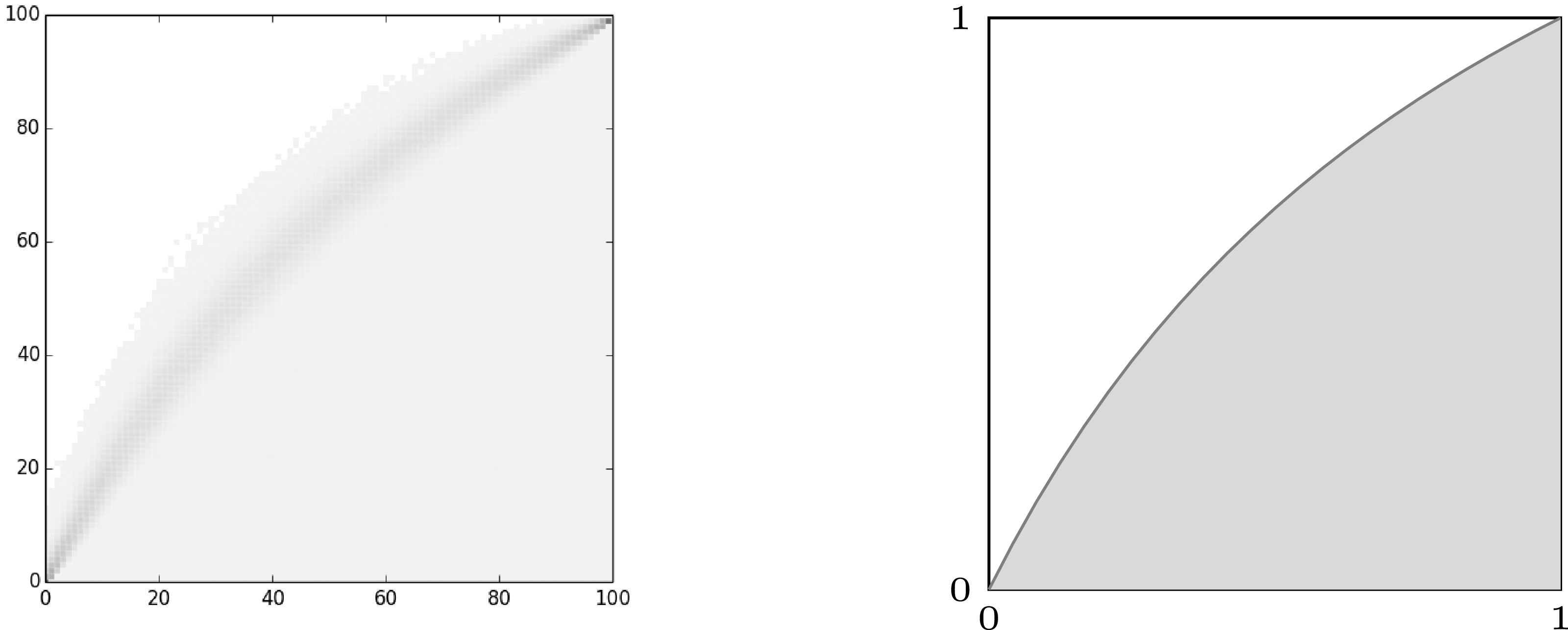
 10000
 n=100
 θ=λn
 λ=1
 (i,j)
 σ
 σ(i)=j
 x↦x(λ+1)λ+x
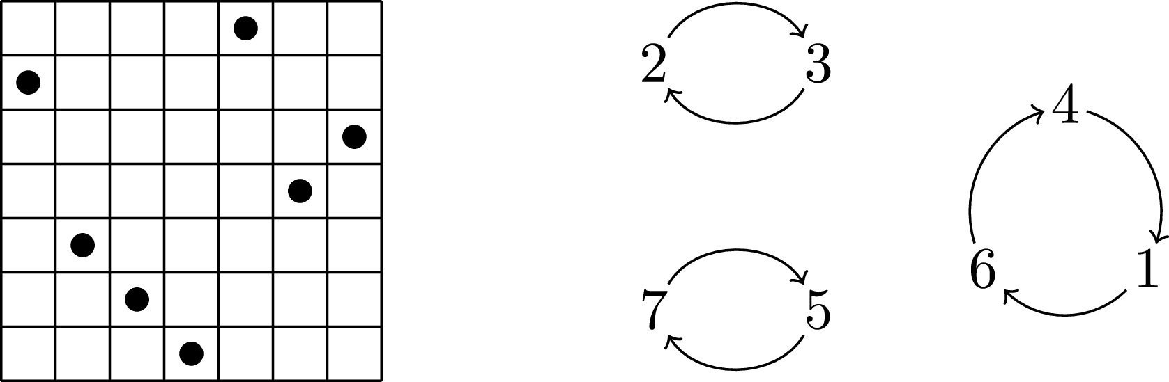
 τ=6321745
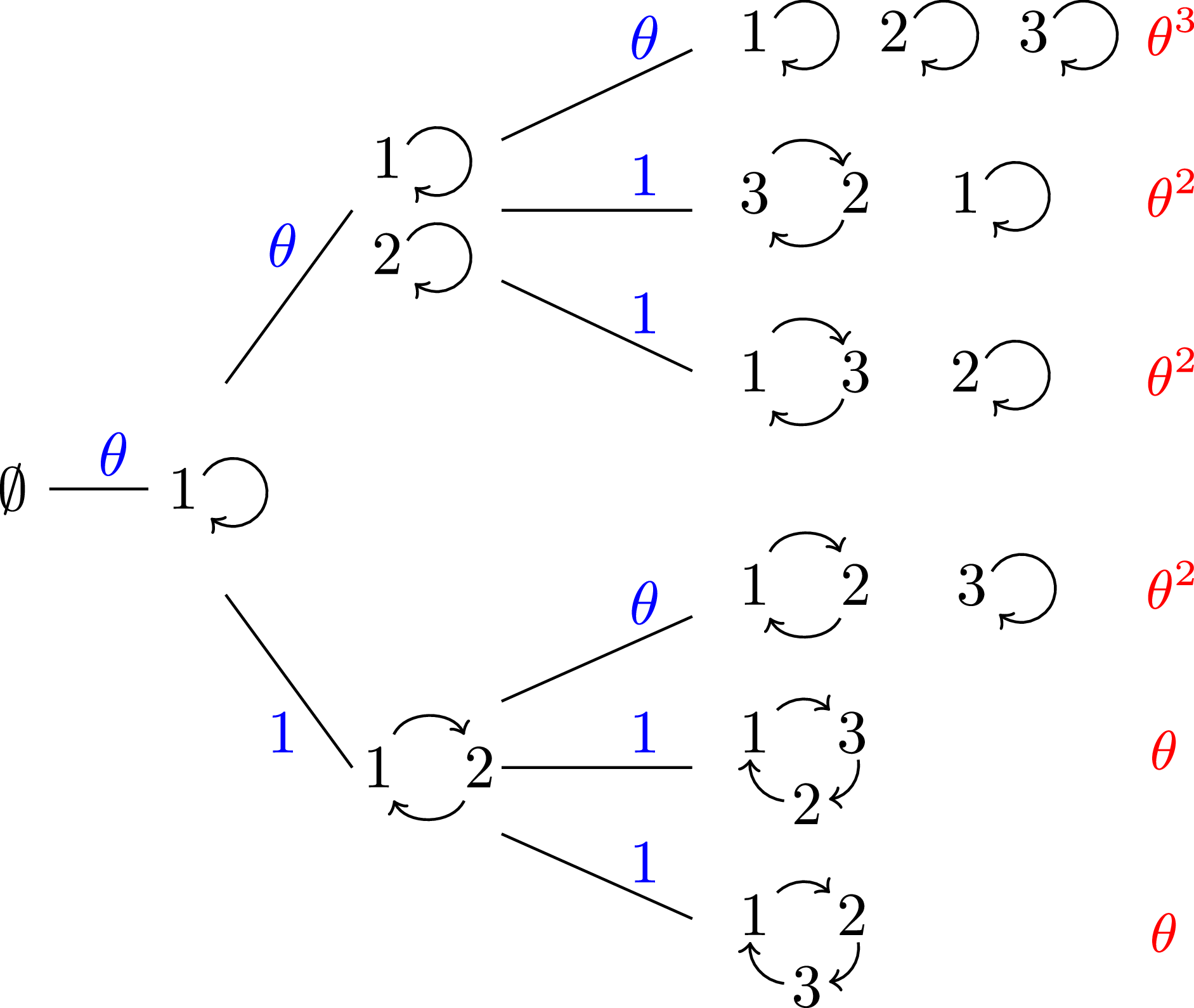
 S3
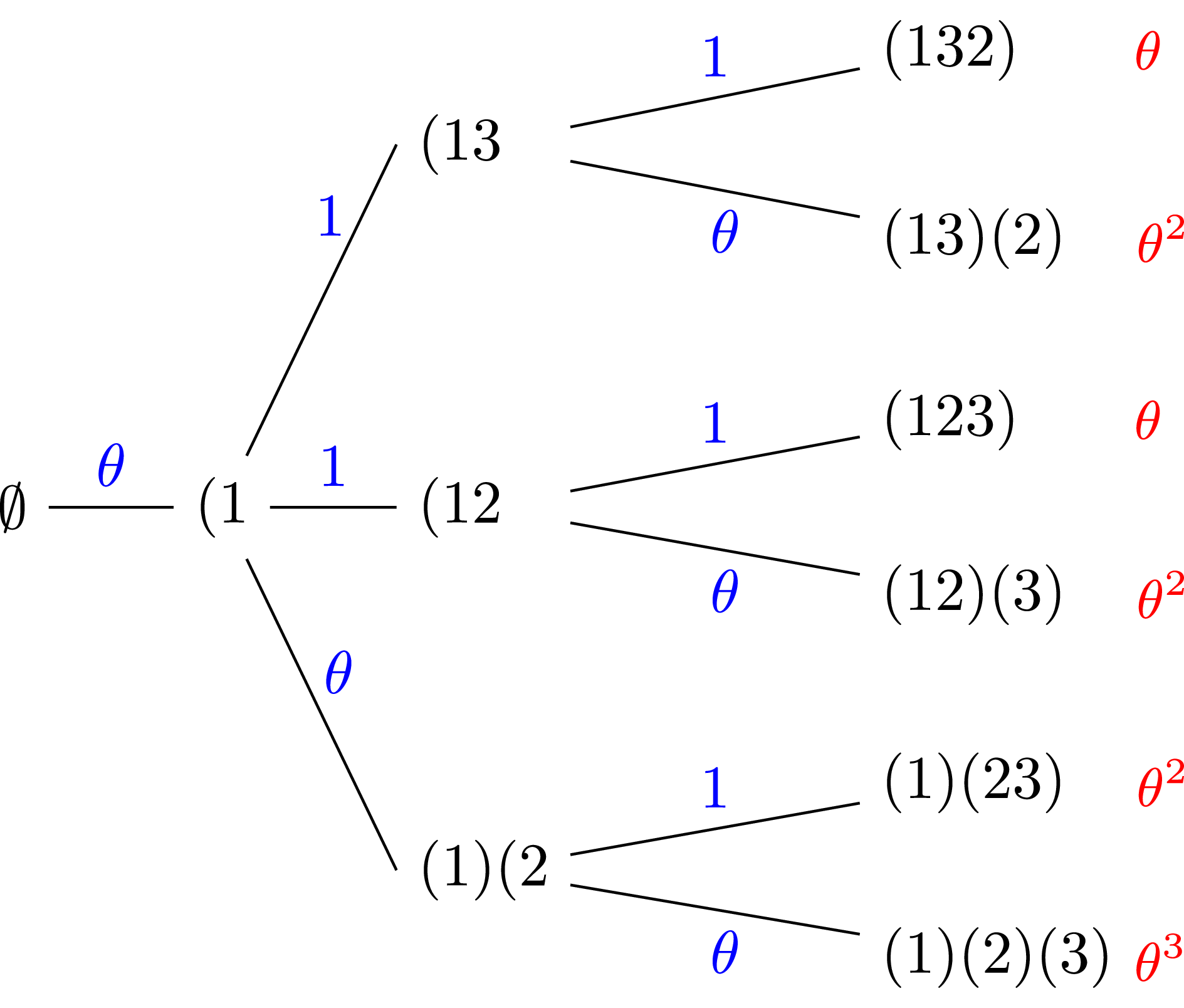
 S3
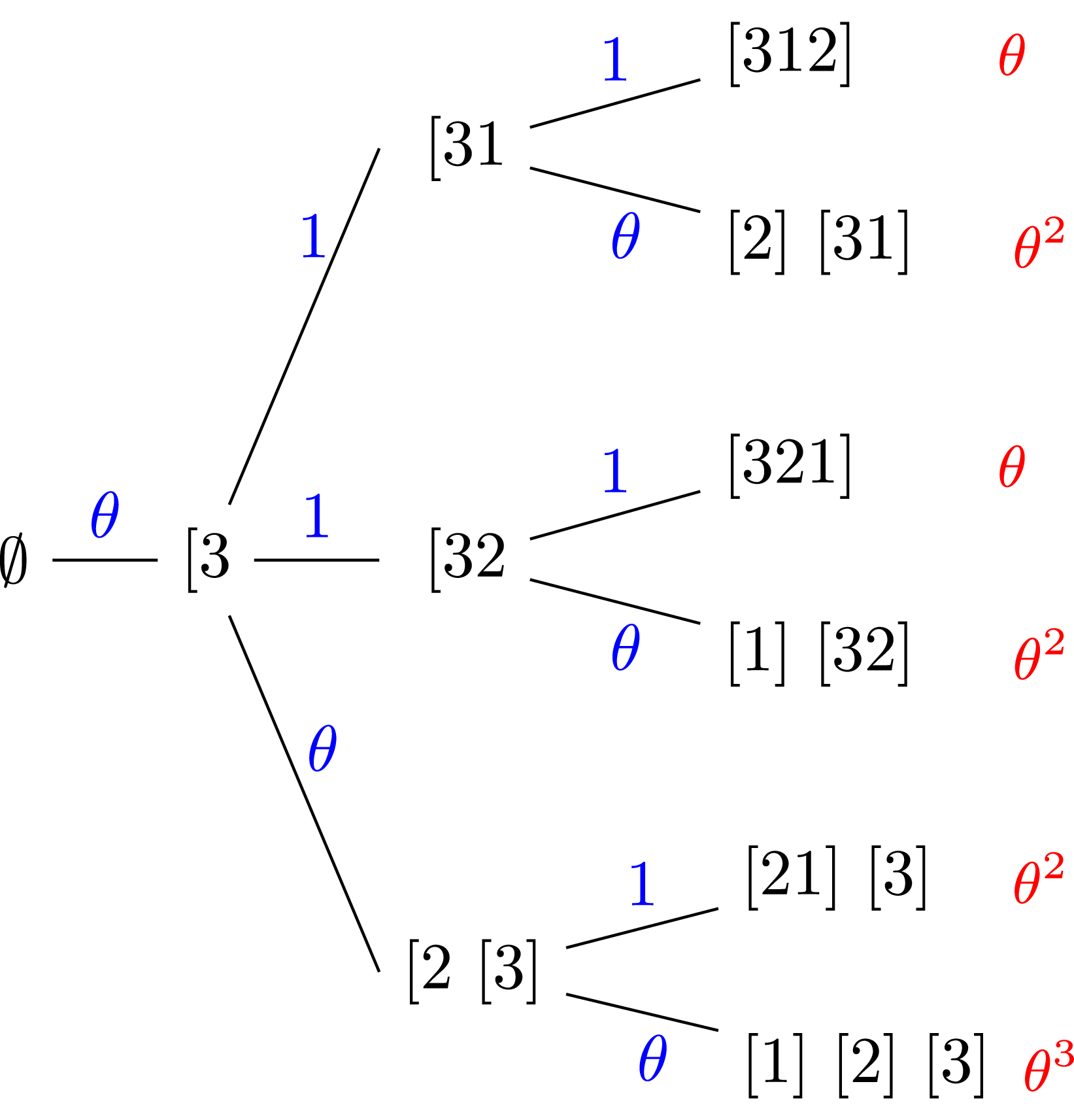
 S3
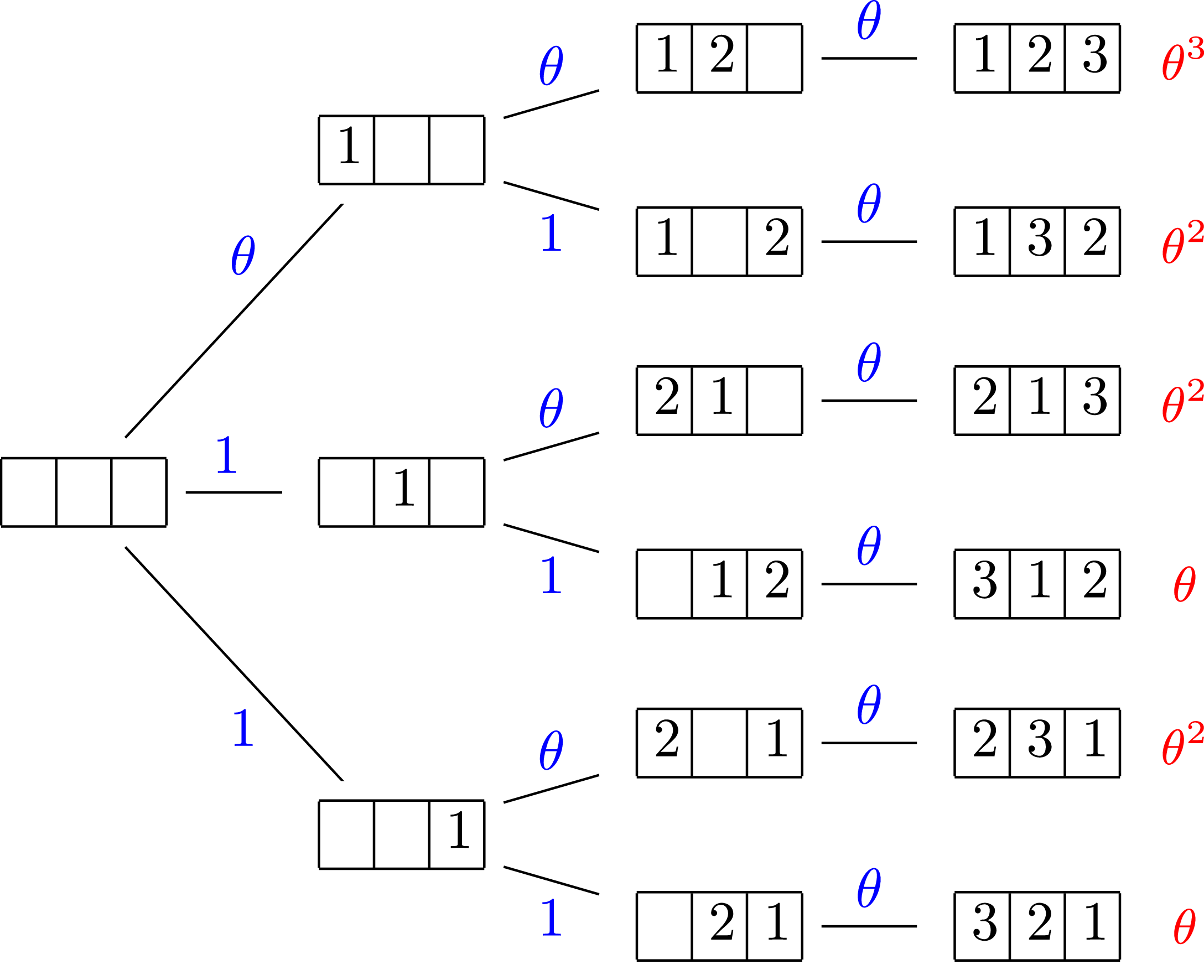
 S3
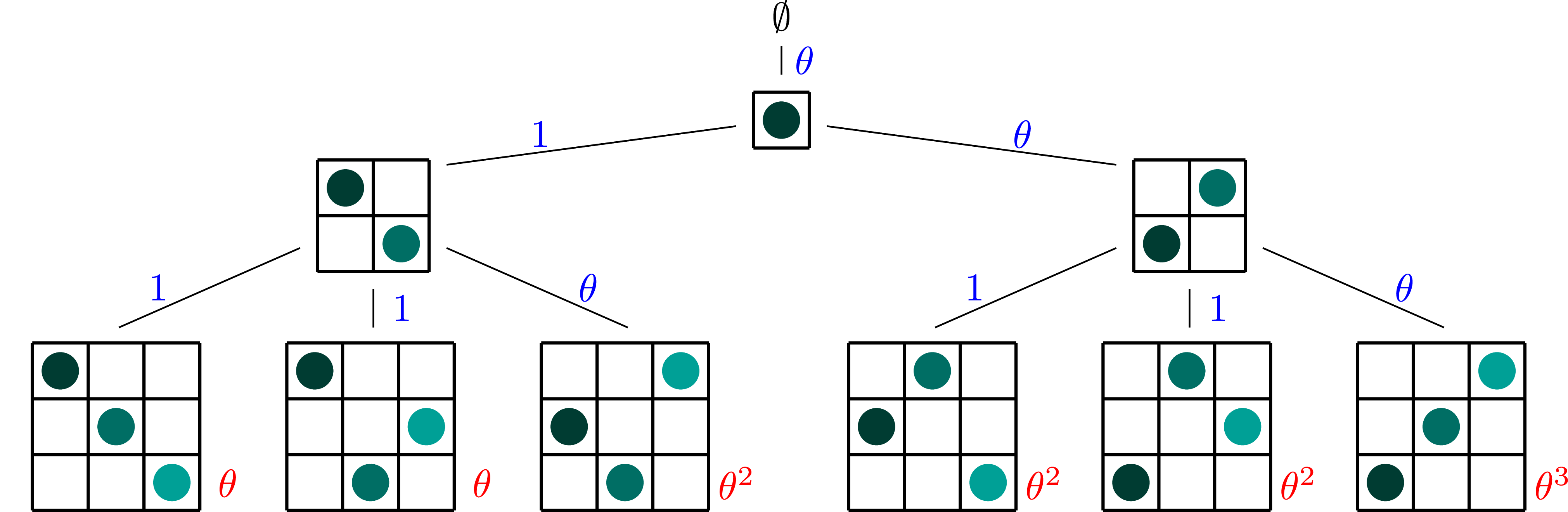
 S3
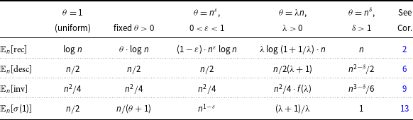
 θ
 f(λ)=1−2λ+2λ2log(1+1/λ)
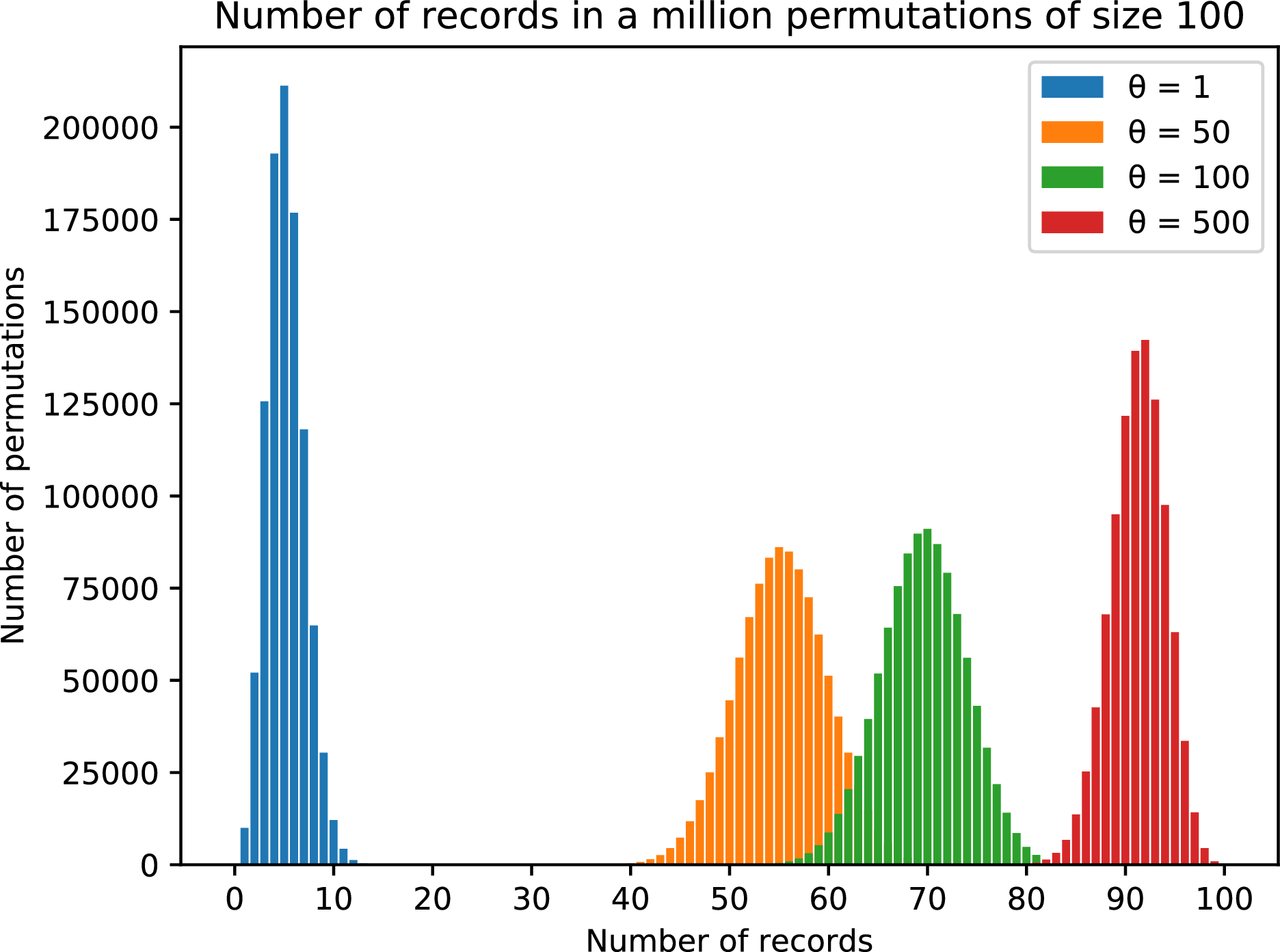
 106
 100
 θ
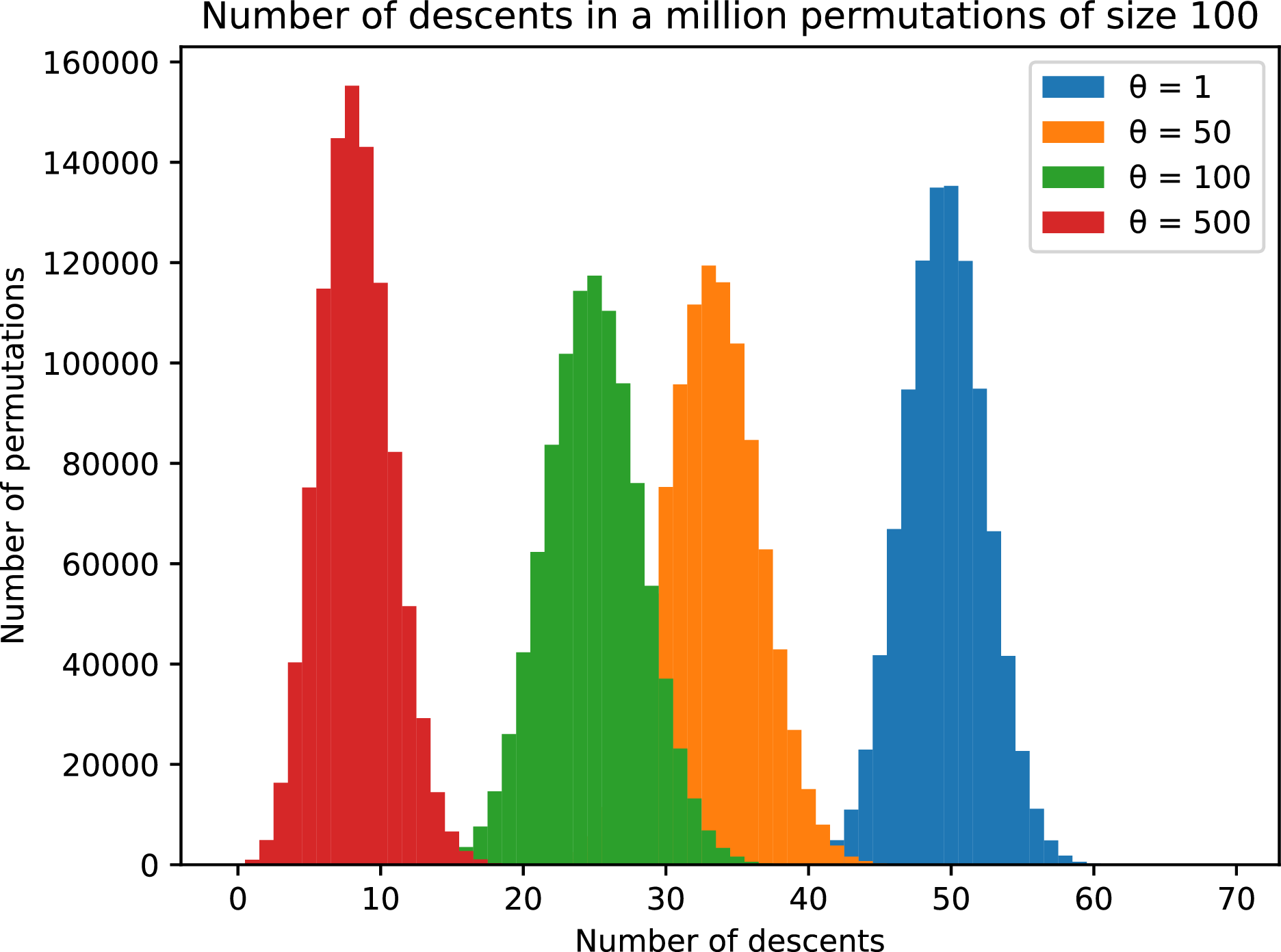
 106
 100
 θ
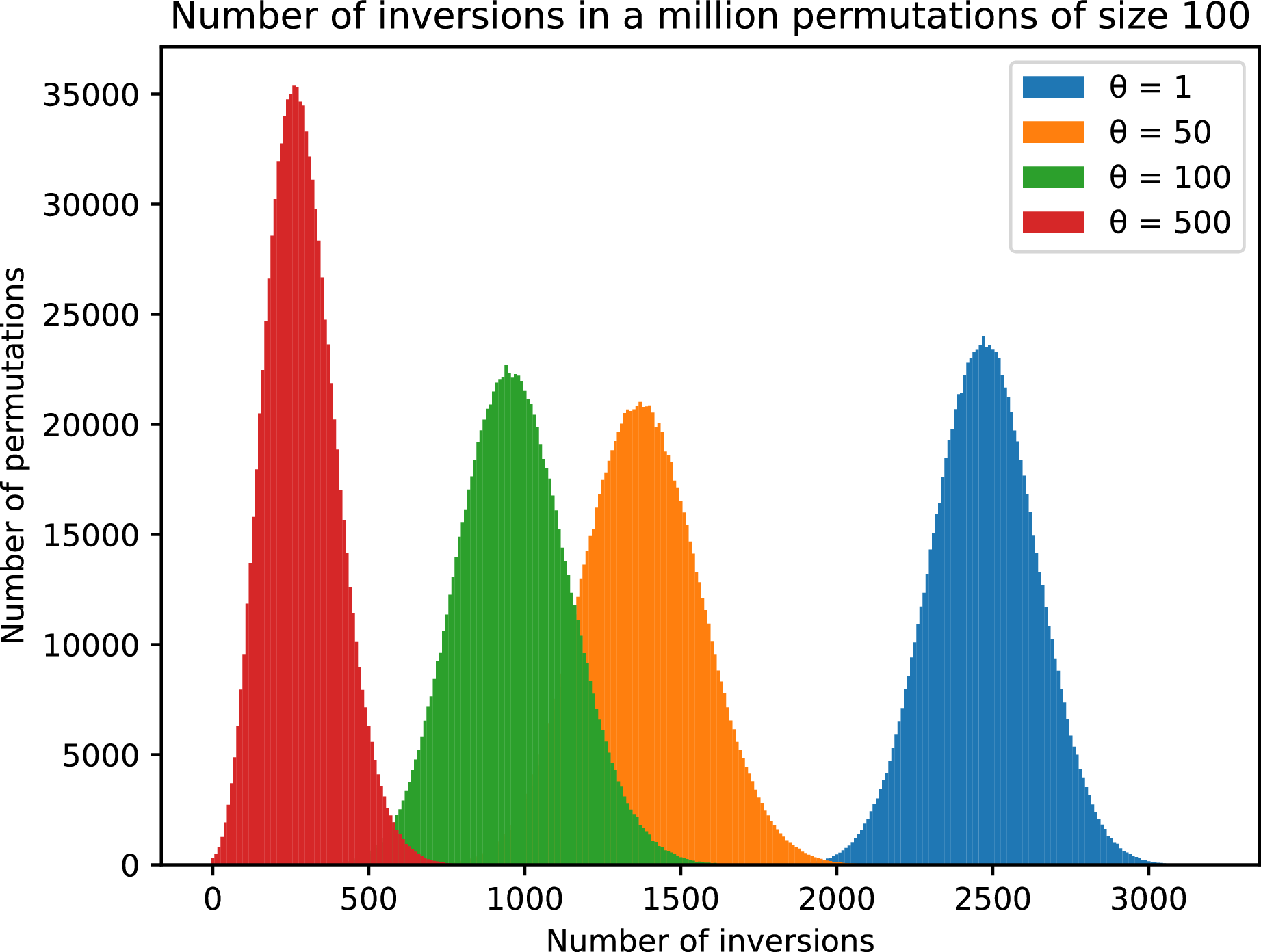
 106
 100
 θ
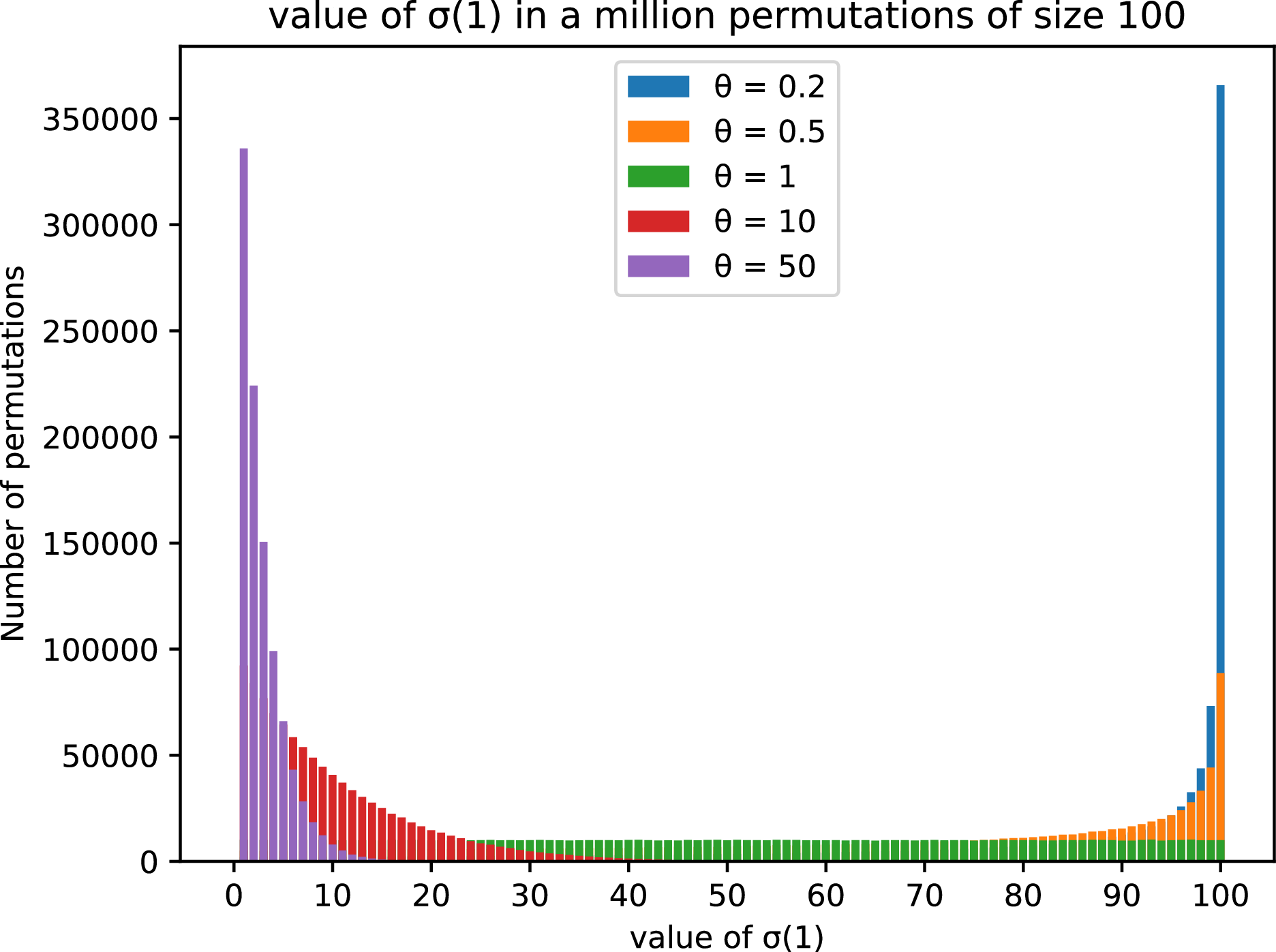
 σ(1)
 106
 100
 θ

 S100
 θ=1
 ,50,100,
 500
 (i,j)
 σ
 σ(i)=j
 100
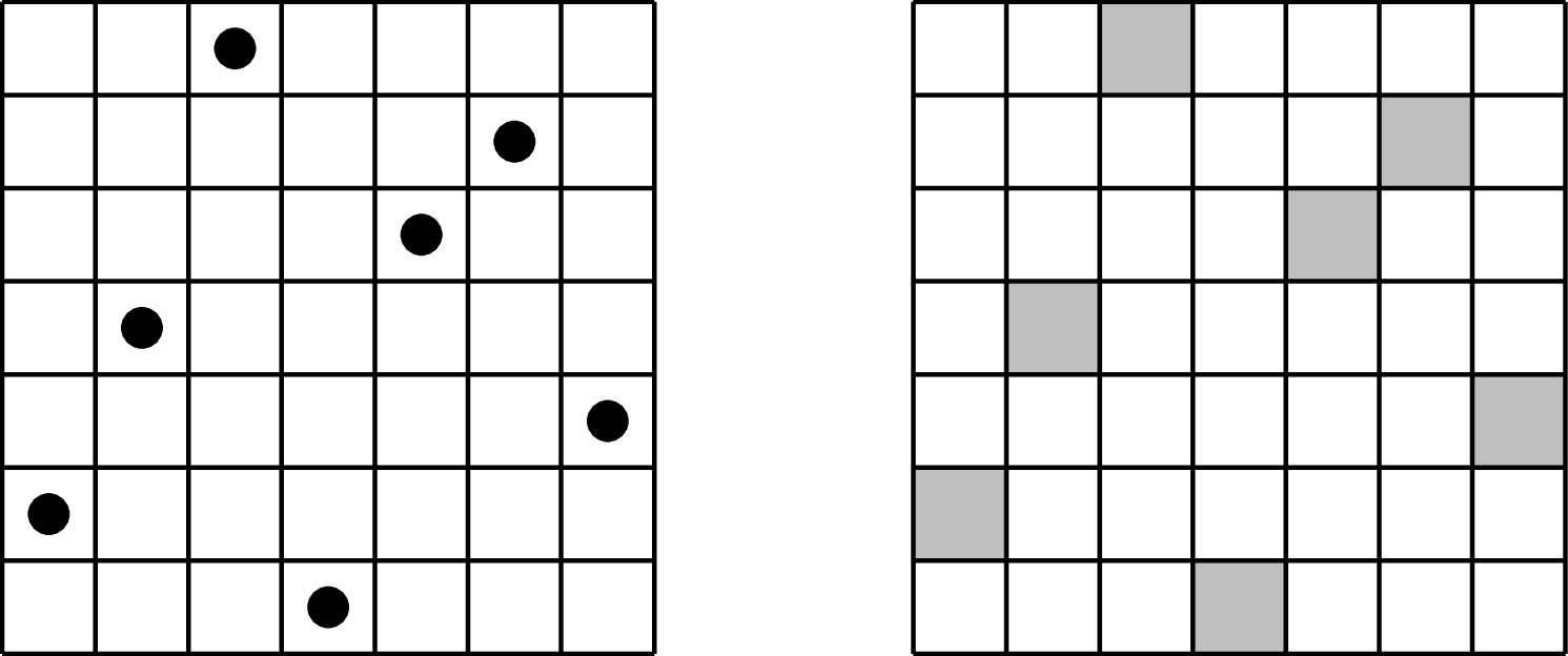
 σ=2471563
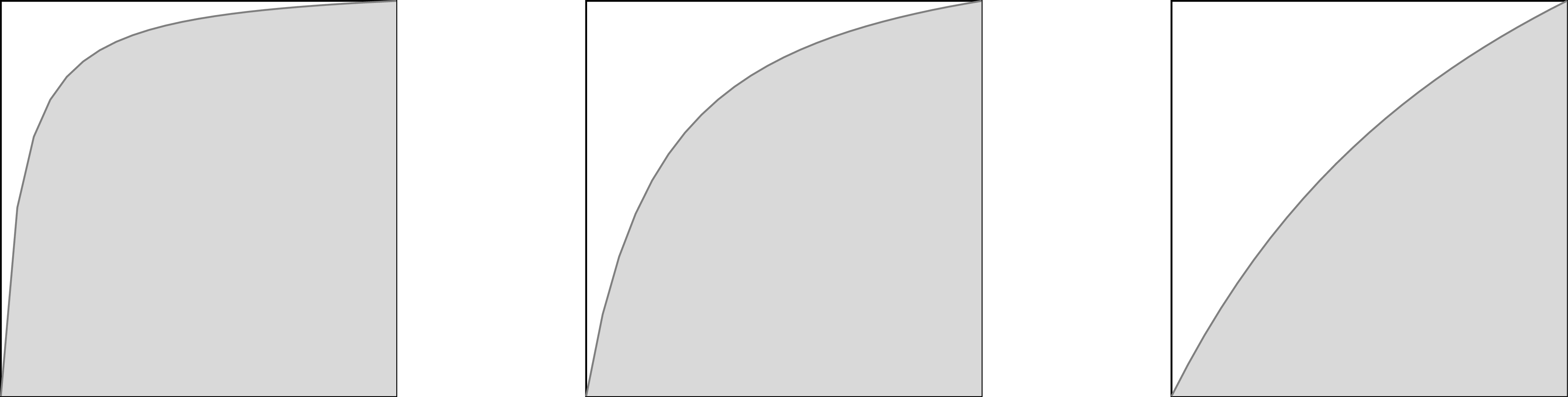
 μ
 λ=0.05
 0.2
 1
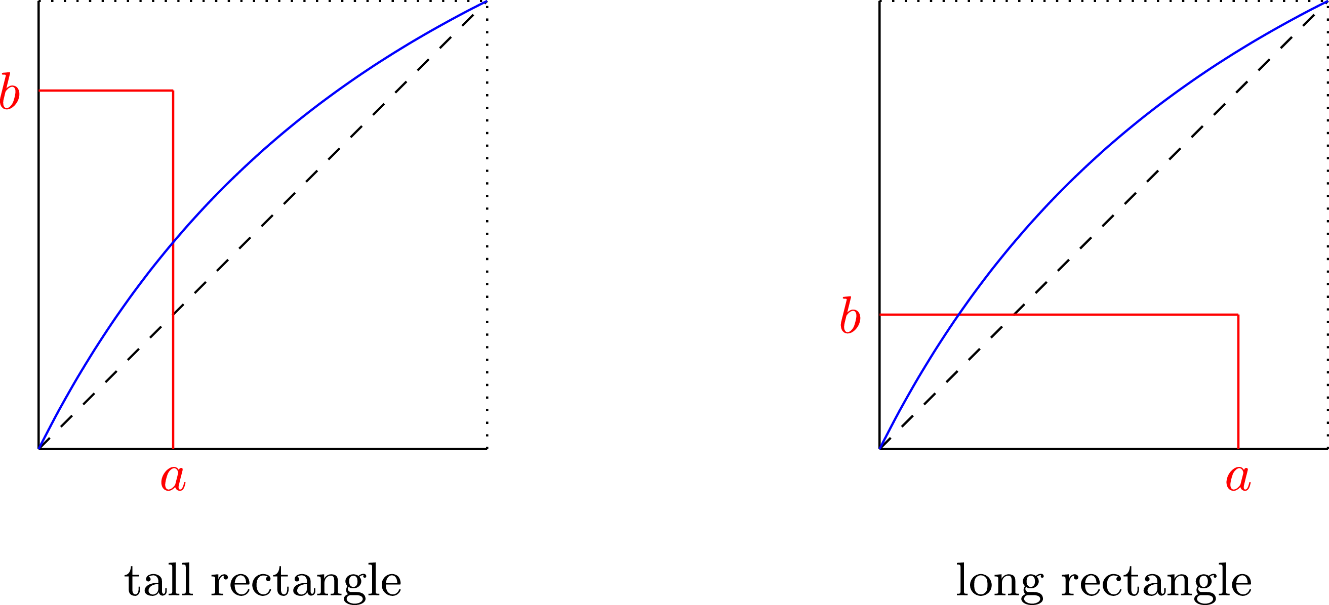
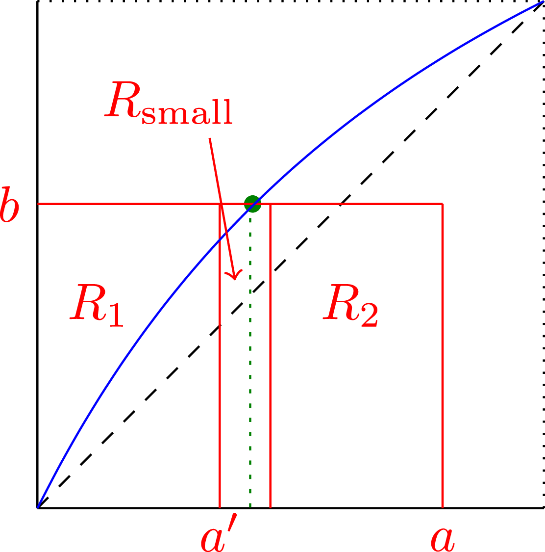
 R
 R1⊎Rsmall⊎R2


