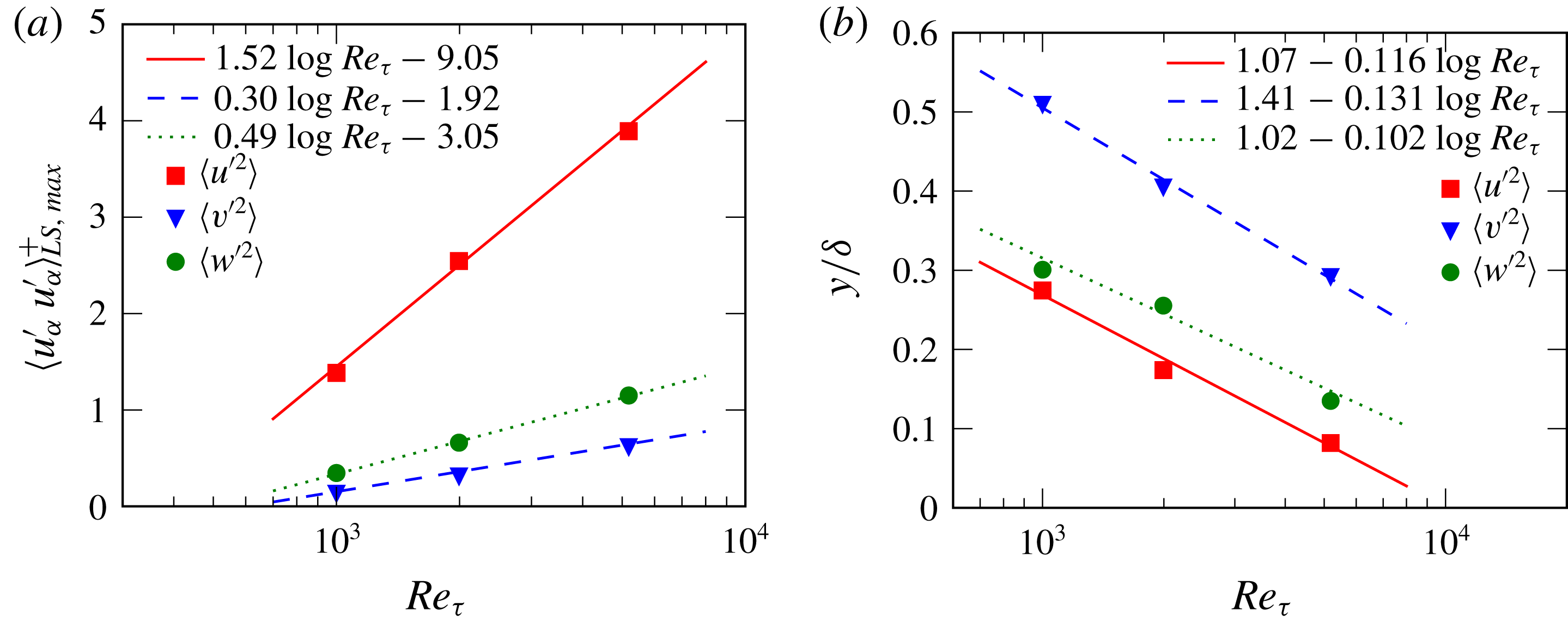
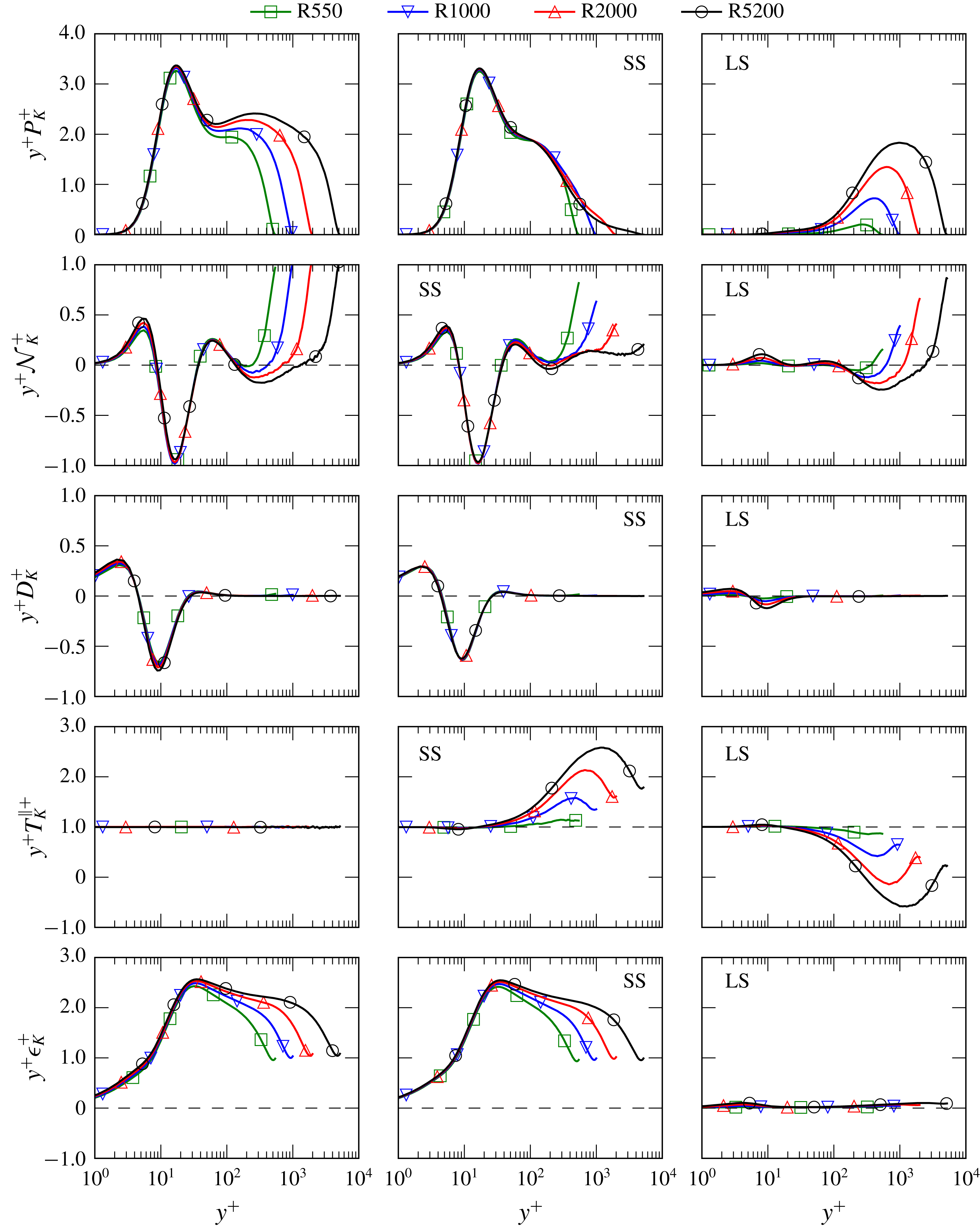
1 Introduction
High Reynolds number (
 $Re$
) wall-bounded turbulence is an important physical phenomenon, and has been challenging to study experimentally, computationally and theoretically. The presence of the wall causes strong anisotropy and inhomogeneity which invalidates the simple Kolmogorov description of turbulence. Also, the length and time scales of the turbulence near the wall get smaller, relative to outer scales, as
 $Re$
increases, which increases demands on instrumentation or computational resources in experimental or computations studies. However, the study of wall-bounded turbulence at high
 $Re$
has greatly advanced with the remarkable improvements in experimental techniques and computing power over the last few decades.
Perhaps the most important characteristic of wall-bounded turbulence at high
 $Re$
is the scale separation between the near wall and outer turbulence. Millikan (Reference Millikan1938) argued that the mean velocity profile in the overlap region has a logarithmic variation with wall-normal distance at infinitely high
 $Re$
. Even though his prediction is generally accepted, the universality of the von Kármán constant,
 $\unicode[STIX]{x1D705}$
, has remained controversial (Nagib & Chauhan Reference Nagib and Chauhan2008; Marusic et al.
Reference Marusic, McKeon, Monkewitz, Nagib, Smits and Sreenivasan2010c
; Monkewitz Reference Monkewitz2017; Luchini Reference Luchini2018). Nonetheless, the existence of a logarithmic mean velocity is an indication of the separation of scales, and has been observed in experimental and computational studies. The variance of the velocity components, or turbulent kinetic energy (TKE), also exhibits near-wall/outer scale separation. For example, Hutchins & Marusic (Reference Hutchins and Marusic2007b
) show that small scales dominate near the wall, while large scales dominate away from the wall. Further, the contribution of the large-scale outer turbulence is shown to grow with increasing
 $Re$
, causing the streamwise velocity variance to have both an inner-layer peak and an outer-layer peak (Fernholz & Finley Reference Fernholz and Finley1996; Morrison et al.
Reference Morrison, McKeon, Jiang and Smits2004). Moreover, based on his ‘attached’ eddy hypothesis, Townsend (Reference Townsend1976) predicted that, at high
 $Re$
and in the overlap region between inner and outer layers, the streamwise and spanwise velocity variances decrease logarithmically with wall-normal distance, and that the wall-normal variance and streamwise/wall-normal velocity covariance are constants. However, there is only limited experimental evidence (Marusic, Mathis & Hutchins Reference Marusic, Mathis and Hutchins2010a
; Hultmark et al.
Reference Hultmark, Vallikivi, Bailey and Smits2012) for the logarithmic variation of the streamwise variance at very high
 $Re$
(say
 $Re_{\unicode[STIX]{x1D70F}}\gtrsim 20\,000$
). Here,
 $Re_{\unicode[STIX]{x1D70F}}$
is the friction Reynolds number based on the friction velocity (
 $u_{\unicode[STIX]{x1D70F}}\equiv \sqrt{\unicode[STIX]{x1D70F}_{w}/\unicode[STIX]{x1D70C}}$
), the channel half-width (
 $\unicode[STIX]{x1D6FF}$
) and the kinematic viscosity (
 $\unicode[STIX]{x1D708}$
), where
 $\unicode[STIX]{x1D70F}_{w}$
and
 $\unicode[STIX]{x1D70C}$
are the mean wall shear stress and fluid density, respectively. Agreement with Townsend’s predictions for the spanwise velocity variance has been observed in direct numerical simulation (DNS) (Lee & Moser Reference Lee and Moser2015a
).
The dynamics of near-wall turbulence is relatively well understood, since it can be studied with flows at relatively low
 $Re$
. Streamwise vortices create streaks, which become unstable and wavy. In turn, the wavy streaks stretch the streamwise vorticity creating new streamwise vortices, and ultimately new streaks. This ‘autonomous’ or ‘self-sustaining’ cycle occurs at the small scales characteristic of the near wall, and is maintained independent of the outer-layer turbulence (Hamilton, Kim & Waleffe Reference Hamilton, Kim and Waleffe1995; Jeong et al.
Reference Jeong, Hussain, Schoppa and Kim1997; Jiménez & Pinelli Reference Jiménez and Pinelli1999; Schoppa & Hussain Reference Schoppa and Hussain2002). At small scales, energy is transferred away from the wall through a self-similar ejection mechanism (del Álamo et al.
Reference del Álamo, Jiménez, Zandonade and Moser2004, Reference del Álamo, Jiménez, Zandonade and Moser2006; Jiménez & Moser Reference Jiménez and Moser2007). Also, the large scales in the outer layer transfer energy to the near-wall region, leaving ‘footprints’ that are effectively large-scale modulations of the small-scale near-wall turbulence (Ganapathisubramani et al.
Reference Ganapathisubramani, Hutchins, Monty, Chung and Marusic2012). This modulation by the outer layer increases with
 $Re$
, so that the contributions of large scales in the near-wall region also increase with
 $Re$
(DeGraaff & Eaton Reference DeGraaff and Eaton2000; Hutchins & Marusic Reference Hutchins and Marusic2007a
; Marusic et al.
Reference Marusic, Mathis and Hutchins2010a
; Marusic, Mathis & Hutchins Reference Marusic, Mathis and Hutchins2010b
). Here, to better understand this interplay between the inner- and outer-layer turbulence at high Reynolds number, we seek to ‘map’ the exchange of energy in the wall-normal direction, in scale and among components.
Of the many methods of studying wall-bounded turbulence, we focus here on the Reynolds stress transport equations (RSTE). The RSTE provide detailed information regarding the life cycle of the turbulence, which includes production, transport and dissipation. However, there have only been a limited number of studies of the terms in the RSTE because their computation requires high-fidelity three-dimensional velocity fields. For example, in the case of incompressible channel flows, Mansour, Kim & Moin (Reference Mansour, Kim and Moin1988) first performed an analysis of terms in the RSTE using the data from the
 $Re_{\unicode[STIX]{x1D70F}}=180$
direct numerical simulation (DNS) of Kim, Moin & Moser (Reference Kim, Moin and Moser1987). Two decades later, Hoyas & Jiménez (Reference Hoyas and Jiménez2008) analysed the
 $Re$
dependences of the RSTE terms using DNS data from channel flow at up to
 $Re_{\unicode[STIX]{x1D70F}}=2003$
. Both these studies focused on the profiles of each RSTE term and their scalings.
More than fifty years ago, Lumley (Reference Lumley1964) suggested the analysis of spectral budget equations in wall-bounded turbulence. One of the objectives of such a study would be to analyse the nonlinear transfer of energy between scales, as characterised by the exchange of energy among Fourier modes. In the usual Kolmogorov picture of turbulence, the net transfer of energy is from large scales (low wavenumbers) to small scales (high wavenumbers). However, Lumley (Reference Lumley1964) conjectured that the energy will be transferred from small scales to large, as distance from the wall increases, a so-called ‘inverse energy transfer’. Thirty years later, Domaradzki et al. (Reference Domaradzki, Liu, Härtel and Kleiser1994) performed a spectral analysis of the RSTE using DNS data of channel flow at
 $Re_{\unicode[STIX]{x1D70F}}=210$
and observed inverse energy transfers from small to large scales. Later, Bolotnov et al. (Reference Bolotnov, Lahey, Drew, Jansen and Oberai2010) performed spectral analysis of RSTE at
 $Re_{\unicode[STIX]{x1D70F}}=180$
including viscous transport and dissipation terms. However Bolotnov et al. (Reference Bolotnov, Lahey, Drew, Jansen and Oberai2010) did not observe an inverse energy transfer. As will be seen in § 3.6, identifying inverse transfers from one-dimensional spectra can be misleading. Recently, Mizuno (Reference Mizuno2015, Reference Mizuno2016) performed RSTE spectral analysis using channel flow DNS data at up to
 $Re_{\unicode[STIX]{x1D70F}}=1000$
, and observed length scale dependences in the transport of TKE in the wall-normal direction. In parallel, Lee & Moser (Reference Lee and Moser2015b
) observed the same phenomena in DNS data up to
 $Re_{\unicode[STIX]{x1D70F}}=5200$
.
In noteworthy related studies: Richter (Reference Richter2015) performed a spectral analysis of the TKE budget equations using DNS of particle-laden turbulent plane Couette flows at up to
 $Re_{\unicode[STIX]{x1D70F}}=900$
to investigate the
 $Re$
and
 $St$
(Stokes number) dependences of the production and dissipation of TKE. Aulery et al. (Reference Aulery, Dupuy, Toutant, Bataille and Zhou2017) performed spectral analysis of the TKE budget in anisothermal turbulent channel flow up to
 $Re_{\unicode[STIX]{x1D70F}}=395$
, and also observed inverse energy transfers. Finally, Cimarelli, De Angelis & Casciola (Reference Cimarelli, De Angelis and Casciola2013), Cimarelli et al. (Reference Cimarelli, De Angelis, Schlatter, Brethouwer, Talamelli and Casciola2015, Reference Cimarelli, De Angelis, Jiménez and Casciola2016) studied the evolution equation of the second-order structure function as a function
 $(\boldsymbol{r},y)$
where
 $\boldsymbol{r}$
is the separation vector in the structure function and
 $y$
is the distance from the wall. They observed two distinct production mechanisms at different wall-normal distances and inverse energy transfers.
Up to now, most analysis of RSTE has been done in terms of TKE or the streamwise velocity variance, in relatively low
 $Re$
turbulence. The goal of this paper is to study the detailed flow of energy in the
 $y$
scale, and among velocity components in high Reynolds number turbulence. To pursue this, we use the DNS data of Lee & Moser (Reference Lee and Moser2015a
) at
 $Re_{\unicode[STIX]{x1D70F}}=5200$
, which exhibits many features of high
 $Re$
wall-bounded turbulent flows, such as logarithmic variation of the mean-velocity profiles and scale separations in the energy spectra. The remainder of this paper is organised as follows. Details of the analysis method, including the derivation of the spectral budget equation and visual representation of two-dimensional spectral densities in log-polar coordinates are provided in § 2. The spectral density of TKE components and their production, scale transfer, wall-normal transport and dissipation are explored in § 3 as functions of the wall-normal distance and scale. Finally, a summary and conclusions are provided in § 4.
2 Analysis details
In the following discussion, the velocity components in the streamwise (
 $x$
), wall-normal (
 $y$
) and spanwise (
 $z$
) directions are denoted as
 $u$
,
 $v$
and
 $w$
, respectively, and when using index notation, these directions are labelled 1, 2 and 3, respectively. The expected value is denoted with angle brackets (as in
 $\langle \cdot \rangle$
), and upper case
 $U$
and
 $P$
indicate the mean velocity and pressure, so that
 $\langle u_{i}\rangle =U_{i}$
. The velocity and pressure fluctuations are indicated with primes, e.g.
 $u_{i}=U_{i}+u_{i}^{\prime }$
, and as usual, a superscript ‘
 $+$
’ signifies non-dimensionalisation with the kinematic viscosity
 $\unicode[STIX]{x1D708}$
and the friction velocity
 $u_{\unicode[STIX]{x1D70F}}$
.
2.1 Simulation data
Direct numerical simulations of pressure-driven incompressible channel flows at different Reynolds numbers were performed (Lee & Moser Reference Lee and Moser2015a
), and the data from these simulations are used in the analysis reported here. The simulation parameters for each case are summarised in table 1. Note that in addition to the simulations reported in Lee & Moser (Reference Lee and Moser2015a
) a new simulation at
 $Re_{\unicode[STIX]{x1D70F}}\approx 2000$
was performed for completeness and consistency, and is also included here. In the direct numerical simulations, the wall-normal velocity–vorticity formulation of Kim et al. (Reference Kim, Moin and Moser1987) was used to solve the Navier–Stokes equations with Fourier–Galerkin discretisations in the
 $x$
and
 $z$
directions and a seventh-order b-spline representation in the
 $y$
direction. See Lee, Malaya & Moser (Reference Lee, Malaya and Moser2013), Lee et al. (Reference Lee, Ulerich, Malaya and Moser2014) and Lee & Moser (Reference Lee and Moser2015a
) for more details on the simulations and the numerical methods.
Summary of simulation parameters:
 $\unicode[STIX]{x0394}x$
and
 $\unicode[STIX]{x0394}z$
are in terms of Fourier modes for spectral methods;
 $\unicode[STIX]{x0394}y_{w}$
and
 $\unicode[STIX]{x0394}y_{c}$
are the b-spline knot spacings at the wall and the centre of the channel, respectively.
 $\unicode[STIX]{x1D6FF}$
– channel half-width,
 $Re_{\unicode[STIX]{x1D70F}}=u_{\unicode[STIX]{x1D70F}}\unicode[STIX]{x1D6FF}/\unicode[STIX]{x1D708}$
,
 $Tu_{\unicode[STIX]{x1D70F}}/\unicode[STIX]{x1D6FF}$
– total simulation time without transition. In all cases, the domain size in the
 $x$
and
 $z$
directions is
 $8\unicode[STIX]{x03C0}\unicode[STIX]{x1D6FF}$
and
 $3\unicode[STIX]{x03C0}\unicode[STIX]{x1D6FF}$
respectively.

2.2 Mathematical formulations
In this section, evolution equations for velocity spectral densities are derived. Equations for the velocity fluctuation are obtained by introducing the Reynolds decomposition in to the Navier–Stokes equations and are given by
 $$\begin{eqnarray}\frac{\unicode[STIX]{x2202}u_{i}^{\prime }}{\unicode[STIX]{x2202}t}=-U_{k}\frac{\unicode[STIX]{x2202}u_{i}^{\prime }}{\unicode[STIX]{x2202}x_{k}}-u_{k}^{\prime }\frac{\unicode[STIX]{x2202}U_{i}}{\unicode[STIX]{x2202}x_{k}}-\frac{\unicode[STIX]{x2202}u_{k}^{\prime }u_{i}^{\prime }}{\unicode[STIX]{x2202}x_{k}}+\frac{\unicode[STIX]{x2202}\overline{u_{k}^{\prime }u_{i}^{\prime }}}{\unicode[STIX]{x2202}x_{k}}-\frac{1}{\unicode[STIX]{x1D70C}}\frac{\unicode[STIX]{x2202}p^{\prime }}{\unicode[STIX]{x2202}x_{i}}+\unicode[STIX]{x1D708}\frac{\unicode[STIX]{x2202}^{2}u_{i}^{\prime }}{\unicode[STIX]{x2202}x_{k}\unicode[STIX]{x2202}x_{k}}.\end{eqnarray}$$
Consider two points separated from each other in only the horizontal directions, with coordinates
 $\boldsymbol{x}$
and
 $\tilde{\boldsymbol{x}}$
, where
 $y={\tilde{y}}$
. Also, let
 $r_{x}=\tilde{x}-x$
and
 $r_{z}=\tilde{z}-z$
be the separation between the points in the streamwise and spanwise directions. Further, let the velocities at the points
 $\boldsymbol{x}$
and
 $\tilde{\boldsymbol{x}}$
be
 $\boldsymbol{u}$
and
 $\tilde{\boldsymbol{u}}$
, respectively. The evolution equation for the two-point correlation tensor
 $\unicode[STIX]{x1D619}_{ij}=\langle u_{i}\tilde{u} _{j}\rangle$
can then be obtained from (2.1) as
 $$\begin{eqnarray}\displaystyle \frac{\unicode[STIX]{x2202}\unicode[STIX]{x1D619}_{ij}}{\unicode[STIX]{x2202}t}(r_{x},y,r_{z}) & = & \displaystyle \left\langle u_{i}^{\prime }\frac{\unicode[STIX]{x2202}\tilde{u} _{j}^{\prime }}{\unicode[STIX]{x2202}t}+\tilde{u} _{j}^{\prime }\frac{\unicode[STIX]{x2202}u_{i}^{\prime }}{\unicode[STIX]{x2202}t}\right\rangle \nonumber\\ \displaystyle & = & \displaystyle \underbrace{-\langle \tilde{u} _{j}^{\prime }u_{k}^{\prime }\rangle \frac{\unicode[STIX]{x2202}U_{i}}{\unicode[STIX]{x2202}x_{k}}-\langle u_{i}^{\prime }\tilde{u} _{k}^{\prime }\rangle \frac{\unicode[STIX]{x2202}U_{j}}{\unicode[STIX]{x2202}\tilde{x}_{k}}}_{\displaystyle \unicode[STIX]{x1D619}_{ij}^{P}}\;\;\underbrace{-\left\langle \tilde{u} _{j}^{\prime }\frac{\unicode[STIX]{x2202}u_{k}^{\prime }u_{i}^{\prime }}{\unicode[STIX]{x2202}x_{k}}+u_{i}^{\prime }\frac{\unicode[STIX]{x2202}\tilde{u} _{k}^{\prime }\tilde{u} _{j}^{\prime }}{\unicode[STIX]{x2202}\tilde{x}_{k}}\right\rangle }_{\displaystyle \unicode[STIX]{x1D619}_{ij}^{T}}\nonumber\\ \displaystyle & & \displaystyle \underbrace{-\frac{1}{\unicode[STIX]{x1D70C}}\left\langle \tilde{u} _{j}^{\prime }\frac{\unicode[STIX]{x2202}p^{\prime }}{\unicode[STIX]{x2202}x_{i}}+u_{i}^{\prime }\frac{\unicode[STIX]{x2202}\tilde{p}^{\prime }}{\unicode[STIX]{x2202}\tilde{x}_{j}}\right\rangle }_{\displaystyle \unicode[STIX]{x1D619}_{ij}^{\unicode[STIX]{x1D6F1}}}\;\;+\underbrace{\unicode[STIX]{x1D708}\left\langle \tilde{u} _{j}^{\prime }\frac{\unicode[STIX]{x2202}^{2}u_{i}^{\prime }}{\unicode[STIX]{x2202}x_{k}\unicode[STIX]{x2202}x_{k}}+u_{i}^{\prime }\frac{\unicode[STIX]{x2202}^{2}\tilde{u} _{j}^{\prime }}{\unicode[STIX]{x2202}\tilde{x}_{k}\unicode[STIX]{x2202}\tilde{x}_{k}}\right\rangle }_{\displaystyle \unicode[STIX]{x1D619}_{ij}^{\unicode[STIX]{x1D708}}},\end{eqnarray}$$
where the terms labelled
 $\unicode[STIX]{x1D619}_{ij}^{P}$
,
 $\unicode[STIX]{x1D619}_{ij}^{T}$
,
 $\unicode[STIX]{x1D619}_{ij}^{\unicode[STIX]{x1D6F1}}$
and
 $\unicode[STIX]{x1D619}_{ij}^{\unicode[STIX]{x1D708}}$
are interpreted as production, turbulent convection, pressure and viscous terms, respectively. Terms in (2.2) are functions of only
 $r_{x}$
,
 $y$
and
 $r_{z}$
due to the homogeneity in the horizontal (
 $x$
and
 $z$
) directions. Note that the Reynolds stress transport equation, also known as the budget equation for
 $\langle u_{i}^{\prime }u_{j}^{\prime }\rangle$
, is a special case of (2.2) where
 $r_{x}=r_{z}=0$
. Equation (2.2) can be simplified by taking advantage of the following relationships, where
 $\unicode[STIX]{x1D6FC}$
signifies an index for one of the wall-parallel directions (i.e. 1 or 3):
 $$\begin{eqnarray}\displaystyle & \displaystyle \frac{\unicode[STIX]{x2202}u_{i}}{\unicode[STIX]{x2202}\tilde{x}_{\unicode[STIX]{x1D6FC}}}=\frac{\unicode[STIX]{x2202}\tilde{u} _{j}}{\unicode[STIX]{x2202}x_{\unicode[STIX]{x1D6FC}}}=0, & \displaystyle\end{eqnarray}$$
 $$\begin{eqnarray}\displaystyle & \displaystyle \frac{\unicode[STIX]{x2202}U}{\unicode[STIX]{x2202}x_{\unicode[STIX]{x1D6FC}}}=\frac{\unicode[STIX]{x2202}U}{\unicode[STIX]{x2202}\tilde{x}_{\unicode[STIX]{x1D6FC}}}=0, & \displaystyle\end{eqnarray}$$
 $$\begin{eqnarray}\displaystyle & \displaystyle V=W=0, & \displaystyle\end{eqnarray}$$
 $$\begin{eqnarray}\displaystyle & \displaystyle y={\tilde{y}}, & \displaystyle\end{eqnarray}$$
 $$\begin{eqnarray}\displaystyle & \displaystyle \left.\frac{\unicode[STIX]{x2202}}{\unicode[STIX]{x2202}\tilde{x}_{\unicode[STIX]{x1D6FC}}}\right|_{x_{\unicode[STIX]{x1D6FC}}}=-\left.\frac{\unicode[STIX]{x2202}}{\unicode[STIX]{x2202}x_{\unicode[STIX]{x1D6FC}}}\right|_{\tilde{x}_{\unicode[STIX]{x1D6FC}}}=\frac{\unicode[STIX]{x2202}}{\unicode[STIX]{x2202}r_{\unicode[STIX]{x1D6FC}}}. & \displaystyle\end{eqnarray}$$
The
 $\unicode[STIX]{x1D619}_{ij}^{P}$
term is interpreted as production because it arises from the interaction between the fluctuations and the mean-velocity gradient and results in a net transfer of energy from the mean to the turbulent fluctuations. Since only the streamwise component of the mean velocity is non-zero, and because it varies only in the wall-normal direction,
 $\unicode[STIX]{x1D619}_{ij}^{P}$
can be written
 $$\begin{eqnarray}\unicode[STIX]{x1D619}_{ij}^{P}=-(\langle \tilde{u} _{j}^{\prime }v^{\prime }\rangle \unicode[STIX]{x1D6FF}_{1i}+\langle u_{i}^{\prime }\tilde{v}^{\prime }\rangle \unicode[STIX]{x1D6FF}_{1j})\frac{\unicode[STIX]{x2202}U}{\unicode[STIX]{x2202}y}.\end{eqnarray}$$
Further, for zero separation, symmetry requires that
 $\unicode[STIX]{x1D619}_{13}^{P}=\unicode[STIX]{x1D619}_{31}^{P}=0$
, leaving non-zero production of only the streamwise velocity variance and the Reynolds shear stress, as is well known.
To facilitate the interpretation of the DNS data, it will also be useful to decompose the
 $\unicode[STIX]{x1D619}_{ij}^{T}$
,
 $\unicode[STIX]{x1D619}_{ij}^{\unicode[STIX]{x1D6F1}}$
and
 $\unicode[STIX]{x1D619}_{ij}^{\unicode[STIX]{x1D708}}$
terms, so that different effects can be isolated. In general, such decompositions are not unique (Lumley Reference Lumley1975), but we select the following decompositions of
 $\unicode[STIX]{x1D619}_{ij}^{T}$
,
 $\unicode[STIX]{x1D619}_{ij}^{\unicode[STIX]{x1D6F1}}$
and
 $\unicode[STIX]{x1D619}_{ij}^{\unicode[STIX]{x1D708}}$
, because they are consistent with the definitions used by Mansour et al. (Reference Mansour, Kim and Moin1988) and many others for the Reynolds stress transport equations when
 $r_{x}$
and
 $r_{z}$
approach zero.
First, the turbulent term
 $\unicode[STIX]{x1D619}_{ij}^{T}$
can be decomposed into two terms as follows:
 $$\begin{eqnarray}\unicode[STIX]{x1D619}_{ij}^{T}=\unicode[STIX]{x1D619}_{ij}^{T^{\bot }}+\unicode[STIX]{x1D619}_{ij}^{T^{\Vert }},\end{eqnarray}$$
where
 $\unicode[STIX]{x1D619}_{ij}^{T^{\bot }}$
and
 $\unicode[STIX]{x1D619}_{ij}^{T^{\Vert }}$
satisfy
 $$\begin{eqnarray}\displaystyle & \displaystyle \int _{0}^{\unicode[STIX]{x1D6FF}}\unicode[STIX]{x1D619}_{ij}^{T^{\bot }}\,\text{d}y=0,\quad \forall \;(r_{x},r_{z}), & \displaystyle\end{eqnarray}$$
 $$\begin{eqnarray}\displaystyle & \displaystyle \lim _{\substack{ r_{x}\rightarrow 0 \\ r_{z}\rightarrow 0}}\displaystyle \unicode[STIX]{x1D619}_{ij}^{T^{\Vert }}=0,\quad \forall \;y. & \displaystyle\end{eqnarray}$$
These conditions allow
 $\unicode[STIX]{x1D619}_{ij}^{T^{\bot }}$
to be interpreted as the transport of the two-point correlation in the wall-normal direction and
 $\unicode[STIX]{x1D619}_{ij}^{T^{\Vert }}$
to be interpreted as the transfer across scales. The decomposition that satisfies (2.6) and (2.7), and is consistent with the definitions of Mansour et al. (Reference Mansour, Kim and Moin1988) and Mizuno (Reference Mizuno2016), is
 $$\begin{eqnarray}\unicode[STIX]{x1D619}_{ij}^{T^{\bot }}=-\frac{1}{2}\left(\frac{\unicode[STIX]{x2202}\langle \tilde{u} _{j}^{\prime }u_{i}^{\prime }v^{\prime }\rangle }{\unicode[STIX]{x2202}y}+\frac{\unicode[STIX]{x2202}\langle u_{i}^{\prime }\tilde{u} _{j}^{\prime }\tilde{v}^{\prime }\rangle }{\unicode[STIX]{x2202}y}\right)\end{eqnarray}$$
and
 $$\begin{eqnarray}\displaystyle \unicode[STIX]{x1D619}_{ij}^{T^{\Vert }} & = & \displaystyle \frac{\unicode[STIX]{x2202}\langle \tilde{u} _{j}^{\prime }u_{i}^{\prime }u^{\prime }\rangle }{\unicode[STIX]{x2202}r_{x}}-\frac{\unicode[STIX]{x2202}\langle u_{i}^{\prime }\tilde{u} _{j}^{\prime }\tilde{u} ^{\prime }\rangle }{\unicode[STIX]{x2202}r_{x}}+\frac{\unicode[STIX]{x2202}\langle \tilde{u} _{j}^{\prime }u_{i}^{\prime }w^{\prime }\rangle }{\unicode[STIX]{x2202}r_{z}}-\frac{\unicode[STIX]{x2202}\langle u_{i}^{\prime }\tilde{u} _{j}^{\prime }\tilde{w}^{\prime }\rangle }{\unicode[STIX]{x2202}r_{z}}\nonumber\\ \displaystyle & & \displaystyle -\,\frac{1}{2}\left(\frac{\unicode[STIX]{x2202}\langle \tilde{u} _{j}^{\prime }u_{i}^{\prime }v^{\prime }\rangle }{\unicode[STIX]{x2202}y}+\frac{\unicode[STIX]{x2202}\langle u_{i}^{\prime }\tilde{u} _{j}^{\prime }\tilde{v}^{\prime }\rangle }{\unicode[STIX]{x2202}y}\right)+\left\langle u_{i}^{\prime }v^{\prime }\frac{\unicode[STIX]{x2202}\tilde{u} _{j}^{\prime }}{\unicode[STIX]{x2202}y}\right\rangle +\left\langle \tilde{u} _{j}^{\prime }\tilde{v}^{\prime }\frac{\unicode[STIX]{x2202}u_{i}^{\prime }}{\unicode[STIX]{x2202}y}\right\rangle .\end{eqnarray}$$
The pressure term
 $\unicode[STIX]{x1D619}_{ij}^{\unicode[STIX]{x1D6F1}}$
is decomposed into two terms
 $$\begin{eqnarray}\unicode[STIX]{x1D619}_{ij}^{\unicode[STIX]{x1D6F1}}=-\frac{1}{\unicode[STIX]{x1D70C}}\left\langle \tilde{u} _{j}^{\prime }\frac{\unicode[STIX]{x2202}p^{\prime }}{\unicode[STIX]{x2202}x_{i}}+u_{i}^{\prime }\frac{\unicode[STIX]{x2202}\tilde{p}^{\prime }}{\unicode[STIX]{x2202}\tilde{x}_{j}}\right\rangle =\unicode[STIX]{x1D619}_{ij}^{\unicode[STIX]{x1D6F1}^{d}}+\unicode[STIX]{x1D619}_{ij}^{\unicode[STIX]{x1D6F1}^{s}},\end{eqnarray}$$
where
 $\unicode[STIX]{x1D619}_{ij}^{\unicode[STIX]{x1D6F1}^{d}}$
and
 $\unicode[STIX]{x1D619}_{ij}^{\unicode[STIX]{x1D6F1}^{s}}$
satisfy:
 $$\begin{eqnarray}\displaystyle & \displaystyle \int _{0}^{\unicode[STIX]{x1D6FF}}\unicode[STIX]{x1D619}_{ij}^{\unicode[STIX]{x1D6F1}^{d}}\,\text{d}y=0,\quad \forall \;(r_{x},r_{z}), & \displaystyle\end{eqnarray}$$
 $$\begin{eqnarray}\displaystyle & \displaystyle \unicode[STIX]{x1D619}_{ii}^{\unicode[STIX]{x1D6F1}^{s}}=0,\quad \forall \;(r_{x},y,r_{z}). & \displaystyle\end{eqnarray}$$
These conditions allow
 $\unicode[STIX]{x1D619}_{ij}^{\unicode[STIX]{x1D6F1}^{d}}$
to be interpreted as pressure transport of the two-point correlation in the
 $y$
direction, and
 $\unicode[STIX]{x1D619}_{ij}^{\unicode[STIX]{x1D6F1}^{s}}$
as the energy exchange between velocity components. The decomposition is chosen to be
 $$\begin{eqnarray}\displaystyle & \displaystyle \unicode[STIX]{x1D619}_{ij}^{\unicode[STIX]{x1D6F1}^{d}}=\frac{1}{\unicode[STIX]{x1D70C}}\left(\frac{\unicode[STIX]{x2202}\langle \tilde{u} _{j}p\rangle }{\unicode[STIX]{x2202}y}\unicode[STIX]{x1D6FF}_{i2}+\frac{\unicode[STIX]{x2202}\langle u_{i}\tilde{p}\rangle }{\unicode[STIX]{x2202}{\tilde{y}}}\unicode[STIX]{x1D6FF}_{j2}\right), & \displaystyle\end{eqnarray}$$
 $$\begin{eqnarray}\displaystyle & \displaystyle \unicode[STIX]{x1D619}_{ij}^{\unicode[STIX]{x1D6F1}^{s}}=-\frac{1}{\unicode[STIX]{x1D70C}}\left\langle p\frac{\unicode[STIX]{x2202}\tilde{u} _{j}}{\unicode[STIX]{x2202}\tilde{x}_{i}}+\tilde{p}\frac{\unicode[STIX]{x2202}u_{i}}{\unicode[STIX]{x2202}x_{j}}\right\rangle , & \displaystyle\end{eqnarray}$$
where
 $\unicode[STIX]{x1D619}_{ij}^{\unicode[STIX]{x1D6F1}^{s}}$
becomes the pressure–strain correlation, as defined by Lumley (Reference Lumley1975), when
 $r_{x}\rightarrow 0$
and
 $r_{z}\rightarrow 0$
. In (2.14), terms involving derivatives in the horizontal directions can be rewritten in terms of derivatives with respect to the separations using (2.3e
), so in particular
 $\langle p(\unicode[STIX]{x2202}\tilde{u} _{j}/\unicode[STIX]{x2202}\tilde{x}_{i})\rangle =\unicode[STIX]{x2202}\langle p\tilde{u} _{j}\rangle /\unicode[STIX]{x2202}r_{i}$
for
 $i=1$
or 3, and
 $\langle \tilde{p}(\unicode[STIX]{x2202}u_{i}/\unicode[STIX]{x2202}x_{j})\rangle =-\unicode[STIX]{x2202}\langle \tilde{p}u_{i}\rangle /\unicode[STIX]{x2202}r_{j}$
for
 $j=1$
or 3. Again, the pressure term decomposition is not unique. For example, the following alternative decomposition satisfies (2.11) and (2.12) (Lumley Reference Lumley1975).
 $$\begin{eqnarray}\displaystyle & \displaystyle \unicode[STIX]{x1D619}_{ij,alt}^{\unicode[STIX]{x1D6F1}^{s}}=\unicode[STIX]{x1D619}_{ij}^{\unicode[STIX]{x1D6F1}}-{\textstyle \frac{1}{3}}\text{tr}(\unicode[STIX]{x1D619}_{ij}^{\unicode[STIX]{x1D6F1}})\unicode[STIX]{x1D6FF}_{ij}, & \displaystyle\end{eqnarray}$$
 $$\begin{eqnarray}\displaystyle & \displaystyle \unicode[STIX]{x1D619}_{ij,alt}^{\unicode[STIX]{x1D6F1}^{d}}=\unicode[STIX]{x1D619}_{ij}^{\unicode[STIX]{x1D6F1}}-\unicode[STIX]{x1D619}_{ij,alt}^{\unicode[STIX]{x1D6F1}^{s}}. & \displaystyle\end{eqnarray}$$
Here, the differences between decompositions are not important because
 $\unicode[STIX]{x1D619}_{ii}^{\unicode[STIX]{x1D6F1}}\;(=\unicode[STIX]{x1D619}_{22}^{\unicode[STIX]{x1D6F1}^{d}})$
is considerably smaller than the other terms.
Note that the pressure term in the Navier–Stokes equations arises as the impact of the continuity constraint on the (nonlinear) convection terms. One can thus interpret the sum of the convection and pressure terms in the Navier–Stokes equations as the complete nonlinear term, which is the divergence-free projection of the convection term. Pushing this interpretation through to the two-point correlation equation considered here leads to combining the terms based on the rapid pressure (Lumley Reference Lumley1979) with the production term, and those arising from the slow pressure with the turbulent term. The energy exchange between components represented by
 $\unicode[STIX]{x1D619}_{ij}^{\unicode[STIX]{x1D6F1}^{s}}$
has a completely different character than the production and turbulent terms, so for our purposes here, it is most useful to analyse it separately. On the other hand, the wall-normal transport arising from
 $\unicode[STIX]{x1D619}_{ij}^{\unicode[STIX]{x1D6F1}^{d}}$
has the same character as
 $\unicode[STIX]{x1D619}_{ij}^{T^{\bot }}$
, so it is appropriate to combine these two terms to obtain
 $$\begin{eqnarray}\unicode[STIX]{x1D619}_{ij}^{{\mathcal{N}}}=\unicode[STIX]{x1D619}_{ij}^{T^{\bot }}+\unicode[STIX]{x1D619}_{ij}^{\unicode[STIX]{x1D6F1}^{d}},\end{eqnarray}$$
which when
 $r_{x}\rightarrow 0$
and
 $r_{z}\rightarrow 0$
becomes the nonlinear transport term
 ${\mathcal{N}}_{ij}=T_{ij}+\unicode[STIX]{x1D6F1}_{ij}^{d}$
. In channel flow
 $\unicode[STIX]{x1D6F1}_{11}^{d}=\unicode[STIX]{x1D6F1}_{33}^{d}=0$
, so of the diagonal terms, it is only
 ${\mathcal{N}}_{22}$
that differs from
 $T_{22}^{\bot }$
. Further,
 $\unicode[STIX]{x1D6F1}_{22}^{d}$
includes contributions from the rapid pressure, in addition to the slow pressure that is appropriate to combine with
 $T_{22}^{\bot }$
, but in the channel flow studied here, the rapid contribution to
 $\unicode[STIX]{x1D6F1}_{22}^{d}$
is small.
Finally, the viscous term,
 $\unicode[STIX]{x1D619}_{ij}^{\unicode[STIX]{x1D708}}$
, can be decomposed as
 $$\begin{eqnarray}\unicode[STIX]{x1D619}_{ij}^{\unicode[STIX]{x1D708}}=\unicode[STIX]{x1D708}\left\langle \tilde{u} _{j}^{\prime }\frac{\unicode[STIX]{x2202}^{2}u_{i}^{\prime }}{\unicode[STIX]{x2202}x_{k}\unicode[STIX]{x2202}x_{k}}+u_{i}^{\prime }\frac{\unicode[STIX]{x2202}^{2}\tilde{u} _{j}^{\prime }}{\unicode[STIX]{x2202}\tilde{x}_{k}\unicode[STIX]{x2202}\tilde{x}_{k}}\right\rangle =\unicode[STIX]{x1D619}_{ij}^{D}-\unicode[STIX]{x1D619}_{ij}^{\unicode[STIX]{x1D716}},\end{eqnarray}$$
where
 $\unicode[STIX]{x1D619}_{ij}^{D}$
and
 $\unicode[STIX]{x1D619}_{ij}^{\unicode[STIX]{x1D716}}$
satisfy
 $$\begin{eqnarray}\displaystyle & \displaystyle \int _{0}^{\unicode[STIX]{x1D6FF}}\unicode[STIX]{x1D619}_{ij}^{D}\,\text{d}y=0,\quad \forall \;(r_{x},r_{z}), & \displaystyle\end{eqnarray}$$
 $$\begin{eqnarray}\displaystyle & \displaystyle \lim _{\substack{ r_{x}\rightarrow 0 \\ r_{z}\rightarrow 0}}\displaystyle \unicode[STIX]{x1D619}_{\unicode[STIX]{x1D6FC}\unicode[STIX]{x1D6FC}}^{\unicode[STIX]{x1D716}}\geqslant 0,\quad \forall \;y. & \displaystyle\end{eqnarray}$$
These conditions allow
 $\unicode[STIX]{x1D619}_{ij}^{D}$
to be interpreted as viscous transport of the two-point correlation in the
 $y$
direction, and
 $\unicode[STIX]{x1D619}_{ij}^{\unicode[STIX]{x1D716}}$
to be interpreted as the viscous dissipation. Consistent with Mansour et al. (Reference Mansour, Kim and Moin1988), we define
 $\unicode[STIX]{x1D619}_{ij}^{D}$
and
 $\unicode[STIX]{x1D619}_{ij}^{\unicode[STIX]{x1D716}}$
as
 $$\begin{eqnarray}\displaystyle & \displaystyle \unicode[STIX]{x1D619}_{ij}^{D}=\unicode[STIX]{x1D708}\frac{\unicode[STIX]{x2202}^{2}\langle u_{i}^{\prime }\tilde{u} _{j}^{\prime }\rangle }{\unicode[STIX]{x2202}y^{2}}, & \displaystyle\end{eqnarray}$$
 $$\begin{eqnarray}\displaystyle & \displaystyle \unicode[STIX]{x1D619}_{ij}^{\unicode[STIX]{x1D716}}=2\unicode[STIX]{x1D708}\left(\frac{\unicode[STIX]{x2202}^{2}\langle u_{i}^{\prime }\tilde{u} _{j}^{\prime }\rangle }{\unicode[STIX]{x2202}r_{x}^{2}}+\left\langle \frac{\unicode[STIX]{x2202}u_{i}^{\prime }}{\unicode[STIX]{x2202}y}\frac{\unicode[STIX]{x2202}\tilde{u} _{j}^{\prime }}{\unicode[STIX]{x2202}y}\right\rangle +\frac{\unicode[STIX]{x2202}^{2}\langle u_{i}^{\prime }\tilde{u} _{j}^{\prime }\rangle }{\unicode[STIX]{x2202}r_{z}^{2}}\right). & \displaystyle\end{eqnarray}$$
In summary, then, the evolution equation for the two-point correlation tensor with separation in the directions parallel to the wall can be written
 $$\begin{eqnarray}\frac{\unicode[STIX]{x2202}\unicode[STIX]{x1D619}_{ij}}{\unicode[STIX]{x2202}t}=\unicode[STIX]{x1D619}_{ij}^{P}+\unicode[STIX]{x1D619}_{ij}^{D}+\unicode[STIX]{x1D619}_{ij}^{\unicode[STIX]{x1D6F1}^{s}}+\unicode[STIX]{x1D619}_{ij}^{{\mathcal{N}}}+\unicode[STIX]{x1D619}_{ij}^{T^{\Vert }}-\unicode[STIX]{x1D619}_{ij}^{\unicode[STIX]{x1D716}}.\end{eqnarray}$$
The evolution equation for the spectrum tensor
 $\unicode[STIX]{x1D60C}_{ij}(k_{x},y,k_{z})$
(
 $k_{x}$
and
 $k_{z}$
are the wavenumbers) can be obtained by Fourier transforming (2.23) in
 $r_{x}$
and
 $r_{z}$
to give
 $$\begin{eqnarray}\frac{\unicode[STIX]{x2202}\unicode[STIX]{x1D60C}_{ij}}{\unicode[STIX]{x2202}t}(k_{x},y,k_{z})=\unicode[STIX]{x1D60C}_{ij}^{P}+\unicode[STIX]{x1D60C}_{ij}^{D}+\unicode[STIX]{x1D60C}_{ij}^{\unicode[STIX]{x1D6F1}^{s}}+\unicode[STIX]{x1D60C}_{ij}^{{\mathcal{N}}}+\unicode[STIX]{x1D60C}_{ij}^{T^{\Vert }}-\unicode[STIX]{x1D60C}_{ij}^{\unicode[STIX]{x1D716}},\end{eqnarray}$$
where each term on the right-hand side of (2.24) is the Fourier transform of the corresponding term in (2.23). When (2.23) is evaluated in the limit
 $r_{x}\rightarrow 0$
and
 $r_{z}\rightarrow 0$
, or equivalently when (2.24) is integrated over the wavenumbers
 $k_{x}$
and
 $k_{z}$
, the result is the Reynolds stress transport equation,
 $$\begin{eqnarray}\displaystyle \lim _{\substack{ r_{x}\rightarrow 0 \\ r_{z}\rightarrow 0}}\frac{\unicode[STIX]{x2202}\unicode[STIX]{x1D619}_{ij}}{\unicode[STIX]{x2202}t} & = & \displaystyle \iint \frac{\unicode[STIX]{x2202}\unicode[STIX]{x1D60C}_{ij}}{\unicode[STIX]{x2202}t}\,\text{d}k_{x}\,\text{d}k_{z}\nonumber\\ \displaystyle & = & \displaystyle \frac{\unicode[STIX]{x2202}\langle u_{i}^{\prime }u_{j}^{\prime }\rangle }{\unicode[STIX]{x2202}t}(y)=\unicode[STIX]{x1D617}_{ij}+\unicode[STIX]{x1D60B}_{ij}+\unicode[STIX]{x1D6F1}_{ij}^{s}+{\mathcal{N}}_{ij}-\unicode[STIX]{x1D716}_{ij},\end{eqnarray}$$
where each of the terms in (2.23) or (2.24) gives rise to a term in the Reynolds stress equation as commonly written and interpreted (Mansour et al.
Reference Mansour, Kim and Moin1988), as mentioned above. The terms on the right-hand side of (2.24), except for
 $\unicode[STIX]{x1D60C}_{ij}^{T^{\Vert }}$
, can therefore be interpreted as the spectral decomposition of the terms in the Reynolds stress transport equation. In this paper, these terms are studied to discover the scale dependence of the phenomena responsible for the Reynolds stress dynamics in high
 $Re$
channel flows.
2.3 Visual representation of data
In the following subsections, the spectral structure of the terms in the transport equations for the diagonal elements of the Reynolds stress tensor (the velocity variances) are examined. Generally, logarithmic scales will be used in
 $y$
and the wavenumbers (
 $k_{x}$
and
 $k_{z}$
). Profiles in
 $y$
of terms in the transport equations will generally be ‘premultiplied’ by
 $y$
(e.g.
 $y^{+}\unicode[STIX]{x1D617}_{11}^{+}$
in figure 4), since the integral
 $\,\text{d}\log y$
of the premultiplied quantity is the integral
 $\,\text{d}y$
of the original quantity. In this way, the plot shows the log density of the quantity (e.g. production); that is, the distribution of the quantity in the logarithmic coordinates.
As with profiles in
 $y$
, one-dimensional spectra are plotted on logarithmic scales, and so the spectral densities are premultiplied by the wavenumber (
 $k_{x}$
or
 $k_{z}$
) to yield the spectral log density, where again, the integral of the spectral log density in the visualised logarithmic space yields the integral of the spectral density in wavenumber. In the visualisation of a two-dimensional spectrum in a two-dimensional wavenumber space (
 $k_{x},k_{z}$
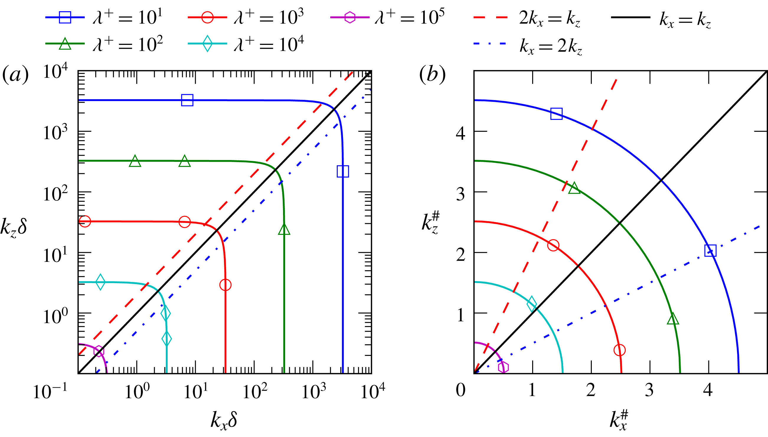
), however, there are several ways that a logarithmic scaling can be introduced. An obvious generalisation of the one-dimensional spectrum approach is to simply plot the log-spectral density in a two-dimensional ‘logarithmic Cartesian’ space, where the spectral log density is just
 $k_{x}k_{z}$
times the normal spectral density. This has been done by several previous authors (e.g. Jiménez & Hoyas Reference Jiménez and Hoyas2008; Mizuno & Jiménez Reference Mizuno and Jiménez2011; Chandran et al.
Reference Chandran, Baidya, Monty and Marusic2017; Kraheberger, Hoyas & Oberlack Reference Kraheberger, Hoyas and Oberlack2018). However, this has some shortcomings, two of which are as follows. (i) The orientation of the two-dimensional wavevector
 $(k_{x},k_{z})$
is distorted, making interpretation of the spectrum in terms of orientation and alignment of the Fourier modes difficult. Indeed, all lines of constant
 $k_{z}/k_{x}$
are mapped to lines with slope of 1, offset from the
 $k_{z}=k_{x}$
line by
 $\log k_{z}/k_{x}$
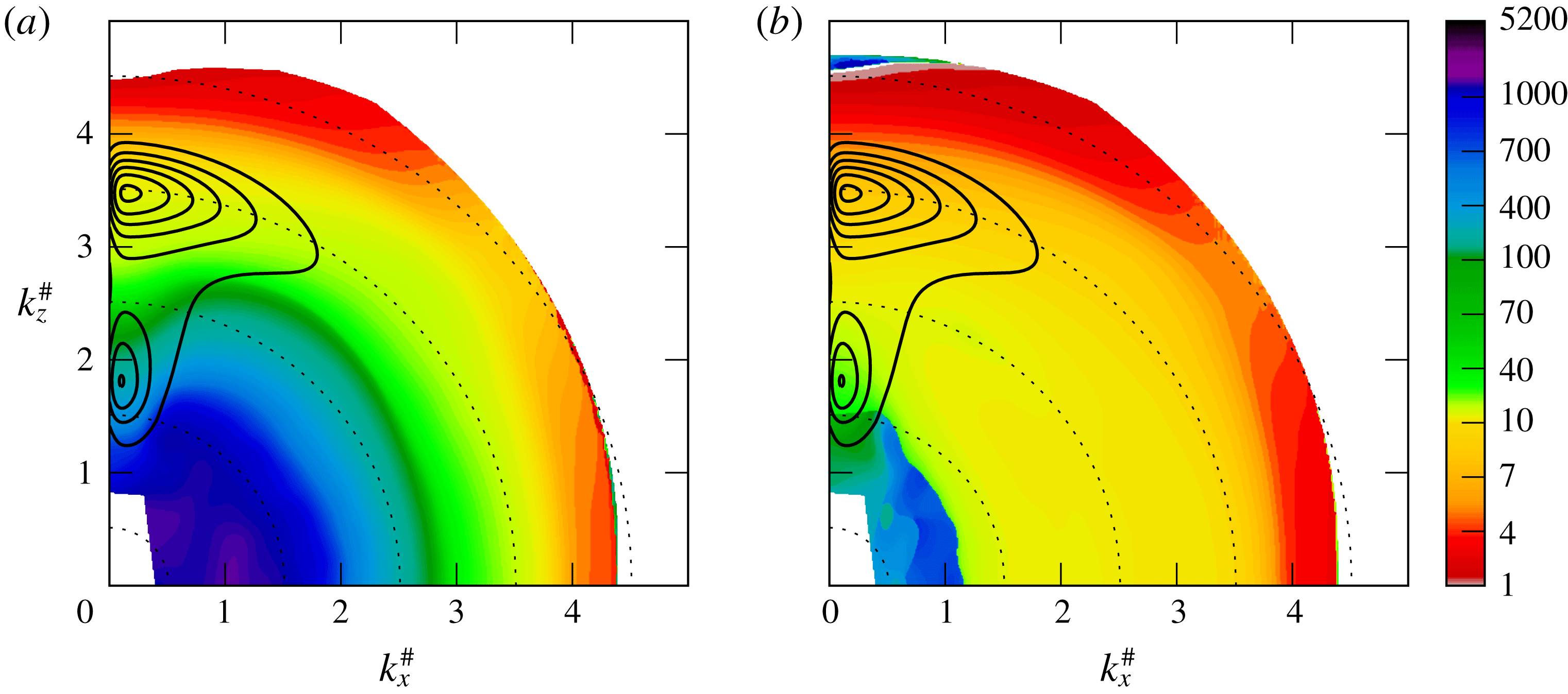
(see figure 1
a), obscuring how well aligned modes are with the
 $x$
and
 $z$
directions. (ii) Vector wavenumbers with the same magnitude
 $k=\sqrt{k_{x}^{2}+k_{z}^{2}}$
do not map onto a circle (see figure 1
a), making it difficult to assess scale isotropy in the spectrum.
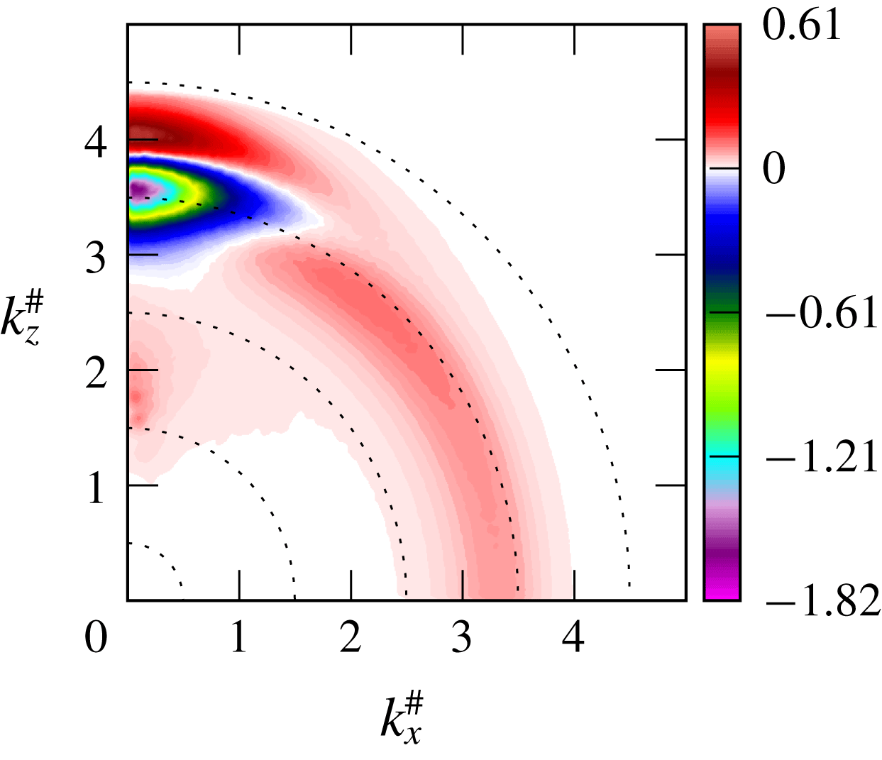
Comparison of (a) log-Cartesian and (b) log-polar coordinates for visualisation of two-dimensional spectra. In (a), the
 $\unicode[STIX]{x1D706}^{+}$
contours are shown for the R5200 case. In (b),
 $k_{x}^{\#}=(k_{x}/k)\log _{10}(k/k_{ref})$
and
 $k_{z}^{\#}=(k_{z}/k)\log _{10}(k/k_{ref})$
, where
 $k=(k_{x}^{2}+k_{z}^{2})^{1/2}$
and
 $k_{ref}\unicode[STIX]{x1D6FF}=Re_{\unicode[STIX]{x1D70F}}/50\,000$
(
 $k_{ref}^{+}=1/50\,000$
).

Both of these shortcomings can be overcome by representing the magnitude of the wavenumber
 $k$
on a logarithmic scale, rather than the individual wavenumber components, while preserving orientation in the logarithmic coordinate. To accomplish this, consider the spectral density
 $E$
expressed in ‘polar’ coordinates in wavenumber, that is,
 $k_{x}=k\cos \unicode[STIX]{x1D703}$
and
 $k_{z}=k\sin \unicode[STIX]{x1D703}$
. Then the integral of
 $E(k_{x},k_{z})=E(k\cos \unicode[STIX]{x1D703},k\sin \unicode[STIX]{x1D703})$
in
 $k_{x}$
and
 $k_{z}$
can be rewritten
 $$\begin{eqnarray}\int _{k_{x}>0}\int _{k_{z}>0}E\,\text{d}k_{x}\,\text{d}k_{z}=\int _{\unicode[STIX]{x1D703}=0}^{\unicode[STIX]{x03C0}/2}\int _{k>0}E\,k\,\text{d}k\,\text{d}\unicode[STIX]{x1D703}.\end{eqnarray}$$
Now, we want to plot in a space that is logarithmic in
 $k$
, so define
 $\unicode[STIX]{x1D709}=\log (k/k_{ref})$
, where
 $k_{ref}$
is an arbitrary reference wavenumber, which must be smaller than the smallest non-zero wavenumber included in the spectrum. The ‘logarithmic polar’ coordinates would be
 $\unicode[STIX]{x1D709}$
and
 $\unicode[STIX]{x1D703}$
, while the associated Cartesian coordinates would be
 $k_{x}^{\#}=\unicode[STIX]{x1D709}\cos \unicode[STIX]{x1D703}=\unicode[STIX]{x1D709}k_{x}/k$
and
 $k_{z}^{\#}=\unicode[STIX]{x1D709}\sin \unicode[STIX]{x1D703}=\unicode[STIX]{x1D709}k_{z}/k$
. Re-expressing the integral (2.26) in terms of
 $\unicode[STIX]{x1D709}$
yields
 $$\begin{eqnarray}\int _{k_{x}>0}\int _{k_{z}>0}E\,\text{d}k_{x}\,\text{d}k_{z}=\int _{\unicode[STIX]{x1D703}=0}^{\unicode[STIX]{x03C0}/2}\int _{\unicode[STIX]{x1D709}>0}\frac{k^{2}}{\unicode[STIX]{x1D709}}E\,\unicode[STIX]{x1D709}\,\text{d}\unicode[STIX]{x1D709}\,\text{d}\unicode[STIX]{x1D703}=\int _{k_{x}^{\#}>0}\int _{k_{z}^{\#}>0}\frac{k^{2}}{\unicode[STIX]{x1D709}}E\,\text{d}k_{x}^{\#}\,\text{d}k_{z}^{\#}.\end{eqnarray}$$
So, the desired two-dimensional spectral density in a space that is logarithmic in
 $k$
is plotted as a function of
 $k_{x}^{\#}$
and
 $k_{z}^{\#}$
, and to preserve the integral in this transformed space, the log-polar spectral density should be
 $k^{2}/\unicode[STIX]{x1D709}$
times the normal spectral density. As shown in figure 1(b), in this space, lines of constant
 $k_{z}/k_{x}$
have slopes of
 $k_{z}/k_{x}$
, and contours of constant
 $k$
are circles. The contours of constant
 $k$
are labelled according to their wavelength
 $\unicode[STIX]{x1D706}=2\unicode[STIX]{x03C0}/k$
, which will be done throughout to facilitate connection with well-known length scales.
In the remainder of the paper, all quantities that are essentially densities, such as Reynolds stress components, terms in the RSTE and their spectra, will be plotted in logarithmic coordinates in
 $y$
and/or wavenumber. They will be plotted as densities in the logarithmic coordinates used, so that the visualisation depicts the distribution of the relevant quantity in those coordinates. Further, in the case of two-dimensional spectra, log-polar coordinates as defined above will be used, with
 $k_{ref}\unicode[STIX]{x1D6FF}=Re_{\unicode[STIX]{x1D70F}}/50\,000$
(
 $k_{ref}^{+}=1/50\,000$
), as shown in figure 1(b), and log-polar spectral densities will be depicted. Using a
 $k_{ref}^{+}$
that is independent of Reynolds number will allow spectral features that scale in wall units to be directly compared for different wavenumbers. The DNS calculations naturally yield two-dimensional spectra represented on a Cartesian grid in
 $k_{x}$
and
 $k_{z}$
. To produce the log-polar spectra, these are interpolated onto a Cartesian grid in
 $k_{x}^{\#}$
and
 $k_{z}^{\#}$
with grid spacings of 0.01, and the results are smoothed using a Gaussian kernel with
 $\unicode[STIX]{x1D70E}=0.06$
. In what follows, the terms ‘spectrum’ and ‘spectra’ will be used to mean the spectral density associated with the logarithmic space in which it is plotted. Finally, unless otherwise indicated, all plotted and visualised quantities are normalised in wall units.
3 Results
In this section, the results of a detailed spectral analysis of the transport equations for the velocity variances in channel flow are presented. We begin with the velocity variance spectra themselves, followed by analysis of the terms in the transport equations, as described in § 2. Finally, we discuss the Reynolds number independence of the small-scale contributions to the transport equations.
As described in § 2.3, the quantities visualised in this paper are densities, in the logarithmic space in which they are plotted. For the velocity variances, these are energy densities, representing the distribution of energy in
 $y$
and the wavenumber space. However, for the terms on the right-hand side of the transport equations (2.24), these are densities of the sources (when positive) and sinks (when negative) of the velocity variances. Of course, the only true source of turbulent energy is production, and the only true sink is dissipation. The other terms transport energy in
 $y$
and transfer it between scales and between components. For these terms, we will commonly refer to regions of positive density as ‘recipient’ regions and regions of negative density as ‘donor’ regions, to reflect the fact that energy is being redistributed from donor (negative) regions to recipient (positive) regions. In the following, detailed interpretation of where energy is being transferred from and to will depend on the characteristics of the individual terms, and indeed they have been formulated to allow such interpretation to the extent possible.
3.1 Energy spectra
Two-dimensional spectra of
 $\langle u^{\prime 2}\rangle$
,
 $\langle v^{\prime 2}\rangle$
and
 $\langle w^{\prime 2}\rangle$
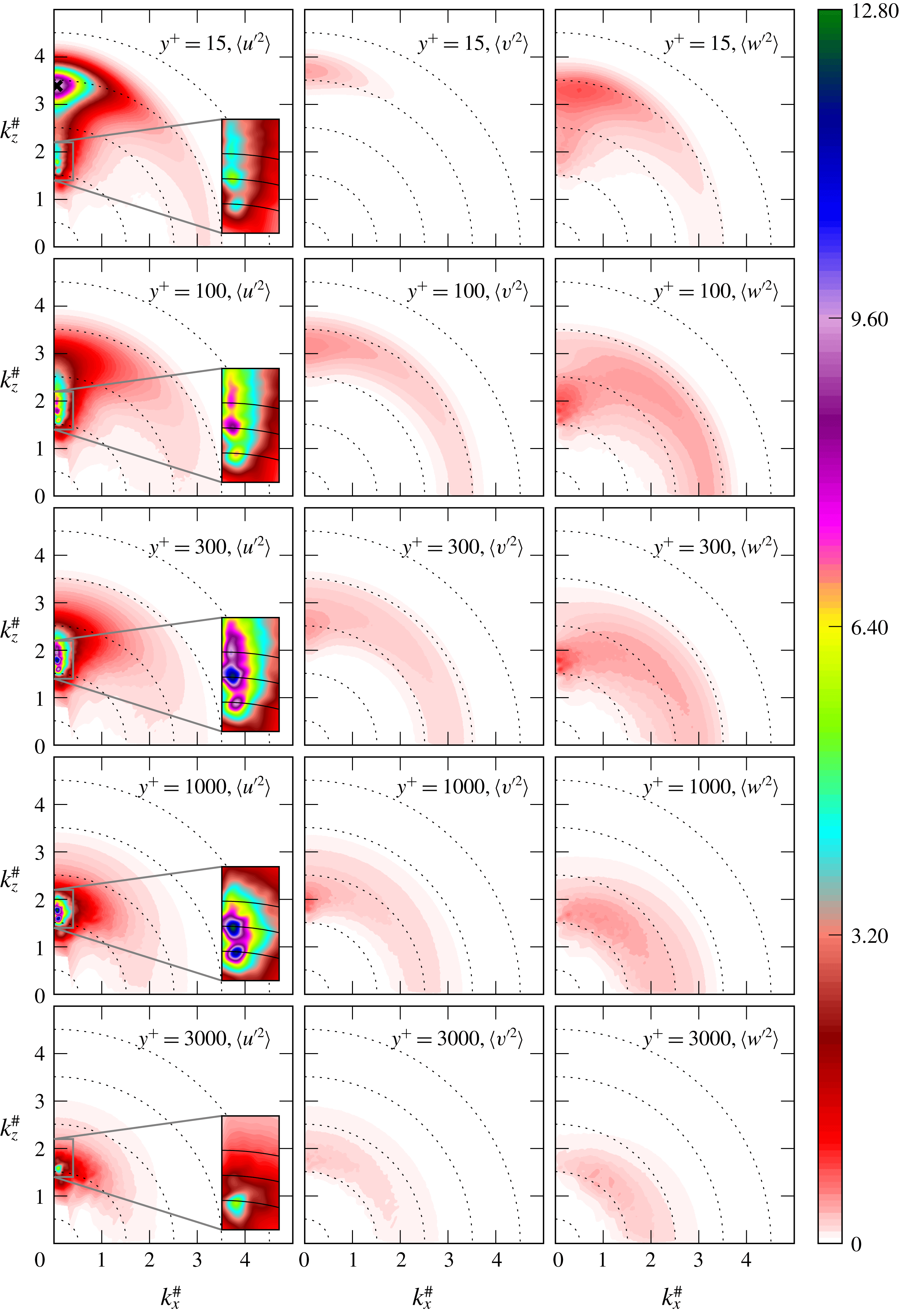
in log-polar coordinates, as defined in figure 1, from R5200;
 $\unicode[STIX]{x1D706}^{+}=10$
on the outermost dotted circle and increases by a factor of 10 for each dotted circle moving inward. In the magnified insets,
 $\unicode[STIX]{x1D706}/\unicode[STIX]{x1D6FF}=0.67$
on the top-most solid line and increases by a factor of 1.5 for each solid line moving downward. The symbol
 $\times$
marks a feature described in the text.

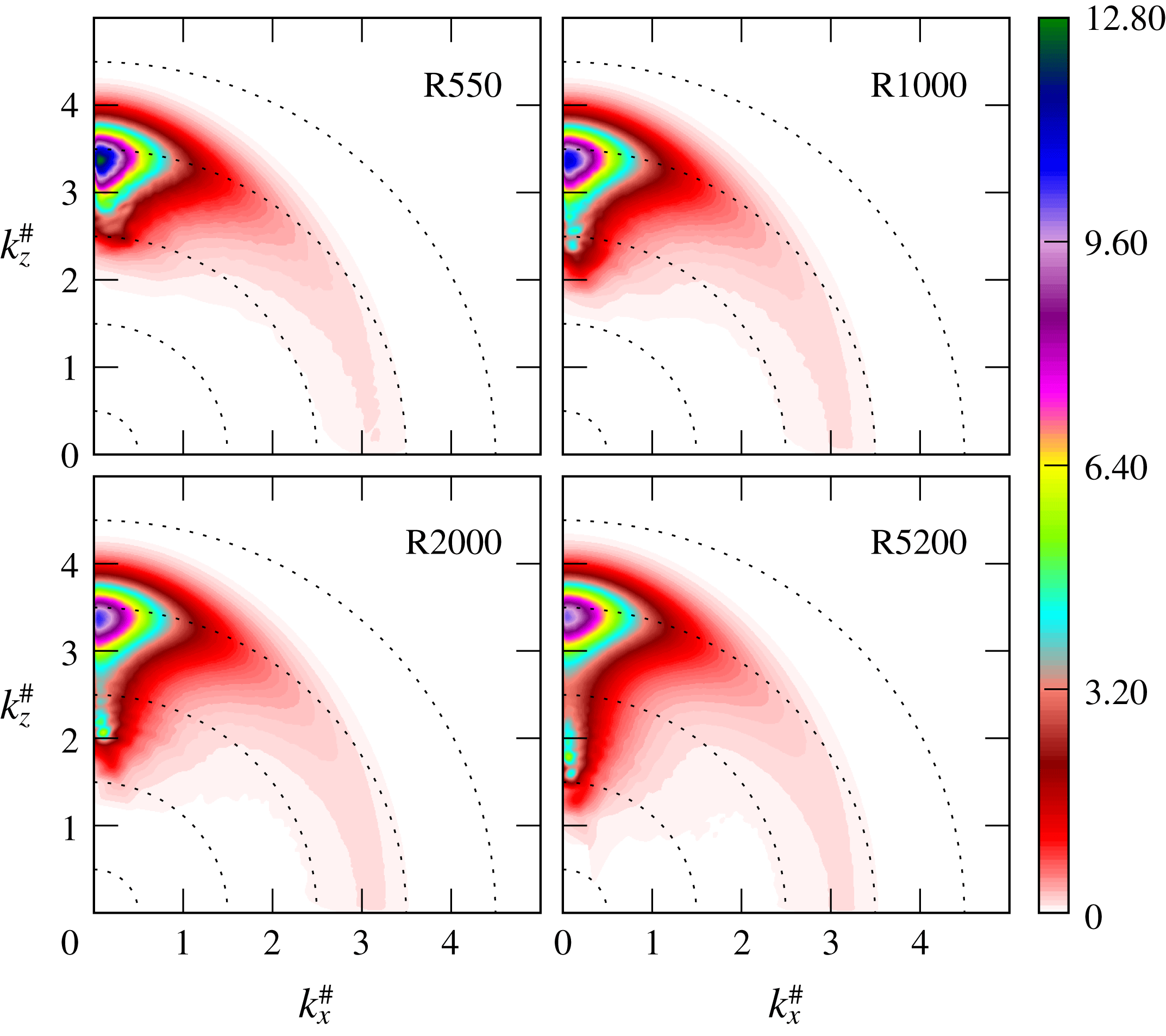
Two-dimensional spectra of
 $\langle u^{\prime 2}\rangle$
in log-polar coordinates, as defined in figure 1, at
 $y^{+}=15$
;
 $\unicode[STIX]{x1D706}^{+}=10$
on the outermost dotted circle and increases by a factor of 10 for each dotted circle moving inward.

The primary objective of the current study is to characterise the flow of turbulent energy underlying the distribution of energy in high Reynolds number wall-bounded turbulence. It is useful to begin this exploration by examining this energy distribution. To this end, the two-dimensional
 $\langle u^{\prime 2}\rangle$
,
 $\langle v^{\prime 2}\rangle$
and
 $\langle w^{\prime 2}\rangle$
energy spectra are plotted at several
 $y$
-locations in the log-polar space described above (figure 2). The most obvious feature of these spectra is the extreme concentration of energy in the spectrum of
 $\langle u^{\prime 2}\rangle$
into regions along the
 $k_{z}^{\#}$
axis, that is, Fourier modes with
 $k_{z}/k_{x}\gtrsim 10$
. These are associated with structures that are strongly elongated in the
 $x$
direction (inclination angle less than
 $6^{\circ }$
). Near the wall (
 $y^{+}=15$
), this is expected as a consequence of the well-known low- and high-speed near-wall streaks. At
 $y^{+}=15$
, the high energy region is distributed around
 $\unicode[STIX]{x1D706}^{+}\approx 100$
, consistent with expectations for the spacing of the streaks. Note, however, that the energy density peaks along the axis at
 $\unicode[STIX]{x1D706}^{+}\approx 140$
and the energy distribution extends to significantly larger spanwise scales. The triangular region of high energy density that extends to approximately
 $\unicode[STIX]{x1D706}^{+}=1000$
(marked with a
 $\times$
in figure 2) is a consequence of the autonomous near-wall dynamics described by Hamilton et al. (Reference Hamilton, Kim and Waleffe1995) and Jiménez & Pinelli (Reference Jiménez and Pinelli1999), and is similar in the two-dimensional
 $\langle u^{\prime 2}\rangle$
spectra at lower Reynolds numbers (see figure 3). Note, however, that the magnitude of the
 $\langle u^{\prime 2}\rangle$
spectral peak is slowly decreasing with increasing Reynolds number, so that the peak at
 $Re_{\unicode[STIX]{x1D70F}}=5200$
is approximately 30 % lower than at
 $Re_{\unicode[STIX]{x1D70F}}=550$
. This will be discussed in more detail below.
Farther from the wall (
 $y^{+}>100$
), there are again strong peaks, but at much longer wavelengths (
 $1000<\unicode[STIX]{x1D706}^{+}<10\,000$
). Notice that at
 $y^{+}=300$
, there are actually three distinct peaks in the spectrum, all located along the
 $k_{z}^{\#}$
axis, with (spanwise) wavelengths
 $\unicode[STIX]{x1D706}^{+}\approx 3400$
, 5200 and 7800, or
 $\unicode[STIX]{x1D706}/\unicode[STIX]{x1D6FF}\approx 0.67$
, 1.0 and 1.5, which are separated by approximately a factor of 1.5. At
 $y^{+}=100$
, all three peaks are present, although the long wavelength one (lower on the figure) is much weaker. Farther from the wall, at
 $y^{+}=1000$
, the short wavelength peak is absent, and the other two are approximately the same strength, and at
 $y^{+}=3000$
, only the longest wavelength peak is present. This suggests that there is a discrete hierarchy of spanwise streak scales, with each dominant in a different range of
 $y$
(longer
 $\unicode[STIX]{x1D706}$
at larger
 $y$
). Note that similar discrete peaks in spanwise scales are also observed in DNSs of pipe flows at
 $Re_{\unicode[STIX]{x1D70F}}=3000$
(see figure 10 in Ahn et al.
Reference Ahn, Lee, Lee, Kang and Sung2015). Previously published one-dimensional spanwise
 $\langle u^{\prime 2}\rangle$
spectra have indicated the presence of discrete spectral peaks in channels, such as figures 2(b) in del Álamo & Jiménez (Reference del Álamo and Jiménez2003) and 8(b) in Lee & Moser (Reference Lee and Moser2015a
), although low Reynolds number (
 $Re_{\unicode[STIX]{x1D70F}}=550$
) effects are likely in del Álamo & Jiménez (Reference del Álamo and Jiménez2003).
The mechanism by which such a discrete scale hierarchy might arise is not clear. It is probably not a direct consequence of the finite computational domain size, since the spanwise domain size is approximately six times the largest dominant wavelength. In addition, the R550 case exhibits discrete peaks in the spanwise one-dimensional spectra (not shown) at approximately the same values of
 $k_{z}\unicode[STIX]{x1D6FF}$
as in del Álamo & Jiménez (Reference del Álamo and Jiménez2003), despite the fact that the spanwise domain sizes are significantly different (
 $3\unicode[STIX]{x03C0}\unicode[STIX]{x1D6FF}$
here and
 $4\unicode[STIX]{x03C0}\unicode[STIX]{x1D6FF}$
in del Álamo & Jiménez Reference del Álamo and Jiménez2003). This provides support for the hypothesis that these discrete spectra are not driven by domain size effects. However, the low Reynolds number in these cases makes this far from definitive. On the other hand, the fact that the domain size is only six times the longest wavelength means that the variation of the spectra near the long wavelength peak is not well resolved. For example, there are just three points in the discrete spectrum between the two longest wavelength peaks. It is thus possible that misleading artefacts are present, although it seems that the wave-space resolution should be sufficient to at least distinguish these peaks. One possible physical explanation is that a combination or phase locking of smaller structures could be creating larger aggregates, as suggested by Tomkins & Adrian (Reference Tomkins and Adrian2003).
In addition to the dominance of these spanwise scales far from the wall, the outer scales appear to be imprinted on the spectra nearer to the wall, including at
 $y^{+}=15$
, where three weak peaks are present at the same wavenumbers. This suggests that these features of the near-wall spectral structure are imposed from the outer flow, consistent with suggestions by Hutchins & Marusic (Reference Hutchins and Marusic2007b
) and Marusic et al. (Reference Marusic, Mathis and Hutchins2010b
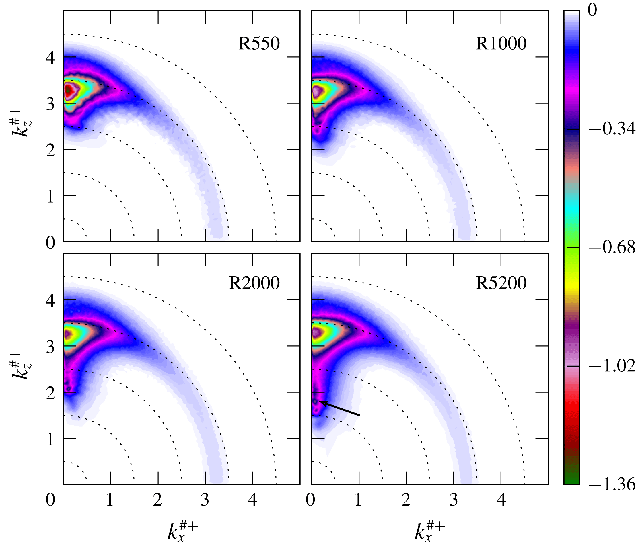
), and would therefore be different at different Reynolds numbers. As is apparent in figure 3, this is indeed the case. At the lower Reynolds numbers, there are fewer of these weak large wavelength peaks. Since the shorter wavelength features of the spectra are similar at different Reynolds numbers due to the autonomous near-wall dynamics, these outer flow imprints on the near-wall region appear to be responsible for the Reynolds number dependence of the near-wall peak of
 $\langle u^{\prime 2}\rangle$
as suggested by Hutchins & Marusic (Reference Hutchins and Marusic2007a
) and Marusic et al. (Reference Marusic, Mathis and Hutchins2010a
). Indeed, applying a high-pass filter that eliminates wavenumbers with
 $\unicode[STIX]{x1D706}^{+}>1000$
also eliminates the near-wall Reynolds number dependence of
 $\langle u^{\prime 2}\rangle$
(see § 3.7).
The large-scale features of the near-wall turbulence that are imposed from the outer flow will also interact nonlinearly with the autonomous near-wall turbulence. Particularly, the large-scale fluctuations in the streamwise velocity implied by the spectrum will result in large-scale variations in the near-wall shear. The autonomous near-wall dynamics will therefore by modulated by these variations, as suggested by Hutchins & Marusic (Reference Hutchins and Marusic2007b ) and Marusic et al. (Reference Marusic, Mathis and Hutchins2010b ), resulting particularly in local variations in the dominant wavelength. This results in a reduction of magnitude of the small-scale spectral peak with increasing Reynolds number, as described above, due to increasing large-scale fluctuations with Reynolds number. However, because the near-wall scaling for energy is linear in shear, these large-scale modulations in shear do not result in a net change in the turbulent energy associated with the near-wall autonomous dynamics. Thus, increasing Reynolds number will not affect the small-scale energy, consistent with the high-pass filtering observations described above. The reduction with Reynolds number of the magnitude of the small-scale spectral peak is difficult to see in figure 3, but was confirmed in plots of the difference in spectra at different Reynolds numbers (not shown).
Near the wall, the
 $\langle v^{\prime 2}\rangle$
and
 $\langle w^{\prime 2}\rangle$
spectra are also strongest in the wavenumber regimes in which
 $\langle u^{\prime 2}\rangle$
is so strongly peaked, that is, modes with large
 $k_{z}/k_{x}$
(elongated in the
 $x$
direction). However, the spectra are not nearly as strongly peaked as in the
 $\langle u^{\prime 2}\rangle$
spectrum. Farther from the wall, there is a similar structure with weak concentrations of energy in modes for which
 $\langle u^{\prime 2}\rangle$
is strongly peaked, although this appears to get weaker with increasing
 $y$
until, at
 $y^{+}=3000$
(
 $y/\unicode[STIX]{x1D6FF}\approx 0.6$
), it is not discernible. In all the velocity components, some energy is also distributed more-or-less isotropically over a range of
 $\unicode[STIX]{x1D706}$
of a decade or more (an approximately circular band in figure 2). However, the range in
 $\unicode[STIX]{x1D706}^{+}$
of this band depends on
 $y$
, and for
 $y^{+}\geqslant 100$
, the
 $\unicode[STIX]{x1D706}^{+}$
in the centre of the band is approximately proportional to
 $y$
, as would be expected in the scale similarity range connected with the log law. The spectra thus appear to be a combination of classical turbulence that is nearly isotropic in scale and component, and the strongly streaky streamwise velocity discussed above along with corresponding streaky fluctuations in
 $\langle v^{\prime 2}\rangle$
and
 $\langle w^{\prime 2}\rangle$
.
3.2 Production
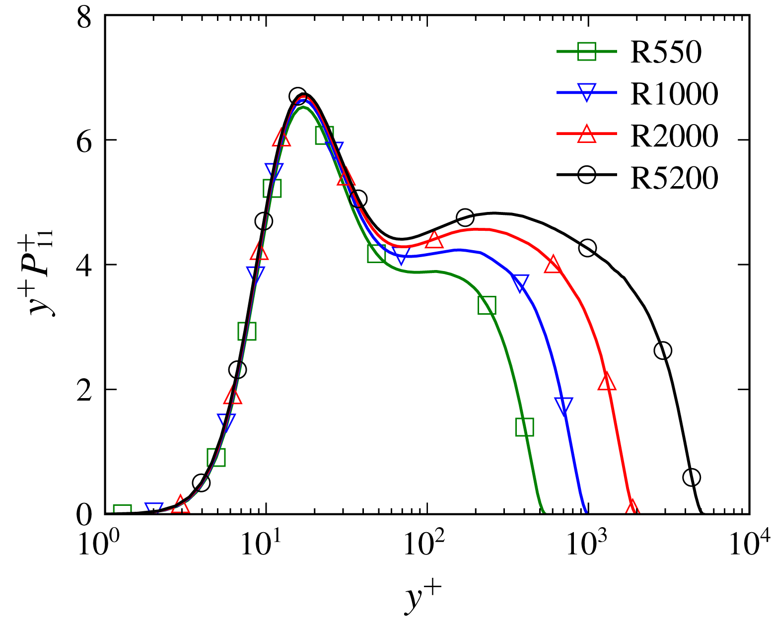
Profiles of
 $\langle u^{\prime 2}\rangle$
production as log densities.

One-dimensional streamwise and spanwise spectral densities of
 $\unicode[STIX]{x1D617}_{11}$
. Solid lines are at
 $k_{x}y=0.5$
and
 $k_{z}y=2$
. The symbol
 $\times$
marks features described in the text.

The one-dimensional profile of production of
 $\langle u^{\prime 2}\rangle$
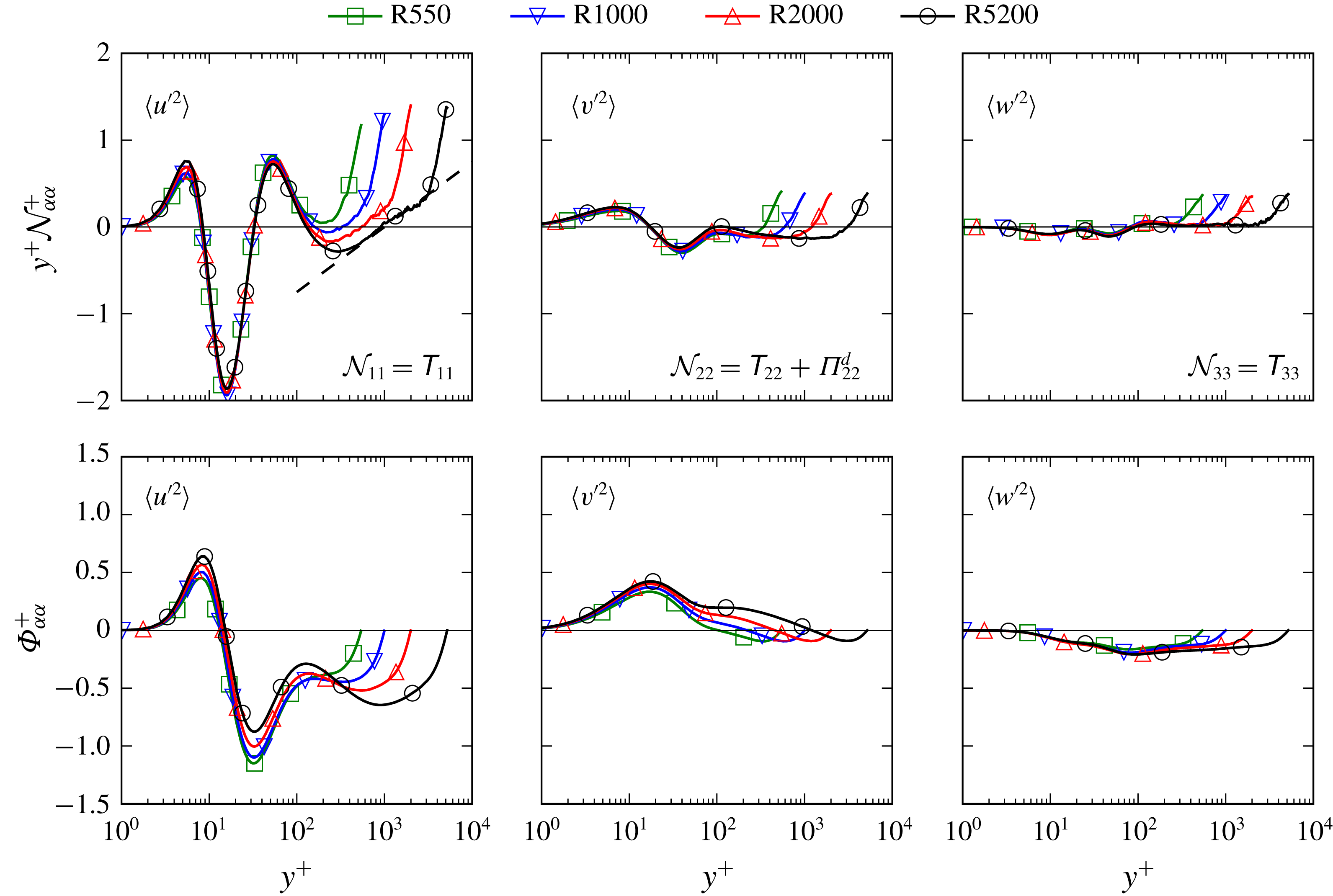
is shown in figure 4, which, because the production of
 $\langle v^{\prime 2}\rangle$
and
 $\langle w^{\prime 2}\rangle$
is zero, is also twice the production of turbulent kinetic energy. There are only weak
 $Re$
dependences in the production up to
 $y^{+}\approx 70$
. On the other hand, the contribution to the production from regions away from the wall (say
 $y^{+}>70$
) increases continuously with the
 $Re$
, with approximately 50 % of
 $\langle u^{\prime 2}\rangle$
production occurring in the region
 $y^{+}>70$
at
 $Re_{\unicode[STIX]{x1D70F}}=2000$
. This is not just because the domain is getting larger in plus units, but also because in the outer region the production is increasing with Reynolds number at constant
 $y^{+}$
. From the definition of
 $\unicode[STIX]{x1D617}_{11}^{+}$
, in the log region,
 $$\begin{eqnarray}y^{+}\unicode[STIX]{x1D617}_{11}^{+}=-2y^{+}\langle u^{\prime }v^{\prime }\rangle ^{+}\frac{\unicode[STIX]{x2202}U^{+}}{\unicode[STIX]{x2202}y^{+}}\approx -\frac{2}{\unicode[STIX]{x1D705}}\langle u^{\prime }v^{\prime }\rangle ^{+},\end{eqnarray}$$
where
 $\unicode[STIX]{x1D705}$
is the von Kármán constant, which is approximately 0.384 in the R5200 case (Lee & Moser Reference Lee and Moser2015a
). Presuming
 $\unicode[STIX]{x1D705}$
does not change as
 $Re$
increases,
 $y^{+}\unicode[STIX]{x1D617}_{11}^{+}$
depends only on
 $\langle u^{\prime }v^{\prime }\rangle ^{+}$
in the log region. The theoretical minimum of
 $\langle u^{\prime }v^{\prime }\rangle ^{+}$
at infinite
 $Re$
is
 $-1$
, so the maximum of
 $y^{+}\unicode[STIX]{x1D617}_{11}^{+}$
for
 $y^{+}>70$
approaches
 $2/\unicode[STIX]{x1D705}\approx 5.21$
as
 $Re$
increases. The maximum value of
 $y^{+}\unicode[STIX]{x1D617}_{11}^{+}$
in R5200 is 4.83, which is 92.7 % of the theoretical maximum. Also, asymptotically for large
 $Re$
,
 $-\langle u^{\prime }v^{\prime }\rangle _{max}\approx 1-2/\sqrt{\unicode[STIX]{x1D705}Re_{\unicode[STIX]{x1D70F}}}$
(Lee & Moser Reference Lee and Moser2015a
; Afzal Reference Afzal1982). Hence, a flow at
 $Re_{\unicode[STIX]{x1D70F}}\approx 10^{5}$
is required for the outer peak of
 $y^{+}\unicode[STIX]{x1D617}_{11}^{+}$
to be within 1 % of theoretical maximum, as for
 $\langle u^{\prime }v^{\prime }\rangle ^{+}$
. This means that the contribution of the outer flow to the production keeps increasing as
 $Re$
increases and the production in the overlap region scales as
 $y^{-1}$
for large Reynolds number, i.e.
 $\unicode[STIX]{x1D617}_{11}^{+}=5.21/y^{+}$
, as noted by Hoyas & Jiménez (Reference Hoyas and Jiménez2008).
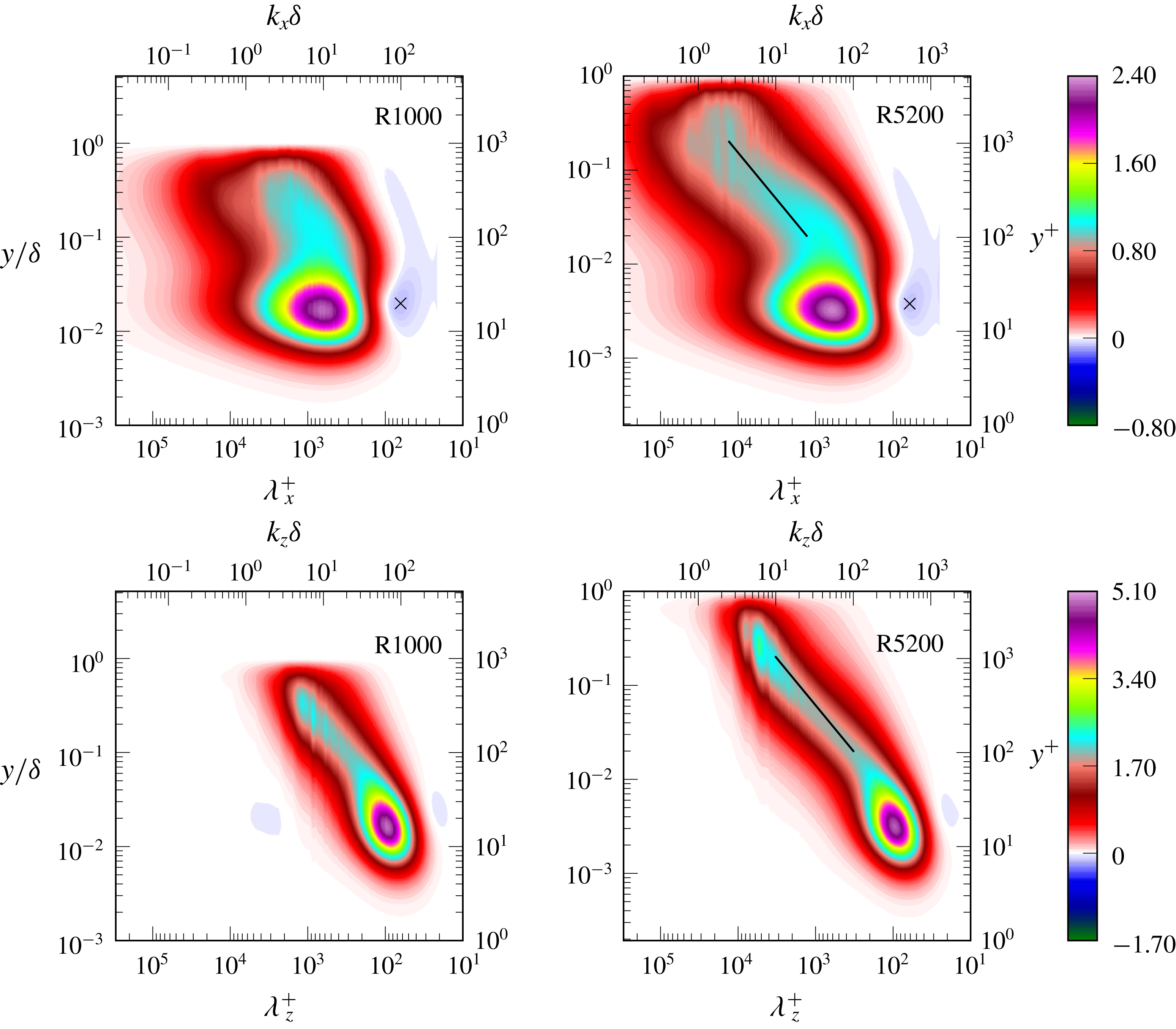
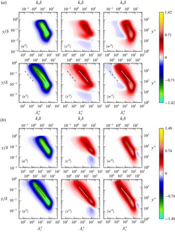
The
 $y$
- and
 $k$
-premultiplied one-dimensional spectral density of
 $\langle u^{\prime 2}\rangle$
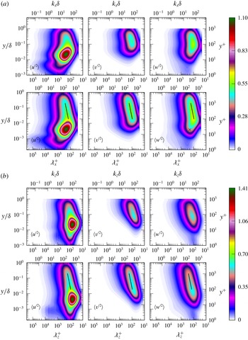
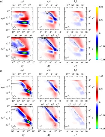
production is shown in figure 5. The appearance of the
 $\langle u^{\prime 2}\rangle$
production spectra are inherently similar to those of
 $\langle u^{\prime }v^{\prime }\rangle$
presented in Lee & Moser (Reference Lee and Moser2015a
) because in the log region,
 $$\begin{eqnarray}y^{+}\unicode[STIX]{x1D60C}_{11}^{P+}=-2y^{+}\unicode[STIX]{x1D60C}_{12}^{+}\frac{\unicode[STIX]{x2202}U^{+}}{\unicode[STIX]{x2202}y^{+}}=-\frac{2}{\unicode[STIX]{x1D705}}\unicode[STIX]{x1D60C}_{12}^{+}.\end{eqnarray}$$
The production spectra of R1000 and R5200 are similar in several respects up to
 $y^{+}\approx 70$
. First, the inner peaks are located at
 $\unicode[STIX]{x1D706}_{x}^{+}\approx 600$
,
 $\unicode[STIX]{x1D706}_{z}^{+}\approx 100$
and
 $y^{+}\approx 15$
. Second, similar to
 $\langle u^{\prime }v^{\prime }\rangle$
, there is weak negative production of
 $\langle u^{\prime 2}\rangle$
around
 $\unicode[STIX]{x1D706}_{x}^{+}\approx 60$
and
 $y^{+}\approx 20$
in the streamwise spectral density (marked with
 $\times$
). Finally, the streamwise spectral density contours are similar in R1000 and R5200 up to
 $y^{+}\approx 70$
, while
 $Re$
dependences are stronger for
 $y^{+}>70$
. An outer peak in the spanwise spectrum occurs at
 $k_{z}\unicode[STIX]{x1D6FF}\approx 6$
and
 $y/\unicode[STIX]{x1D6FF}\approx 0.3$
in both cases, but R5200 has a much stronger outer peak. The outer peak in the streamwise spectrum of R5200 is diffuse, making a definitive determination of its location difficult (figure 5). The distinction of inner and outer peaks in the
 $\langle u^{\prime 2}\rangle$
production spectra is consistent with the work of Cimarelli et al. (Reference Cimarelli, De Angelis and Casciola2013), and as they noted, the existence of outer scale production suggests a self-sustaining mechanism of the large-scale motion. In the overlap region, the wavenumbers at which the production spectra are maximum scale as
 $y^{-1}$
from
 $y^{+}\approx 100$
to
 $y/\unicode[STIX]{x1D6FF}\approx 0.2$
in R5200. This is because the premultiplied spectral density of
 $\langle u^{\prime }v^{\prime }\rangle$
in the overlap region scales as
 $y^{-1}$
, consistent with the observation of Jiménez & Hoyas (Reference Jiménez and Hoyas2008). As noted above, the
 $\langle u^{\prime 2}\rangle$
production approaches a
 $y^{-1}$
scaling in the overlap region, which would imply a plateau in figure 4 at high
 $Re$
.
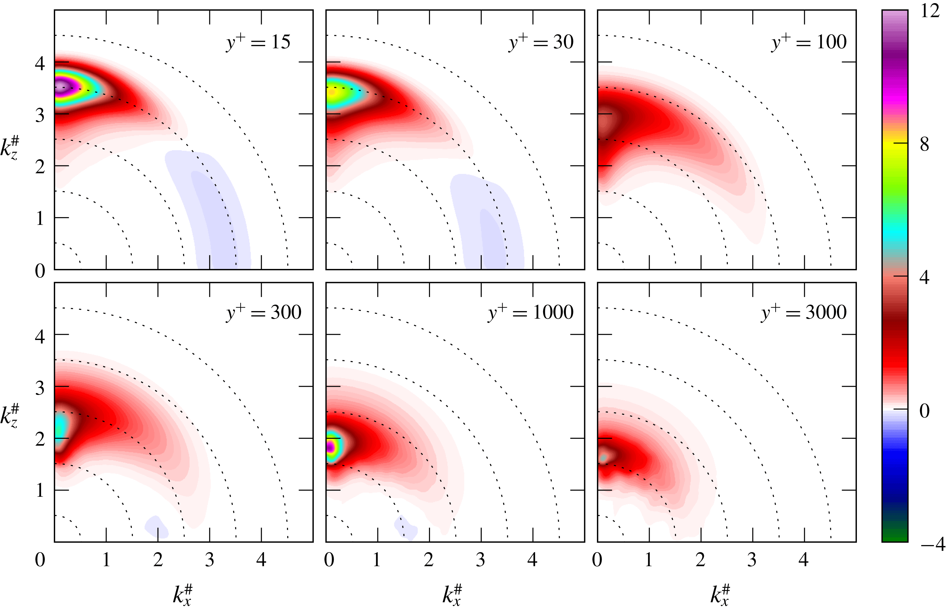
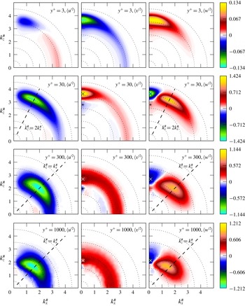
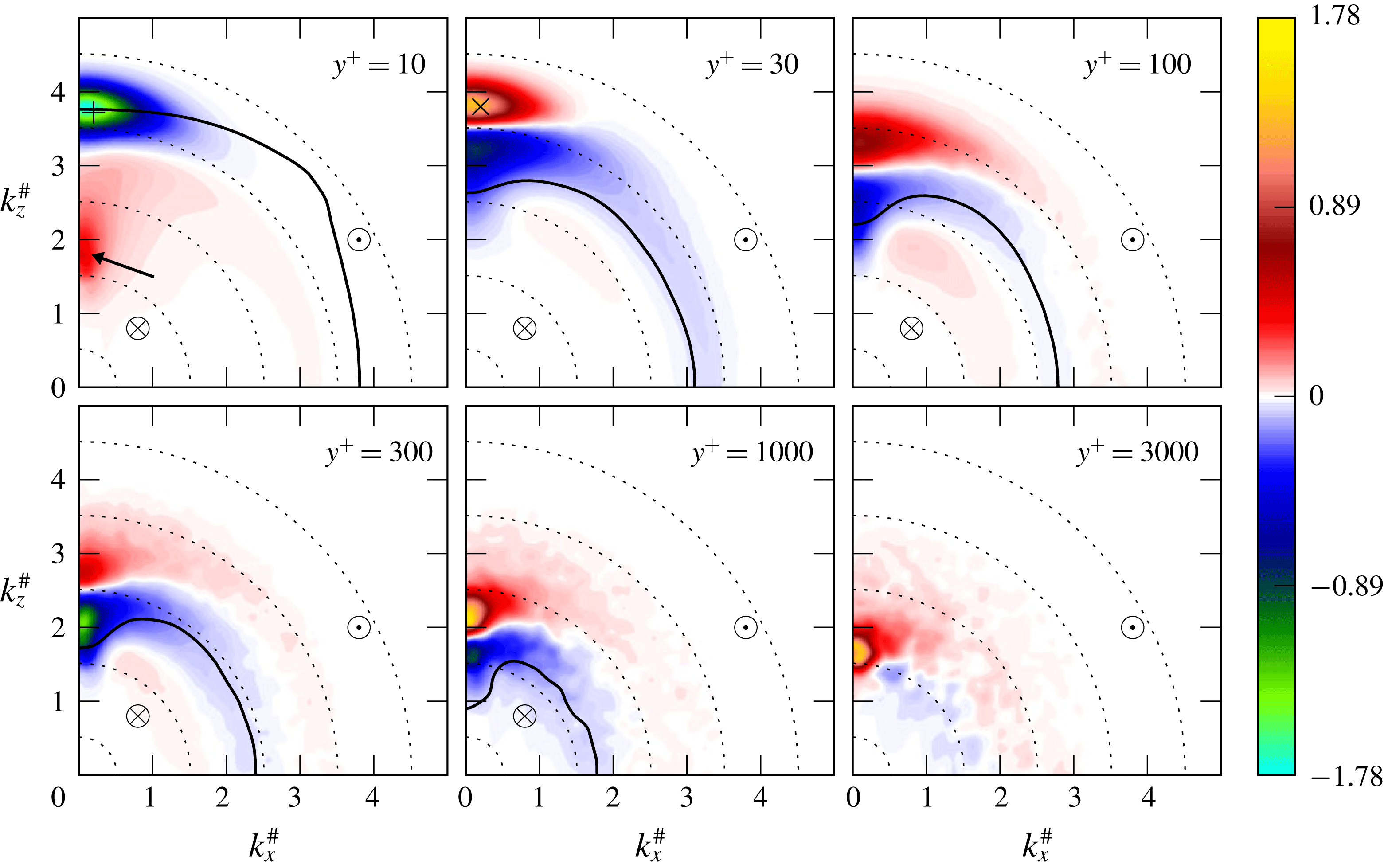
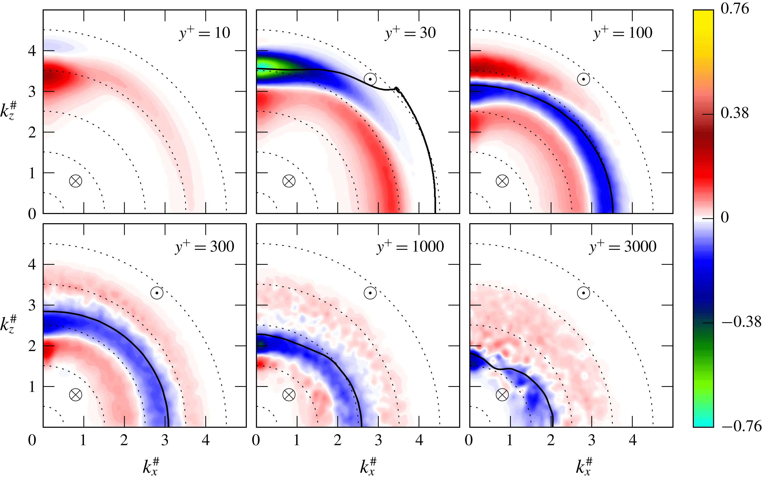
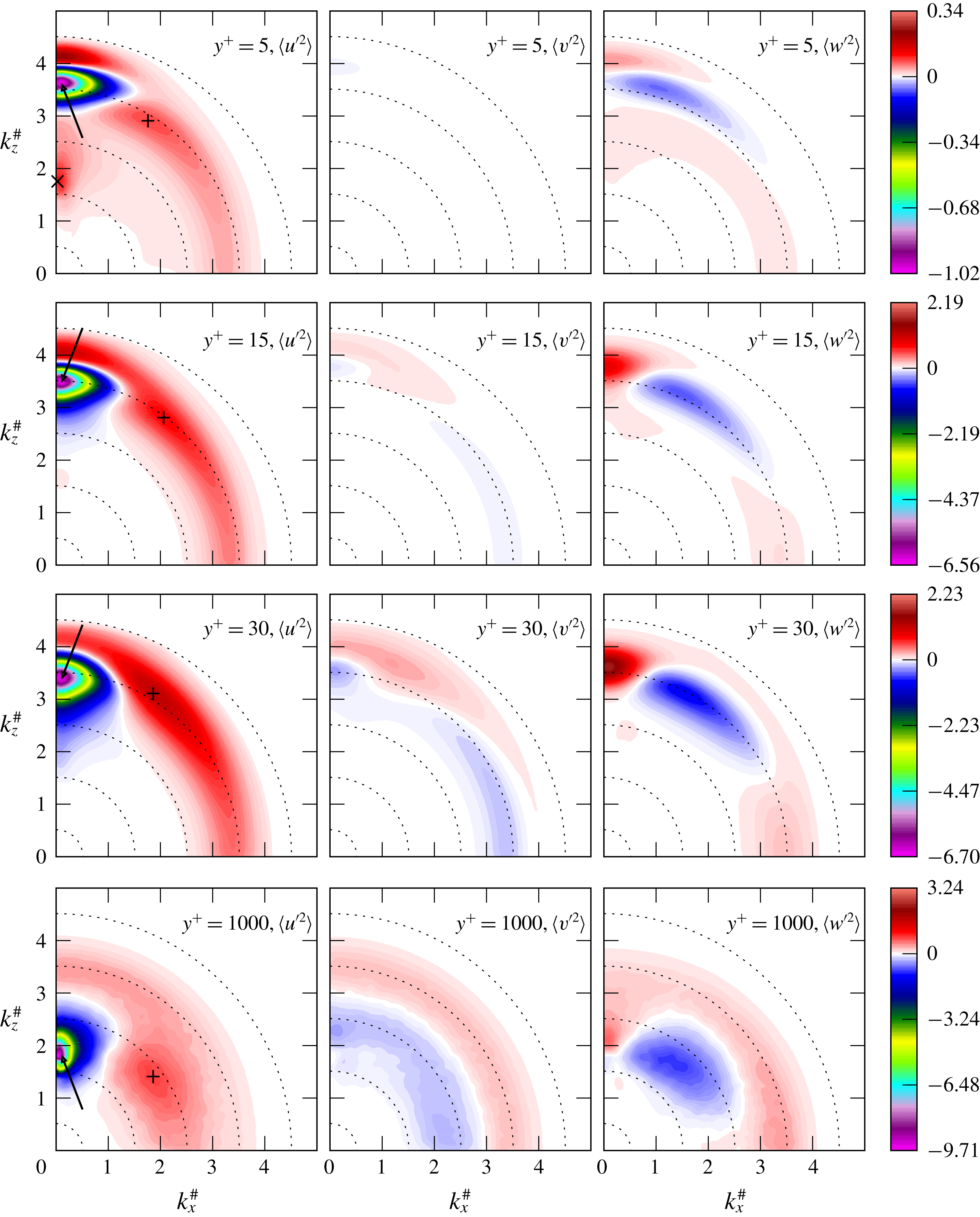
More insight into the spectral structure of the production can be gained from the two-dimensional spectra shown in figure 6. Unsurprisingly, the production is concentrated along the
 $k_{z}^{\#}$
axis, as in the
 $\langle u^{\prime 2}\rangle$
spectra (figure 2), with spectral peaks that correspond to the peaks in
 $\langle u^{\prime 2}\rangle$
spectra. However, there are several significant differences. Very near the wall (
 $y^{+}=15$
or 30), there are no discrete long wave spectral peaks along the
 $k_{z}^{\#}$
axis as there are in the
 $\langle u^{\prime 2}\rangle$
spectra. This is expected since these
 $\langle u^{\prime 2}\rangle$
spectral peaks appeared to be imposed from the outer region turbulence (see discussion in § 3.1), and so the energy in them would be transported in
 $y$
or transferred in scale, rather than produced locally. In addition, farther from the wall, there is only one dominant production spectral peak at each
 $y$
-location shown, indicating that the more complex multi-peak characteristics of the
 $\langle u^{\prime 2}\rangle$
spectra at these locations are also likely due to wall-normal transport. An examination of the two-dimensional production spectra as a continuous function of
 $y$
shows that the production peak at
 $\unicode[STIX]{x1D706}/\unicode[STIX]{x1D6FF}\approx 1.5$
is dominant for
 $y/\unicode[STIX]{x1D6FF}>0.35$
, and the one at
 $\unicode[STIX]{x1D706}/\unicode[STIX]{x1D6FF}\approx 1.0$
is dominant from
 $0.1<y/\unicode[STIX]{x1D6FF}<0.35$
. The lower bound of the region where there is a
 $\unicode[STIX]{x1D706}/\unicode[STIX]{x1D6FF}\approx 0.67$
peak is not distinct. In a region around the change in dominant production scale, two distinct peaks are present. These discrete production peaks are consistent with the discrete set of spectral peaks in the
 $\langle u^{\prime 2}\rangle$
spectra.
Two-dimensional spectral density of
 $\unicode[STIX]{x1D617}_{11}$
in log-polar coordinates, as defined in figure 1, from R5200;
 $\unicode[STIX]{x1D706}^{+}=10$
on the outermost dotted circle and increases by a factor of 10 for each dotted circle moving inward.

Other interesting features of the two-dimensional production spectra are the regions of negative production, especially near the wall. This is clearly the negative production that gives rise to the negative regions in the one-dimensional
 $k_{x}$
production spectra. Near the wall (
 $y^{+}=15$
), negative production occurs over a range of scales around
 $\unicode[STIX]{x1D706}^{+}=100$
, for modes with wavevectors oriented more in the streamwise direction than the spanwise direction. Farther from the wall, negative production occurs with wavevectors oriented more strongly in the streamwise direction (i.e. structure more elongated in the spanwise direction), until at
 $y^{+}=300$
and 1000, there is only a very small region of negative production with very strong spanwise elongation. While this negative production is undeniably weak, it is curious, and the underlying mechanisms or structures responsible for it are not clear. Further, the mechanisms may be different in the near-wall and outer regions.
3.3 Dissipation
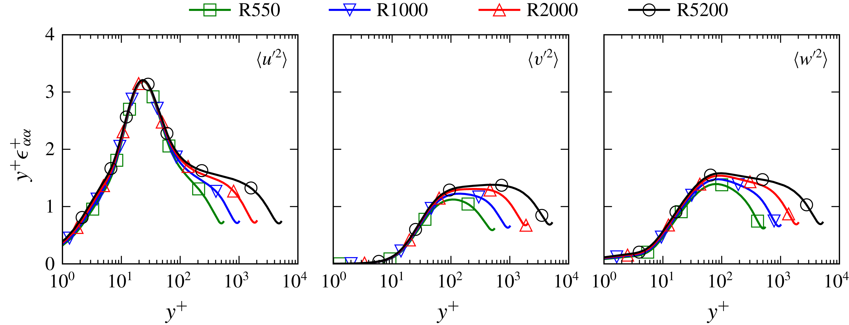
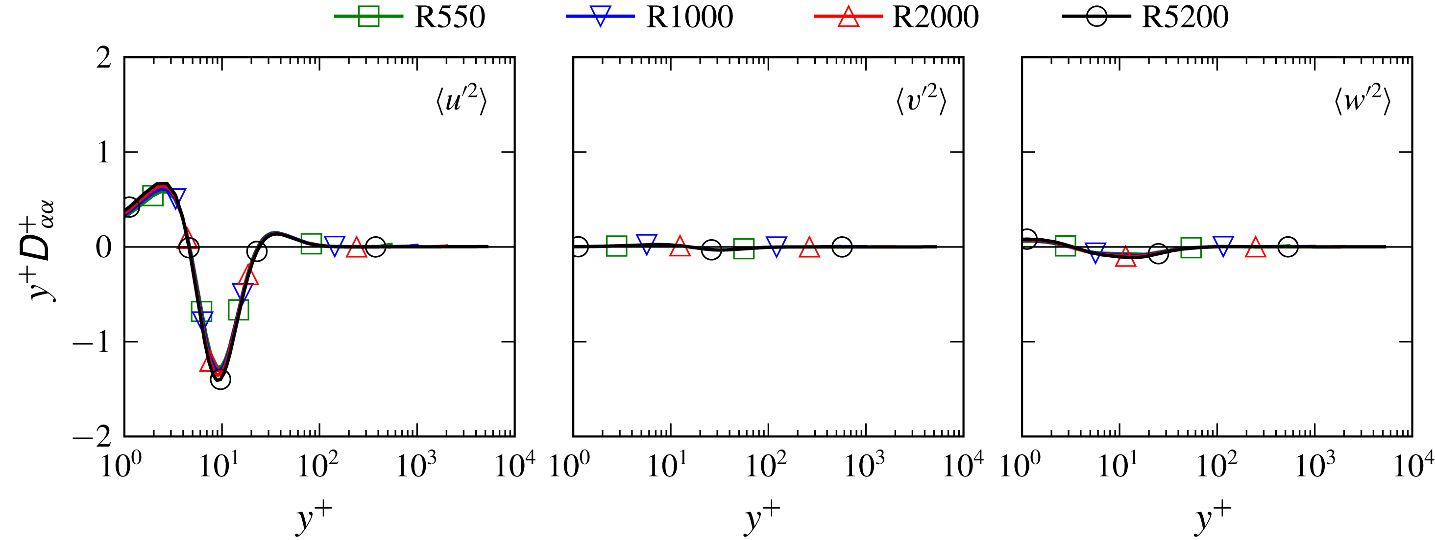
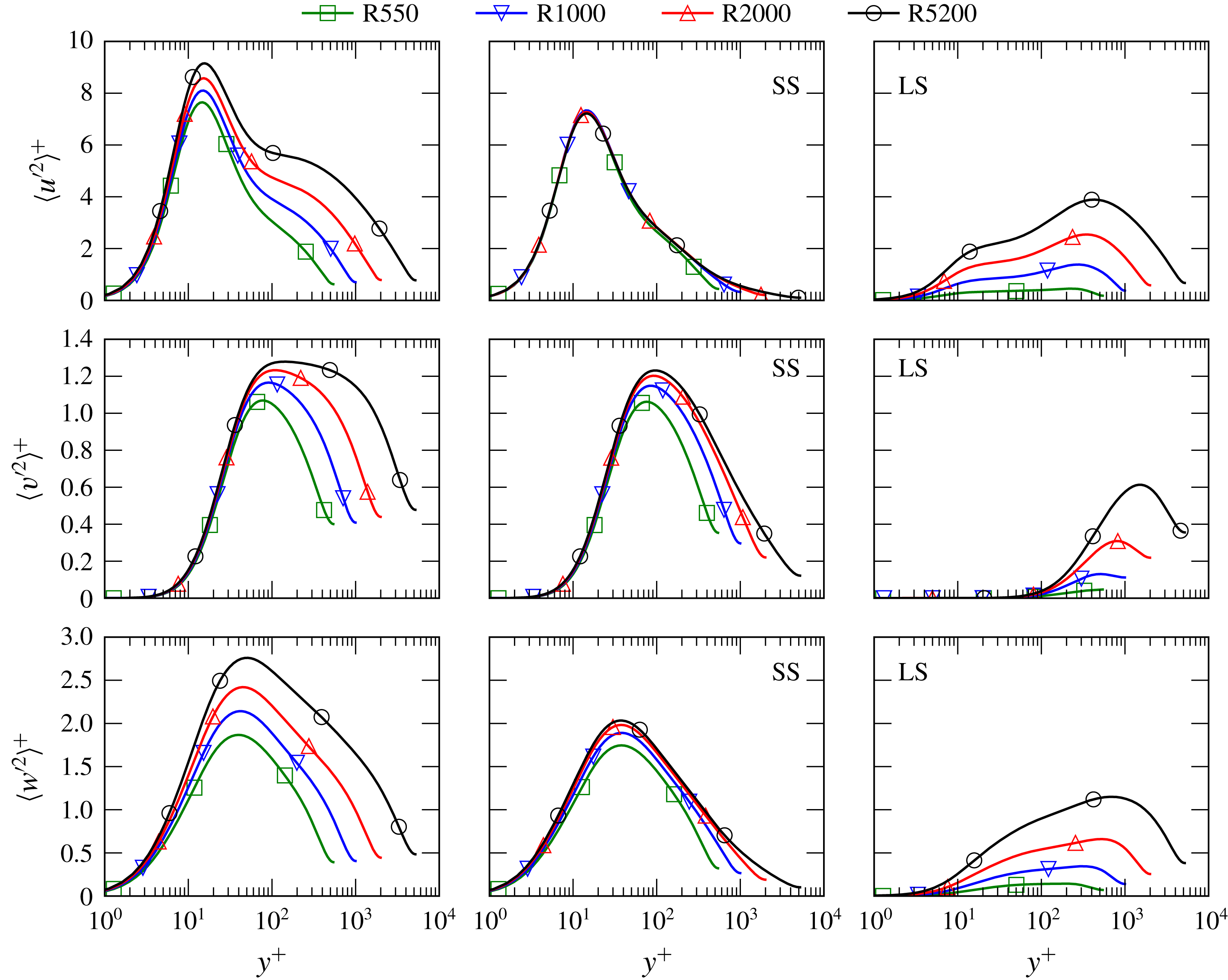
Profiles of
 $\langle u^{\prime 2}\rangle$
,
 $\langle v^{\prime 2}\rangle$
and
 $\langle w^{\prime 2}\rangle$
dissipation as log densities.

The one-dimensional profiles of the velocity variance dissipations are shown in figure 7. There are only weak
 $Re$
dependences in these profiles for
 $y^{+}<70$
. For
 $y^{+}>100$
or so and
 $y/\unicode[STIX]{x1D6FF}<0.2$
(the overlap region), all three dissipation profiles are approaching a plateau as
 $Re$
increases. This is as expected, under the assumptions of: (i) a constant stress region (
 $\langle u^{\prime }v^{\prime }\rangle ^{+}\approx -1$
) and logarithmic velocity profile in the overlap region, (ii) equality of production and dissipation of turbulent kinetic energy and (iii) isotropy of the dissipation. With these assumptions, the production and therefore dissipation of kinetic energy in the overlap region is given simply by
 $y^{+}\unicode[STIX]{x1D716}_{K}^{+}=1/\unicode[STIX]{x1D705}\approx 2.6$
, assuming
 $\unicode[STIX]{x1D705}=0.384$
as reported in Lee & Moser (Reference Lee and Moser2015a
). None of the above assumptions is exactly true. For example, a much higher Reynolds number is required for the Reynolds stress to approach one in the overlap region, and it appears that the equality of production and dissipation is an approximation that does not improve with increasing Reynolds number (Lee & Moser Reference Lee and Moser2015a
). Within these limitations, the profiles in figure 7 are in reasonable agreement with this prediction. For
 $y/\unicode[STIX]{x1D6FF}>0.2$
the premultiplied dissipation profiles of all components decrease for large
 $y$
, although at the centre of the channel they increase slightly. This increase is a consequence of multiplying the dissipation by
 $y$
since dissipation is symmetric and non-zero at the centre.
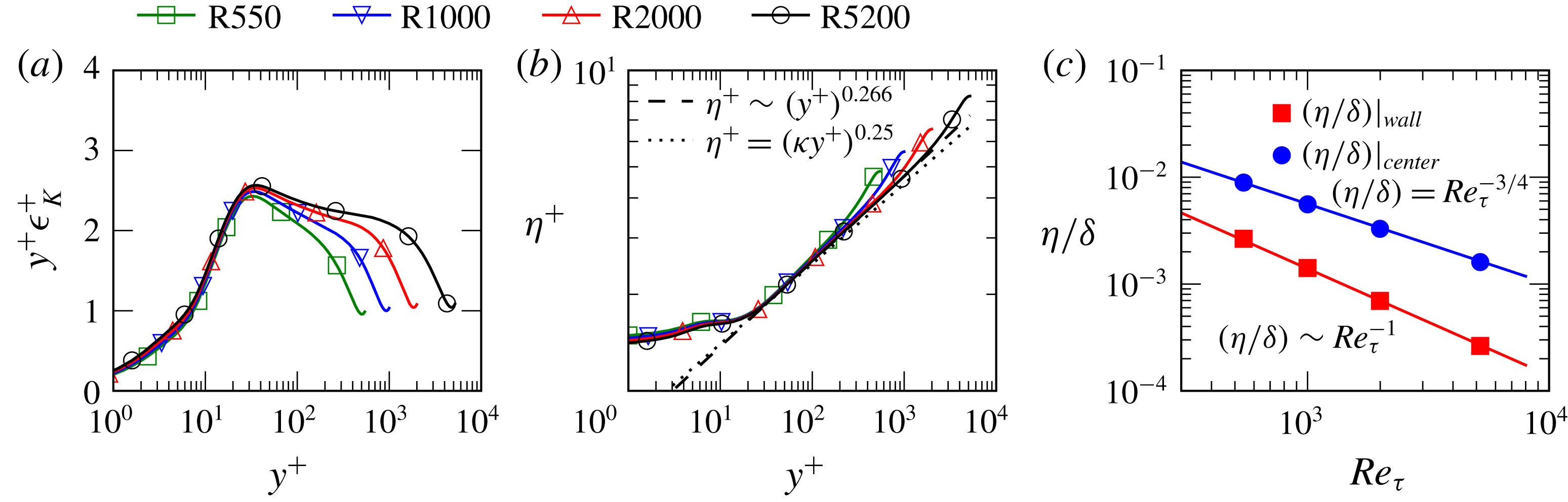
Profiles of kinetic energy dissipation
 $\unicode[STIX]{x1D716}_{K}$
(a) as log densities, and Kolmogorov length scale
 $\unicode[STIX]{x1D702}=(\unicode[STIX]{x1D708}^{3}/\unicode[STIX]{x1D716}_{K})^{1/4}$
(b) as a function of
 $y^{+}$
and (c)
 $\unicode[STIX]{x1D702}$
at the wall and channel centre as a function of Reynolds number.

The same assumptions also yield an estimate for the Kolmogorov length scale
 $\unicode[STIX]{x1D702}=(\unicode[STIX]{x1D708}^{3}/\unicode[STIX]{x1D716}_{k})^{1/4}$
(Tennekes & Lumley Reference Tennekes and Lumley1972). That is,
 $$\begin{eqnarray}\unicode[STIX]{x1D702}^{+}=(\unicode[STIX]{x1D716}_{K}^{+})^{-1/4}\approx (P_{K}^{+})^{-1/4}\approx (\unicode[STIX]{x1D705}y^{+})^{1/4}.\end{eqnarray}$$
Profiles of the dissipation of TKE and the Kolmogorov scale at different
 $Re$
are plotted in figure 8(a,b). In the overlap region, the
 $\unicode[STIX]{x1D702}$
profiles collapse reasonably well to a power-law dependence on
 $y^{+}$
, with an exponent of 0.266 which is only slightly different from
 $1/4$
. Again, a disagreement that is consistent with the limitations of the underlying assumptions. From figure 8(c), it is clear that
 $\unicode[STIX]{x1D702}/\unicode[STIX]{x1D6FF}$
scales as
 $Re_{\unicode[STIX]{x1D70F}}^{-1}$
and
 $Re_{\unicode[STIX]{x1D70F}}^{-3/4}$
at the wall and the centreline respectively, which is consistent with expectations from the law of the wall and Kolmogorov scaling.
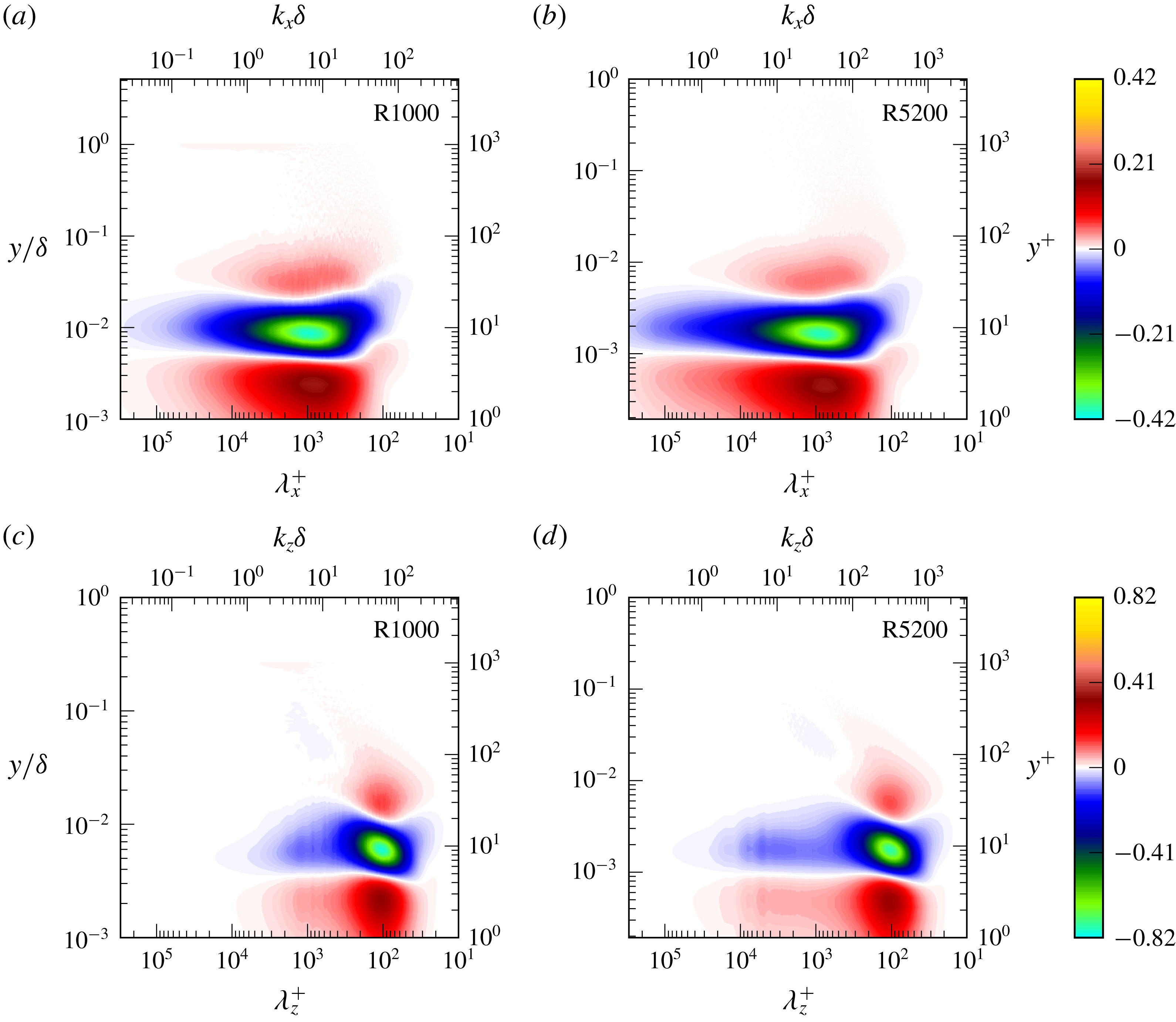
One-dimensional spectral density of
 $\langle u^{\prime 2}\rangle$
,
 $\langle v^{\prime 2}\rangle$
and
 $\langle w^{\prime 2}\rangle$
dissipation (a) in the streamwise direction and (b) in the spanwise direction: top of (a,b), R1000; bottom of (a,b), R5200. Solid lines are at
 $k_{x}y^{1/4}\unicode[STIX]{x1D6FF}^{3/4}=85$
, 130 and 130 (streamwise spectra) and
 $k_{z}y^{1/4}\unicode[STIX]{x1D6FF}^{3/4}=130$
, 130 and 85 (spanwise spectra) for
 $\langle u^{\prime 2}\rangle$
,
 $\langle v^{\prime 2}\rangle$
and
 $\langle w^{\prime 2}\rangle$
, respectively. The symbol
 $\times$
marks a feature discussed in the text.

The dissipation spectral densities from R1000 and R5200 are shown in figure 9. In both cases, the
 $\langle u^{\prime 2}\rangle$
dissipation spectra,
 $\unicode[STIX]{x1D60C}_{11}^{\unicode[STIX]{x1D716}}$
, have peaks at
 $y^{+}\approx 20$
,
 $\unicode[STIX]{x1D706}_{x}^{+}\approx 200$
and
 $\unicode[STIX]{x1D706}_{z}^{+}\approx 70$
. Notice that very close to the wall (
 $y^{+}<5$
), the streamwise
 $\langle u^{\prime 2}\rangle$
dissipation spectrum has a relatively broad high wavenumber peak, while the spanwise spectral peak in this region is narrower and centred around
 $\unicode[STIX]{x1D706}_{z}^{+}\approx 100$
. This is consistent with dissipation of the near-wall streaks due to the no-slip condition at the wall. Further, notice that near the wall, the spectral range of
 $\langle u^{\prime 2}\rangle$
dissipation extends to higher
 $\unicode[STIX]{x1D706}^{+}$
(larger scales) with increasing
 $Re$
, up to
 $\unicode[STIX]{x1D706}_{x}^{+}\sim 10^{5}$
and
 $\unicode[STIX]{x1D706}_{z}^{+}\sim 10^{4}$
at
 $Re_{\unicode[STIX]{x1D70F}}=5200$
. This is presumably due to the impact of the increasingly large (in ‘
 $+$
’ units) streamwise-elongated outer scales on the wall region, consistent with Jiménez (Reference Jiménez2012).
As is apparent in figure 7, the
 $\langle v^{\prime 2}\rangle$
dissipation is negligible near the wall because the wall-normal gradient of
 $v^{\prime }$
and thus the dissipation must be zero at the wall, and this is reflected in the spectra,
 $\unicode[STIX]{x1D60C}_{22}^{\unicode[STIX]{x1D716}}$
. The profiles of
 $\langle w^{\prime 2}\rangle$
dissipation are similar to those for
 $\langle v^{\prime 2}\rangle$
, with the exception of near the wall (
 $y^{+}<10$
), since
 $\langle w^{\prime 2}\rangle$
dissipation is not zero at the wall. The spectra (
 $\unicode[STIX]{x1D60C}_{22}^{\unicode[STIX]{x1D716}}$
and
 $\unicode[STIX]{x1D60C}_{33}^{\unicode[STIX]{x1D716}}$
) are also similar, with the most obvious difference being a weak region of
 $\langle w^{\prime 2}\rangle$
dissipation around
 $y^{+}=20$
and
 $\unicode[STIX]{x1D706}_{x}^{+}=200$
(marked with
 $\times$
) that roughly overlaps the region where
 $E_{11}^{\unicode[STIX]{x1D716}}$
has its strong peak. These near-wall dissipation spectra are consistent with the known structure of near-wall turbulence, particularly the presence of streamwise vortices with limited streamwise extent.
In the overlap region, the location of the dissipation spectral peak of all three components varies as approximately
 $\unicode[STIX]{x1D706}\sim y^{1/4}$
(see the solid lines in figure 9). This is consistent with the observation above (3.3) that the Kolmogorov scale varies approximately like
 $y^{1/4}$
.
Two-dimensional spectral density of
 $\langle u^{\prime 2}\rangle$
,
 $\langle v^{\prime 2}\rangle$
and
 $\langle w^{\prime 2}\rangle$
dissipation in log-polar coordinates, as defined in figure 1, from R5200;
 $\unicode[STIX]{x1D706}^{+}=10$
on the outermost dotted circle and increases by a factor of 10 for each dotted circle moving inward. The arrow in the
 $\langle u^{\prime 2}\rangle$
spectrum at
 $y^{+}=3$
marks a feature discussed in the text.

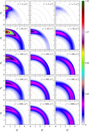
The two-dimensional dissipation spectra in figure 10 provide more detailed information regarding the dissipation scales. Very near the wall (
 $y^{+}=3$
), the spectrum has the same structure as the near-wall velocity spectra (see figure 2), which is as expected because the dissipation this close to the wall is dominated by the wall-normal derivatives (Antonia, Kim & Browne Reference Antonia, Kim and Browne1991), and the velocity is zero at the wall. Note particularly that even the large-scale spectral peaks along the
 $k_{z}^{\#}$
axis as described for the
 $\langle u^{\prime 2}\rangle$
spectra (see § 3.1) are present in the
 $\langle u^{\prime 2}\rangle$
dissipation spectrum for this reason (marked with an arrow). With increasing distance from the wall, the dissipation occurs more isotropically in scale, in a band of modes with wavelengths that increase slowly with
 $y$
(like
 $y^{1/4}$
), consistent with the structure of the one-dimensional dissipation spectra. By
 $y^{+}=1000$
, the
 $\langle v^{\prime 2}\rangle$
dissipation spectrum is nearly isotropic in scale, but the
 $\langle u^{\prime 2}\rangle$
and
 $\langle w^{\prime 2}\rangle$
spectra do not appear to be. However, this is simply due to the difference in contributions between longitudinal and transverse derivatives to the dissipation, because of continuity. In particular, in isotropic turbulence, the variance of the longitudinal derivatives is half that of the transverse derivatives. The stronger
 $\langle u^{\prime 2}\rangle$
(
 $\langle w^{\prime 2}\rangle$
) dissipation spectra along the
 $k_{z}^{\#}$
(
 $k_{x}^{\#}$
) axis is consistent with this characteristic of isotropic turbulence.
It appears then that the dissipation processes are anisotropic near the wall and become isotopic in scale as
 $y$
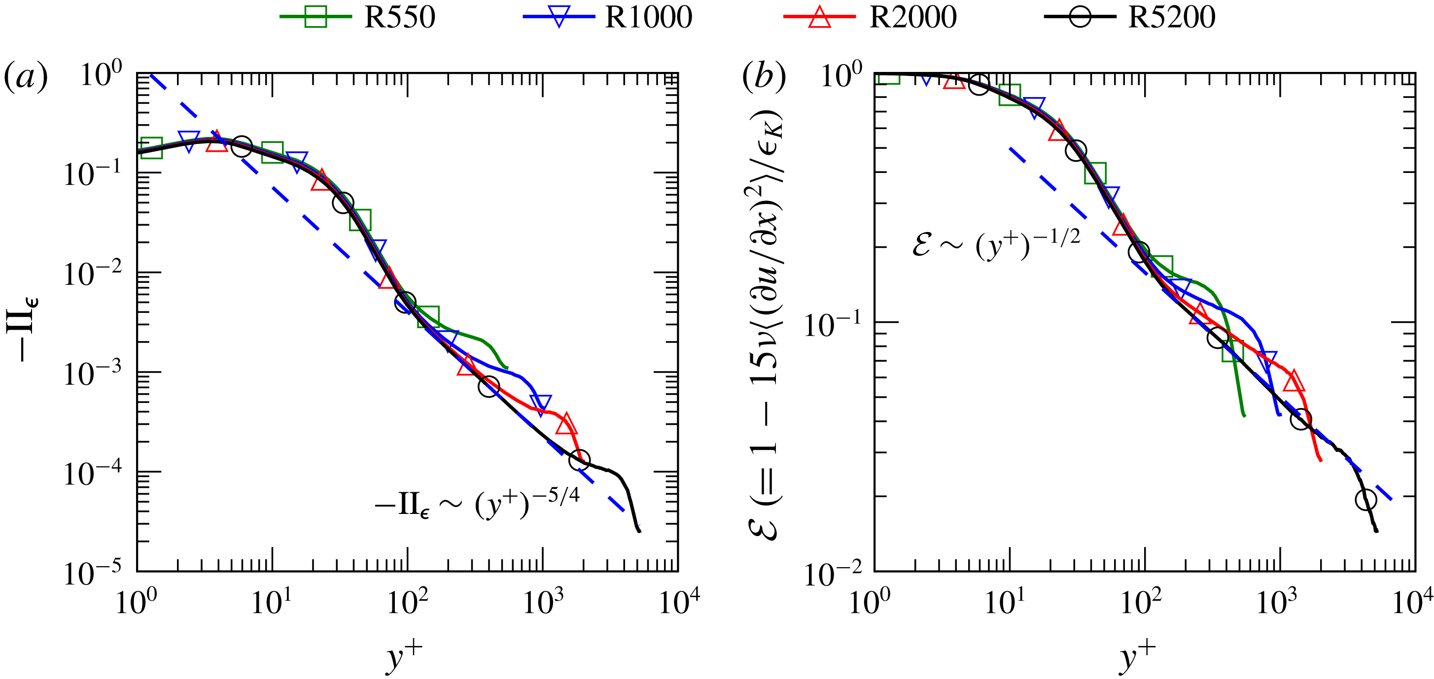
increases. Anisotropy is expected near the wall because of the presence of the wall, and local isotropy is widely assumed in modelling wall-bounded flow away from the wall. To characterise the component anisotropy of the dissipation, the second invariant of the deviatoric part of the dissipation tensor,
 $\text{II}_{\unicode[STIX]{x1D750}}$
, is computed as suggested by Antonia et al. (Reference Antonia, Kim and Browne1991) and Antonia, Djenidi & Spalart (Reference Antonia, Djenidi and Spalart1994):
 $$\begin{eqnarray}\text{II}_{\unicode[STIX]{x1D750}}=-\frac{1}{2}\unicode[STIX]{x1D625}_{ij}\unicode[STIX]{x1D625}_{ji}\quad \text{with }\unicode[STIX]{x1D625}_{ij}=\frac{\unicode[STIX]{x1D716}_{ij}}{2\unicode[STIX]{x1D716}_{K}}-\frac{\unicode[STIX]{x1D6FF}_{ij}}{3}.\end{eqnarray}$$
Also of interest is the error committed when using an assumption of isotropy in both scale and components to estimate the dissipation of kinetic energy from the variance of
 $\unicode[STIX]{x2202}u/\unicode[STIX]{x2202}x$
, as might be done with experimental data. These characterisations of anisotropy are shown as a function of
 $y^{+}$
in figure 11(a,b). As expected, anisotropy of dissipation decreases with distance from the wall. In particular, in the overlap region (
 $y^{+}\approx 100$
to
 $y/\unicode[STIX]{x1D6FF}\approx 0.2$
)
 $\text{II}_{\unicode[STIX]{x1D750}}$
varies as
 $-y^{-5/4}$
while the relative error in estimating dissipation from the streamwise velocity gradient varies like
 $y^{-1/2}$
.
Isotropy of dissipation: (a) second invariant of the deviatoric part of the dissipation tensor; and (b) relative error of estimating the dissipation from the variance of
 $\unicode[STIX]{x2202}u/\unicode[STIX]{x2202}x$
using isotropy.

3.4 Inter-component energy transfer
The pressure–strain correlation
 $\unicode[STIX]{x1D72B}^{s}$
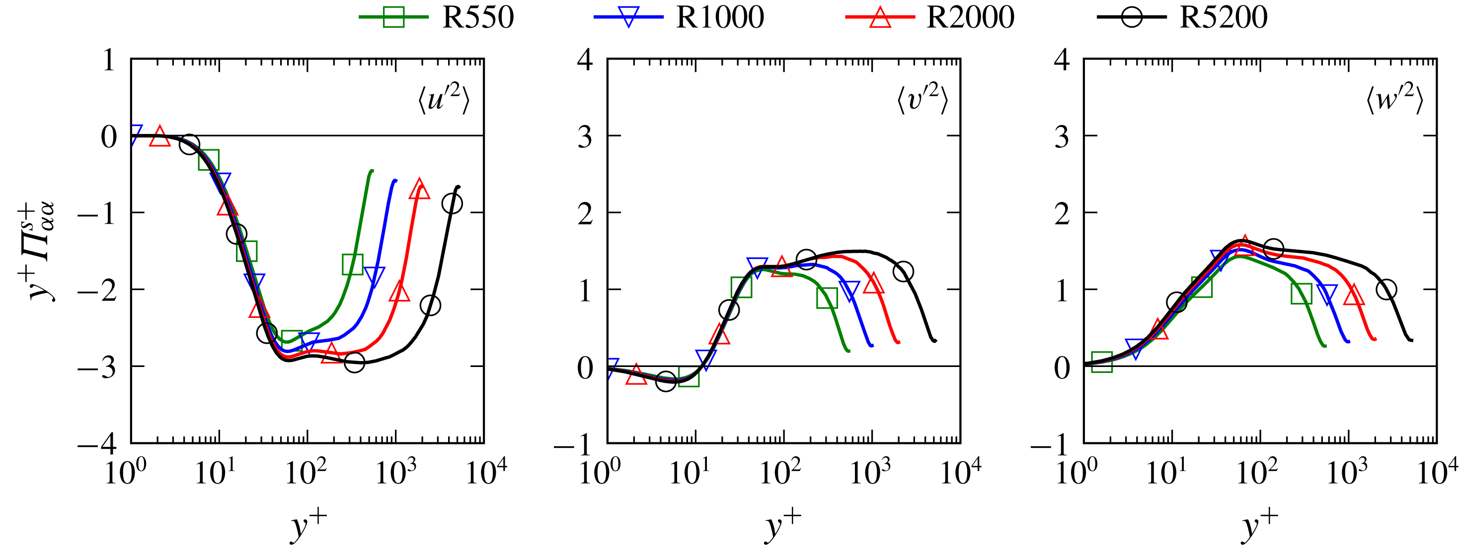
exchanges energy between the velocity components (it has zero trace). As is well known, energy production occurs only in
 $\langle u^{\prime 2}\rangle$
but the dissipation occurs in all three components, and
 $\unicode[STIX]{x1D72B}^{s}$
enables this by redistributing energy from
 $\langle u^{\prime 2}\rangle$
to the other components. This is shown in figure 12, where the streamwise component
 $\unicode[STIX]{x1D6F1}_{11}^{s}$
is negative except for
 $y^{+}<1.5$
, where it is only slightly positive, while the
 $\unicode[STIX]{x1D6F1}_{22}^{s}$
and
 $\unicode[STIX]{x1D6F1}_{33}^{s}$
components are positive almost everywhere. The one exception is that
 $\unicode[STIX]{x1D6F1}_{22}^{s}$
is negative for
 $y^{+}<12$
. This is due to the well-known ‘splat’ effect (Mansour et al.
Reference Mansour, Kim and Moin1988; Perot & Moin Reference Perot and Moin1995), in which fluid moving toward the wall is blocked by the wall and must turn to flow parallel to the wall, transferring energy from the vertical to horizontal velocity fluctuations. Because vertical velocity fluctuations very near the wall are primarily associated with streamwise vortices, this energy transfer is primarily from
 $\langle v^{\prime 2}\rangle$
to
 $\langle w^{\prime 2}\rangle$
.
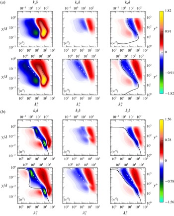
Profiles of the pressure strain terms for
 $\langle u^{\prime 2}\rangle$
,
 $\langle v^{\prime 2}\rangle$
and
 $\langle w^{\prime 2}\rangle$
, as log densities.

It is interesting to note that in the components parallel to the wall (
 $\unicode[STIX]{x1D6F1}_{11}^{s}$
and
 $\unicode[STIX]{x1D6F1}_{33}^{s}$
), there is a weak Reynolds number dependence in the profiles near the wall, while the profile of the wall-normal component (
 $\unicode[STIX]{x1D6F1}_{22}^{s}$
) is Reynolds number independent out to
 $y^{+}$
as large as 100. This is presumably because there are processes in the near-wall exchange of energy between
 $\langle u^{\prime 2}\rangle$
and
 $\langle w^{\prime 2}\rangle$
that are mediated by outer region turbulent structures that do not involve
 $\langle v^{\prime 2}\rangle$
. Also interesting is that a broad outer peak in the profiles appears to develop with increasing Reynolds number, in both the streamwise and wall-normal components (
 $\unicode[STIX]{x1D6F1}_{11}^{s}$
and
 $\unicode[STIX]{x1D6F1}_{22}^{s}$
) at
 $y/\unicode[STIX]{x1D6FF}\approx 0.1$
and 0.2 respectively. These are in the outer parts of the overlap region. However, no such outer peak seems to be developing in the spanwise component. These differences suggest that the mechanisms for exchange of energy to
 $\langle v^{\prime 2}\rangle$
and
 $\langle w^{\prime 2}\rangle$
are different.
One-dimensional spectral density of the
 $\langle u^{\prime 2}\rangle$
,
 $\langle v^{\prime 2}\rangle$
and
 $\langle w^{\prime 2}\rangle$
pressure–strain terms (a) in the streamwise direction and (b) in the spanwise direction: top of (a,b), R1000; bottom of (a,b), R5200. Solid lines are at
 $ky=2.5$
. Dashed lines in streamwise spectra are at
 $k_{x}y=0.1$
.

Two-dimensional spectral density of the
 $\langle u^{\prime 2}\rangle$
,
 $\langle v^{\prime 2}\rangle$
and
 $\langle w^{\prime 2}\rangle$
pressure–strain terms in log-polar coordinates as defined in figure 1, from R5200;
 $\unicode[STIX]{x1D706}^{+}=10$
on the outermost dotted circle and increases by a factor of 10 for each dotted circle moving inward. Symbols (
 $\times$
and
 $\star$
) mark features discussed in the text.

Just as the pressure–strain term in the two-point correlation has zero trace (2.12), so does the pressure–strain spectrum:
 $$\begin{eqnarray}\unicode[STIX]{x1D60C}_{ii}^{\unicode[STIX]{x1D6F1}^{s}}=0\quad \forall \;(k_{x},y,k_{z}).\end{eqnarray}$$
Thus, the one- and two-dimensional pressure–strain spectra can be interpreted as inter-component energy transfer at given scales (wavenumbers) and wall-normal locations. The one-dimensional spectra of the pressure strain terms are shown in figure 13. The dominant feature of these spectra, for both Reynolds numbers and in both spectral directions (
 $k_{x}$
and
 $k_{z}$
), is a transfer of energy from
 $\langle u^{\prime 2}\rangle$
to
 $\langle v^{\prime 2}\rangle$
and
 $\langle w^{\prime 2}\rangle$
over a range of wavenumbers that scale with
 $y^{-1}$
. This feature, which extends from
 $y^{+}\approx 30$
to
 $y/\unicode[STIX]{x1D6FF}\approx 0.5$
, is centred on the high wavenumber side of the region of
 $\langle u^{\prime 2}\rangle$
production (see figure 5) in
 $k_{x}$
, and is centred on the maximum production region in
 $k_{z}$
. Indeed over this range in
 $y$
, the pressure–strain spectral peaks of
 $\langle u^{\prime 2}\rangle$
occur at
 $k_{x}y\approx k_{z}y\approx 2.5$
, while the production peaks occur at
 $k_{x}y\approx 0.5$
and
 $k_{z}y\approx 2$
, with significant production occurring at wavenumbers as low as
 $k_{x}y\approx 0.06$
. There is thus a range of large scales (low wavenumbers) in
 $x$
at which there is significant production of
 $\langle u^{\prime 2}\rangle$
and insignificant transfer of energy to the other components. The same is true near the wall, where
 $\langle u^{\prime 2}\rangle$
production at scales that are long in
 $x$
results in no transfer to other components. This low
 $x$
-wavenumber production occurs with much higher
 $z$
-wavenumbers, as is clear from figure 6. The production of streamwise velocity fluctuations that are elongated in
 $x$
in this way will not significantly impact continuity, and will therefore not generate a significant pressure response or inter-component transfer. This suggests that pressure redistribution should be dominated by wavenumbers with
 $k_{x}$
of the same order as
 $k_{z}$
, which is consistent with the one-dimensional spectra in figure 13, although the two-dimensional spectra indicate that things are a bit more complex, especially near the wall.
Another noteworthy feature of the one-dimensional spectra is the weakly negative region in the streamwise spectrum of
 $\unicode[STIX]{x1D6F1}_{33}^{s}$
that extends from the centre of the channel to
 $y^{+}\approx 30$
(marked with a dashed line in figure 13). This energy is transferred to
 $\langle v^{\prime 2}\rangle$
, as indicated by the fact that there is a corresponding positive region in the
 $\unicode[STIX]{x1D6F1}_{22}^{s}$
spectrum (also marked with a dashed line), but not
 $\unicode[STIX]{x1D6F1}_{11}^{s}$
. It appears that the source of the
 $\langle w^{\prime 2}\rangle$
energy at these wavenumbers is inter-scale transfer from the dominant positive region in figure 13 to larger scales (see discussion in § 3.6).
Two-dimensional pressure–strain spectra at several
 $y$
-locations are shown in figure 14. One common feature of the spectra at all
 $y$
-locations is that the dominant inter-component transfer occurs in a circular band of wavenumbers centred around a value of
 $k$
that increases with
 $y$
. Beyond
 $y^{+}\approx 300$
, the dominant wavelength scales with
 $y$
, with the centre of the dominant zone at
 $ky\approx 2.5$
, consistent with the one-dimensional spectra. The width of the dominant zone also increases with
 $y$
, presumably because of the increase in local Reynolds number. Another common feature is that at the
 $k_{x}^{\#}=0$
and
 $k_{z}^{\#}=0$
axes, the
 $\unicode[STIX]{x1D6F1}_{11}^{s}$
and
 $\unicode[STIX]{x1D6F1}_{33}^{s}$
spectra, respectively, go to zero. This is because for modes with no variation in
 $x$
(
 $z$
) the fluctuations in
 $u$
(
 $w$
) have no impact on continuity, and so do not produce a pressure response.
Very near the wall (
 $y^{+}=3$
in figure 14), the spectra are dominated by the splat effect discussed above. Here, the energy is primarily transferred from
 $\langle v^{\prime 2}\rangle$
to
 $\langle w^{\prime 2}\rangle$
for fluctuations that are strongly aligned in the streamwise direction, with the strongest transfers occurring at
 $k_{x}=0$
. Curiously there is also a weak transfer from
 $\langle u^{\prime 2}\rangle$
to
 $\langle w^{\prime 2}\rangle$
in these streamwise-elongated wavenumbers. Wavenumbers associated with spanwise elongation also produce transfers, but in this case from
 $\langle v^{\prime 2}\rangle$
to
 $\langle u^{\prime 2}\rangle$
. This is consistent with expectations for elongated regions of motion toward the wall, that the fluid turns in the direction perpendicular to the elongation, like a two-dimensional stagnation point flow.
Except for very near the wall (
 $y^{+}=3$
), the dominant transfer is from
 $\langle u^{\prime 2}\rangle$
to
 $\langle v^{\prime 2}\rangle$
and
 $\langle w^{\prime 2}\rangle$
over a broad range of wavenumber orientations centred around
 $k_{x}\approx k_{z}$
farther from the wall (
 $y^{+}=300$
and 1000), and centred around a more streamwise-elongated orientation (
 $k_{z}\approx 2k_{x}$
) at
 $y^{+}=30$
(see dashed guide lines in figure 14). This transfer is strongest to
 $\langle w^{\prime 2}\rangle$
, except for the spanwise-elongated modes (
 $k_{z}$
near zero). In addition, except very near the wall, there is a strong transfer from
 $\langle w^{\prime 2}\rangle$
to
 $\langle v^{\prime 2}\rangle$
where
 $k_{z}\gg k_{x}$
(marked with
 $\times$
) as well as transfer from
 $\langle v^{\prime 2}\rangle$
to
 $\langle w^{\prime 2}\rangle$
at larger scales (smaller
 $k_{z}^{\#}$
, marked with
 $\star$
). Transfer between
 $\langle v^{\prime 2}\rangle$
and
 $\langle w^{\prime 2}\rangle$
like this would be expected from streamwise oriented vortices. It is this structure that is responsible for the negative regions in figure 13. It is also interesting that there is weak transfer from
 $\langle v^{\prime 2}\rangle$
to
 $\langle u^{\prime 2}\rangle$
and
 $\langle w^{\prime 2}\rangle$
even away from the wall (
 $y^{+}=30$
and 300) for
 $\unicode[STIX]{x1D706}^{+}\gg y^{+}$
. As with the splat effect the transfer is toward
 $\langle u^{\prime 2}\rangle$
(
 $\langle w^{\prime 2}\rangle$
) for modes that are elongated in
 $z$
(
 $x$
). Indeed, for such large wavelength modes, even these
 $y$
-locations are essentially ‘close’ to the wall, so it may indeed be a manifestation of the splat effect.
The scale-dependent inter-component transfer described here is complicated, with only the near-wall process described in terms of the structural features of the turbulence. We should aspire to conceptual models of wall-bounded turbulence in the buffer and overlap regions that are consistent with these observations.
3.5 Wall-normal energy transport
As is well known, there are two wall-normal energy transport mechanisms: a linear mechanism due to viscous diffusion, and a nonlinear mechanism due to turbulent fluctuations. These linear and nonlinear transport mechanisms are investigated in the following subsections.
3.5.1 Linear mechanism: viscous diffusion
Profiles of
 $\langle u^{\prime 2}\rangle$
,
 $\langle v^{\prime 2}\rangle$
and
 $\langle w^{\prime 2}\rangle$
viscous transport as log densities.

One-dimensional streamwise and spanwise spectral densities of
 $\unicode[STIX]{x1D60B}_{11}$
.

Two-dimensional spectral density of
 $D_{11}$
in log-polar coordinates, as defined in figure 1, at
 $y^{+}=15$
;
 $\unicode[STIX]{x1D706}^{+}=10$
on the outermost dotted circle and increases by a factor of 10 for each dotted circle moving inward. The arrow marks a feature discussed in the text.

The one-dimensional profile of viscous transport in the
 $y$
direction is shown in figure 15. The transport of
 $\langle v^{\prime 2}\rangle$
and
 $\langle w^{\prime 2}\rangle$
is negligible compared to the viscous transport of
 $\langle u^{\prime 2}\rangle$
. There is a weak
 $Re$
dependence in
 $\unicode[STIX]{x1D60B}_{11}^{+}$
near the wall (
 $y^{+}<100$
), which is absent further from the wall. This weak
 $Re$
dependence can be understood in the context of the one-dimensional diffusion spectra, which are shown in figure 16. The dominant small-scale structure of these spectra appears the same at the two Reynolds numbers shown. For both Reynolds numbers, the spectral peaks occur at approximately
 $\unicode[STIX]{x1D706}_{x}^{+}\approx 800$
and
 $\unicode[STIX]{x1D706}_{z}^{+}\approx 100$
. However, the contribution from the large scales increases with
 $Re$
. There even appear to be weak large-scale local extrema at
 $k_{z}\unicode[STIX]{x1D6FF}\approx 7$
in the spanwise spectra at
 $y^{+}\approx 3$
and
 $y^{+}\approx 10$
although it is not obvious in figure 16.
The reason for the Reynolds number dependence is clearer in the two-dimensional
 $\unicode[STIX]{x1D60B}_{11}$
spectra at
 $y^{+}=15$
shown in figure 17 for flows at different Reynolds numbers. These spectra have the same structure as the
 $\langle u^{\prime 2}\rangle$
spectra at the same
 $y$
-location and Reynolds numbers in figure 3, except that here the spectrum is negative because this
 $y$
-location is near the negative peak of the
 $\langle u^{\prime 2}\rangle$
transport in figure 15. The structural similarity includes the large wavelength region of large magnitude along the
 $k_{z}^{\#}$
axis, which is the primary feature that depends on Reynolds number (marked with an arrow). As discussed in § 3.1, this spectral region arises due to large-scale outer flow structures that are imposed on the near-wall turbulence, which also explains the Reynolds number dependence. A quantitative analysis of the effects of these large-scale features on Reynolds number dependence is provided in § 3.7.
3.5.2 Nonlinear mechanism: turbulent and pressure-driven wall-normal transport
Profile of
 $\langle u^{\prime 2}\rangle$
,
 $\langle v^{\prime 2}\rangle$
and
 $\langle w^{\prime 2}\rangle$
nonlinear transport, as log densities and the nonlinear flux
 $\unicode[STIX]{x1D6F7}_{\unicode[STIX]{x1D6FC}\unicode[STIX]{x1D6FC}}$
as defined in (3.6).

The other wall-normal transport mechanism is nonlinear, resulting from the action of turbulent fluid motions. As discussed in § 2, the nonlinear transport term
 ${\mathcal{N}}_{ij}=\unicode[STIX]{x1D61B}_{ij}^{\bot }+\unicode[STIX]{x1D6F1}_{ij}^{d}$
is the combination of the usual turbulent transport and pressure transport terms, which we will consider here first. It was shown in Lee & Moser (Reference Lee and Moser2015a
) that the difference between production and dissipation is
 $Re$
dependent for
 $y^{+}\gtrsim 70$
. As we saw in § 3.5.1 viscous transport terms do not have a significant
 $Re$
dependence, so the nonlinear transport term must be
 $Re$
-dependent in the outer region to balance the production/dissipation mismatch.
The one-dimensional profiles of nonlinear transport are shown in figure 18. As with the other terms examined here, only modest
 $Re$
dependences are observed near the wall, particularly the slow increase of the near-wall peak of
 $y^{+}{\mathcal{N}}_{11}$
(
 $=y^{+}T_{11}^{+}$
) with
 $Re$
. However, further from the wall (
 $y^{+}\gtrsim 100$
), the turbulent transport of
 $\langle u^{\prime 2}\rangle$
(
 ${\mathcal{N}}_{11}$
) decreases with increasing
 $Re$
where negative
 ${\mathcal{N}}_{\unicode[STIX]{x1D6FC}\unicode[STIX]{x1D6FC}}$
implies a net transport of energy from this region to other region(s). The local minimum of
 $y^{+}{\mathcal{N}}_{11}^{+}$
in the R5200 case occurs at
 $y^{+}\approx 300$
. Beyond this local minimum,
 $y^{+}{\mathcal{N}}_{11}^{+}$
increases logarithmically when
 $Re_{\unicode[STIX]{x1D70F}}\gtrsim 2000$
, as shown in figure 18, and the slope appears to be independent of
 $Re$
. This logarithmic dependence ends at
 $y/\unicode[STIX]{x1D6FF}\approx 0.6$
, where
 $y^{+}{\mathcal{N}}_{11}^{+}$
increases much more rapidly.
Unlike
 $y^{+}{\mathcal{N}}_{11}^{+}$
, the
 $y^{+}{\mathcal{N}}_{22}^{+}$
and
 $y^{+}{\mathcal{N}}_{33}^{+}$
profiles do not exhibit significant
 $Re$
dependences. The transport of
 $\langle v^{\prime 2}\rangle$
by
 ${\mathcal{N}}_{22}$
is primarily from the region where
 $y^{+}\gtrsim 15$
and
 $y/\unicode[STIX]{x1D6FF}\lesssim 0.6$
to the near-wall region and the region around the channel centreline. The transport by
 ${\mathcal{N}}_{33}$
is weaker, with energy transported from regions around
 $y^{+}=10$
and
 $y^{+}=50$
to the outer region (
 $y/\unicode[STIX]{x1D6FF}\gtrsim 0.3$
). Note that both
 $T_{22}^{\bot }$
and
 ${\mathcal{N}}_{33}$
are nearly zero in the region from
 $y^{+}\approx 200$
to
 $y/\unicode[STIX]{x1D6FF}\approx 0.3$
. Hence
 $\langle v^{\prime 2}\rangle$
energy is only deposited in this region by pressure transport and
 $\langle w^{\prime 2}\rangle$
energy is transported through this region without impacting the local balance of
 $\langle w^{\prime 2}\rangle$
.
The rather complex structures of
 ${\mathcal{N}}_{11}$
and
 ${\mathcal{N}}_{22}$
, raises the question of the direction of the net transport of
 $\langle u^{\prime 2}\rangle$
and
 $\langle v^{\prime 2}\rangle$
. To determine this, the net flux of energy
 $\unicode[STIX]{x1D6F7}_{\unicode[STIX]{x1D6FC}\unicode[STIX]{x1D6FC}}$
due to
 ${\mathcal{N}}_{\unicode[STIX]{x1D6FC}\unicode[STIX]{x1D6FC}}$
was computed, where
 $$\begin{eqnarray}\unicode[STIX]{x1D6F7}_{\unicode[STIX]{x1D6FC}\unicode[STIX]{x1D6FC}}(y)=\int _{0}^{y}{\mathcal{N}}_{\unicode[STIX]{x1D6FC}\unicode[STIX]{x1D6FC}}(Y)\,\text{d}Y=-\langle u_{\unicode[STIX]{x1D6FC}}^{\prime }u_{\unicode[STIX]{x1D6FC}}^{\prime }v^{\prime }\rangle (y)+\langle u_{2}^{\prime }p^{\prime }\unicode[STIX]{x1D6FF}_{2\unicode[STIX]{x1D6FC}}\rangle (y).\end{eqnarray}$$
With this definition, positive
 $\unicode[STIX]{x1D6F7}_{\unicode[STIX]{x1D6FC}\unicode[STIX]{x1D6FC}}$
signifies flux toward the wall. The profiles of
 $\unicode[STIX]{x1D6F7}_{\unicode[STIX]{x1D6FC}\unicode[STIX]{x1D6FC}}$
are shown in figure 18. It is obvious that
 $\unicode[STIX]{x1D6F7}_{\unicode[STIX]{x1D6FC}\unicode[STIX]{x1D6FC}}$
must be zero at the wall and the centre of the channel because of the boundary conditions and statistical symmetry. In all cases,
 $\unicode[STIX]{x1D6F7}_{11}$
is zero at
 $y^{+}\approx 15$
, which is where
 $y^{+}{\mathcal{N}}_{11}^{+}$
has a local minimum. Thus, in all cases, the net flux of
 $\langle u^{\prime 2}\rangle$
is toward the wall for
 $y^{+}\lesssim 15$
and away from the wall at larger
 $y^{+}$
. In all cases,
 $\unicode[STIX]{x1D6F7}_{22}$
is zero at
 $y/\unicode[STIX]{x1D6FF}\approx 0.2$
, indicating that
 $\langle v^{\prime 2}\rangle$
energy is transported toward the wall in this region. On the other hand,
 $\langle w^{\prime 2}\rangle$
energy is transported away from the wall throughout the channel.
Note that there is a local maximum in
 $\unicode[STIX]{x1D6F7}_{11}$
at
 $y^{+}\approx 100$
, which is obviously just the point where
 ${\mathcal{N}}_{11}$
changes sign. But, the value of
 $\unicode[STIX]{x1D6F7}_{11}$
at the local maximum is getting larger (less negative) with increasing
 $Re$
. The reason is the growth with
 $Re$
of the near-wall peak in
 ${\mathcal{N}}_{11}$
. If this trend continues, at high enough
 $Re$
this local maximum will exceed zero, introducing another region in which the net flux is toward the wall. This complex structure of the turbulent transport is an aggregation of transport occurring at all scales. A better understanding requires a spectral analysis.
In § 2, we showed that the turbulent convection of the two-point correlation can be decomposed into terms representing transport in the wall-normal direction and scale transfer in wall-parallel directions (see (2.5)). The two-dimensional spectra of these terms are just their Fourier transforms, and they inherit the properties of the decomposition, such as (2.6) and (2.7). The turbulent convection spectrum
 $\unicode[STIX]{x1D60C}_{ij}^{T}$
, which is the Fourier transform of
 $\unicode[STIX]{x1D619}_{ij}^{T}$
, is thus decomposed as
 $$\begin{eqnarray}\unicode[STIX]{x1D60C}_{ij}^{T}(k_{x},y,k_{z})=\unicode[STIX]{x1D60C}_{ij}^{T^{\Vert }}(k_{x},y,k_{z})+\unicode[STIX]{x1D60C}_{ij}^{T^{\bot }}(k_{x},y,k_{z}),\end{eqnarray}$$
where
 $\unicode[STIX]{x1D60C}_{ij}^{T^{\Vert }}$
and
 $\unicode[STIX]{x1D60C}_{ij}^{T^{\bot }}$
are the Fourier transforms of
 $\unicode[STIX]{x1D619}_{ij}^{T^{\Vert }}$
and
 $\unicode[STIX]{x1D619}_{ij}^{T^{\bot }}$
, respectively. Further,
 $\unicode[STIX]{x1D60C}_{ij}^{{\mathcal{N}}}=\unicode[STIX]{x1D60C}_{ij}^{T^{\bot }}+\unicode[STIX]{x1D60C}_{ij}^{\unicode[STIX]{x1D6F1}^{d}}$
is the Fourier transform of
 $\unicode[STIX]{x1D619}_{ij}^{{\mathcal{N}}}$
. The Fourier transforms satisfy
 $$\begin{eqnarray}\int _{0}^{\unicode[STIX]{x1D6FF}}\unicode[STIX]{x1D60C}_{ij}^{{\mathcal{N}}}(k_{x},y,k_{z})\,\text{d}y=0,\quad \forall (k_{x},k_{z}),\end{eqnarray}$$
and
 $$\begin{eqnarray}\iint _{0}^{\infty }\unicode[STIX]{x1D60C}_{ij}^{T^{\Vert }}(k_{x},y,k_{z})\,\text{d}k_{x}\,\text{d}k_{z}=0,\quad \forall y.\end{eqnarray}$$
Hence, we can interpret
 $\unicode[STIX]{x1D60C}_{ij}^{{\mathcal{N}}}$
as nonlinear transport in the wall-normal direction at each scale defined by the wavenumbers
 $(k_{x},k_{z})$
, and interpret
 $\unicode[STIX]{x1D60C}_{ij}^{T^{\Vert }}$
as the transfer in scale in the wall-parallel directions at each wall-normal location
 $y$
. Further, the property (3.8b
) implies that
 $$\begin{eqnarray}\iint _{0}^{\infty }\unicode[STIX]{x1D60C}_{ij}^{{\mathcal{N}}}(k_{x},y,k_{z})\,\text{d}k_{x}\,\text{d}k_{z}={\mathcal{N}}_{ij}(y)=T_{ij}+\unicode[STIX]{x1D6F1}_{ij}^{d},\quad \forall y,\end{eqnarray}$$
so
 $\unicode[STIX]{x1D60C}_{ij}^{{\mathcal{N}}}$
is essentially the spectrum of
 ${\mathcal{N}}_{ij}$
.
One-dimensional spectral density of
 ${\mathcal{N}}_{\unicode[STIX]{x1D6FC}\unicode[STIX]{x1D6FC}}$
(a) in the streamwise direction and (b) in the spanwise direction: top of (a,b), R1000; bottom of (a,b), R5200. Solid curves are where
 $\unicode[STIX]{x1D60C}_{\unicode[STIX]{x1D6FC}\unicode[STIX]{x1D6FC},x}^{\unicode[STIX]{x1D6F7}_{\bot }}=0$
or
 $\unicode[STIX]{x1D60C}_{\unicode[STIX]{x1D6FC}\unicode[STIX]{x1D6FC},z}^{\unicode[STIX]{x1D6F7}_{\bot }}=0$
, and dashed lines indicate
 $k_{x}\sim y^{-1}$
or
 $k_{z}\sim y^{-1}$
. Symbols (
 $\times$
,
 $\circ$
,
 $+$
and
 $\star$
) mark features discussed in the text.

The one-dimensional nonlinear transport spectra,
 $\unicode[STIX]{x1D60C}_{ij,x}^{{\mathcal{N}}}$
and
 $\unicode[STIX]{x1D60C}_{ij,z}^{{\mathcal{N}}}$
, are shown in figure 19. Note that the property (3.8a
) is inherited by
 $\unicode[STIX]{x1D60C}_{ij,x}^{{\mathcal{N}}}$
and
 $\unicode[STIX]{x1D60C}_{ij,z}^{{\mathcal{N}}}$
:
 $$\begin{eqnarray}\left.\begin{array}{@{}c@{}}\displaystyle \int _{0}^{\unicode[STIX]{x1D6FF}}\unicode[STIX]{x1D60C}_{ij,x}^{{\mathcal{N}}}(k_{x},y)\,\text{d}y=0,\quad \forall k_{x},\\ \displaystyle \int _{0}^{\unicode[STIX]{x1D6FF}}\unicode[STIX]{x1D60C}_{ij,z}^{{\mathcal{N}}}(y,k_{z})\,\text{d}y=0,\quad \forall k_{z}.\end{array}\right\}\end{eqnarray}$$
These spectra provide a view of the complex interactions of the turbulence at different distances from the wall. Focus first on the region near the wall (
 $y^{+}\lesssim 200$
). In this region,
 ${\mathcal{N}}_{11}$
is dominant (see figure 18), and this is reflected in the spectra as well. For both Reynolds numbers shown in figure 19, the near-wall
 ${\mathcal{N}}_{11}$
spectra peak at wavenumbers
 $\unicode[STIX]{x1D706}_{x}^{+}\approx 500$
and
 $\unicode[STIX]{x1D706}_{z}^{+}\approx 100$
, which, not surprisingly, is near the peak of the two-dimensional kinetic energy spectrum near the wall. In this wavenumber range,
 ${\mathcal{N}}_{11}$
transports energy from around
 $y^{+}\approx 20$
toward the wall (
 $y^{+}\lesssim 10$
) and away from the wall (
 $y^{+}\gtrsim 40$
). Note that in the streamwise spectra (figure 19), these vertical locations are approximately independent of the wavenumber, but that in the spanwise spectra (figure 19) the contours are inclined, indicating that structures with larger spanwise scales act somewhat further from the wall.
Another feature of
 ${\mathcal{N}}_{11}$
near the wall is that at large-scale (small wavenumber) energy is deposited near the wall from regions far from the wall. This is particularly apparent in the spanwise spectra in the R5200 case (figure 19), where at the lowest wavenumbers, energy is transported to the wall from as far away as
 $y^{+}\approx 1000$
. To identify the direction of the turbulent transport at each scale, the turbulent transport flux spectra
 $\unicode[STIX]{x1D60C}_{ij}^{\unicode[STIX]{x1D6F7}^{{\mathcal{N}}}}$
were computed. The one-dimensional spectra are given by
 $$\begin{eqnarray}\unicode[STIX]{x1D60C}_{ij,x}^{\unicode[STIX]{x1D6F7}^{{\mathcal{N}}}}(k_{x},y)=\int _{0}^{y}\unicode[STIX]{x1D60C}_{ij,x}^{{\mathcal{N}}}(k_{x},Y)\,\text{d}Y,\quad \unicode[STIX]{x1D60C}_{ij,z}^{\unicode[STIX]{x1D6F7}^{{\mathcal{N}}}}(y,k_{z})=\int _{0}^{y}\unicode[STIX]{x1D60C}_{ij,z}^{{\mathcal{N}}}(Y,k_{z})\,\text{d}Y.\end{eqnarray}$$
In figure 19,
 $\unicode[STIX]{x1D60C}_{ij,x}^{\unicode[STIX]{x1D6F7}^{{\mathcal{N}}}}=0$
and
 $\unicode[STIX]{x1D60C}_{ij,z}^{\unicode[STIX]{x1D6F7}^{{\mathcal{N}}}}=0$
contours are plotted as black lines. In this figure, the energy flux is toward the wall in the region below the solid line and away from the wall in the region above. At the largest Reynolds number (case R5200),
 $\langle u^{\prime 2}\rangle$
energy is transported to the near-wall region from
 $y^{+}\lesssim 200$
(
 $y/\unicode[STIX]{x1D6FF}\lesssim 0.04$
) at the smallest
 $k_{x}$
, and from
 $y/\unicode[STIX]{x1D6FF}\lesssim 0.3$
at the smallest
 $k_{z}$
.
The streamwise spectra of nonlinear vertical transport of
 $\langle v^{\prime 2}\rangle$
has a much more complex structure near the wall, with transport toward the wall from two distinct regions, one centred at
 $y^{+}\approx 25$
,
 $\unicode[STIX]{x1D706}_{x}^{+}\approx 500$
(marked with
 $\times$
) and the other centred around
 $y^{+}\approx 50$
,
 $\unicode[STIX]{x1D706}_{x}^{+}\approx 100$
(marked with
 $+$
). This latter corresponds in
 $\unicode[STIX]{x1D706}_{x}$
and
 $y$
with the near-wall peak in the pressure–strain source of
 $\langle v^{\prime 2}\rangle$
energy (see figure 13). There is also a high wavenumber donor region of
 $\langle v^{\prime 2}\rangle$
energy due to the pressure–strain sink closer to the wall (
 $\unicode[STIX]{x1D706}_{x}^{+}\approx 300$
,
 $y^{+}\approx 5$
,
 $\unicode[STIX]{x1D706}_{z}^{+}\approx 100$
, marked with ○) caused by the splat effect (Mansour et al.
Reference Mansour, Kim and Moin1988; Perot & Moin Reference Perot and Moin1995). This is apparently fed by wall-normal transport from above, as evidenced by the significant donor regions in the one-dimensional spectra. The splat effect pressure–strain is also a significant source of
 $\langle w^{\prime 2}\rangle$
energy in this region, which is presumably why the near-wall turbulent flux of
 $\langle w^{\prime 2}\rangle$
energy is only away from the wall. This gives
 $\unicode[STIX]{x1D60C}_{33}^{T^{\bot }}$
a simpler near-wall structure than the other two components. The near-wall spanwise spectra are generally simpler, with transport both toward and away from the wall across a broad range of
 $y$
. Spectra of
 $\langle w^{\prime 2}\rangle$
transport are also notable for their low magnitude relative to
 $\langle u^{\prime 2}\rangle$
and
 $\langle v^{\prime 2}\rangle$
.
Near-wall turbulent transport at high wavenumbers, as discussed above, presumably results from the small-scale self-sustaining near-wall dynamics described by Hamilton et al. (Reference Hamilton, Kim and Waleffe1995), Jeong et al. (Reference Jeong, Hussain, Schoppa and Kim1997), Jiménez & Pinelli (Reference Jiménez and Pinelli1999) and Schoppa & Hussain (Reference Schoppa and Hussain2002), which is expected to be Reynolds number independent when scaled in wall units. Consistent with this expectation, the high wavenumber near-wall structure of the one-dimensional spectra in
 $\unicode[STIX]{x1D706}_{x}^{+}$
and
 $\unicode[STIX]{x1D706}_{z}^{+}$
is the same in the R1000 and R5200 cases as shown in figure 19. At large scales (low wavenumbers), turbulent transport of energy to the near-wall region is consistent with the modulation of the near-wall dynamics by large-scale outer flow structures as proposed by Hutchins & Marusic (Reference Hutchins and Marusic2007b
) and Marusic et al. (Reference Marusic, Mathis and Hutchins2010b
).
Farther away from the wall (
 $y^{+}\gtrsim 200$
, say), the structure of the
 ${\mathcal{N}}$
spectra appears much simpler. In all three velocity components, and in both the
 $x$
and
 $z$
directions, there is a self-similar structure in which energy is transported from a region spanning approximately a half-decade in
 $y^{+}$
, to a region directly above it. The
 $y$
-location at which this occurs scales as the inverse of the wavenumber, as can be seen by the dashed lines in figure 19. This self-similar structure extends out to
 $y/\unicode[STIX]{x1D6FF}\approx 0.6$
, and is consistent with the scaling expected in the log region. Note that this structure is much clearer in the spanwise (
 $k_{z}$
) spectra, where it is evident for both the R5200 and R1000 cases. In the streamwise (
 $k_{x}$
) spectra, the self-similar structure is present in the R5200 case, but it is more obscure in R1000. This is consistent with the observation that there is a distinct separation in scales between the near-wall and outer region turbulence evident in the one-dimensional
 $z$
energy spectrum for both the R5200 and R1000 cases, but only in the R5200 case for the
 $x$
-spectrum (Lee & Moser Reference Lee and Moser2015a
).
Another complexity in the high Reynolds number streamwise
 $\langle u^{\prime 2}\rangle$
spectrum (figure 19) is the low wavenumber (large-scale) region between
 $y^{+}\approx 100$
and
 $y^{+}\approx 1000$
(
 $y/\unicode[STIX]{x1D6FF}\approx 0.2$
, marked with
 $\star$
) where
 $\unicode[STIX]{x1D60C}_{11}^{T^{{\mathcal{N}}}}$
is negative, with the energy transported primarily toward the centre of the channel. This feature is absent in the spanwise and
 $\langle w^{\prime 2}\rangle$
spectra, and is very weak in the
 $\langle v^{\prime 2}\rangle$
spectra. This indicates that the turbulent transport processes do not strictly adhere to the self-similar scaling of the log region.
Two-dimensional spectral density of
 ${\mathcal{N}}_{11}$
in log-polar coordinates, as defined in figure 1, from R5200;
 $\unicode[STIX]{x1D706}^{+}=10$
on the outermost dotted circle and increases by a factor of 10 for each dotted circle moving inward. The solid line is the
 $\unicode[STIX]{x1D60C}_{11}^{\unicode[STIX]{x1D6F7}_{\bot }}=0$
contour, dividing the regions where transport is toward the wall (marked with
 $\otimes$
) and away from the wall (marked with
 $\odot$
). The arrow and symbols (
 $+$
and
 $\times$
) mark features discussed in the text.

Two-dimensional spectral density of
 ${\mathcal{N}}_{22}$
in log-polar coordinates, as defined in figure 1, from R5200;
 $\unicode[STIX]{x1D706}^{+}=10$
on the outermost dotted circle and increases by a factor of 10 for each dotted circle moving inward. The solid line is the
 $\unicode[STIX]{x1D60C}_{22}^{\unicode[STIX]{x1D6F7}_{\bot }}=0$
contour, dividing the regions where transport is toward the wall (marked with
 $\otimes$
) and away from the wall (marked with
 $\odot$
).

Two-dimensional spectral density of
 ${\mathcal{N}}_{33}$
in log-polar coordinates, as defined in figure 1, from R5200;
 $\unicode[STIX]{x1D706}^{+}=10$
on the outermost dotted circle and increases by a factor of 10 for each dotted circle moving inward. The solid line is the
 $\unicode[STIX]{x1D60C}_{33}^{\unicode[STIX]{x1D6F7}_{\bot }}=0$
contour, dividing the regions where transport is toward the wall (marked with
 $\otimes$
) and away from the wall (marked with
 $\odot$
). The arrow marks a feature discussed in the text.

To better understand the complex nonlinear transport spectra, and particularly the differences between the streamwise and spanwise spectra, consider the two-dimensional spectra shown in figures 20–22. Also plotted in these spectra is the
 $\unicode[STIX]{x1D60C}_{\unicode[STIX]{x1D6FC}\unicode[STIX]{x1D6FC}}^{\unicode[STIX]{x1D6F7}_{\bot }}=0$
contour, separating the spectral region where transport is toward the wall (marked with
 $\otimes$
) and away from the wall (marked with
 $\odot$
). At all
 $y$
locations, the nonlinear wall-normal
 $\langle u^{\prime 2}\rangle$
transport spectrum (figure 20) is dominant along the
 $k_{z}^{\#}$
axis, as with the energy and production spectra studied earlier. As expected, near the wall (
 $y^{+}=10$
) there is a strong donor region around
 $\unicode[STIX]{x1D706}^{+}=100$
corresponding to the near-wall streaks (marked with
 $+$
), and this energy is transported both toward the wall and away (there is a corresponding recipient region at
 $y^{+}=30$
, marked with
 $\times$
). There is also a recipient region along the
 $k_{z}^{\#}$
axis at
 $y^{+}=10$
, spanning from about
 $\unicode[STIX]{x1D706}^{+}=1000$
to 10 000 (
 $\unicode[STIX]{x1D706}/\unicode[STIX]{x1D6FF}\approx 2$
, marked with an arrow), where flux is entirely from above. This corresponds with the low wavenumber energetic region in the
 $\langle u^{\prime 2}\rangle$
energy spectrum (figure 2), confirming wall-normal transport from above as a source of energy in this spectral region, as speculated in § 3.1. A bit further from the wall (
 $y^{+}=30$
), the picture changes, with the short wavelength region receiving energy (from below) and the long wavelength donating, with the flux being away from the wall except for the very largest wavelengths (
 $\unicode[STIX]{x1D706}^{+}\gtrsim 1000$
). The source of the long wavelength transport into the near-wall region appears to be the range
 $30\lesssim y^{+}\lesssim 1000$
. Over this range of
 $y$
, the relevant spectral region includes a donor with flux toward the wall. Consistent with the one-dimensional spectra, over a range from
 $y^{+}\approx 100$
to
 $y^{+}\approx 1000$
, the transport spectra appear to have a self-similar structure, with wavelengths approximately proportional to
 $y$
. In this range, there is a short wavelength recipient region and longer wavelength donor region, with the dominant transport being away from the wall. Also notice that the for
 $30\lesssim y^{+}\lesssim 1000$
, the region where flux is away from the wall extends to much lower wavelengths in the streamwise-elongated modes, so that only the very widest streamwise-elongated fluctuations at any height are responsible for transport toward the wall into the strong recipient region marked with an arrow at
 $y^{+}=10$
. Far enough from the wall (
 $y^{+}=3000$
or
 $y/\unicode[STIX]{x1D6FF}=0.6$
), the spectrum is dominated by the recipient region, with energy transported from below and very weak donor regions. Overall then, the dominant transport of
 $\langle u^{\prime 2}\rangle$
is in streamwise-elongated modes and is primarily directed away from the wall and local in
 $y$
. The exception is non-local in
 $y$
transport in the largest wavelength modes to very close to the wall.
In the spectra for
 $100\lesssim y^{+}\lesssim 1000$
, there is also weak transport over a range of wavenumbers with orientations far from the streamwise elongation of the dominant spectral features. For example, at
 $y^{+}=100$
, there is a recipient region in a band between
 $\unicode[STIX]{x1D706}^{+}\approx 1000$
and 10 000, a donor band between
 $\unicode[STIX]{x1D706}^{+}\approx 100$
and 1000 and another recipient band with
 $\unicode[STIX]{x1D706}^{+}<100$
. This indicates that in addition to the dominant transport in streamwise-elongated modes as discussed above, turbulence with a more isotropic distribution of scales is responsible for local in
 $y$
transport away from the wall, and to a lesser extent, toward the wall.
The
 $\langle v^{\prime 2}\rangle$
and
 $\langle w^{\prime 2}\rangle$
nonlinear transport spectra (figures 21 and 22, respectively) also have a structure in which the streamwise-elongated modes behave differently to the more isotropically distributed modes, but the streamwise-elongated transport is not dominant in these cases. Away from the wall (
 $y^{+}\geqslant 100$
) in
 $\langle v^{\prime 2}\rangle$
, the isotropically distributed modes have transport split more-or-less evenly between being directed toward and away from the wall. These scale-isotropic modes also deposit
 $\langle v^{\prime 2}\rangle$
energy near the wall (
 $y^{+}\leqslant 15$
), which does not occur in
 $\langle u^{\prime 2}\rangle$
. Also far from the wall, the magnitude of the
 $\langle v^{\prime 2}\rangle$
transport spectrum is stronger in the streamwise-elongated modes and is directed toward the wall, unlike the preferentially outward transport of the streamwise-elongated
 $\langle u^{\prime 2}\rangle$
modes. Further, the dominant wavelengths are longer than for the other orientations, by a factor ranging from approximately 2 (further from the wall) to 3 (closer). The
 $\langle w^{\prime 2}\rangle$
transport spectra (figure 22) are much weaker than either
 $\langle v^{\prime 2}\rangle$
or
 $\langle u^{\prime 2}\rangle$
, resulting in the computed spectra being much noisier, but they have a structure that is qualitatively similar to the
 $\langle u^{\prime 2}\rangle$
spectra. One apparent difference is that the isotropically distributed part of the
 $\langle w^{\prime 2}\rangle$
spectrum appears more prominent, but this is primarily due to the fact that the colour scale in figure 22 has a much smaller range (a factor of approximately 13); the actual magnitudes are comparable. The scales are different because the
 $\langle w^{\prime 2}\rangle$
streamwise-elongated modes (along the
 $k_{z}^{\#}$
axis) are much weaker than those for
 $\langle u^{\prime 2}\rangle$
, but their structure is more complex. Notice in particular the concentrated recipient region, representing transport from below, along the
 $k_{z}^{\#}$
axis at
 $y^{+}=1000$
occurring around
 $\unicode[STIX]{x1D706}^{+}\approx 8000$
(
 $\unicode[STIX]{x1D706}/\unicode[STIX]{x1D6FF}\approx 1.5$
, marked with an arrow). This corresponds with the longest wavelength of the dominant large-scale mode in the
 $\langle u^{\prime 2}\rangle$
energy spectrum discussed in § 3.1. It is curious, however, that there is no region of high
 $\langle w^{\prime 2}\rangle$
energy at this point, perhaps because on an absolute scale, this source region is not particularly strong. This recipient region appears to coincide with a weak donor region in the two-dimensional scale transfer spectrum at
 $y^{+}=1000$
(see § 3.6).
Two-dimensional spectral density of
 $T_{22}$
in log-polar coordinates, as defined in figure 1, from R5200;
 $\unicode[STIX]{x1D706}^{+}=10$
on the outermost dotted circle and increases by a factor of 10 for each dotted circle moving inward. The solid line is the
 $\unicode[STIX]{x1D60C}_{33}^{\unicode[STIX]{x1D6F7}_{\bot }}=0$
contour, dividing the regions where transport is toward the wall (marked with
 $\otimes$
) and away from the wall (marked with
 $\odot$
).

Two-dimensional spectral density of
 $\unicode[STIX]{x1D6F1}_{22}^{d}$
in log-polar coordinates, as defined in figure 1, from R5200;
 $\unicode[STIX]{x1D706}^{+}=10$
on the outermost dotted circle and increases by a factor of 10 for each dotted circle moving inward. The solid line is the
 $\unicode[STIX]{x1D60C}_{33}^{\unicode[STIX]{x1D6F7}_{\bot }}=0$
contour, dividing the regions where transport is toward the wall (marked with
 $\otimes$
) and away from the wall (marked with
 $\odot$
).

The
 $\langle v^{\prime 2}\rangle$
nonlinear transport spectrum includes contributions from the turbulent transport
 $\unicode[STIX]{x1D61B}_{22}$
and the pressure transport
 $\unicode[STIX]{x1D6F1}_{22}^{d}$
. These are plotted separately in figures 23 and 24 respectively. The near-wall deposition of
 $\langle v^{\prime 2}\rangle$
(
 $y^{+}=10$
) from above is dominated by the pressure term. Indeed, throughout the channel, the pressure transport is dominantly toward the wall while the turbulent transport is primarily away. Thus the observation of a more-or-less equal split between transport toward and away from the wall in
 ${\mathcal{N}}_{22}$
is a consequence of the pressure transporting toward and the turbulence transporting away from the wall. In addition, because the near-wall transport near the wall is dominated by the pressure, the complex structures of the near-wall
 ${\mathcal{N}}_{22}$
one-dimensional spectra (figure 19) are a consequence of the pressure.
Nonlinear transport flux of
 $\langle u^{\prime 2}\rangle$
in log-polar coordinates, as defined in figure 1, from R5200: (a)
 $y^{+}$
at which
 $\unicode[STIX]{x1D60C}_{11}^{\unicode[STIX]{x1D6F7}_{\bot }}=0$
, (b)
 $y^{+}$
at which
 $\unicode[STIX]{x1D60C}_{11}^{\unicode[STIX]{x1D6F7}_{\bot }}$
has its first local maximum from the wall. Solid curves are the value of
 $k^{2}\unicode[STIX]{x1D60C}_{11}^{\unicode[STIX]{x1D6F7}_{\bot }}/(u_{\unicode[STIX]{x1D70F}}^{3}\log _{10}(k/k_{ref}))$
at its first local maximum from the wall. The contour values increment by 0.1, starting with 0.1;
 $\unicode[STIX]{x1D706}^{+}=10$
on the outermost dotted circle and increases by a factor of 10 for each dotted circle moving inward.

The discussion above indicates that significant energy (particularly of
 $\langle u^{\prime 2}\rangle$
) is deposited near the walls in streamwise-elongated modes with spanwise scale of order
 $\unicode[STIX]{x1D6FF}$
. To see the two-dimensional spectral structure of this wall-ward transport, consider the three quantities depicted in figure 25. These are: (i) the
 $y$
-location of the boundary of the region of wall-ward transport, which is the analogue of the black lines in figures 19–24 (location at which
 $\unicode[STIX]{x1D60C}_{11}^{\unicode[STIX]{x1D6F7}^{{\mathcal{N}}}}=0$
) as colour contours in figure 25(a); (ii)
 $y$
-boundary of the near-wall region of net energy deposition by transport (location of the first maximum of
 $\unicode[STIX]{x1D60C}_{11}^{\unicode[STIX]{x1D6F7}^{{\mathcal{N}}}}$
) as colour contours in figure 25(b); and (iii) net rate of energy deposition in this region (value of
 $\unicode[STIX]{x1D60C}_{11}^{\unicode[STIX]{x1D6F7}^{{\mathcal{N}}}}$
at the first local maximum) as line contours in both panels of figure 25. Notice that the contours of deposition rate correspond closely to the structure of the two-dimensional spectrum of
 $\langle u^{\prime 2}\rangle$
at
 $y^{+}=15$
(figure 17). Further, the dominant region of large deposition rate, which extends out from the
 $k_{z}^{\#}$
axis at around
 $\unicode[STIX]{x1D706}^{+}\approx 100$
, occurs where the flux to the wall is in most cases from
 $y^{+}\lesssim 10$
with no case more than
 $y^{+}\lesssim 100$
, and this energy is deposited below
 $y^{+}\approx 10$
. This is all representative of the near-wall dynamics.
Along the
 $k_{z}^{\#}$
axis, there is a region of significant energy deposition with wavelengths ranging from
 $\unicode[STIX]{x1D706}^{+}\approx 1000$
to 10 000. In this low wavenumber region, energy is transported from farther from the wall, ranging from
 $y^{+}\approx 100$
to 700, with larger-scale modes receiving energy from larger
 $y^{+}$
. Further, in this spectral region, the energy is deposited near the wall in a layer characterised by
 $y^{+}<10$
at smaller wavelengths to
 $y^{+}<70$
, at larger wavelengths. These results confirm that the near-wall energy in these large scales is driven by transport from much farther from the wall, consistent with suggestions by Hutchins & Marusic (Reference Hutchins and Marusic2007b
) and Marusic et al. (Reference Marusic, Mathis and Hutchins2010b
).
3.6 Inter-scale energy transfer
One-dimensional spectral density of
 $T_{\unicode[STIX]{x1D6FC}\unicode[STIX]{x1D6FC}}^{\Vert }$
(a) in the streamwise direction and (b) in the spanwise direction: top of (a,b), R1000; bottom of (a,b), R5200. Solid curves are where
 $\unicode[STIX]{x1D60C}_{\unicode[STIX]{x1D6FC}\unicode[STIX]{x1D6FC},x}^{\unicode[STIX]{x1D6F7}^{\Vert }}=0$
or
 $\unicode[STIX]{x1D60C}_{\unicode[STIX]{x1D6FC}\unicode[STIX]{x1D6FC},z}^{\unicode[STIX]{x1D6F7}^{\Vert }}=0$
. Dashed white lines are at
 $k_{x}y=0.5$
and
 $k_{z}y=2$
for
 $\langle u^{\prime 2}\rangle$
, and
 $ky=2.5$
for
 $\langle v^{\prime 2}\rangle$
and
 $\langle w^{\prime 2}\rangle$
, which correspond to the lines in figure 5 (production of
 $\langle u^{\prime 2}\rangle$
) and figure 13 (pressure strain for
 $\langle v^{\prime 2}\rangle$
and
 $\langle w^{\prime 2}\rangle$
). Dash-dot black lines are at
 $k_{x}y^{1/4}\unicode[STIX]{x1D6FF}^{3/4}=85$
, 130 and 130 (streamwise spectra) and
 $k_{z}y^{1/4}\unicode[STIX]{x1D6FF}^{3/4}=130$
, 130 and 85 (spanwise spectra) for
 $\langle u^{\prime 2}\rangle$
,
 $\langle v^{\prime 2}\rangle$
and
 $\langle w^{\prime 2}\rangle$
, respectively, which correspond to the lines in figure 9 (dissipation).

The other part of the turbulent transport decomposition, equation (3.7), is
 $\unicode[STIX]{x1D60C}_{ij}^{T^{\Vert }}$
. Among the terms in (2.24),
 $\unicode[STIX]{x1D60C}_{ij}^{T^{\Vert }}$
is the only one that describes energy transfer across scales. One-dimensional
 $\unicode[STIX]{x1D60C}^{T^{\Vert }}$
spectra are shown in figure 26. Note that these one-dimensional scale transfer spectra inherit the property of the two-dimensional spectra (3.8b
); that is,
 $$\begin{eqnarray}\int _{0}^{\infty }\unicode[STIX]{x1D60C}_{ij,x}^{T^{\Vert }}(k_{x},y)\,\text{d}k_{x}=\int _{0}^{\infty }\unicode[STIX]{x1D60C}_{ij,z}^{T^{\Vert }}(y,k_{z})\,\text{d}k_{z}=0,\quad \forall y.\end{eqnarray}$$
One obvious feature of the scale transfer spectra
 $\unicode[STIX]{x1D60C}^{T^{\Vert }}$
is that they are significantly larger than the wall-normal transport spectra
 $\unicode[STIX]{x1D60C}^{T_{\bot }}$
, especially for the streamwise (
 $k_{x}$
) spectra. For this reason, spectra of the total turbulent convection term
 $\unicode[STIX]{x1D60C}^{T}$
are dominated by the scale transfer component.
For all the components, at both Reynolds numbers, and for both the
 $k_{x}$
and
 $k_{z}$
spectra,
 $\unicode[STIX]{x1D60C}_{ij}^{T^{\Vert }}$
is dominated by two features. There is a negative region that is aligned approximately with the source for that component; production for
 $\langle u^{\prime 2}\rangle$
(figure 5), and pressure–strain for
 $\langle v^{\prime 2}\rangle$
and
 $\langle w^{\prime 2}\rangle$
(figure 13). In the overlap region, as expected, the wavelengths of the dominant donor region scale with
 $y$
, which is indicated by the dashed white lines in figure 26, which correspond to the solid lines in figure 5 for
 $\langle u^{\prime 2}\rangle$
, and figure 13 for
 $\langle v^{\prime 2}\rangle$
and
 $\langle w^{\prime 2}\rangle$
. There is also a dominant positive region at higher wavenumbers that aligns approximately with the dissipation of each component (figure 9). Also as expected, in the overlap region, wavelengths in this recipient region scale approximately with
 $y^{1/4}$
, indicated by the black chain-dashed lines, which correspond to the solid lines in figure 9. Note that the alignment of the donor and recipient regions with the source and dissipation peaks, as indicated by the dashed lines, is imperfect for the streamwise spectra of
 $\langle u^{\prime 2}\rangle$
and to a lesser extent
 $\langle w^{\prime 2}\rangle$
. This arises because, to a large extent, the scale transfer acts to redistribute energy in orientation from the streamwise-elongated modes, in addition to the Kolmogorov-like transfer to smaller scales (see discussion of the two-dimensional spectra below).
Near the wall, the scale transfer spectra should largely reflect the autonomous near-wall dynamics, and should thus be largely independent of Reynolds number in wall units. Indeed this appears to be the case in figure 26. Close to the wall, there is also a dominant transfer of energy in the
 $\langle u^{\prime 2}\rangle$
spectra from small to large wavenumbers (large to small scales) that peaks at around
 $y^{+}=15{-}30$
, with donor peaks occurring at approximately
 $\unicode[STIX]{x1D706}_{x}^{+}\approx 1100$
and
 $\unicode[STIX]{x1D706}_{z}^{+}\approx 100$
(marked with
 $+$
). This corresponds to the near-wall peaks in the one-dimensional energy spectra in Lee & Moser (Reference Lee and Moser2015a
). The recipient peak of the
 $\langle u^{\prime 2}\rangle$
scale transfer spectra occur at
 $\unicode[STIX]{x1D706}_{x}^{+}\approx 120$
and
 $\unicode[STIX]{x1D706}_{z}^{+}\approx 30$
. The dominant feature of the streamwise velocity fluctuations at
 $y^{+}=15{-}30$
is the near-wall streaks, which are consistent with these scales, and so this scale transfer presumably reflects the break-up of the streaks.
The near-wall
 $\langle w^{\prime 2}\rangle$
scale transfer spectra do not have as distinct a near-wall peak for transfer from large to small scales, but the peaks do occur and at approximately the same locations in
 $y$
and wavelength. However, in the spanwise (
 $k_{z}$
) spectra, the near-wall high wavenumber recipient peak is absent; more about this below. In the
 $\langle v^{\prime 2}\rangle$
spanwise spectra, the scale transfer donor and recipient peaks occur at larger
 $y$
(
 $y^{+}\approx 40$
) and smaller scales for donor (factor of 3) and about the same scale for recipient. There are no distinct near-wall donor and recipient peaks in the streamwise (
 $k_{x}$
)
 $\langle v^{\prime 2}\rangle$
transfer spectra.
A striking feature of the one-dimensional scale transfer spectra is that there are regions in which the energy is transferred to larger scales. This occurs in the streamwise transfer spectra of
 $\langle w^{\prime 2}\rangle$
, and the spanwise spectra of
 $\langle u^{\prime 2}\rangle$
and
 $\langle w^{\prime 2}\rangle$
. This ‘inverse’ energy transfer is most noticeable near the wall, centred around
 $y^{+}\approx 15$
(for
 $\langle u^{\prime 2}\rangle$
) to
 $y^{+}\approx 25$
(for
 $\langle w^{\prime 2}\rangle$
). Indeed, in the streamwise
 $\langle w^{\prime 2}\rangle$
transfer spectrum, there is no distinct high wavenumber recipient peak, and the energy removed from the donor peak is primarily deposited at lower wavenumbers. This inverse energy transfer has been noted previously in channel flow DNS (Cimarelli et al.
Reference Cimarelli, De Angelis and Casciola2013, Reference Cimarelli, De Angelis, Jiménez and Casciola2016; Aulery et al.
Reference Aulery, Dupuy, Toutant, Bataille and Zhou2017). It is interesting because it suggests that there are mechanisms by which fluctuations with scales much larger than the dominant scales of the near-wall dynamics are generated. However, it is not clear whether this inverse transfer is autonomous to the near-wall flow, or whether it must be mediated by large-scale fluctuations imposed from the outer flow. The structure of the terms in
 $\unicode[STIX]{x1D619}_{ij}^{T^{\Vert }}$
(2.9) suggest that it may be the latter. A definitive determination could be made using a similar spectral analysis of a near-wall DNS, with the outer turbulence removed as in Jiménez & Pinelli (Reference Jiménez and Pinelli1999). The inverse transfer in
 $k_{z}$
of
 $\langle u^{\prime 2}\rangle$
in the outer flow is similarly interesting, because of the underlying mechanisms that could create very wide (in
 $z$
) structures.
As with
 $\unicode[STIX]{x1D60C}_{ij}^{T_{\bot }}$
, it is useful to evaluate the scale transfer flux
 $\unicode[STIX]{x1D60C}_{ij}^{\unicode[STIX]{x1D6F7}^{\Vert }}$
to identify the direction of net energy flow in scale. To this end, we compute
 $$\begin{eqnarray}\unicode[STIX]{x1D60C}_{ij,x}^{\unicode[STIX]{x1D6F7}^{\Vert }}(k_{x},y)=\int _{0}^{k_{x}}\unicode[STIX]{x1D60C}_{ij,x}^{T^{\Vert }}(K_{x},y)\,\text{d}K_{x},\quad \unicode[STIX]{x1D60C}_{ij,z}^{\unicode[STIX]{x1D6F7}^{\Vert }}(y,k_{z})=\int _{0}^{k_{z}}\unicode[STIX]{x1D60C}_{ij,z}^{T^{\Vert }}(y,K_{z})\,\text{d}K_{z}\end{eqnarray}$$
and plot these as black lines in figure 26, the location at each
 $y$
at which
 $\unicode[STIX]{x1D60C}_{ij,x}^{\unicode[STIX]{x1D6F7}^{\Vert }}=0$
or
 $\unicode[STIX]{x1D60C}_{ij,z}^{\unicode[STIX]{x1D6F7}^{\Vert }}=0$
. To the left of these lines, the net scale transfer energy flux is toward large scales. From this it is clear that there is
 $\langle u^{\prime 2}\rangle$
and
 $\langle w^{\prime 2}\rangle$
energy transfer to the lowest
 $k_{z}$
wavenumbers across almost the entire channel, and
 $\langle w^{\prime 2}\rangle$
transfer to the lowest
 $k_{x}$
wavenumbers across the channel.
Two-dimensional spectral density of
 $\unicode[STIX]{x1D61B}_{\unicode[STIX]{x1D6FC}\unicode[STIX]{x1D6FC}}^{\Vert }$
in log-polar coordinates, as defined in figure 1, from R5200;
 $\unicode[STIX]{x1D706}^{+}=10$
on the outermost dotted circle and increases by a factor of 10 for each dotted circle moving inward. The arrow and symbols (
 $+$
and
 $\times$
) mark features discussed in the text.

Interpretation of the inverse transfer in the one-dimensional spectra is complicated by the fact these spectra represent an integral over the wavenumber in the other horizontal direction. To obtain a more complete picture of the phenomenon, the two-dimensional scale transfer spectra at several
 $y$
-locations near to and away from the wall (from
 $y^{+}=5$
to
 $y/\unicode[STIX]{x1D6FF}=0.2$
) are shown for the R5200 case in figure 27 in log-polar plots. While these two-dimensional spectra provide details of the scales that are donors and recipients of energy, the energy flux that leads to this is not uniquely defined. Thus we cannot uniquely determine the direction in two dimensions of the energy transfer.
The most striking feature of these two-dimensional scale transfer spectra is the exceptionally strongly peaked donor region in the
 $\langle u^{\prime 2}\rangle$
spectra located along the
 $k_{z}^{\#}$
axis, with dominant spanwise wavenumber that decreases with
 $y$
(
 $k_{z}y\approx 1.5$
for
 $y^{+}>30$
, marked with an arrow). This donor region transfers energy to a more-or-less circular band of wavenumbers, that is, wavevectors of all orientations in a band of wavenumber magnitudes
 $k$
. However, there is also a broad recipient peak (marked with
 $+$
) that is weakly elongated in the spanwise direction away from the wall (
 $k_{z}\lesssim k_{x}$
at
 $y^{+}=1000$
) and weakly elongated in the streamwise direction near the wall (
 $k_{z}\gtrsim k_{x}$
at
 $y^{+}=15$
and 30). In all cases, the recipient peak is at smaller
 $k_{z}$
than the donor peak (by approximately a factor of 3). These scale transfer patterns are clearly consistent with the apparent transfer to large scale in the spanwise one-dimensional
 $\unicode[STIX]{x1D60C}_{11}^{T^{\Vert }}$
spectrum. The structure of the
 $\langle u^{\prime 2}\rangle$
transfer spectra at all
 $y$
appears to be consistent with the break-up of streamwise-elongated low- and high-speed streaks, which appear to be the dominant feature of the
 $\langle u^{\prime 2}\rangle$
spectra, due to instabilities. Near the wall, such instabilities were identified by Jiménez & Pinelli (Reference Jiménez and Pinelli1999) as part of the near-wall self-sustaining mechanism. The transfer to lower spanwise wavenumber could arise if there was a tendency for streak instabilities to become phase coherent in the span.
In addition, at
 $y^{+}=5$
,
 $\langle u^{\prime 2}\rangle$
energy is transferred to a region along the
 $k_{z}^{\#}$
axis with
 $\unicode[STIX]{x1D706}^{+}>1000$
(marked with
 $\times$
). This inverse energy transfer does not appear to be intrinsic to the near-wall self-sustaining mechanism. However, this region coincides with the region in which there is wall-normal energy transport from the outer flow (figures 20 and 25). This suggests that the inverse energy transfer is the result of the nonlinear interaction of large scales driven by the outer-layer and inner-layer small scales. Nonetheless, this inverse energy transfer in
 $\langle u^{\prime 2}\rangle$
only occurs for
 $y^{+}<15$
.
The two-dimensional scale transfer spectra of
 $\langle v^{\prime 2}\rangle$
are rather unremarkable. Away from the wall (
 $y^{+}=1000$
), they represent a nearly isotropic transfer of energy from larger scales to smaller scales, with little or no dependence on orientation. Closer to the wall (
 $y^{+}=15$
and 30), there is an anisotropic structure, but the transfer is much weaker than for the other components. Consistent with the one-dimensional
 $\unicode[STIX]{x1D60C}_{22}^{T^{\Vert }}$
spectra in figure 26, there is no significant contribution of
 $\langle v^{\prime 2}\rangle$
to scale transfer for
 $y^{+}<30$
.
In the
 $\langle w^{\prime 2}\rangle$
transfer spectrum near the wall (
 $y^{+}<15$
) there is weak inverse scale transfer near the wall (
 $y^{+}=5$
). As with
 $\langle u^{\prime 2}\rangle$
, the recipient region in figure 27 coincides with the recipient region in wall-normal transport (figure 22). Hence, the nonlinear interaction between small scales in the inner layer and relatively larger scales farther away (
 $y^{+}=30{-}100$
) could explain the near-wall inverse transfer. However, the magnitude of inverse transfer is minimal and occurs only for
 $y^{+}<30$
. The primary energy transfer is thus in orientation, from the somewhat oblique orientation with
 $k_{z}\gtrsim k_{x}$
(i.e. somewhat elongated in the
 $x$
direction) primarily to very strongly streamwise aligned orientations, with small
 $k_{x}$
. Presumably, near the wall the spanwise velocity fluctuations are primarily associated with streamwise vortices. So, this streamwise elongation captured in the transfer spectrum could be a consequence of streamwise vortex stretching, which was identified as part of the autonomous dynamics of the near-wall turbulence (Jiménez & Pinelli Reference Jiménez and Pinelli1999).
Near the wall, energy is deposited in the donor wavenumber region by pressure strain inter-component transfer from
 $\langle u^{\prime 2}\rangle$
(see figure 14). Further, inter-component energy transfer from
 $\langle w^{\prime 2}\rangle$
to
 $\langle v^{\prime 2}\rangle$
occurs in the recipient region along
 $k_{x}=0$
. There is thus a chain of transfers from
 $\langle u^{\prime 2}\rangle$
to
 $\langle w^{\prime 2}\rangle$
in oblique Fourier modes, then from those oblique modes to streamwise-elongated modes, and finally, from
 $\langle w^{\prime 2}\rangle$
to
 $\langle v^{\prime 2}\rangle$
. Farther from the wall (
 $y^{+}=1000$
), the same transfers in components and orientation occur, and presumably the same process of streamwise vortex stretching is responsible for the transfer to streamwise aligned orientations. However, far from the wall, this orientation transfer to streamwise elongation is not as dominant. There is also a general more isotropic transfer to smaller scales (larger
 $k$
). In addition, there is a preferential transfer to orientations that are elongated in
 $z$
(i.e. the
 $k_{z}=0$
region). This is necessary if the
 $\langle w^{\prime 2}\rangle$
dissipation is going to be as scale isotropic as was observed in figure 10, since there are no inter-component transfer sources of
 $\langle w^{\prime 2}\rangle$
with
 $k_{z}$
near zero, as discussed in § 3.4. A similar weak transfer of
 $\langle w^{\prime 2}\rangle$
to spanwise-elongated modes occurs near the wall as well. It is clear that this
 $\langle w^{\prime 2}\rangle$
transfer in orientation toward streamwise- and spanwise-elongated modes is responsible for the apparent inverse transfer for
 $y^{+}\gtrsim 15$
in the one-dimensional
 $\langle w^{\prime 2}\rangle$
transfer spectra (figure 26).
3.7 Universality of small-scale motions
The results in previous sections indicate that the Reynolds number dependence of the velocity variances and the terms in Reynolds stress transport equations are a consequence of the large-scale motions. For example, only the low wavenumber regions in the one-dimensional spectra depend on
 $Re$
. To quantify this, the large- and small-scale contributions to the turbulent kinetic energy and the kinetic energy transport terms were determined. In particular, if
 $\unicode[STIX]{x1D6F9}(y)$
is a one-dimensional statistical profile, such as the TKE or a transport equation term, and
 $E_{\unicode[STIX]{x1D6F9}}(\boldsymbol{k},y)$
is the two-dimensional spectral density of
 $\unicode[STIX]{x1D6F9}$
(
 $\boldsymbol{k}$
is the two-dimensional wavevector in
 $x$
and
 $z$
), the large- and small-scale contributions (
 $\unicode[STIX]{x1D6F9}_{LS}$
and
 $\unicode[STIX]{x1D6F9}_{SS}$
, respectively) are given by
 $$\begin{eqnarray}\unicode[STIX]{x1D6F9}=\unicode[STIX]{x1D6F9}_{LS}+\unicode[STIX]{x1D6F9}_{SS},\end{eqnarray}$$
where
 $$\begin{eqnarray}\displaystyle & \displaystyle \unicode[STIX]{x1D6F9}_{LS}(y)=\int _{|\boldsymbol{k}|<k_{cut\text{-}off}}E_{\unicode[STIX]{x1D6F9}}(\boldsymbol{k},y)\,\text{d}\boldsymbol{k}, & \displaystyle\end{eqnarray}$$
 $$\begin{eqnarray}\displaystyle & \displaystyle \unicode[STIX]{x1D6F9}_{SS}(y)=\int _{|\boldsymbol{k}|>k_{cut\text{-}off}}E_{\unicode[STIX]{x1D6F9}}(\boldsymbol{k},y)\,\text{d}\boldsymbol{k}. & \displaystyle\end{eqnarray}$$
Selecting a cutoff wavenumber is somewhat arbitrary and controversial in the context of defining the large scales (Hutchins et al.
Reference Hutchins, Nickels, Marusic and Chong2009; Monty et al.
Reference Monty, Hutchins, Ng, Marusic and Chong2009; Marusic et al.
Reference Marusic, McKeon, Monkewitz, Nagib, Smits and Sreenivasan2010c
; Ganapathisubramani et al.
Reference Ganapathisubramani, Hutchins, Monty, Chung and Marusic2012; Wu, Baltzer & Adrian Reference Wu, Baltzer and Adrian2012; Chin et al.
Reference Chin, Philip, Klewicki, Ooi and Marusic2014; Ahn, Lee & Sung Reference Ahn, Lee and Sung2017). However, as discussed in § 3.1, the two-dimensional spectrum of
 $\langle u^{\prime 2}\rangle$
at
 $y^{+}=15$
(near the peak of the
 $\langle u^{\prime 2}\rangle$
profile) has two distinct features (figure 3). One is the dominant small-scale feature (
 $\unicode[STIX]{x1D706}^{+}\lesssim 1000$
) that is associated with the autonomous near-wall dynamics, and as is clear in the figure, is approximately Reynolds number independent. The other is the large-scale feature that arises from interaction with the outer flow (
 $\unicode[STIX]{x1D706}^{+}\gtrsim 1000$
) which is very much Reynolds number dependent, and all but absent at
 $Re=550$
. Therefore, it is expected that defining the large and small scales using the cutoff wavenumber
 $k_{cut\text{-}off}^{+}=0.00628$
(
 $\unicode[STIX]{x1D706}_{cut\text{-}off}^{+}=1000$
) will result in a Reynolds number independent peak in the small-scale
 $\langle u^{\prime 2}\rangle$
and turbulent kinetic energy (TKE) profiles. This is the cutoff used here. Further, notice in figure 3 that a one-dimensional cutoff (filtering only in the
 $x$
direction), as done in many of the references above, would include some of the Reynolds number independent parts of the two-dimensional spectrum with the large scales. It appears that, at least for the purpose of separating Reynolds number independent and dependent scales in the near-wall layer, a filter that is isotropic in the
 $x$
–
 $z$
plane (surprisingly), with
 $\unicode[STIX]{x1D706}_{cut\text{-}off}^{+}\approx 1000$
, is most appropriate.
Unfiltered and high-pass (SS) and low-pass (LS) filtered velocity variances with
 $k_{cut\text{-}off}^{+}=0.00628$
 $(\unicode[STIX]{x1D706}_{cut\text{-}off}^{+}=1000)$
.

Reynolds number dependence of
 $\langle u_{\unicode[STIX]{x1D6FC}}^{\prime }u_{\unicode[STIX]{x1D6FC}}^{\prime }\rangle _{LS}$
; (a) maximum value of
 $\langle u_{\unicode[STIX]{x1D6FC}}^{\prime }u_{\unicode[STIX]{x1D6FC}}^{\prime }\rangle _{LS}$
; (b)
 $y/\unicode[STIX]{x1D6FF}$
at which
 $\langle u_{\unicode[STIX]{x1D6FC}}^{\prime }u_{\unicode[STIX]{x1D6FC}}^{\prime }\rangle _{LS}$
is maximum.

The contribution of small- and large-scale motions to the velocity variances is shown in figure 28. As expected, the peak of
 $\langle u^{\prime 2}\rangle _{SS}^{+}$
(at
 $y^{+}=15$
) is independent of Reynolds number for all cases, indeed the
 $\langle u^{\prime 2}\rangle _{SS}^{+}$
profile is Reynolds number independent for
 $y/\unicode[STIX]{x1D6FF}\lesssim 0.2$
. The
 $\langle v^{\prime 2}\rangle _{SS}^{+}$
and
 $\langle w^{\prime 2}\rangle _{SS}^{+}$
profiles have weak
 $Re$
dependences, which become weaker as the
 $Re$
increases. Particularly,
 $\langle w^{\prime 2}\rangle _{SS}^{+}$
from R2000 and R5200 are minimally different for
 $y/\unicode[STIX]{x1D6FF}\lesssim 0.2$
. Interestingly,
 $\langle u^{\prime 2}\rangle _{SS}^{+}$
and
 $\langle w^{\prime 2}\rangle _{SS}^{+}$
decrease logarithmically with
 $y$
in the interval
 $y^{+}>50$
and
 $y/\unicode[STIX]{x1D6FF}<0.1$
. The attached eddy hypothesis predicts a logarithmic dependence of
 $\langle u^{\prime 2}\rangle$
and
 $\langle w^{\prime 2}\rangle$
in this region at high Reynolds number (Townsend Reference Townsend1976; Perry, Henbest & Chong Reference Perry, Henbest and Chong1986; Woodcock & Marusic Reference Woodcock and Marusic2015; de Silva et al.
Reference de Silva, Marusic, Woodcock and Meneveau2015), and indeed this was observed in
 $\langle w^{\prime 2}\rangle$
in these channel simulations (Lee & Moser Reference Lee and Moser2015a
), but not in
 $\langle u^{\prime 2}\rangle$
. In the spectra shown in figure 2, the primary qualitative differences between
 $\langle u^{\prime 2}\rangle$
and
 $\langle w^{\prime 2}\rangle$
in this
 $y$
-region are the highly energetic long wavelength streamwise-elongated streaky modes. But these modes are precisely those eliminated in
 $\langle u^{\prime 2}\rangle _{SS}^{+}$
and
 $\langle w^{\prime 2}\rangle _{SS}^{+}$
. It appears then that the small-scale modes with
 $\unicode[STIX]{x1D706}^{+}<1000$
are consistent with the attached eddy hypothesis. The large-scale streaky modes that dominate the
 $\langle u^{\prime 2}\rangle$
spectra, on the other hand, are apparently different in character from the random distribution of wall-attached scale-similar eddies assumed by the hypothesis. That is, they are not ‘attached eddies’.
Several experimental studies have found that
 $\langle u^{\prime 2}\rangle ^{+}$
at very high
 $Re_{\unicode[STIX]{x1D70F}}$
(say
 $Re_{\unicode[STIX]{x1D70F}}>20\,000$
) decreases logarithmically with
 $y$
for
 $y^{+}>3Re_{\unicode[STIX]{x1D70F}}^{1/2}$
and
 $y/\unicode[STIX]{x1D6FF}<0.15$
(Hultmark et al.
Reference Hultmark, Vallikivi, Bailey and Smits2013; Marusic et al.
Reference Marusic, Monty, Hultmark and Smits2013). Even for the R5200 case, this would imply a very short range of logarithmic decrease (
 $220<y^{+}<780$
), and indeed no convincing logarithmic decrease in
 $\langle u^{\prime 2}\rangle ^{+}$
was observed (Lee & Moser Reference Lee and Moser2015a
). Presumably this is because
 $\langle u^{\prime 2}\rangle _{LS}^{+}$
is not varying logarithmically in this region. Perhaps at higher Reynolds number, the
 $\langle u^{\prime 2}\rangle _{LS}^{+}$
profile will develop a logarithmically increasing region as occurs in
 $\langle w^{\prime 2}\rangle _{LS}^{+}$
, which in combination with the logarithmically decreasing
 $\langle u^{\prime 2}\rangle _{SS}^{+}$
would yield a logarithmic
 $\langle u^{\prime 2}\rangle ^{+}$
. Even if so, the difference in character between the small- and large-scale contributions to this logarithmic dependence of
 $\langle u^{\prime 2}\rangle$
and
 $\langle w^{\prime 2}\rangle$
remains.
As expected,
 $\langle u_{\unicode[STIX]{x1D6FC}}^{\prime }u_{\unicode[STIX]{x1D6FC}}^{\prime }\rangle _{LS}^{+}$
are strongly Reynolds number dependent. The maximum values of
 $\langle u_{\unicode[STIX]{x1D6FC}}^{\prime }u_{\unicode[STIX]{x1D6FC}}^{\prime }\rangle _{LS}^{+}$
increase logarithmically with
 $Re_{\unicode[STIX]{x1D70F}}$
as shown in figure 29(a). Recall that the maximum values of
 $\langle u^{\prime 2}\rangle ^{+}$
at
 $y^{+}\approx 15$
also increase logarithmically with
 $Re_{\unicode[STIX]{x1D70F}}$
(Lee & Moser Reference Lee and Moser2015a
), although
 $\langle u^{\prime 2}\rangle _{SS}^{+}$
does not. The peaks of
 $\langle u_{\unicode[STIX]{x1D6FC}}^{\prime }u_{\unicode[STIX]{x1D6FC}}^{\prime }\rangle _{SS}^{+}$
occur at approximately constant
 $y^{+}$
because the near-wall small-scale turbulence scales in wall units. Similarly, one might expect that the peaks of
 $\langle u_{\unicode[STIX]{x1D6FC}}^{\prime }u_{\unicode[STIX]{x1D6FC}}^{\prime }\rangle _{LS}^{+}$
would occur at approximately constant
 $y/\unicode[STIX]{x1D6FF}$
because the large scales are dominated by outer-layer turbulence, scaling with
 $\unicode[STIX]{x1D6FF}$
. However, the
 $y/\unicode[STIX]{x1D6FF}$
at which
 $\langle u_{\unicode[STIX]{x1D6FC}}^{\prime }u_{\unicode[STIX]{x1D6FC}}^{\prime }\rangle _{LS}^{+}$
is maximum decreases logarithmically with
 $Re_{\unicode[STIX]{x1D70F}}$
, as shown in figure 29(b). This suggests that a mixed scaling may be needed for the outer turbulence. Indeed, mixed scaling of both the
 $y$
-location of the outer streamwise spectral peak and outer region streamwise spectral peak wavenumbers have been observed in boundary layers and pipes at up to
 $Re_{\unicode[STIX]{x1D70F}}\approx 20\,000$
(Mathis, Hutchins & Marusic Reference Mathis, Hutchins and Marusic2009; Vallikivi, Ganapathisubramani & Smits Reference Vallikivi, Ganapathisubramani and Smits2015). Also, recall that the choice of the cutoff wavenumber defining the large and small scales is somewhat arbitrary and that the coefficients in the logarithmic relationships in figure 29 will vary with the cutoff wavenumber.
The small- and large-scale contributions to the terms in the TKE transport equation are shown in figure 30 (recall that
 $\unicode[STIX]{x1D6F1}_{K}$
is identically zero). Near the wall (
 $y/\unicode[STIX]{x1D6FF}\lesssim 0.2$
), the weak Reynolds number dependence of the transport terms is largely absent from the small-scale contribution to those terms. The exception is the nonlinear transport term
 ${\mathcal{N}}_{K}$
, in which the Reynolds number dependence is reduced, but not eliminated. The small-scale contribution to
 ${\mathcal{N}}_{K}$
includes net transport from the near-wall region to
 $y^{+}>200$
. Because the near-wall profiles are nearly Reynolds number independent, so is the rate of transport to
 $y^{+}>200$
. With increasing Reynolds number, the range of
 $y^{+}$
over which this energy is deposited increases, so that actual values of
 $y{\mathcal{N}}_{K,SS}$
decrease. This is the reason for the reduction and near elimination of the centreline peak in
 ${\mathcal{N}}_{K,SS}$
. It appears that with even higher Reynolds number, this centreline peak would be eliminated entirely, and the value of
 $y{\mathcal{N}}_{K}$
would go to zero for large enough
 $y^{+}$
. If so, it would be consistent with the notion that the direct effect of the autonomous near-wall dynamics on the outer region turbulence can only extend to some finite distance from the wall, perhaps of order
 $10^{4}$
wall units. Such a large (in wall units) zone of influence would suggest that low Reynolds number effects will persist until the Reynolds number is high enough for the small-scale transport to be confined to a thin region near the wall; perhaps confined to the log region and below, which would require
 $Re_{\unicode[STIX]{x1D70F}}\gtrsim 5\times 10^{4}$
or more.
Unfiltered high-pass (SS) and low-pass (LS) filtered terms in the TKE balance equation, as log densities:
 $k_{cut\text{-}off}^{+}=0.00628$
(
 $\unicode[STIX]{x1D706}_{cut\text{-}off}^{+}=1000$
).

Two-dimensional spectral density of
 $T_{K}^{\Vert }$
in log-polar coordinates, as defined in figure 1, from R5200 at
 $y^{+}=8$
;
 $\unicode[STIX]{x1D706}^{+}=10$
on the outermost dotted circle and increases by a factor of 10 for each dotted circle moving inward.

As expected from the spectra examined in § 3.2, the large-scale production of TKE occurs primarily in the outer region, and increases with
 $Re$
. Also as expected from § 3.5.2,
 ${\mathcal{N}}_{K}$
transports some of this large-scale energy to a near-wall region centred at
 $y^{+}\approx 10$
, and the rate of this transport, while small, is increasing with Reynolds number. This is consistent with large-scale modulation of the near-wall turbulence (Hutchins & Marusic Reference Hutchins and Marusic2007b
; Marusic et al.
Reference Marusic, Mathis and Hutchins2010b
), which increases with Reynolds number. Another expected result is that the small-scale contribution dominates the viscous terms (the linear transport,
 $D_{K}$
, and the dissipation,
 $\unicode[STIX]{x1D716}_{K}$
). The small contribution of the large scales to the viscous terms near the wall arises because near the wall, even low wavenumber modes will have large gradients in the wall-normal direction. The fact that these large-scale viscous effects increase with Reynolds number is due to the increasing transport of large-scale energy to the wall, as described above, consistent with the observations of Hoyas & Jiménez (Reference Hoyas and Jiménez2008).
The small- and large-scale contributions to the scale transfer term
 $T_{K}^{\Vert }$
are necessarily equal and opposite, since their sum must be zero. These are simply the net transfer of energy between large and small scales defined by
 $\unicode[STIX]{x1D706}_{cut\text{-}off}^{+}=1000$
. This transfer occurs primarily away from the wall (
 $y^{+}>20$
), is primarily from large to small scales, and is growing with Reynolds number in wall units, as expected. However, in a region centred around
 $y^{+}\approx 8$
there is a mild net transfer from small to large scales at
 $Re_{\unicode[STIX]{x1D70F}}=5200$
. As is clear in the two-dimensional (log polar) spectrum of
 $T_{K}^{\Vert }$
at
 $y^{+}=8$
(figure 31), this energy transfer to large scales is depositing energy in the streamwise-elongated streaky modes that dominate the large-scale
 $\langle u^{\prime 2}\rangle$
spectrum (figure 2). This is apparently due to a nonlinear response of the autonomous near-wall dynamics to the large-scale modulation imposed by the streamwise-elongated modes in
 $\langle u^{\prime 2}\rangle$
in the outer flow.
4 Discussion and conclusion
Spectral analysis of the terms in the Reynolds stress transport equations was conducted to investigate the flow of turbulent energy in space, scale and components for turbulent channel flow up to
 $Re_{\unicode[STIX]{x1D70F}}\approx 5200$
. It has long been understood that in a wall-bounded parallel shear flow like this there is only production of
 $\langle u^{\prime 2}\rangle$
, which gets redistributed to
 $\langle v^{\prime 2}\rangle$
and
 $\langle w^{\prime 2}\rangle$
by pressure inter-component transfer; that production is primarily at large scales and there is transfer to small scales where dissipation occurs; and that there is interaction between the near-wall and outer turbulence through wall-normal transport. However, the detailed spectral analysis reported here provides a much more detailed picture of these energy flows. This analysis also yielded some remarkable insight into the interaction between the near-wall and outer-layer turbulence, and the dominant features of the outer-layer turbulence.
One of the more striking outcomes of the current spectral analysis is evident in the log-polar two-dimensional spectra shown in figures 2 and 3. Here the spectra of
 $\langle u^{\prime 2}\rangle$
away from the wall (
 $y^{+}>300$
) are dominated by streamwise-elongated modes, with spanwise wavelength that increases with distance from the wall. These elongated modes away from the wall are driven by production that is also dominant in these elongated modes (figure 6). Further, the production appears to have sharp spectral peaks that occur at a set of discrete spanwise wavelengths at different wall distances. These peaks are separated by a factor of 1.5 in wavelength, with long wavelengths dominant at larger distances from the wall. The wall-normal turbulent transport of
 $\langle u^{\prime 2}\rangle$
away from the wall is also dominated by these streamwise-elongated modes, with transport acting to project this large-scale streamwise-elongated structure onto the near-wall layer. Thus, the modulation of the near-wall autonomous dynamics by the outer layer described by Hutchins & Marusic (Reference Hutchins and Marusic2007b
) and Marusic et al. (Reference Marusic, Mathis and Hutchins2010b
) is primarily through these large-scale streamwise-elongated modes. The result is the distinctive
 $\langle u^{\prime 2}\rangle$
spectral structure near the wall, shown at
 $y^{+}=15$
as a function of Reynolds number in figure 3. Here there is a clear distinction between the nearly Reynolds number independent spectral structure produced by the autonomous near-wall dynamics, in modes with wavelength
 $\unicode[STIX]{x1D706}^{+}<1000$
, and the Reynolds number dependent streamwise-elongated spectral structure imposed by transport from the outer layer, with
 $\unicode[STIX]{x1D706}^{+}>1000$
.
While the dominance of the streamwise-elongated modes in the log and outer layers is remarkable, it appears to be consistent with a number of previous observations. For example, very long streamwise wavelengths of order
 $8R$
to
 $16R$
were observed in pipe flow by Guala, Hommema & Adrian (Reference Guala, Hommema and Adrian2006). These observations of very large-scale motions (VLSM) are consistent with the elongated modes observed here, which have wavelengths of order
 $12\unicode[STIX]{x1D6FF}$
–
 $25\unicode[STIX]{x1D6FF}$
. The VLSM of Guala et al. (Reference Guala, Hommema and Adrian2006) also made a significant contribution to the Reynolds stress, consistent with the current streamwise-elongated modes. Furthermore, the current streamwise-elongated modes are inclined from streamwise by
 $6^{\circ }$
or less, consistent with VLSM observed in pipe flow simulations by Baltzer, Adrian & Wu (Reference Baltzer, Adrian and Wu2013) and Ahn & Sung (Reference Ahn and Sung2017).
The imprint of these streamwise-elongated modes on the near-wall layer appears to correspond to the near-wall ‘inactive motions’ that do not carry Reynolds stress, as hypothesised by Townsend (Reference Townsend1976), and analysed by many others (Perry et al.
Reference Perry, Henbest and Chong1986; Perry & Marusic Reference Perry and Marusic1995; Kunkel & Marusic Reference Kunkel and Marusic2006; Hutchins & Marusic Reference Hutchins and Marusic2007a
; Hwang Reference Hwang2015). This is indicated by the two-dimensional production spectrum (figure 6) where the
 $\unicode[STIX]{x1D706}^{+}>1000$
streamwise-elongated modes are absent near the wall (in any constant
 $y$
plane, production is proportional to Reynolds stress).
Many of the features of the energy flow in space, scale and components arise because of the streamwise-elongated structure of
 $\langle u^{\prime 2}\rangle$
described above. Consider that in the relatively large Reynolds number R5200 case, there is sufficient scale separation between the inner and outer regions for there to be a significant ‘scaling region’ from
 $y^{+}\approx 300$
to
 $y/\unicode[STIX]{x1D6FF}\approx 0.6$
in which the structure of the energy flows is approximately scale similar. Here, the length scales at which the production occurs scale with
 $y$
, and the dissipative length scales approximately like
 $(y\unicode[STIX]{x1D708}^{3}/u_{\unicode[STIX]{x1D70F}}^{3})^{1/4}$
, which is consistent with expectations from Kolmogorov. The dissipation is increasingly isotropic with respect to components and scale as
 $y$
increases, but the production is decidedly not, since it occurs only in
 $\langle u^{\prime 2}\rangle$
and primarily in streamwise-elongated modes. Energy must be transferred from
 $\langle u^{\prime 2}\rangle$
to the other components by pressure–strain, but streamwise-elongated
 $\langle u^{\prime 2}\rangle$
modes cannot contribute significantly to pressure–strain. Instead, there is a strong transfer in orientation of
 $\langle u^{\prime 2}\rangle$
energy from the streamwise-elongated modes. Energy is then transferred from
 $\langle u^{\prime 2}\rangle$
to the other components over about a decade-wide band of wavenumber magnitudes, and over a range of orientations, but is strongest for transfer to
 $\langle w^{\prime 2}\rangle$
in oblique orientations with
 $k_{x}\approx k_{z}$
. Direct transfer to
 $\langle v^{\prime 2}\rangle$
is weaker and more evenly distributed in orientation. Orientation transfer in
 $\langle w^{\prime 2}\rangle$
deposits energy in streamwise-elongated modes where it is transferred to
 $\langle v^{\prime 2}\rangle$
through pressure strain. Scale transfer to smaller scales can then occur in all components and across a broad distribution of orientations. The population of streamwise-elongated modes and the inter-component transfer from
 $\langle w^{\prime 2}\rangle$
to
 $\langle v^{\prime 2}\rangle$
may be associated with streamwise vortex stretching. Further, the transfer to oblique modes with
 $k_{x}\gtrsim k_{z}$
(inclination from streamwise greater than approximately
 $45^{\circ }$
) is consistent with break-down of low- and high-speed streaks. Completing the picture in the scaling region is wall-normal transport, which in all components is dominated by a scale-similar transport away from the wall, although at large scales there is also transport from the scaling region to the near-wall region.
In the near-wall region, many of the features of the inter-component and scale transfer spectra are similar to those described above. The major differences are that in the near-wall region, the scale transfer to smaller scales over a broad range of orientations only occurs in
 $\langle u^{\prime 2}\rangle$
, and that there is a more complex wall-normal transport. The former is consistent with the intrinsically low Reynolds number of the near-wall turbulence and the latter is presumably due to the presence of the wall. In the near-wall region, many of the features of the transfer spectra can be connected to the processes that have been identified as part of a self-sustaining near-wall turbulence mechanism (Jiménez & Pinelli Reference Jiménez and Pinelli1999), specifically the instability and break-down of low- and high-speed streaks and streamwise vortex stretching. The similarity of the features of the transfer spectra near the wall and in the scaling region suggest that the same processes are active in the scaling region. This would be consistent with observations of streaks and streamwise vortices in homogeneous shear flows (Lee, Kim & Moin Reference Lee, Kim and Moin1990), and suggests an intrinsic dynamic mechanism in the scaling region, as hypothesised by Jiménez (Reference Jiménez2012, Reference Jiménez2018).
Both near the wall and in the scaling region, there is scale transfer in orientation, i.e. transfer between modes with approximately the same wavenumber magnitude, but different orientation. This implies that one of the wavenumber components is smaller in the recipient region than the donor region, and is responsible for the apparent inverse energy transfer in one-dimensional spectra observed here and previously by others (Cimarelli et al.
Reference Cimarelli, De Angelis and Casciola2013, Reference Cimarelli, De Angelis, Jiménez and Casciola2016; Aulery et al.
Reference Aulery, Dupuy, Toutant, Bataille and Zhou2017). Thus, this does not really represent energy transfer to larger scales. However, very near the wall (
 $y^{+}<15$
) there is a true inverse scale transfer of
 $\langle u^{\prime 2}\rangle$
from the dominant streaky structures with
 $\unicode[STIX]{x1D706}^{+}\approx 100$
to streaky modes with
 $\unicode[STIX]{x1D706}^{+}>1000$
, which appears to be driven by interaction of the streaks with large-scale outer-layer structures.
The wall-normal transport spectra provide insight into the interaction between the near-wall region and the turbulence farther from the wall. Transport of
 $\langle u^{\prime 2}\rangle$
dominates this interaction, and in a spectral region with
 $\unicode[STIX]{x1D706}^{+}>1000$
, energy transports it toward the wall from as far away as
 $y^{+}=700$
(
 $y/\unicode[STIX]{x1D6FF}=0.13$
) and is primarily deposited in the near-wall region where
 $y^{+}\lesssim 70$
. This impact of large-scale outer region turbulence on the near-wall is responsible for the Reynolds number dependence of near-wall statistics, since when a high-pass filter is used to remove these large-scale modes, the Reynolds number dependence is eliminated. This is consistent with the suggestion of large-scale modulation of the near-wall turbulence by large-scale outer turbulence by Hutchins & Marusic (Reference Hutchins and Marusic2007b
) and Marusic et al. (Reference Marusic, Mathis and Hutchins2010b
). It also implies that in a large eddy simulation (LES) representing turbulence at large enough horizontal scale, the interaction between the near-wall and outer turbulence will be primarily one way from outer to near wall. This suggests that a near-wall model for such an LES based on universal small-scale near-wall turbulence statistics should be possible.
Finally, the spectral analysis of the Reynolds stress transport processes pursued here provides a rather intricate picture of the workings of wall-bounded turbulence. However, there are features of this picture that are not well understood in terms of underlying turbulent flow mechanisms. As such, the results presented here represent a challenge to conceptual models of wall-bounded turbulence (e.g. attached eddy models Townsend Reference Townsend1976) to be able to represent the spectral phenomena observed here.
Acknowledgements
The work presented here was supported by the National Science Foundation under Award no. (OCI-0749223). An award of computer time was provided by the Innovative and Novel Computational Impact on Theory and Experiment (INCITE) program. This research used resources of the Argonne Leadership Computing Facility, which is a DOE Office of Science User Facility supported under Contract DE-AC02-06CH11357.