2.1 Stochastic representation and fluctuation–dissipation relation

The stochastic representation of solutions of pure Neumann problems has been discussed in many earlier publications, such as Freĭdlin (Reference Freĭdlin1985), Burdzy, Chen & Sylvester (Reference Burdzy, Chen and Sylvester2004) and Soner (Reference Soner2007) on fundamental mathematical theory and Mil’shtein (Reference Mil’shtein1996), Keanini (Reference Keanini2007) and Słomiński (Reference Słomiński2013) for numerical methods. In order to impose Neumann conditions, essentially, one averages over stochastic trajectories which reflect off the boundary of the domain, contributing to the solution a correction related to their sojourn time on the walls. We briefly review the subject here. Our presentation is somewhat different than in any of the above references and, in particular, is based on backward stochastic integration theory. This framework yields, in our view, the simplest and most intuitive derivations. We also specify appropriate physical dimensions for all quantities, whereas the mathematical literature is generally negligent about physical dimensions and studies only the special value of the diffusivity $\unicode[STIX]{x1D705}=1/2,$ in unspecified units. We have been careful to restore a general value of the diffusivity $\unicode[STIX]{x1D705}$ in all positions where it appears.

The fundamental notion of the representation is the boundary local time density $\tilde{\ell }_{t,s}(\boldsymbol{x})$ (Stroock & Varadhan Reference Stroock and Varadhan1971; Lions & Sznitman Reference Lions and Sznitman1984; Burdzy et al. Reference Burdzy, Chen and Sylvester2004), which, for a stochastic Lagrangian particle located at $\boldsymbol{x}\in \unicode[STIX]{x1D6FA}$ at time $t$ , is the time within the interval $[s,t]$ which is spent near the boundary $\unicode[STIX]{x2202}\unicode[STIX]{x1D6FA}$ per unit distance. Its physical units are thus (time)/(length) or 1/(velocity). Note that we consider here the backward-in-time process, whereas Burdzy et al. (Reference Burdzy, Chen and Sylvester2004) employed the forward-time process and time reflection to derive an analogous representation. We thus take the boundary local-time density to be a non-positive non-increasing random process which decreases (backward in time) only when the stochastic particle is on the boundary. This stochastic process is defined via the ‘Skorohod problem’, in conjunction with the (backward) stochastic flow $\tilde{\unicode[STIX]{x1D743}}_{t,s}^{\unicode[STIX]{x1D708},\unicode[STIX]{x1D705}}(\boldsymbol{x})$ with reflecting boundary conditions which satisfies

with $\tilde{\unicode[STIX]{x1D743}}_{t,t}(\boldsymbol{x})=\boldsymbol{x}$ as usual. The boundary local time is then given by the formula

in terms of an ‘ $\unicode[STIX]{x1D700}$ -thickened boundary’

See Burdzy et al. (Reference Burdzy, Chen and Sylvester2004, Theorem 2.6). (Note that (2.7) of Burdzy et al. (Reference Burdzy, Chen and Sylvester2004) contains an additional factor of $1/2,$ because their local-time density is our $\unicode[STIX]{x1D705}\tilde{\ell }_{t,s}(\boldsymbol{x})$ and they consider only the case $\unicode[STIX]{x1D705}=1/2$ .) In (2.3) we denote by $\unicode[STIX]{x1D712}_{A}$ the characteristic function of a set defined as

Lions & Sznitman (Reference Lions and Sznitman1984) have proved existence and uniqueness of stochastic processes as strong solutions to this ‘Skorohod problem’ with Lipschitz velocity fields $\boldsymbol{u}$ and sufficient regular normal vectors $\boldsymbol{n}$ at a smooth boundary. Of some interest for the consideration of non-smooth velocity fields that might appear in the limit $\unicode[STIX]{x1D708}\rightarrow 0,$ Stroock & Varadhan (Reference Stroock and Varadhan1971) obtain stochastic process solutions when $\boldsymbol{u}$ is merely bounded, measurable and establish uniqueness in law, i.e. uniqueness of probability distributions. The spatial regularity in $\boldsymbol{x}$ of the processes $(\tilde{\unicode[STIX]{x1D743}}_{t,s}(\boldsymbol{x}),\tilde{\ell }_{t,s}(\boldsymbol{x}))$ defined jointly as above is the subject of recent works on stochastic flows with reflecting boundary conditions (Pilipenko Reference Pilipenko2005, Reference Pilipenko2014; Burdzy Reference Burdzy2009). Note that the stochastic particles described by $\tilde{\unicode[STIX]{x1D743}}_{t,s}(\boldsymbol{x})$ are reflected in the direction of $\unicode[STIX]{x1D741}$ when they hit the wall, thus staying forever within $\unicode[STIX]{x1D6FA},$ and the flow preserves the volume within the domain when $\unicode[STIX]{x1D735}\boldsymbol{\cdot }\boldsymbol{u}^{\unicode[STIX]{x1D708}}=0,$ as assumed here. It follows formally from (2.3) that the boundary local-time density can be written as

where $H^{d-1}$ is the $(d-1)$ -dimensional Hausdorff measure (surface area) over the smooth boundary $\unicode[STIX]{x2202}\unicode[STIX]{x1D6FA}$ of the domain. We have not found this intuitive formula anywhere in the probability theory literature, but it should be possible to prove rigorously with suitable smoothness assumptions on the boundary.

By means of the above notions one can obtain a stochastic representation for solutions to the initial-value problem of the system (2.1). The backward It $\bar{\text{o}}$ formula (Kunita Reference Kunita1997; Friedman Reference Friedman2006) applied to $\unicode[STIX]{x1D703}(\tilde{\unicode[STIX]{x1D743}}_{t,s}(\boldsymbol{x}),s)$ gives

where in the second line we have used the fact that $\unicode[STIX]{x1D703}(\boldsymbol{x},s)$ solves the boundary-value problem (2.1). We find upon integration from 0 to $t$ ,

and thus expectation over the Brownian motion yields the representation

By means of (2.6), this formula can be written equivalently in terms of the transition probability density function $p^{\unicode[STIX]{x1D708},\unicode[STIX]{x1D705}}(\boldsymbol{y},s|\boldsymbol{x},t)=\mathbb{E}[\unicode[STIX]{x1D6FF}^{d}(\tilde{\unicode[STIX]{x1D743}}_{t,s}^{\unicode[STIX]{x1D708},\unicode[STIX]{x1D705}}(\boldsymbol{x})-\boldsymbol{y})]$ for the reflected particle to be at position $\boldsymbol{y}$ at time $s<t,$ given that it was at position $\boldsymbol{x}$ at time $t$ :

Clearly, the scalar value $\unicode[STIX]{x1D703}(\boldsymbol{x},t)$ is an average of the randomly sampled initial data and the scalar inputs from the internal source and the scalar flux through the boundary along a random history backward in time.

Just as for domains without walls in Part I, we introduce a stochastic scalar field which represents the contribution for a specific stochastic Lagrangian trajectory

that now includes the boundary-flux term, so that $\unicode[STIX]{x1D703}(\boldsymbol{x},t)=\mathbb{E}[\tilde{\unicode[STIX]{x1D703}}(\boldsymbol{x},t)]$ (For all $s<t$ the quantity $\tilde{\unicode[STIX]{x1D703}}(\boldsymbol{x},t;s)=\unicode[STIX]{x1D703}(\tilde{\unicode[STIX]{x1D743}}_{t,s}(\boldsymbol{x}),s)+\int _{s}^{t}S(\tilde{\unicode[STIX]{x1D743}}_{t,r}(\boldsymbol{x}),r)\,\text{d}r+\int _{s}^{t}g(\tilde{\unicode[STIX]{x1D743}}_{t,r}(\boldsymbol{x}),r)\,\hat{\text{d}}\tilde{\ell }_{t,r}$ is equal to $\unicode[STIX]{x1D703}(\boldsymbol{x},t)-\sqrt{2\unicode[STIX]{x1D705}}\int _{s}^{t}\,\hat{\text{d}}\widetilde{\boldsymbol{W}}_{r}\boldsymbol{\cdot }\unicode[STIX]{x1D735}\unicode[STIX]{x1D703}(\tilde{\unicode[STIX]{x1D743}}_{t,r}(\boldsymbol{x}),r),$ analogous to (2.8). It is thus a martingale backward in time, i.e. it is statistically conserved and, on average, equals $\unicode[STIX]{x1D703}(\boldsymbol{x},t)$ for all $s<t.$ Clearly, $\tilde{\unicode[STIX]{x1D703}}(\boldsymbol{x},t)=\tilde{\unicode[STIX]{x1D703}}(\boldsymbol{x},t;0).$ This backward martingale property shows that the stochastic representation employed here is a natural generalization to diffusive advection of the standard deterministic Lagrangian representation for non-diffusive, smooth advection). As in Part I, we warn the reader that the quantity $\tilde{\unicode[STIX]{x1D703}}(\boldsymbol{x},t)$ is entirely different from the conventional ‘turbulent’ scalar fluctuation $\unicode[STIX]{x1D703}^{\prime }(\boldsymbol{x},t)$ defined with respect to ensembles of scalar initial conditions, advecting velocities or random sources. An application of the It $\bar{\text{o}}$ -isometry (see Oksendal Reference Oksendal2013, § 3.1) exactly as in Part I yields for the scalar variance

which is a local version of our FDR. Integrating over the bounded domain and invoking volume preservation by the reflected flow, we obtain

This, together with (2.11), is our exact FDR for scalars (either passive or active) with general Neumann boundary conditions. Just as for (2.20) of Part I in the case of domains without walls, we obtain for the infinite-time limit of the local scalar variance

when the reflected stochastic particle wanders ergodically over the flow domain $\unicode[STIX]{x1D6FA}$ . This will generally be true when $\unicode[STIX]{x1D705}>0,$ and the ergodic average thus coincides with the average over the stationary distribution of the particle. This is uniform (Lebesgue) measure because of incompressibility of the flow. The long-time limit is thus independent of the space point $\boldsymbol{x}$ . We shall not make use of (2.14) in the present work, but it plays a central role in our analysis of steady-state turbulent convection in Part III.

2.2 Numerical results

To provide some additional insight into these concepts, we present in appendix A an elementary analytical example: pure diffusion on a finite interval with a constant scalar flux imposed at the two ends. To be concrete, we shall use the language of heat conduction, and thus refer to temperature field, heat flux, etc. In addition, we present now some numerical results on stochastic Lagrangian trajectories and boundary local-time densities for a proto-typical wall-bounded flow, turbulent channel flow. These numerical results are directly relevant to turbulent thermal transport in a channel with imposed heat fluxes at the walls. They also have relevance to the problem of Rayleigh–Bénard convection which will be discussed in Part III, since channel flow provides the simplest example of a turbulent shear flow with a logarithmic law of the wall of the type conjectured to exist at very high Rayleigh numbers in turbulent convection (Kraichnan Reference Kraichnan1962). For the purpose of our study, we use the $\mathit{Re}_{\unicode[STIX]{x1D70F}}=1000$ channel-flow dataset in the Johns Hopkins Turbulence Database (see Graham et al. (Reference Graham, Kanov, Yang, Lee, Malaya, Lalescu, Burns, Eyink, Szalay and Moser2016) and http://turbulence.pha.jhu.edu). We follow the notation in these references and, in particular, the $x$ direction is streamwise, $y$ is wall-normal and $z$ is spanwise. For the details of our numerical methods, see appendix D.1. We plot in figure 1 for three choices of Prandtl number ( $\mathit{Pr}=0.1$ , 1, 10) a single realization of $(\tilde{\unicode[STIX]{x1D743}}_{t,s}(\boldsymbol{x}),\tilde{\ell }_{t,s}(\boldsymbol{x}))$ for a stochastic particle released at a point $\boldsymbol{x}$ on the lower wall $y=-h$ at the final time $t_{f}$ in the database, then evolved backward in time. Using Cartesian coordinates $\tilde{\unicode[STIX]{x1D743}}_{t,s}=(\tilde{\unicode[STIX]{x1D709}}_{t,s},\tilde{\unicode[STIX]{x1D702}}_{t,s},\tilde{\unicode[STIX]{x1D701}}_{t,s}),$ figure 1(a) plots the wall-normal particle position $\tilde{\unicode[STIX]{x1D702}}_{t,s}(\boldsymbol{x})$ as height above the wall $\unicode[STIX]{x0394}y=y+h$ and the right panel plots the local-time density $\tilde{\ell }_{t,s}(\boldsymbol{x}),$ both as functions of shifted time $s-t_{f}.$ All quantities are expressed in wall units, in terms of the friction velocity $u_{\unicode[STIX]{x1D70F}},$ the viscous length $\unicode[STIX]{x1D6FF}_{\unicode[STIX]{x1D70F}}=\unicode[STIX]{x1D708}/u_{\unicode[STIX]{x1D70F}}$ and the viscous time $\unicode[STIX]{x1D70F}_{\unicode[STIX]{x1D708}}=\unicode[STIX]{x1D708}/u_{\unicode[STIX]{x1D70F}}^{2}.$ 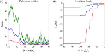Important features to observe in figure 1 are the jumps in the local-time density at the instants when the particles are incident upon the wall and reflected. These incidences occur predominantly near the release time and eventually cease (backward in time) as the particles are transported away from the wall. This escape from the wall occurs slower for smaller $\unicode[STIX]{x1D705}$ or larger $\mathit{Pr}$ , and the local times at the wall are correspondingly larger magnitude for larger $\mathit{Pr}$ .

Figure 1.

Realizations of wall-normal position (a) and local-time density process (b) for a particle released on the lower wall at $(x,z)=(3543.84\unicode[STIX]{x1D6FF}_{\unicode[STIX]{x1D708}},1891.56\unicode[STIX]{x1D6FF}_{\unicode[STIX]{x1D708}})$ for Prandtl values $\mathit{Pr}=0.1$ (green, medium), 1.0 (blue, heavy) and 10 (red, light).

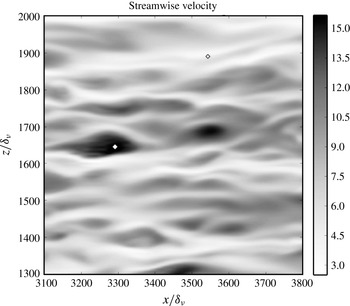
We next discuss statistics of the entire ensemble of stochastic particles for two specific release points at the wall, one point selected inside a low-speed streak and the other a high-speed streak. We are especially interested here in the role of turbulence in enhancing heat transport away from the wall, compared with pure thermal diffusion. It has sometimes between questioned whether turbulence close to the wall indeed increases thermal transport, because of the restrictions imposed on the vertical motions (e.g. Niemela & Sreenivasan Reference Niemela and Sreenivasan2003, §7.2). We thus select two points, one in a low-speed streak with mean motion toward the wall (backward in time) and the other in a high-speed streak with mean motion away from the wall (backward in time). Comparing these two points helps to identify any possible strictures on turbulent transport imposed by the solid wall. The selection is illustrated in figure 2, which plots the streamwise velocity in the buffer layer at distance $\unicode[STIX]{x0394}y=10\unicode[STIX]{x1D6FF}_{\unicode[STIX]{x1D70F}}$ above the bottom channel wall. The low-speed streaks associated with ‘ejections’ from the wall and high-speed streaks associated with ‘sweeps’ toward the wall seen there are characteristic of turbulent boundary layers (Kline et al. Reference Kline, Reynolds, Schraub and Rundstadler1967). The $x$ – $z$ coordinates of the two release points are indicated by the diamonds (♢) in figure 2 (and note that the point selected in the low-speed streak is that featured in the previous figure 1). For each of these two release points and for the three choices of Prandtl number $\mathit{Pr}=0.1$ , 1, 10, we used $N=1024$ independent solutions of equations (2.2) and (2.3) to calculate the dispersion of the stochastic trajectories and the probability density functions (PDFs) of the local-time densities backward in time. Error bars in the plots represent the standard error of the mean (s.e.m.) for the $N$ -sample averages and in addition, for the PDFs, the effects of variation in kernel density bandwidth.

Figure 2.

Streamwise velocity at normal distance $\unicode[STIX]{x0394}y=10\unicode[STIX]{x1D6FF}_{\unicode[STIX]{x1D708}}$ from the lower wall non-dimensionalized by the friction velocity $u_{\unicode[STIX]{x1D70F}}.$ The open diamonds (♢) mark the $(x,z)$ coordinates, $(3291.73\unicode[STIX]{x1D6FF}_{\unicode[STIX]{x1D708}},1644.98\unicode[STIX]{x1D6FF}_{\unicode[STIX]{x1D708}})$ and $(3543.84\unicode[STIX]{x1D6FF}_{\unicode[STIX]{x1D708}},1891.56\unicode[STIX]{x1D6FF}_{\unicode[STIX]{x1D708}}),$ of the selected release points at wall-parallel positions of high-speed (dark) and low-speed (light) streaks, respectively.

Figure 3.

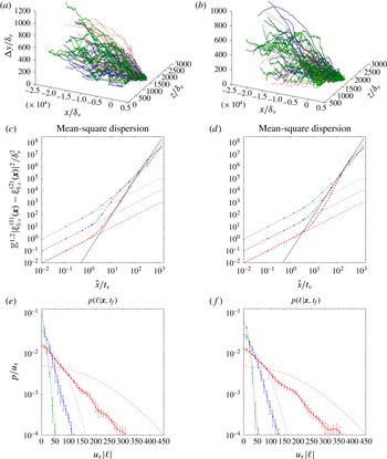
(a,c,e) Are for release at bottom wall near a high-speed streak, (b,d,f) for release near a low-speed streak. See markers on figure 2. (a,b) Show 30 representative reflected stochastic trajectories for $\mathit{Pr}=0.1$ (green, medium), 1.0 (blue, heavy) and 10 (red, light). (c,d) Plot particle dispersion (heavy) and short-time results $4\unicode[STIX]{x1D705}(3-2/\unicode[STIX]{x03C0}){\hat{s}}$ (light) for each $\mathit{Pr}$ with $\mathit{Pr}=0.1$ (green, dot, $\cdots \cdots$ ), 1.0 (blue, dash-dot, — ⋅ —) and 10 (red, dash, - - - -) and a plot (black,solid, ——) of $g(\unicode[STIX]{x1D708}/\unicode[STIX]{x1D70F}_{\unicode[STIX]{x1D708}}^{2}){\hat{s}}^{3}$ with $g=0.1$ . (e,f) Plot PDFs of (absolute values of) boundary local times for channel flow (heavy) and pure diffusion (light) for the three $\mathit{Pr}$ values with the same line styles as (c,d).

In figure 3(a,b), we show 30 representative particle trajectories for the two release points (left within a high-speed streak, right in a low-speed) and for each of the three Prandtl numbers. By eye, the ensembles of trajectories for the three different Prandtl numbers appear quite similar. In figure 3(c,d), we plot the mean-squared dispersion of the stochastic particles for the two release points and the three Prandtl numbers. There is an initial period (backward in time) where the dispersion grows with ${\hat{s}}=t_{f}-s$ as $4\unicode[STIX]{x1D705}(3-2/\unicode[STIX]{x03C0}){\hat{s}},$ which is the analytical result for a three-dimensional Brownian motion reflected from a plane (if $\tilde{W}(t)$ is standard one-dimensional Brownian motion with diffusivity $\unicode[STIX]{x1D705}$ , then $|\tilde{W}(t)|$ is the Brownian motion reflected at 0 and it is elementary to show that $\mathbb{E}^{1,2}[\{|\tilde{W}^{(1)}(t)|-|\tilde{W}^{(2)}(t)|\}^{2}]=4\unicode[STIX]{x1D705}(1-2/\unicode[STIX]{x03C0})t$ ). There is then a cross-over to a limited regime of super-ballistic separation that is close to ${\hat{s}}^{3}$ -growth. At still larger ${\hat{s}},$ the growth clearly slows but remains super-ballistic. Recall from Part I that Richardson dispersion with a cubic growth of dispersion is the physical mechanism of spontaneous stochasticity in homogeneous, isotropic turbulence. It would be quite surprising to observe Richardson dispersion in this channel-flow dataset, since the energy spectra published in Graham et al. (Reference Graham, Kanov, Yang, Lee, Malaya, Lalescu, Burns, Eyink, Szalay and Moser2016) and http://turbulence.pha.jhu.edu show that the Reynolds number is still too low to support a Kolmogorov-type inertial range. We believe that the cubic power-law growth observed arises instead from a simple combination of stochastic diffusion and mean shear, a molecular version of the turbulent shear dispersion discussed by Corrsin (Reference Corrsin1953). A toy model which illustrates this mechanism is a two-dimensional shear flow with $\boldsymbol{u}(\boldsymbol{x})=(Sy,0),$ where

Integration gives $\tilde{\unicode[STIX]{x1D709}}_{t}=\sqrt{2\unicode[STIX]{x1D705}}(S\int _{0}^{t}\tilde{W}_{y}(s)\,\text{d}s+\tilde{W}_{x}(t))$ and $\tilde{\unicode[STIX]{x1D702}}_{t}=\sqrt{2\unicode[STIX]{x1D705}}~\tilde{W}_{y}(t)$ when $(\tilde{\unicode[STIX]{x1D709}}_{0},\tilde{\unicode[STIX]{x1D702}}_{0})=(0,0),$ and the shear contributes a $t^{3}$ -term to the $x$ -component of the dispersion:

See Schütz & Bodenschatz (Reference Schütz and Bodenschatz2016) for a very similar discussion of cubic-in-time dispersion in the context of bounded shear flows and weakly turbulent Rayleigh-Bénard convection in two dimensions. In the toy model (2.15a,b ) the $y$ -component of dispersion grows only diffusively. In qualitative agreement with this simple model, we have found that the cubic power-law growth in the channel-flow particle dispersion indeed arises solely from the streamwise component of the particle separation vector. We do not show this here, but the effect can be observed in the particle trajectories plotted in figure 3(a,b), where the particles are dispersed farthest along the streamwise direction. The $t^{3}$ dispersion in (2.16) differs notably from Richardson dispersion in that it is proportional to $\unicode[STIX]{x1D705}$ and it produces no spontaneous stochasticity, since it vanishes as $\unicode[STIX]{x1D705}\rightarrow 0$ . In the channel-flow ${\hat{s}}^{3}$ -regime in figure 3(c,d) ( $10^{1}\lesssim {\hat{s}}/t_{\unicode[STIX]{x1D702}}\lesssim 10^{2}$ ) there is likewise an observable dependence on the diffusivity. These cautionary results are an admonition against interpreting any cubic or super-ballistic growth of pair separation whatsoever as evidence of spontaneous stochasticity. Richardson dispersion produces spontaneous stochasticity because of non-smooth relative advection, not simply because of super-ballistic separation.

In figure 3(e,f), we plot PDFs of the local-time density $\tilde{\ell }_{t_{f},0}(\boldsymbol{x})$ accumulated backward over the entire time interval of the channel-flow database (one flow-through time), for the two release points and the three values of Prandtl number. As could be expected, smaller $\unicode[STIX]{x1D705}$ (or larger $\mathit{Pr}$ ) correspond to more time at the wall and a PDF supported on larger local-time densities. Comparing the results for the two release points, it can be seen that particles starting on the wall inside the high-speed streak tend to spend somewhat less time near the wall than those starting near the low-speed streak. This is easy to understand, if one recalls that low-speed streaks correspond to ‘ejections’ from the wall and high-speed streaks to ‘sweeps’ toward the wall. Backward in time, however, the fluid motions are exactly reversed. Thus, particles starting at the wall inside high-speed streaks are being swept away from the wall by the fluid motion backward in time, and those starting inside low-speed streaks are brought toward the wall. However, the location of the release point has a quite small effect on the PDF of the local-time density accumulated over one flow-through time, and it is plausible that this effect would be reduced by taking $t_{f}$ even larger.

Finally, we have also plotted in figure 3(e,f) the analytical results for the local-time PDFs of a pure Brownian motion with diffusivity $\unicode[STIX]{x1D705}$ that is reflected from a planar wall (see appendix A.3 and (2.25) below). Compared with these results for Brownian motion, the corresponding channel-flow local-time PDFs exhibit in all cases a substantial reduction of time spent at the wall. These results show that turbulent fluctuations enhance transport away from the wall, even when the local flow initially carries the particles toward the wall (backward in time). Although we show these results only for two release points here, we have observed similar behaviour at all other locations on the wall that we have examined. This observation has importance for the problem of turbulent convection, where it was it was argued by Kraichnan (Reference Kraichnan1962) that ‘…the effect of the small-scale turbulence that arises locally in the shear boundary layer should be to increase heat transport’. We shall return to this issue in Part III.

2.3 Spontaneous stochasticity and anomalous dissipation

As an application of our FDR (2.13) for flows with imposed scalar fluxes at the walls, we now discuss the equivalence between spontaneous stochasticity and anomalous scalar dissipation in this context. As we shall see, the effects of the walls can be profound.

The simplest situation is the case of vanishing wall fluxes, $g\equiv 0,$ which corresponds to insulating/adiabatic walls when the scalar is the temperature and to impermeable walls when the scalar is the concentration of an advected substance (e.g. a dye, aerosol, etc.). In this case, the flux contribution proportional to the local-time density in (2.11) vanishes, and our FDR then becomes simply

This is formally identical to the relation (2.9) and (2.12) of Part I for flows in domains without boundaries, with the simple stochastic flow replaced by a reflected stochastic flow. We can therefore repeat verbatim the arguments from Part I, § 4 to conclude that, for walls that do not support fluxes, spontaneous stochasticity is equivalent to anomalous dissipation for passive scalars and for active scalars spontaneous stochasticity is (at least) necessary for anomalous scalar dissipation. For the sake of completeness, we briefly review the main ideas of this argument here. Assuming that $S\equiv 0$ for simplicity, the left-hand side of the FDR (2.17) becomes

where we have introduced the 2-time (backward-in-time) transition density

It can be shown using Young measure techniques that, at least along suitably chosen subsequences, the transition probabilities approach limiting values $p^{\ast }(\boldsymbol{y},s;\boldsymbol{y}^{\prime },s|\boldsymbol{x},t)$ , $p^{\ast }(\boldsymbol{y},s|\boldsymbol{x},t)$ as $\unicode[STIX]{x1D708},\unicode[STIX]{x1D705}\rightarrow 0$ whenever the flow domain is compact (Part I, appendix A.1). If in this limit the Lagrangian particle positions $\unicode[STIX]{x1D743}_{t,s}^{\ast }$ are deterministic, then the 2-time transition probability factorizes:

Thus, non-factorization in the limit $\unicode[STIX]{x1D708},\unicode[STIX]{x1D705}\rightarrow 0$ is the signature of spontaneous stochasticity, i.e. of the limiting particle positions $\unicode[STIX]{x1D743}_{t,s}^{\ast }$ remaining random as $\unicode[STIX]{x1D708},\unicode[STIX]{x1D705}\rightarrow 0$ . Note that the variance (2.17) can only be non-vanishing in the limit if factorization fails. Consequently, anomalous dissipation requires spontaneous stochasticity. This is true both for passive and for active scalars. In the other direction, if there is spontaneous stochasticity on a positive-measure set of $\boldsymbol{x}\in \unicode[STIX]{x1D6FA}$ , one can choose (at least for passive scalars) a suitable $\unicode[STIX]{x1D703}_{0}$ which will make the variance (2.17) positive. This implies a positive lower bound to the cumulative, volume-integrated scalar dissipation through the FDR (2.17). Thus spontaneous stochasticity and anomalous scalar dissipation are seen to be equivalent. See Part I, appendix A.2 for detailed mathematical proofs of these claims.

This result is relevant for many physical situations, such as a dye injected into a turbulent Taylor–Couette flow. The commonplace example of cream stirred into coffee is also essentially of this type, since the cup walls and surface of the stirrer are impermeable boundaries and there is also no transport of cream across the free fluid surface. The extension of our FDR (2.17) to problems with moving walls and free fluid surfaces should be relatively straightforward (and, indeed, the main result of the paper of Burdzy et al. (Reference Burdzy, Chen and Sylvester2004) was the construction of reflected Brownian processes for domains enclosed by moving boundaries). In all of these situations, any evidence for anomalous scalar dissipation is also evidence for (requires) spontaneous stochasticity.

The situations with non-vanishing fluxes through the walls are, however, essentially different. From a mathematical point of view, the problem is ‘loss of compactness’. While the trajectories of the reflected diffusion process satisfy uniformly in $\unicode[STIX]{x1D708},\unicode[STIX]{x1D705}$ the condition that $\tilde{\unicode[STIX]{x1D743}}_{t,s}^{\unicode[STIX]{x1D708},\unicode[STIX]{x1D705}}(\boldsymbol{x})\in \bar{\unicode[STIX]{x1D6FA}},$ a closed, bounded domain, the local-time densities $\tilde{\ell }_{t,s}^{\unicode[STIX]{x1D708},\unicode[STIX]{x1D705}}(\boldsymbol{x})$ may become unboundedly large as $\unicode[STIX]{x1D708},\unicode[STIX]{x1D705}\rightarrow 0.$ This creates a fundamental difficulty for arguments of the type employed previously, where limits as $\unicode[STIX]{x1D708},\unicode[STIX]{x1D705}\rightarrow 0$ were guaranteed to exist (along subsequences). To understand better the problem, consider how we might try to adapt those arguments to the present context. We can rewrite our FDR (2.13) and (2.11) as

where

and

with $\tilde{\unicode[STIX]{x1D703}}^{\unicode[STIX]{x1D708},\unicode[STIX]{x1D705}}(\boldsymbol{x},t)$ given by (2.11). If weak limits $p^{\ast }(\unicode[STIX]{x1D713}|\boldsymbol{x},t)=w\text{-}\lim _{\unicode[STIX]{x1D708},\unicode[STIX]{x1D705}\rightarrow 0}p^{\unicode[STIX]{x1D708},\unicode[STIX]{x1D705}}(\unicode[STIX]{x1D713}|\boldsymbol{x},t)$ existed, then arguments of exactly the type given before would show that anomalous dissipation requires non-factorization of $p_{2}^{\ast }$ into $p^{\ast }\cdot p^{\ast }$ and, hence, spontaneous stochasticity. The reverse argument that spontaneous stochasticity implies anomalous dissipation for passive scalars would also be essentially the same.

Simple examples show, however, that weak limits $p^{\ast }(\unicode[STIX]{x1D713}|\boldsymbol{x},t)=w$ - $\lim _{\unicode[STIX]{x1D708},\unicode[STIX]{x1D705}\rightarrow 0}p^{\unicode[STIX]{x1D708},\unicode[STIX]{x1D705}}(\unicode[STIX]{x1D713}|\boldsymbol{x},t)$ may not exist when wall fluxes are not vanishing. Consider the case where $\unicode[STIX]{x1D703}_{0}=S\equiv 0$ and the flux into the domain is a space–time constant $g(\boldsymbol{x},s)=J>0.$ In that case

and the stochastic scalar field for one realization of the Brownian process is proportional by a constant to the local-time density itself. Consider furthermore the simple case of pure heat conduction, where the advecting velocity field also vanishes, $\boldsymbol{u}^{\unicode[STIX]{x1D708}}\equiv \mathbf{0}.$ In this case, the distribution of $\tilde{\ell }_{t,0}(\boldsymbol{x})$ is known analytically in many cases. A very simple example which serves to make our point takes the domain to be the semi-infinite one-dimensional interval $\unicode[STIX]{x1D6FA}=[0,\infty )$ with boundary at 0. In that case, for $x\geqslant 0$

where $\unicode[STIX]{x1D702}(\unicode[STIX]{x1D713})$ is the Heaviside step function and

For details see appendix A.3. It is easy to see mathematically from the above expression that weak limits exist for fixed $x>0$ and, indeed,

This is also intuitively obvious, because a stochastic particle released at $x>0$ never makes it to the boundary at 0 when $\unicode[STIX]{x1D705}\rightarrow 0.$ However, the distribution $p^{\unicode[STIX]{x1D705}}(\unicode[STIX]{x1D713}|0,t)$ does not converge weakly as $\unicode[STIX]{x1D705}\rightarrow 0$ , but (2.25) implies instead that it tends to become uniformly spread on the semi-infinite interval. This also makes sense, because a particle released at 0 should tend to stay there as $\unicode[STIX]{x1D705}\rightarrow 0$ and the local-time density at 0 will diverge (in fact, if we consider the 1-point compactification $[0,\infty ]$ of the range $[0,\infty )$ of possible scalar values, then $\lim _{\unicode[STIX]{x1D705}\rightarrow 0}p^{\unicode[STIX]{x1D705}}(\unicode[STIX]{x1D713}|0,t)=\unicode[STIX]{x1D6FF}_{\infty }(\unicode[STIX]{x1D713}),$ the delta function at infinity. However, this compactification of the problem does not yield any result on spontaneous stochasticity).

The physical origin of the divergence in this simple example is a scalar boundary layer near $x=0.$ A direct solution of the Neumann problem for the scalar field or integration over the above distribution shows that

for a suitable scaling function $f$ . See appendix A.1. There is thus a scalar boundary layer of thickness ${\sim}\sqrt{\unicode[STIX]{x1D705}t}$ near 0 where the scalar field diverges as $\unicode[STIX]{x1D703}\sim J\sqrt{t/\unicode[STIX]{x1D705}}$ as $\unicode[STIX]{x1D705}\rightarrow 0$ . Because there is a constant flux $J$ into the domain and diffusive transport into the interior vanishes as $\unicode[STIX]{x1D705}\rightarrow 0$ , there is a ‘pile up’ of the scalar near $x=0$ . The scalar dissipation field due to this boundary layer is

from which one can infer a total scalar dissipation $\propto J^{2}\sqrt{t/\unicode[STIX]{x1D705}}\rightarrow \infty$ as $\unicode[STIX]{x1D705}\rightarrow 0$ . This ‘dissipative anomaly’ occurs even though there is clearly no spontaneous stochasticity in this simple example with $\boldsymbol{u}^{\unicode[STIX]{x1D708}}\equiv 0!$

The above example shows that the ‘loss of compactness’ is not a mere technical mathematical difficulty, but instead that there may no longer be equivalence of spontaneous stochasticity and non-vanishing dissipation. Scalar boundary layers in wall-bounded flow domains with flux through the walls are a new possible source of scalar dissipation that can be non-zero (or even diverging) as $\unicode[STIX]{x1D708},\unicode[STIX]{x1D705}\rightarrow 0$ , quite distinct from the spontaneous stochasticity mechanism. Another perhaps more elementary way to see the problem posed by wall fluxes is to exploit formula (2.6) for the boundary local time to write

where $p_{2}^{\unicode[STIX]{x1D708},\unicode[STIX]{x1D705}}(\boldsymbol{y},s;\boldsymbol{y}^{\prime },s^{\prime }|\boldsymbol{x},t)$ for $s,s^{\prime }<t$ is the 2-time transition probability density function with respect to the Lebesgue measure, defined in (2.19). On the face of it, this appears to be quite similar to the analogous formulae for the scalar variance associated with the initial data or internal sources, e.g. (2.18). However, in the variance associated with $\unicode[STIX]{x1D703}_{0}$ or $S,$ the transition probability densities appear only in the combinations $\text{d}^{d}y~\text{d}^{d}y^{\prime }~p_{2}^{\unicode[STIX]{x1D708},\unicode[STIX]{x1D705}}(\boldsymbol{y},s;\boldsymbol{y}^{\prime },s^{\prime }|\boldsymbol{x},t)$ and $\text{d}^{d}y~p^{\unicode[STIX]{x1D708},\unicode[STIX]{x1D705}}(\boldsymbol{y},s|\boldsymbol{x},t),$ and thus only involve the probability measures themselves and not their densities. Compactness arguments suffice to show that limits of the probability measures and associated integrals exist (along subsequences) as $\unicode[STIX]{x1D708},\unicode[STIX]{x1D705}\rightarrow 0.$ On the other hand, the formula (2.30) involves the probability density function evaluated on the boundary of the domain. Even if the (weak) limit of the particle probability measures have density functions $p_{2}^{\ast }(\boldsymbol{y},s;\boldsymbol{y}^{\prime },s^{\prime }|\boldsymbol{x},t)$ and $p^{\ast }(\boldsymbol{y},s|\boldsymbol{x},t),$ they are undefined at the boundary $\unicode[STIX]{x2202}\unicode[STIX]{x1D6FA}$ , which is a Lebesgue zero-measure set. In general, the probability density functions will not have pointwise limits as $\unicode[STIX]{x1D708},\unicode[STIX]{x1D705}\rightarrow 0$ and, in the example of pure diffusion on the half-line discussed above, they diverge when all three points $\boldsymbol{x},$ $\boldsymbol{y}$ , $\boldsymbol{y}^{\prime }$ are located on the left boundary at 0!

On the other hand, we can extend all of our results relating spontaneous stochasticity and anomalous scalar dissipation to general choices of wall fluxes, if we make the additional assumption that pointwise limits of densities exist for all $\boldsymbol{x},\boldsymbol{y},\boldsymbol{y}^{\prime }\in \unicode[STIX]{x1D6FA}$

so that the limit of the variance in (2.30) exists and is given by the formula

This assumption, of course, rules out the presence of scalar boundary layers of the type discussed above. The necessity of spontaneous stochasticity for anomalous scalar dissipation is immediate, because factorization $p_{2}^{\ast }(\boldsymbol{y},s;\boldsymbol{y}^{\prime },s^{\prime }|\boldsymbol{x},t)=p^{\ast }(\boldsymbol{y},s|\boldsymbol{x},t)p^{\ast }(\boldsymbol{y}^{\prime },s^{\prime }|\boldsymbol{x},t)$ of the limit densities implies that all variances tend to zero. If the scalar is passive, then sufficiency holds as well. Consider, for simplicity, the case of vanishing internal source $S\equiv 0.$ As in Part I, § 4 and appendix A, we can make a smooth choice of scalar initial data $\unicode[STIX]{x1D703}_{0}$ so that the volume average of the limiting variance in (2.18) is strictly positive, whenever non-factorization holds for a positive-measure set of $\boldsymbol{x}\in \unicode[STIX]{x1D6FA}$ . The limit variance in (2.32) involving the boundary flux $g$ is non-negative when it exists at all. If the covariance term involving both $\unicode[STIX]{x1D703}_{0}$ and $g$ is negative, then by taking $\unicode[STIX]{x1D703}_{0}\rightarrow -\unicode[STIX]{x1D703}_{0}$ the covariance can be made positive without changing the sign of either of the two variances involving $\unicode[STIX]{x1D703}_{0}$ and $g$ separately. In this manner, for any possible choice of wall fluxes $g,$ an initial condition $\unicode[STIX]{x1D703}_{0}$ for the passive scalar advection equation always exists so that scalar dissipation is non-vanishing as $\unicode[STIX]{x1D708},\unicode[STIX]{x1D705}\rightarrow 0.$ The same conclusion holds also for an active scalar, barring a ‘conspiracy’ in which all Lagrangian particles at time $0$ originating from almost every point $\boldsymbol{x}\in \unicode[STIX]{x1D6FA}$ at time $t$ are confined to a single isoscalar surface of $\unicode[STIX]{x1D703}_{0}$ for that $\boldsymbol{x},$ even when varying over all possible $\unicode[STIX]{x1D703}_{0}.$ It is this unlikely coincidence which must be ruled out by a rigorous proof. In this manner we see that all of our previous conclusions for flows without walls or for zero fluxes at the walls, can be extended to the case of general wall-fluxes $g,$ whenever the stringent assumption (2.31) on pointwise limits is valid.

3.1 Stochastic representation and fluctuation–dissipation relation

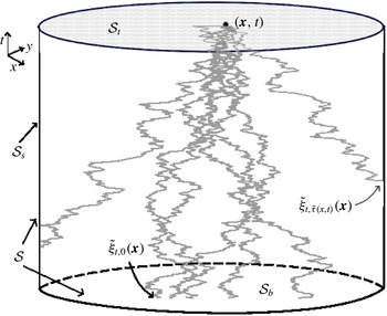
The standard stochastic representation of solutions of the problem (3.1) involves stochastic particles which are stopped at the boundary, contributing a term due to the value maintained at the wall (Keanini Reference Keanini2007; Soner Reference Soner2007; Oksendal Reference Oksendal2013). The stochastic flow may again be defined with reflection at the boundary, governed by the equation (2.2) involving the boundary local time. The new notion is the boundary (first) hitting time or stopping time, which is defined for $\boldsymbol{x}\in \unicode[STIX]{x1D6FA}$ by the larger of $\sup \{s:\tilde{\unicode[STIX]{x1D743}}_{t,s}(\boldsymbol{x})\in \unicode[STIX]{x2202}\unicode[STIX]{x1D6FA}\}$ , the first time going in reverse to hit the spatial boundary, and the initial time 0, or

This is the first time (going backward) at which the stochastic Lagrangian particle hits the space–time exit surface ${\mathcal{S}},$ the union of the ‘side surface’ ${\mathcal{S}}_{s}=\unicode[STIX]{x2202}\unicode[STIX]{x1D6FA}\times [0,t)$ and the ‘base’ ${\mathcal{S}}_{b}=\unicode[STIX]{x1D6FA}\times \{0\}$ of the right cylindrical domain ${\mathcal{D}}=\unicode[STIX]{x1D6FA}\times [0,t)$ in $(d+1)$ -dimensional space–time, when starting at a point $(\boldsymbol{x},t)$ in the ‘top’ ${\mathcal{S}}_{t}=\unicode[STIX]{x1D6FA}\times \{t\}.$ See figure 4.

Figure 4.

A schematic of the space–time domain ${\mathcal{D}}$ for a disk-shaped space domain $\unicode[STIX]{x1D6FA}\subseteq \mathbb{R}^{2}$ , together with realizations of the process $\tilde{\unicode[STIX]{x1D743}}_{t,s}(\boldsymbol{x})$ satisfying (2.2) and stopped at the exit surface ${\mathcal{S}}={\mathcal{S}}_{b}\cup {\mathcal{S}}_{s}$ . Some trajectories reach the base ${\mathcal{S}}_{b}$ at random points $\tilde{\unicode[STIX]{x1D743}}_{t,0}(\boldsymbol{x})$ whereas others hit the side surface ${\mathcal{S}}_{s}$ at points $\tilde{\unicode[STIX]{x1D743}}_{t,\tilde{\unicode[STIX]{x1D70F}}(\boldsymbol{x},t)}(\boldsymbol{x})$ and are stopped there.

To state conveniently the stochastic representation, we define the function which gives the data on ${\mathcal{S}}$ :

Using the backward It $\bar{\text{o}}$ formula (2.7) and integrating from time $t$ down to the hitting time $\tilde{\unicode[STIX]{x1D70F}}(\boldsymbol{x},t)$ gives

where we used the fact that $\tilde{\ell }_{t,s}(\boldsymbol{x})\equiv 0$ for all $\tilde{\unicode[STIX]{x1D70F}}(\boldsymbol{x},t)<s<t$ and also used the system (3.1). Taking the expectation over the Brownian motion then yields for solutions of the initial boundary-value problem the following stochastic representation:

See Keanini (Reference Keanini2007), Soner (Reference Soner2007) and Oksendal (Reference Oksendal2013) for more details. In particular, the It $\bar{\text{o}}$ integral in (3.4) is a (backward) martingale by the optional stopping theorem (Oksendal Reference Oksendal2013). This formula represents the solution $\unicode[STIX]{x1D703}(\boldsymbol{x},t)$ to the scalar advection–diffusion equation as an average over randomly sampled sources and initial boundary data.

It is now straightforward to obtain our first version of a fluctuation–dissipation relation by mimicking previous arguments. Applying the It $\bar{\text{o}}$ isometry valid with the random stopping time as the lower range of the integral (see e.g. Oksendal Reference Oksendal2013, Theorem 7.4.1)

Thus we obtain from (3.4), (3.5) that

Finally, averaging over the space domain yields

This exact result is one possible version of a fluctuation–dissipation relation for scalar turbulence with general Dirichlet boundary conditions.

Unlike our previous relations, however, the right-hand side of (3.8) above is not the total time-integrated scalar dissipation over the entire domain of the flow. The relation easily yields a lower bound on the total scalar dissipation by simply extending the time integration down to $s=0$ ,

because the $s$ -integrand is non-negative and the reflected stochastic flow is volume preserving, so that the Jacobian of the change of variables from $\tilde{\unicode[STIX]{x1D743}}_{t,s}(\boldsymbol{x})$ to $\boldsymbol{x}$ is unity. The difference between the right-hand and left-hand sides is

where

is the set of positions $\boldsymbol{x}$ for which the stochastic particle has already hit the boundary by time $s$ (going backward). The inequality (3.9) thus fails to be an equality because of the missing contributions to total dissipation at positions of reflected particles. We shall discuss further below the sharpness of the inequality (3.9) and whether it should, in a suitable limit, become equality.

3.2 Numerical results

To gain further insight, we present now some numerical results on PDFs of hitting times for the channel-flow database. We considered two release points in the buffer layer at height $\unicode[STIX]{x0394}y=10\unicode[STIX]{x1D6FF}_{\unicode[STIX]{x1D70F}}$ above the bottom wall and at the final time $t_{f}$ of the database. The wall-parallel positions of the release points are those shown in figure 2, and thus one is in a high-speed streak and the other in a low-speed streak. It turns out that to calculate hitting-time PDFs accurately using $N$ -sample ensembles of particles is quite difficult, because most particles take a very long time to first hit the boundary. For our results presented here, we evolved $N=14\,336$ samples of stochastic particles solving (2.2) for three Prandtl numbers $\mathit{Pr}=0.1$ , 1, 10 at both release points. Note that hitting times $\unicode[STIX]{x1D70F}$ satisfying $t_{f}-\unicode[STIX]{x1D70F}\ll \unicode[STIX]{x1D70F}_{\unicode[STIX]{x1D708}}$ and $t_{f}-\unicode[STIX]{x1D70F}\gg \unicode[STIX]{x1D70F}_{\unicode[STIX]{x1D708}}$ are both very rare events which could not be observed even with so many samples. We thus consider here the logarithmic variable $\unicode[STIX]{x1D706}\equiv \ln ((t_{f}-\unicode[STIX]{x1D70F})/\unicode[STIX]{x1D70F}_{\unicode[STIX]{x1D708}})$ which is appropriate to typical values and calculate PDFs $p(\unicode[STIX]{x1D706}|\boldsymbol{x},t_{f})$ . The numerical procedures are discussed at length in appendix D.2. Here we just note that the PDFs are obtained up to the largest available $\unicode[STIX]{x1D706}=\ln (t_{f}/\unicode[STIX]{x1D70F}_{\unicode[STIX]{x1D708}})\doteq 7.17$ and down to $\unicode[STIX]{x1D706}=-1,$ but the PDFs at the two extremes contain further errors that are not indicated by the error bars (representing both s.e.m. for $N$ -samples averages and variation with kernel bandwidth). The PDFs for $\unicode[STIX]{x1D706}<1.6$ are shifted to the right by approximately 5 %, because our time step $\unicode[STIX]{x0394}s\doteq 2\times 10^{-3}$ cannot fully resolve the smaller hitting times. For $\unicode[STIX]{x1D706}>6.5$ the PDFs from kernel density estimates are too small, because of the end point effect due to unavailability of samples for $\unicode[STIX]{x1D706}>7.17.$ Our numerical procedures show the same deficiencies when applied to pure Brownian motion, but successfully recover the known analytical results for that case in the range $1.6<\unicode[STIX]{x1D706}<6.5$ .

Figure 5.

PDFs of the logarithmic hitting-time variable $\unicode[STIX]{x1D706}=\ln ((t_{f}-\unicode[STIX]{x1D70F})/\unicode[STIX]{x1D70F}_{\unicode[STIX]{x1D708}})$ . (a) Particles released in a high-speed streak, (b) particles released in a low-speed streak, for channel flow (heavy) and pure diffusion (light) for Prandtl numbers $\mathit{Pr}=0.1$ (green, dot, $\cdots \cdots$ ), 1.0 (blue, dash-dot, — ⋅ —) and 10 (red, dash, - - - -).

We plot in figure 5 the PDFs $p(\unicode[STIX]{x1D706}|\boldsymbol{x},t_{f})$ for the two choices of $\boldsymbol{x},$ the left panel corresponding to particles released in a high-speed streak and the right to particles released in a low-speed streak. We also plot for comparison the analytical results for hitting-time PDFs with pure diffusion (see (D 4) of appendix D.2). One can see in figure 5 a very strong effect of the release point on the hitting-time statistics, unlike the situation for the boundary local times accumulated over one flow-through time. At $\mathit{Pr}=0.1$ and 1, hitting times are clearly larger than those of pure diffusion for release in a high-speed streak and smaller for release in a low-speed streak. This effect is easy to understand, because particles released in a low-speed streak are advected toward the wall backward in time, and those released in a high-speed streak swept away from the wall. This effect is not observed for $\mathit{Pr}=10$ , with hitting times for pure diffusion very obviously shorter than those for advected particles started in both high-speed and low-speed streaks. This occurs presumably because advection alone can never bring a particle to the wall in a finite time (because of the vanishing velocity there) and as diffusivity $\unicode[STIX]{x1D705}$ decreases one sees more strongly the effect of fluid advection, which transports the particles away from the wall. One can see in general a strong effect of diffusivity on the hitting times, with smaller values of $\unicode[STIX]{x1D705}$ (or larger $\mathit{Pr}$ ) leading to larger hitting times backward in time. We shall refer to this property in our discussion below of the sharpness of the inequality (3.9). However, we first exploit this inequality to prove also for Dirichlet boundary conditions that spontaneous stochasticity is sufficient for anomalous dissipation of passive scalars.

3.3 Spontaneous stochasticity implies anomalous dissipation

The argument is very similar to those given earlier. To present it first in the simplest context, we consider a decaying scalar with vanishing source ( $S=0$ ). We first introduce an analogue of the formula (2.18) for the variance which constitutes the lower bound. There is a natural measure on the exit surface ${\mathcal{S}}$ (see figure 4) which is just the $d$ -dimensional Hausdorff measure $H^{d}$ on subsets of $(d+1)$ -dimensional space–time, restricted to ${\mathcal{S}}.$ This can be described in elementary terms using natural $d$ -dimensional coordinates $\unicode[STIX]{x1D748}$ on ${\mathcal{S}},$ where on ${\mathcal{S}}_{b}$ we have $\unicode[STIX]{x1D748}=(\boldsymbol{y},0)$ for $\boldsymbol{y}\in \unicode[STIX]{x1D6FA}$ and on ${\mathcal{S}}_{s}$ we have $\unicode[STIX]{x1D748}=(\boldsymbol{z},\unicode[STIX]{x1D70F})$ for $\boldsymbol{z}\in \unicode[STIX]{x2202}\unicode[STIX]{x1D6FA},$ the presumed smooth bounding wall surface, and $\unicode[STIX]{x1D70F}\in [0,t].$ Then for $\unicode[STIX]{x1D748}\in {\mathcal{S}}$

Here $H^{d-1}$ is the $(d-1)$ -dimensional Hausdorff measure on the smooth wall surface $\unicode[STIX]{x2202}\unicode[STIX]{x1D6FA}$ (that is, the usual $(d-1)$ -dimensional surface area $\text{d}S$ ). We can then also define the delta distribution $\unicode[STIX]{x1D6FF}_{{\mathcal{S}}}(\unicode[STIX]{x1D748}^{\prime },\unicode[STIX]{x1D748})$ on ${\mathcal{S}}$ with respect to measure $H^{d},$ so that

for all smooth functions on ${\mathcal{S}},$ and we can likewise decompose this delta function as

Denoting by $\tilde{\unicode[STIX]{x1D748}}(\boldsymbol{x},t)=(\tilde{\unicode[STIX]{x1D743}}_{t,\tilde{\unicode[STIX]{x1D70F}}(\boldsymbol{x},t)}(\boldsymbol{x}),\tilde{\unicode[STIX]{x1D70F}}(\boldsymbol{x},t))$ the space–time point where the trajectory first hits ${\mathcal{S}}$ (going backward in time), we can then introduce 1-time transition probability densities for a particle to go backward in time from points $(\boldsymbol{x},t)$ on the ‘top’ surface $\unicode[STIX]{x1D6FA}\times \{t\}$ of the space–time cylinder and to arrive first to ${\mathcal{S}}$ at the point $\unicode[STIX]{x1D748}\in {\mathcal{S}}$ :

This probability density is normalized with respect to $H^{d}$ on ${\mathcal{S}}$ so that

In these terms we obtain a simple formula for the stochastic representation (3.5) in the case of vanishing scalar source:

We note in passing here that there is another representation for $q(\unicode[STIX]{x1D748}|\boldsymbol{x},t)$ in terms of a process of stochastic Lagrangian particles which is distinct from that considered so far. Rather than letting the particles reflect off the wall, one can instead kill the particles when they hit the wall (absorbing boundary conditions). If $k(\boldsymbol{a},s|\boldsymbol{x},t)$ for $s<t$ is the transition probability density for this killed process backward in time, then

Here we make use of the general connection between the joint density function of the hitting time and location and between the normal derivative of the transition probability for the killed process; see Freĭdlin (Reference Freĭdlin1985) and Hsu (Reference Hsu1986). This alternative stochastic interpretation will prove useful for calculations in appendix B.

We can obtain a similar formula as (3.17) for the variance, if we introduce also the corresponding twofold transition probabilities

so that

These results are formally identical to those for the sourceless $(S=0)$ scalar in domains without boundary or with zero-flux Neumann conditions at the wall. Furthermore, ${\mathcal{S}}$ is a compact subset of space–time. Thus, we can exactly mimic our previous arguments with no change. Limits $q^{\ast },q_{2}^{\ast }$ as $\unicode[STIX]{x1D708}_{j},\unicode[STIX]{x1D705}_{j}\rightarrow 0$ always exist along suitable subsequences $\unicode[STIX]{x1D708}_{j},\unicode[STIX]{x1D705}_{j}$ . If the limits were deterministic, then one would have

so that $q_{2}^{\ast }$ would factorize in a product of two $q^{\ast }$ values. However, if the limits are non-deterministic so that $q_{2}^{\ast }$ does not factorize for a positive-measure set of $\boldsymbol{x}$ at time $t$ , then there must be some smooth choice of $\unicode[STIX]{x1D6E9}=(\unicode[STIX]{x1D703}_{0},\unicode[STIX]{x1D713})$ that makes the non-negative space-averaged variance in (3.20) in fact non-zero. For such choice of initial condition $\unicode[STIX]{x1D703}_{0}$ and boundary conditions $\unicode[STIX]{x1D713}$ , the space-averaged and time-integrated scalar dissipation will then be non-zero taking the limit $\unicode[STIX]{x1D708}_{j},\unicode[STIX]{x1D705}_{j}\rightarrow 0.$ As before, this argument works rigorously only for a passive scalar, not an active one. An additional limitation discussed further in appendix C is that we cannot use this argument to prove, for a fixed choice of the boundary data $\unicode[STIX]{x1D713},$ that spontaneous stochasticity implies there exists a smooth initial datum $\unicode[STIX]{x1D703}_{0}$ for which the scalar dissipation rate is positive (These comments have implications for the problem of Rayleigh–Bénard convection with fixed temperatures at top/bottom plates, which is discussed in Part III. There is some evidence for Richardson dispersion of Lagrangian particles in numerical simulations of turbulent convection (Schumacher Reference Schumacher2008). However, even if there were compelling evidence for spontaneous stochasticity associated with this effect, we could not rigorously conclude from our results that there is anomalous thermal dissipation. First, the temperature is an active scalar in that case and, second, our present arguments do not work with fixed boundary data). Minor changes to these arguments are needed to incorporate a bulk source $S$ and we leave details also to appendix C.

The previous arguments do not imply that spontaneous stochasticity is required for anomalous scalar dissipation with imposed scalar values at the wall. Even if the factorization (3.21) holds and there is no spontaneous stochasticity, the variance in (3.20) provides only a lower bound to the scalar dissipation. Hence, the scalar dissipation rate can tend to a non-zero limit even when the variance vanishes! This is not just a failure of the proof, but also an indication that other physical mechanisms are available to produce anomalous dissipation with Dirichlet boundary conditions. The most obvious alternative mechanism is a narrow scalar boundary layer at the walls. One can imagine a flow with extremely rapid advective mixing in the interior and with opposite scalar values $\pm \unicode[STIX]{x1D713}_{0}$ imposed at two ends, so that large scalar gradients of the order $\unicode[STIX]{x1D735}\unicode[STIX]{x1D703}\sim O(\unicode[STIX]{x1D713}_{0}/\unicode[STIX]{x1D705})$ are achieved in a boundary layer of thickness ${\sim}O(\unicode[STIX]{x1D705})$ and a near-zero scalar amplitude $\unicode[STIX]{x1D703}\simeq 0$ occurs over the bulk of the domain. Such a flow would be the simplest that provides anomalous scalar dissipation from a scalar boundary-layer mechanism. For example, one might consider a fluid undergoing solid-body rotation with frequency $\unicode[STIX]{x1D714}$ in the interior of the domain and an imposed inhomogeneous temperature distribution on the boundary varying between $-\unicode[STIX]{x1D713}_{0}$ and $+\unicode[STIX]{x1D713}_{0}.$ In the rotating frame of reference, this would correspond to a motionless fluid (pure heat conduction) but with a time-dependent boundary temperature oscillating with frequency $\unicode[STIX]{x1D714}$ between the extreme values $\pm \unicode[STIX]{x1D713}_{0}$ .

As the simplest example of this type, consider pure diffusion on the interval $[0,H]$ with $\unicode[STIX]{x1D703}_{0}=S\equiv 0$ and boundary temperatures specified as $\unicode[STIX]{x1D713}(0,t)=\unicode[STIX]{x1D713}_{0}\sin (\unicode[STIX]{x1D714}t)$ and $\unicode[STIX]{x1D713}(H,t)=0.$ In this case, the stochastic scalar field is simply

The scalar field $\unicode[STIX]{x1D703}(x,t)=\mathbb{E}[\tilde{\unicode[STIX]{x1D703}}(\boldsymbol{x},t)]$ can be constructed with the knowledge of the hitting-time distribution at zero for Brownian motion on the half-line, which is

See appendix B. The solution $\unicode[STIX]{x1D703}(x,t)$ of the conduction problem can be obtained by integration over the above distribution, and scalar gradients can then be explicitly computed; see (B 23). Temperature fluctuations are found to propagate with velocity $(\unicode[STIX]{x1D705}\unicode[STIX]{x1D714})^{1/2}$ and travel to distances $(\unicode[STIX]{x1D705}/\unicode[STIX]{x1D714})^{1/2}$ away from the wall. In this small boundary-layer region, the scalar field gradients diverge as $\unicode[STIX]{x2202}_{x}\unicode[STIX]{x1D703}\sim \unicode[STIX]{x1D713}_{0}(\unicode[STIX]{x1D714}/\unicode[STIX]{x1D705})^{1/2}$ as $\unicode[STIX]{x1D705}\rightarrow 0.$ We obtain

See (B 14) for a more precise statement. The scalar field in this simple example exhibits anomalous dissipation if $\unicode[STIX]{x1D714}$ is very large for $\unicode[STIX]{x1D705}\rightarrow 0,$ e.g. with $\unicode[STIX]{x1D714}\sim \unicode[STIX]{x1D705}^{-\unicode[STIX]{x1D6FC}}$ for $\unicode[STIX]{x1D6FC}\geqslant 1$ . In particular, for $\unicode[STIX]{x1D6FC}=1$ the limiting scalar dissipation rate is non-zero and finite as $\unicode[STIX]{x1D705}\rightarrow 0,$ with scalar gradients and boundary-layer thicknesses as suggested in the previous paragraph. Thus, just as for flux boundary conditions, thin scalar boundary layers can be a source of non-zero (possibly diverging) dissipation as $\unicode[STIX]{x1D708},\unicode[STIX]{x1D705}\rightarrow 0$ .

3.4 Equality fluctuation–dissipation relation

We now return to the question whether our lower bound (3.9) on the cumulative (time- and space-integrated) scalar dissipation may in fact be an equality. This is certainly not true in the $t\rightarrow \infty$ limit with $\unicode[STIX]{x1D705},\unicode[STIX]{x1D708}$ fixed. We note that

since the boundary hitting times are finite almost surely for $\unicode[STIX]{x1D705},\unicode[STIX]{x1D708}>0$ (see Karlin & Taylor Reference Karlin and Taylor1981, chap. 15, § 11) and, thus, the particle released in the far distant future $t$ will certainly hit the space boundary $\unicode[STIX]{x2202}\unicode[STIX]{x1D6FA}$ before $s$ (moving backward in time). Thence by dominated convergence

and the contribution of reflected particles coincides at long times with the total dissipation. A strengthened conclusion is that

for some function $\unicode[STIX]{x1D6FF}(t)\geqslant 0$ such that $\lim _{t\rightarrow \infty }\unicode[STIX]{x1D6FF}(t)=\infty ,\lim _{t\rightarrow \infty }\unicode[STIX]{x1D6FF}(t)/t=0$ . This is true because the difference $t-s\geqslant \unicode[STIX]{x1D6FF}(t)$ for all such $s$ . In that case, however, we see that

where $\unicode[STIX]{x1D6E5}^{\unicode[STIX]{x1D708},\unicode[STIX]{x1D705}}(t)$ is the difference in (3.10). Thus, our lower bound (3.9) on space–time average dissipation becomes vacuous as $t\rightarrow \infty$ , with the long-time limit of the lower bound simply tending to zero as reflected particles fill the entire domain.

Now consider the opposite limit with $\unicode[STIX]{x1D708},\unicode[STIX]{x1D705}\rightarrow 0$ for fixed $t$ . If we keep $\unicode[STIX]{x1D708}$ fixed so that the velocity stays smooth, then no particles will reach the boundary in the finite time interval $[0,t]$ as $\unicode[STIX]{x1D705}\rightarrow 0$ . An increase of hitting times with decreasing $\unicode[STIX]{x1D705}$ for fixed $\unicode[STIX]{x1D708}$ is clearly observed in figure 5. In this limit, the inequality in our lower bound becomes equality. However, as long as $\boldsymbol{u}$ is smooth, then there will be no dissipative anomaly and the scalar dissipation will vanish! Thus, this limit is of little interest. On the other hand, if we take $\unicode[STIX]{x1D708},\unicode[STIX]{x1D705}\rightarrow 0$ together, then it is possible that the particles will hit the boundary and reflect. In fact, this must be the case if there is a scalar dissipative anomaly at finite times $t$ for flux boundary conditions and vanishing initial data of the scalar and vanishing scalar sources, since then the FDR (2.13) is solely due to the contribution of the boundary local times in (2.11). If particles continue to hit the boundary as $\unicode[STIX]{x1D708},\unicode[STIX]{x1D705}\rightarrow 0$ for fixed time $t,$ then our lower bound must be a strict inequality (but possibly non-vanishing for finite $t$ ).

It is straightforward, however, to obtain an equality relation for the scalar dissipation by using the same derivation as for flux boundary conditions, namely, by using the backwards It $\bar{\text{o}}$ formula (2.7) and integrating from time $t$ down to 0, rather than stopping when hitting the boundary. This argument yields for the scalar itself

and for the variance

which is our second version of a fluctuation–dissipation relation for Dirichlet boundary conditions of the scalar. The total scalar dissipation is now obtained, with the contribution of the reflected particles represented by the boundary local-time density term on the left. Unfortunately, this new formula is not very convenient for mathematical analysis, because the scalar boundary flux $g(\boldsymbol{x},t)=-\unicode[STIX]{x1D741}\boldsymbol{\cdot }\unicode[STIX]{x1D735}\unicode[STIX]{x1D703}(\boldsymbol{x},t)$ is no longer a known input, but is instead a space–time fluctuating quantity which must be determined from the solution of the scalar advection–diffusion equation. This relation thus has a mixed Euler–Lagrangian character, because it involves both the Eulerian scalar field $\unicode[STIX]{x1D703}(\boldsymbol{x},t)$ and the stochastic Lagrangian flow $\tilde{\unicode[STIX]{x1D743}}_{t,s}.$ Despite being clumsy for mathematical use, this relation is the physically most natural version of the FDR for scalar Dirichlet boundary conditions, and provides insight into the Lagrangian origin of scalar dissipation. In appendix B.2, we explicitly demonstrate the equivalence of the formula (3.29) to the more standard representation (3.17) for the simple example of heat conduction with oscillating wall temperature.

3.5 Mixed boundary conditions

The extension of the previous results to scalars with general mixed Dirichlet–Neumann conditions (1.2), (1.3) is straightforward. Again, one considers the backward stochastic flow with reflection at the boundary. To derive an FDR in the form of an inequality like (3.8), one must stop those particles which hit $\unicode[STIX]{x2202}\unicode[STIX]{x1D6FA}_{D}$ before time 0 (going backward). The particles which hit $\unicode[STIX]{x2202}\unicode[STIX]{x1D6FA}_{N}$ are simply reflected. Results like (3.7) and (3.8) are obtained, except that now the stopping time $\tilde{\unicode[STIX]{x1D70F}}(\boldsymbol{x},t)$ is the first time to hit $\unicode[STIX]{x2202}\unicode[STIX]{x1D6FA}_{D}$ (or 0, whichever is larger) and the variance on the left includes contributions from the local-time density at the piece $\unicode[STIX]{x2202}\unicode[STIX]{x1D6FA}_{N}$ of the boundary. This FDR inequality omits the contribution to scalar dissipation at locations of particles reflected from  $\unicode[STIX]{x2202}\unicode[STIX]{x1D6FA}_{D}$ . It is also easy to obtain an FDR equality like (3.30) by stopping no particles. It has an identical form to (3.30) and the sole difference is that $g(\boldsymbol{x},t)=-\unicode[STIX]{x1D741}\boldsymbol{\cdot }\unicode[STIX]{x1D735}\unicode[STIX]{x1D703}(\boldsymbol{x},t)$ is a specified function for points $\boldsymbol{x}\in \unicode[STIX]{x2202}\unicode[STIX]{x1D6FA}_{N}$ but must be obtained for $\boldsymbol{x}\in \unicode[STIX]{x2202}\unicode[STIX]{x1D6FA}_{D}$ by solving the advection–diffusion equation. We shall make use of this version of the FDR in our discussion of turbulent Rayleigh–Bénard convection in the following Part III.