II. Literature on Gender-Specific Wine-Tasting Results

Little has been published about the potential differences between women's and men's relative preferences for the same wines.

The findings of those who have evaluated gender-related differences in taste preference are summarized in the Introduction above. In particular, Corbin (Reference Corbin2006) undertakes a literature review and finds more than forty articles on the topic, but her findings do not uncover even one study concerning wine. The literature review in Bodington (Reference Bodington2015b), regarding applications of rank preference and mixture models to taste tests, does not uncover any reports concerning wine. Further, with the exception of Critchlow (Reference Critchlow1985), who finds that mothers and sons have different preferences for crackers, none of the studies reviewed in Bodington (Reference Bodington2015b) report any gender-related differences at all.

A search of the Journal of Wine Economics, Journal of Wine Research, American Journal of Enology and Viticulture, Chemical Senses, and Psychological Science does not yield a comparison of gender-related wine preferences. Hanni and Utermohlen (Reference Hanni and Utermohlen2010, 8) have self-published an evaluation of 1,485 responses to an online survey of wine consumers and found that people “who like sweeter wines are more likely to be female and younger,” while people who like big red wines tend to be male and older. That report and many other articles about women's and men's preferences in the popular wine press (e.g., Jancis Robinson's Purple Pages website, the Wall Street Journal, Wine Business, and Wine Spectator) are not summarized here, because they do not describe a blind-tasting protocol, nor do they disclose gender- and taster-specific data.

In fairness to the authors of wine-related articles in the publications noted above, they seek to answer specific non-gender-related questions, and they do not purport to have any conclusions about differences between women and men in wine-tasting results. Subject to that qualification, the literature to date does not appear to contain a formal analysis of whether women and men assign the same scores to the same wines, giving consideration to idiosyncratic preferences and randomness.

III. Scores for Women and Men in Twenty-Three Tastings

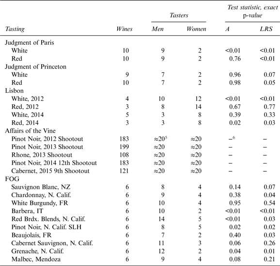
Scores have been obtained for female and male tasters for two flights of wines in the 1976 Judgment of Paris (Paris), two flights in the 2012 Judgment of Princeton (Princeton), for more than one hundred fifty wines in each of five tastings sponsored by the California-based Affairs of the Vine (Affairs), for four panels of University of Lisbon students using the Mundus Vini tasting form developed by the German publisher Meininger Verlag (Lisbon), and for one flight during each of ten tastings organized by the San Francisco–based wine-tasting group FOG (FOG). All tasting data have been uploaded to the Journal of Wine Economics data site, and the tastings are summarized in Table 1.

Table 1

Summary of Wines, Tasters, and Tests of Apparent Randomness

Note: SLH, Santa Lucia Highlands.

Scores assigned by individual tasters in Paris are from Hulkower (Reference Hulkower2009, Tables 3 and 8), in Princeton from Ashenfelter and Storchmann (Reference Ashenfelter and Storchmann2012, Tables 3 and 4), for Affairs from its website affairsofthevine.com,Footnote ¹ for Lisbon from Professor Manuel Malfeito Ferreira of Instituto Superior de Agronomia, Universidade de Lisboa,Footnote ² and for FOG from the author. Scores between 0 and 20, ties allowed, were assigned in Paris and Princeton.Footnote ³ Scores between 0 and 100, ties allowed, were assigned in the Lisbon and Affairs tastings. Ranks of 1 through 6, no ties allowed, were assigned in the FOG tastings. The Paris, Princeton, and FOG tastings were conducted blind, and all tasters were wine professionals, collectors, or enthusiasts with years of experience ranging from ten to more than twenty-five. The Affairs and Lisbon protocols were also blind, and judges had a broad range of wine knowledge and tasting experience.

Textbooks concerning the analysis of ordered preference data advise beginning with tests for randomness; see, for example, Marden (Reference Marden1995, chap. 3 and 4) and Alvo and Yu (Reference Alvo and Yu2014, sec. 2.3). If consumers' expressions of preference are merely random, then there is little point in further analysis. On that basis, p-values for two tests of randomness in the subject wine-tasting data appear in Table 1.

An early and still common test of randomness is Friedman's (Reference Friedman1937) “means rank test”; see Marden (Reference Marden1995, 58) and Alvo and Yu (Reference Alvo and Yu2014, 19).Footnote ⁴ One difficulty with that test is that distributions with the same mean can have different shapes. Anderson's (Reference Anderson1959) test overcomes that difficulty by using the complete distribution of ranks to calculate the test statistic (A) defined in Equation (1), in which marginal probabilities (m _ij ) form a doubly stochastic matrix (all of row sums and column sums equal unity), expressing the probability that each wine i is assigned each rank j (for totals of W wines and T tasters). In a large sample of random assignments, m _ij  = 1/W for all i and j. Anderson's test is often known as the “marginals test,” and A has, asymptotically, a chi-square distribution with degrees of freedom df = (W − 1)². The second test of randomness employed here is the likelihood ratio statistic (LRS) for the Plackett-Luce rank preference model in Equation (2); see Marden (Reference Marden1995, 31, 56, 216). This is a test of whether the tasters have an aggregate order of preference that is unlikely to be random. The preference probabilities ( $\hat \rho _i $ ) in Equation (2B) are maximum likelihood estimates (MLEs) of the probability that each wine in each taster's order vector ( y _t ) is most preferred. In a large sample of random assignments, $\hat \rho _i = 1/W$ for all i. Again asymptotically, LRS has a chi-square distribution with df = (W − 1). Visualize the machinery for the Plackett-Luce model in Equation (2B) as calculating the probability of one branch on a probability tree. For example, if a taster's order vector for wines A, B, and C is y = (BCA) and $ \hat{\bi \rho} = \left( {0.5,\; 0.2,\; 0.3} \right),$ then the probability of that taster's sequence is 0.2/(0.2 + 0.3 + 0.5) * 0.3/(0.3 + 0.5) * 0.5/0.5 = 0.075.

(1) $$A = T\left( {W - 1} \right)\mathop \sum \limits_{i = 1}^W \mathop \sum \limits_{\,j = 1}^W \left( {m_{ij} - \displaystyle{1 \over W}} \right)^2 $$

(2A) $$LRS = \; 2 \cdot \left( {{\rm {\cal L}}_{MLE} - {\rm {\cal L}}_0} \right)$$

(2B) $${\rm {\cal L}}_{MLE} = \mathop \sum \limits_{t = 1}^T ln\left[ {\mathop \prod \limits_{i = 1}^W \left( {\displaystyle{{\hat \rho _i} \over {\mathop \sum \limits_{\,j\; = i}^W \; \left( {\hat \rho _j} \right)}}{\rm \vert} {\bf y}_t, \hat{\bf \rho}} \right)} \right]$$

(2C) $${\rm {\cal L}}_0 = T \cdot ln\left( {1/W!} \right)$$

Much is published in hypothesis-testing literature about the inaccuracy for small sample sizes and complex models of tests that rely on chi-square distributions. This problem is acute for the small sample sizes that are typical of wine tastings. Pearson (Reference Pearson1900, 166) recommends using what is now called an exact distribution if the chi-square distribution “is a bad fit” to the exact distribution. Cochran (Reference Cochran1952, 328, 334) states that a minimum of five observations in every category is an arbitrary threshold and that it is best to calculate the exact distribution when possible and when there are fewer than sixty total observations. McDonald (Reference McDonald2014, 86–89) advises using an exact test for sample sizes of fewer than one thousand observations.

Calculating an exact distribution can require unrealistic computing capabilities. Six wines and ten tasters involve (6!)¹⁰ = 3.7 × 10²⁸ permutations, and the Judgment of Paris results involve (10!)⁹ = 1.1 × 10⁵⁹ permutations. Exact distributions are thus estimated here using a random sample of one thousand permutations; see this methodology in, for example, Bagui and Bagui (Reference Bagui and Bagui2005). MATLAB code written by the author to implement Equations (1) and (2) is available on request. Results for Anderson's (Reference Anderson1959) A have been checked by replicating Rayner and Best (Reference Rayner and Best1990, 271). Results for the Plackett-Luce LRS have been checked by replicating Marden (Reference Marden1995, 216) using rank data, equivalent score data, and equivalent scores with ties.

The p-values for A and LRS in Table 1 are not surprising. First, in Equation (1), Anderson's (Reference Anderson1959) test measures deviation of observed probability from random probability. In contrast, the p-value for the Plackett-Luce test yields an estimate of the probability that tasters have nonrandom preferences for some wines over others. The results in Table 1 imply that material randomness and a high probability of nonrandom aggregate preferences appear in wine-tasting results. For example, the hypothetical rank vectors r ₁ = (1, 2, 3, 4), r ₂ = (1, 3, 2, 4), and r ₃ = (2, 1, 4, 3) imply some randomness and an aggregate preference for the first two wines over the second two. The exact p-value of A for that example is 0.58, the exact p-value of the LRS is 0.14, and $\hat \rho = \left( {0.70,\; 0.22,\; 0.06,\; 0.02} \right)$ . Bodington (Reference Bodington2012, Reference Bodington2015a, Reference Bodington2015b) and Cao (Reference Cao2014) posit that observed wine-tasting results are partly but not entirely random. Observed results may be a mixture distribution of random, consensus, and idiosyncratic expressions of preference. Detecting gender-based differences, if any, inside that bubbling ferment is the challenge of this article.

IV. H₁: Women's and Men's Scores Have Different Means and Standard Deviations

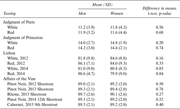
Scores were assigned in the Paris, Princeton, Lisbon, and Affairs tastings. The means and standard deviations (SDs) of women's and men's scores in each of those tastings appear in Table 2.

Table 2

H₁: Women's and Men's Scores Have Different Means and Standard Deviations

The results in Table 2 show that the means and SDs of the genders' scores are similar. However, the women's mean score is slightly higher in eight of the thirteen tastings. The random binomial probability of that observation is 0.16, and the probability of eight or more is 0.29. Further, the p-values for two-sample two-tail Student's t-tests of a difference in means show that the difference in each case is not statistically significant. Together, those results imply that H₁ is not supported. There is no statistically significant evidence that women's and men's scores have different means and SDs.

Even if the genders' score means and SDs had been identical, accepting the null hypothesis that there is no difference between women's and men's preferences could be a mistake. The hypothetical score vectors x _F  = (10, 12, 14) and x _M  = (14, 12, 10) have identical means and SDs, but they imply opposite orders of preference. The distributions of gender-specific scores may have different shapes. That possibility is tested in Section V.

V. H₂: Women and Men Have Differently Shaped Distributions of Scores

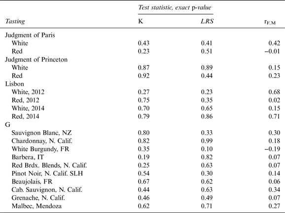
The scores or ranks assigned by individual tasters to individual wines were published for Paris, Princeton, Lisbon, and FOG. For each of those tastings, the results of two tests of a difference between the shapes of the distributions of women's and men's scores appear in Table 3.

Table 3

H₂: Women and Men Have Differently Shaped Distributions of Scores

Note: SLH, Santa Lucia Highlands.

First, the textbook-standard method of comparing the shapes of different distributions is the chi-square test advanced by Pearson (Reference Pearson1900); see, for example, Cochran (Reference Cochran1952) and goodness of fit in Khazanie (Reference Khazanie1996, 580) and Crawshaw and Chambers (Reference Crawshaw and Chambers2001, 566). From Press et al. (Reference Press, Teukolsky, Vetterling and Flannery1997, 616), with notation adapted to this article, the expression for a two-sample chi-square test of a difference in distributions appears in Equation (3). The multiplier and square-root adjustments compensate for different sample sizes, and the denominator is a sum, because the variance of a difference in independent variables is the sum of their variances. The test statistic (K) can be evaluated as having, asymptotically, a chi-square distribution. The degrees of freedom is the number of nonempty bins minus the number of constraints; thus, df = (W − 1)² when every wine is assigned every rank at least once.

(3) $$K = \mathop \sum \limits_{i = 1}^W \mathop \sum \limits_{\,j = 1}^W \displaystyle{{\left( {m_{ij}^F \left( F \right)\sqrt {M/F} - m_{ij}^M \left( M \right)\sqrt {F/M}} \right)^2} \over {m_{ij}^F \left( F \right) + m_{ij}^M \left( M \right)}}$$

The second method of testing H₂ is a variation on the Plackett-Luce LRS test of randomness employed in Section III. In Section III, the test for randomness is whether the MLEs of $\hat \rho _i $ are significantly different from $\hat \rho _i = 1/W$ . The test statistic is $LRS = \; 2 \cdot \left( {{\rm {\cal L}}_{MLE} - {\rm {\cal L}}_0} \right)$ . Here, the test is whether the MLEs of the preference probabilities for female judges ( $\hat \rho _{i,F} $ ) are significantly different from the MLEs of the preference probabilities for male judges ( $\hat \rho _{i,M} $ ). Therefore, the test statistic is $LRS = \; 2 \cdot \left( {\left( {{\rm {\cal L}}_{MLE,F} \vert\hat \rho _{i,F}} \right) + \left( {{\rm {\cal L}}_{MLE,M} \vert\hat \rho _{i,M}} \right) - {\rm {\cal L}}_{MLE}} \right)$ . In effect, this is a test of whether the observed distribution is a mixture of distinctly different gender-specific distributions.

Exact p-values for K and LRS are reported in Table 3. They are calculated for the observed F and M, using the sampling method described in Section III, from a distribution in which tasters are randomly assigned to F and M. This approach has been checked using Marden's (Reference Marden1995, 261) data for six tasters and a hypothetical set of random scores. Three of Marden's tasters have identical and materially different rankings than the other three. Assigning the three with identical rankings to F, the p-value for K is 0.06, and the p-value for LRS is <0.01. For the hypothetical set of random scores, both p-values are >0.75.

As a final check and additional comparison, the correlation coefficients (r _F,M ) between the gender-specific marginal probabilities m _ij are reported in Table 3. A simple interclass Pearson sample correlation coefficient is employed here, because potentially complex and controversial choices concerning calculation and interpretation of an intraclass correlation coefficient (ICC) are beyond the scope of this check; see Shrout and Fleiss (Reference Shrout and Fleiss1979), Cicchetti's (Reference Cicchetti2006) analysis of the Paris results, and Olkin et al. (Reference Olkin, Lou, Stokes and Cao2015, 14) concerning ICCs.

None of the exact p-values in Table 3 exceeds the widely employed 0.05 threshold of statistical significance. The r _F,M are generally low, but sixteen of the eighteen correlations are positive. The random binomial probability of that observation is <0.01. Those correlation coefficients imply that female and male judges do tend to assign high and low ranks to the same wines but that other sources of variation, such as non-gender-related idiosyncratic preferences and randomness, reduce that correlation to less than 1.0. A correlation near zero would indicate little agreement on relative preferences, and a negative correlation would indicate some aggregate differences in preferences. The results in Table 3 provide little support for H₂. In blind tastings, subject to the qualification that non-gender-related variation is substantial, women and men appear to assign about the same scores or ranks to the same wines.