1 Introduction
The ingestion of turbulence into a rotor causes unsteady loading on the blades and the formation of sound waves that radiate to the far field. The nature of this sound source has been quite well documented for simpler situations, such as where the turbulence is initially homogeneous and/or the blades see a statistically stationary flow. However, this is often not the case. Modern propulsion systems, such as the propellers of a ship or the airframe-integrated engines of an aeroplane, are designed to operate adjacent to the body of the vehicle while ingesting the inhomogeneous turbulence of its boundary layer. The substantial effects that these have on both the fluid dynamics and the acoustics of a rotor are the subject of this paper.
Early experimental and analytical work on the problem of homogeneous turbulence ingestion was carried out by Sevik (Reference Sevik1974), who studied the unsteady thrust of a rotor fully immersed in grid generated turbulence. This arrangement was modelled by assuming that the ingested turbulence was homogeneous and isotropic and governed by an exponentially decaying correlation function. The general trend of the predictions and measurements matched quite well, with the exception that the spectrum contained ‘humps’ or ‘haystacks’ at multiples of the blade rate. The reason for this mismatch was that Sevik did not consider that some turbulent structures might be cut by more than one blade, so that the fluctuating loads from blade to blade would be correlated to some extent. This effect was subsequently incorporated into analysis of the problem by Blake (Reference Blake1986), Martinez (Reference Martinez1997), Glegg & Walker (Reference Glegg and Walker1999), Joseph & Parry (Reference Joseph and Parry2001) and Atassi & Logue (Reference Atassi and Logue2009), among others.
There are two factors that contribute to blade-to-blade correlation. The first is simply the advance ratio of the rotor. If it is sufficiently small, then successive blades will cut closely spaced spiral paths through the fluid material, and thus likely meet the same turbulent structure. If the blade count is high, then the non-dimensional time delay between these cuts will be small, further increasing the correlation. The second is the distortion of turbulence as it is drawn into the rotor. In the case of a fan or compressor, the flow will accelerate towards the rotor plane, and this will tend to orient and stretch the turbulence structures in the streamwise direction, increasing the opportunity for multiple cuts by successive blades.
An extreme example of this is the ingestion of atmospheric turbulence into stationary aircraft engines, as first studied by Hanson (Reference Hanson1974). He examined the turbulence drawn into the inlet using hot-wire anemometry, and the resulting response of the blades with pressure transducers embedded within them. In this case, the substantial contraction of the flow entering the engine inlet was found to produce turbulence scales with a 400:1 streamwise to cross-stream aspect ratio and a length of the order of 100 fan diameters. These inlet vortices produced short distinct lift pulses as they were cut multiple times by the rotating blades. A similar and related phenomenon is ground vortex ingestion in stationary or near-stationary aircraft engines, studied by de Siervi et al. (Reference de Siervi, Viguier, Greitzer and Tan1982), Shin et al. (Reference Shin, Cheng, Greitzer and Tan1986), di Mare, Simpson & Sayma (Reference di Mare, Simpson and Sayma2006), and Murphy & MacManus (Reference Murphy and MacManus2011), among others. These persistent structures associated with intense stretching of fluid entering the engine originate near the ground and rise up into the fan face. In some conditions, a counter-rotating pair of vortices is observed (Murphy & MacManus Reference Murphy and MacManus2011). Organization of these structures is assisted by the presence of the shroud, which acts to separate the origin of vorticity from the rotor that ingests it. The specific situation of unbounded turbulence ingestion into a stationary engine was analysed aeroacoustically by Majumdar & Peake (Reference Majumdar and Peake1998) using rapid distortion theory, assuming initially isotropic turbulence, and by computing the sound radiated by the fan using strip theory.
Of more relevance here is the situation that occurs in cruising flight, where the stretching of turbulence approaching the fan is considerably less than for a stationary engine. While the lower levels of distortion present in this case are unlikely to result in the formation of persistent vortical structures, Majumdar & Peake (Reference Majumdar and Peake1998) showed that distortion still has an important effect on the turbulence and the resulting sound. Ingestion of moderately distorted homogeneous turbulence into a rotor has been the subject of a series of studies in the anechoic wind tunnel at the University of Notre Dame, including work by Sharpf & Mueller (Reference Sharpf and Mueller1995), Minniti, Blake & Mueller (Reference Minniti, Blake and Mueller2001a ,Reference Minniti, Blake and Mueller b ), Wojno, Mueller & Blake (Reference Wojno, Mueller and Blake2002a ,Reference Wojno, Mueller and Blake b ) and Lynch, Blake & Mueller (Reference Lynch, Blake and Mueller2005a ,Reference Lynch, Blake and Mueller b ,Reference Lynch, Blake and Mueller c ). Sharpf and Mueller studied the interaction of turbulence from three different grids with a 10 in. (254 mm) diameter four-bladed rotor. The grid turbulence was measured using hot-wire anemometry 0.6 diameters upstream of the rotor and found to be largely undistorted and of quite small scale (0.34–0.44 in. or 8.6–11 mm). Broadband sound levels radiated by the rotor were found to increase by 2 dB for every 1 % increase in turbulence level. Spectral humps associated with blade-to-blade correlations were only observed when the turbulence grid was removed and the larger (3–4 in. or 76–102 mm) eddies associated with facility background turbulence were ingested. Wojno et al. used similar turbulence generating grids and the 10-bladed rotor of Sevik’s earlier experiment. The cross-sectional structure of the undisturbed turbulence, including the lingering imprint of the turbulence grid bars, was measured in detail. Measurements were not made in the rotating frame, but measured velocity spectra were converted to the rotating reference frame assuming Taylor’s hypothesis and relying on the homogeneity of the turbulence. Predictions of the broadband sound radiated by the rotor were made using strip theory and the summation gain approach of Blake (Reference Blake1986), which accounts for the blade-to-blade correlation. Predictions showed good agreement with sound measurements, but with some differences that suggested an unaccounted for additional broadband source. Differences in the narrowband features of the spectrum also suggested that the blade-to-blade correlation was being underestimated. Minniti et al. studied a four-bladed propeller instrumented with polyvinylidene fluoride pressure sensors mounted to the blades in order to measure pressure fluctuations and their spanwise correlation. By idealizing the blade response function, they were able to infer the characteristics of the rotor inflow from the surface pressure fluctuations, an idea previously discussed theoretically by Grace, Atassi & Blake (Reference Grace, Atassi and Blake1996a ,Reference Grace, Atassi and Blake b ). Tests were made with cyclic inflow distortions to calibrate the response function of the blades, and then with grid turbulence. Inflow turbulence predictions made using the pressure response agreed well with hot-wire measurements made in the rotating frame. This was done by mounting a hot-wire probe on one of the blades with the sensor just forward of its leading edge. The far-field sound predicted from the inflow turbulence also agreed well with direct measurements. Lynch et al. focused on the response of an airfoil placed downstream of a rotor that was ingesting turbulence. They developed an empirical model of the turbulence wavenumber spectrum by assuming equal energy in all directions but with non-isotropic scales. This is done by manipulating the relationships between spectra and correlations of different components that exist in isotropic turbulence. Turbulence and mean flow measurements were made downstream of the rotor and analysed to separate the contributions from the blade wakes and the ingested turbulence. The latter showed suppression of blade normal velocity fluctuations, consistent with the rapid distortion theory predictions of Graham (Reference Graham1998).
Studies of boundary layers being drawn into rotors have tended to focus on the axisymmetric casing and hub boundary layer flows, as opposed to the thick planar boundary layer of a ship hull or an aeroplane wing. In conventional aircraft applications, inlet boundary layers tend to be thin. Particularly well known here are the experiments of Ganz et al. (Reference Ganz, Joppa, Patten and Scharpf1998) on the Boeing 18 in. (457.2 mm) fan, a high-bypass-ratio fan model with an extended inlet duct. By running the fan with and without suction to remove the 1 cm thick inlet boundary layer, Ganz et al. were able to show that the fan tip/boundary layer interaction was a significant noise source, and one that produced spectral humps indicative of blade-to-blade correlation. This specific experiment was later modelled by Glegg & Walker (Reference Glegg and Walker1999) using a von Kármán turbulence spectrum modified to account for the axial stretching of the turbulence in the approach to the fan face. Joseph & Parry (Reference Joseph and Parry2001) also modelled this experiment, but using an empirical boundary layer turbulence spectrum based on earlier work by Gavin & Lauchle (Reference Gavin and Lauchle2000). In both of these theoretical studies, the ratio of streamwise to spanwise scales in the boundary layer had to be substantially exaggerated over that measured in the experiment in order to replicate the peaked form of the measured broadband sound spectrum.
A detailed experimental study of casing boundary layer/rotor interaction has more recently been completed by Stephens & Morris (Reference Stephens and Morris2009). Here, the 10-bladed rotor of Sevik was mounted in a 206 mm diameter circular duct. Air was drawn through the duct independently of the rotor speed, allowing for variations in the flow coefficient. The rotor was placed at different distances downstream from the duct entrance, and aft of an axisymmetric bump to vary the thickness of the boundary layer interacting with the blade tips. Perpendicular-to-wall space–time correlations of the streamwise velocity component were measured in the boundary layer and used along with strip theory to determine the unsteady blade loading and thus the radiated sound, which was found to agree well with direct measurements.
The literature includes a number of studies involving hub boundary layer ingestion. Moiseev, Lakshminarayana & Thompson (Reference Moiseev, Lakshminarayana and Thompson1978) considered 10- and 17-bladed shrouded compressor rotors installed in a long annular inlet duct. The inlet was long enough that turbulent flow associated with the hub and casing boundary layers completely filled the cross-section at the rotor inflow. Measurements were performed with and without an inlet turbulence grid and with the hub boundary layer modified by adding a heavy trip or by removing the hub nose cone and adding roughness. Turbulence measurements, including circumferential correlations, were made upstream of the fan face. Sound measurements were made in an anechoic chamber containing the inlet. The grid greatly reduced turbulence integral scales, but in all cases considerable anisotropy was observed, with axial scales an order of magnitude larger than circumferential scales. Overall sound levels were found to correlate with the product of the mean-square turbulent fluctuation and the axial length scale.
While there has been little study of the acoustic effects of a nearby surface on an unshrouded rotor, there have been some studies of the fluid dynamic influence. Sato, Tasaki & Nishiyama (Reference Sato, Tasaki and Nishiyama1986) used bubble flow visualization to reveal the dynamics produced by a series of six marine propellers placed near a flat surface at a range of thrusting conditions. They found a variety of phenomena depending on the non-dimensional thrust coefficient and the blade tip clearance as a fraction of rotor diameter. At large tip clearance (greater than half the rotor diameter for the cases they studied), the presence of the wall did not substantially modify the structure of the flow passing through the rotor. As the clearance was reduced, they observed a sequence of flow patterns near the wall which they described, in order of decreasing clearance, as no-vortex reverse flow, aft vortex flow, double vortex flow, fore vortex flow and then splatter flow. These conditions were found to occur at larger tip clearance the higher the thrust coefficient. The vortex elements of these flows are commonly referred to as the propeller-hull vortex (PHV).
Martio et al. (Reference Martio, Sipilä, Sanchez-Caja, Saisto and Siikonen2011) followed Sato’s study with a URANS simulation of one of the same propellers. Calculations were performed for a large range of thrust coefficients with the tip clearance to diameter ratio fixed at 0.157. By using limiting streamlines computed on the flat surface, they could directly compare the flow patterns with the bubble flow visualization measurements from Sato et al., and found reasonable agreement at similar thrust conditions and tip gap to diameter ratios. On examining the unsteady thrust of the propeller at the highest thrust conditions, they found that it oscillated at the blade passage frequency (BPF). Significantly, they found that the PHV in the highest thrust conditions was interacting with both the blades and their tip vortices. At other, lower thrust, conditions they found that the PHV could exist without interacting with the blades.
Aeroacoustic effects of a nearby surface and the inhomogeneous turbulence of its boundary layer have been the focus of a sequence of studies in recent years of which the present paper forms a part. One of the greatest difficulties in studying inhomogeneous turbulence ingestion is in unambiguously defining the potentially very complex inflow. Morton et al. (Reference Morton, Devenport, Alexander, Glegg and Borgoltz2012) and Alexander, Devenport & Morton (Reference Alexander, Devenport, Morton and Glegg2013) solved this problem by considering the ingestion of a fully developed plane turbulent boundary layer. By measuring the complete four-dimensional space–time correlation function of the boundary layer, Morton et al. were able to define completely the linear inflow boundary condition to the rotor. Alexander et al. subsequently measured the acoustic signature of an idealized rotor (a scaled up version of Sevik’s original geometry) partially immersed in this boundary layer. Their results include far-field sound spectra that show the presence of haystacking due to correlated loading on adjacent blades as they cut through the turbulence. The haystack peaks were seen to grow in amplitude and to appear at higher harmonics of the BPF as the advance ratio was reduced. They were able to estimate some of the integral characteristics of the ingested turbulence structures by analysing their acoustic signatures – analysis that was later extended by Wisda et al. (Reference Wisda, Alexander, Devenport and Glegg2014). Far-field acoustic predictions were made for this rotor by Glegg et al. (Reference Glegg, Buono, Grant, Lachowski, Devenport and Alexander2015) using an analytical method. They used the measured undisturbed boundary layer turbulence correlations, and accounted for the inflow distortion by defining the turbulence in drift coordinates. Predictions were found to match the measurements well at low and moderate thrust; however, they deviated at high thrust and significantly underpredicted the haystacking spectral pattern in both amplitude and number of peaks.
Clues as to the possible source of disagreement were provided by the follow-up study of Alexander, Devenport & Glegg (Reference Alexander, Devenport and Glegg2017). They used blade mounted hot wires to sense directly the upwash fluctuations of the turbulence ingested into the blades. At lower thrust, consistent with Glegg et al., they found that coherence spectra of upwash velocity fluctuations measured blade to blade and spanwise agreed well with estimates based on the undisturbed boundary layer data and the trajectory of the blades. At high thrust, however, the coherence at some locations developed unexpected features, including peaks at multiples of the BPF, and upwash fluctuations close to the wall became far more intense than could be accounted for by the undisturbed boundary layer. Tuft flow visualizations on the wall revealed that the boundary layer beneath the rotor was separating in these conditions, forming (in the mean) a double vortex structure enveloping the portion of the rotor blade disk closest to the wall. Thus, it appears that, at high thrust, the acoustics of the rotor starts to become controlled by PHV effects, as opposed to the turbulence ingestion.
Alexander et al.’s findings form the starting point for the present study. We present an experimental investigation of the acoustics and aerodynamics of a rotor ingesting a turbulent boundary layer growing on a plane wall. Our study is focused on high-thrust conditions, where the inflow turbulence no longer determines the dominant radiated sound. In particular, we are interested in revealing the near-wall flow structure that becomes responsible for noise production in these conditions, as well as what happens to this flow structure and the sound as the rotor is yawed. It is important to point out that we will be discussing two distinct types of turbulence–blade interactions in this paper. The first is the rotor interaction with boundary layer turbulence, the stretched, streamwise oriented vortices and eddies of which cause a correlated response of the rotor blades at frequencies that are near multiples of the BPF. The second interaction is that of the tips of the rotor blades sweeping through or nearby an area of reversed flow, which only appears at high thrust and is likely to contain strong discrete vortical structures. We find that discrete vortical structures play a critical role in the near-wall dynamics, and that the incorporation of blade–vortex interactions with these structures is key to successfully predicting the overall noise of a rotor operating near a wall in high-thrust conditions.
2 Experimental apparatus and test conditions
This experiment was conducted in the Virginia Tech Stability Wind Tunnel (SWT) in its semi-anechoic configuration. Surface pressure, far-field acoustic and flow velocity measurements were used to gain an understanding of the interaction of the rotor with the turbulent boundary layer. Further details may be found in Murray (Reference Murray2016).
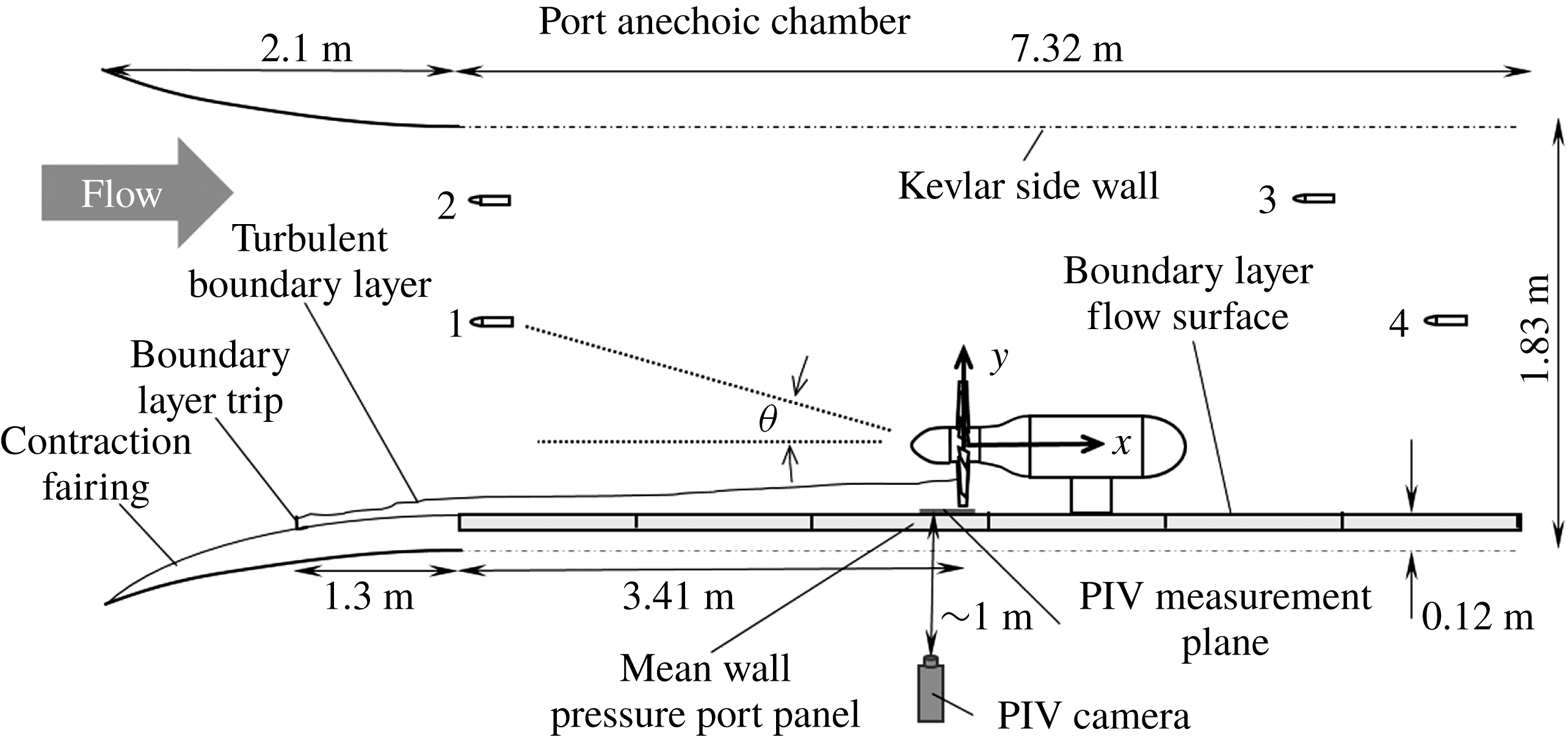
The SWT has a 1.83 m tall by 1.71 m wide by 7.3 m long semi-anechoic test section in which the experiment was performed; see figure 1. Turbulence levels in the empty test section are 0.021 % at
 $21~\text{m}~\text{s}^{-1}$
. The port sidewall of the test section is made from a tensioned Kevlar fabric that is acoustically transparent but contains the flow. Sound exiting through this Kevlar acoustic window enters an anechoic chamber, measuring 2.57 m deep by 4.21 m long, and which is anechoic down to 180 Hz. The floor and ceiling of the test section are made of 0.61 m square perforated aluminium panels with Kevlar fabric stretched over them to allow sound to pass through, where it is absorbed by acoustic wedges. The starboard wall is a hard and continuous flow surface used to grow the test boundary layer. The wall is formed from six separate Lexan panels that can be adjusted to slightly vary the width of the test section and create a zero-pressure-gradient flow in the empty test section. This configuration has been documented in several previous experiments (Awasthi Reference Awasthi2012; Forest Reference Forest2012; Morton et al.
Reference Morton, Devenport, Alexander, Glegg and Borgoltz2012; Meyers, Forest & Devenport Reference Meyers, Forest and Devenport2015). A 2.1 m long contraction fairing installed upstream of the Lexan wall mates it smoothly with the wind tunnel contraction. A single 9.5 mm tall L-bracket boundary layer trip was placed on the fairing in the contraction, 1.35 m upstream of the start of the test section and 4.76 m upstream of the rotor location, producing a turbulent boundary layer at the rotor location that was approximately 100 mm thick.
Detailed schematic of the test section set-up and instrument locations; bottom-up view. Note the location of the particle image velocimetry (PIV) camera, PIV measurement plane, microphone 1 relative to the rotor, and the location of the mean wall pressure port panel next to the rotor.

This set-up is identical to one of the configurations detailed in Morton (Reference Morton2012). Morton used two-point velocity fluctuation measurements to determine the full four-dimensional correlation function of the turbulent boundary layer over the Lexan wall in the absence of the rotor to provide an input for acoustic predictions. Boundary layer characteristics for a free-stream velocity
 $U_{\infty }$
of
 $20~\text{m}~\text{s}^{-1}$
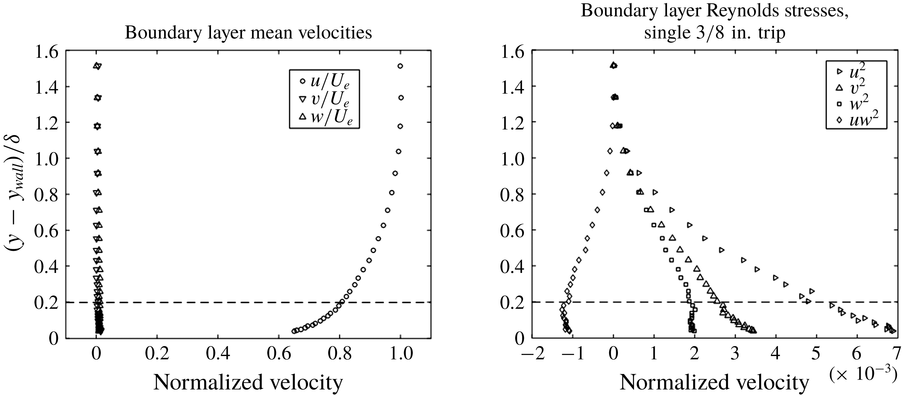
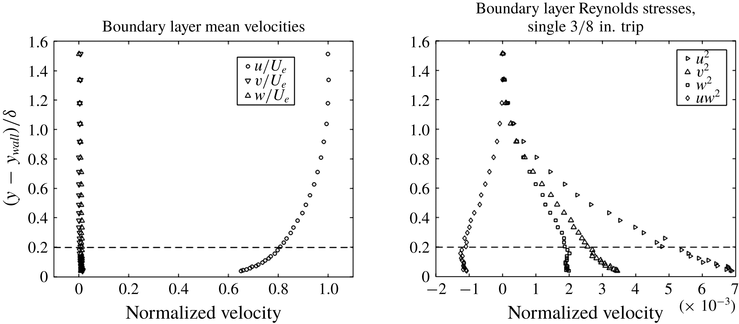
close to the rotor location, 4.72 m aft of the trip location, are listed in table 1. Corresponding mean velocity and Reynolds stress profiles are shown in figure 2. The data below documenting the zero pressure gradient of the empty test section flow were given by Morton (Reference Morton2012).
Velocity profiles measured via hot-wire anemometry from Morton (Reference Morton2012). The dashed line shows the closest approach of the rotor blades to the wall.
Boundary layer properties 4.72 m aft of the trip location, from Morton (Reference Morton2012).
 $U_{\infty }$
is the free stream velocity,
 $\unicode[STIX]{x1D6FF}$
is the boundary layer thickness,
 $C_{f}$
is the coefficient of friction on the wall,
 $\unicode[STIX]{x1D6FF}^{\ast }$
is the displacement thickness,
 $\unicode[STIX]{x1D6E9}$
is the momentum thickness, and
 $Re_{\unicode[STIX]{x1D6FF}}$
and
 $Re_{\unicode[STIX]{x1D6E9}}$
are the Reynolds number based on the displacement and momentum thickness respectively.

2.1 Rotor
The rotor design is a modified version of the 10-bladed rotor first used in Sevik’s (Reference Sevik1974) work in the four-foot water tunnel at the Ordnance Research Laboratory at Penn State. This design has been used in several studies of turbulence ingestion noise, including Wojno et al. (Reference Wojno, Mueller and Blake2002b ), Alexander et al. (Reference Alexander, Devenport, Morton and Glegg2013, Reference Alexander, Devenport and Glegg2017), Wisda et al. (Reference Wisda, Alexander, Devenport and Glegg2014, Reference Wisda, Murray, Alexander, Nelson, Devenport and Glegg2015), Glegg et al. (Reference Glegg, Buono, Grant, Lachowski, Devenport and Alexander2015) and Meyers et al. (Reference Meyers, Forest and Devenport2015), and also has a simple design and a historical record of research for comparison.
The present rotor is a left-handed 2.25 scaled version of Sevik’s initial design and has square blade tips and no skew. The blades each have a constant chord of 57.2 mm and the rotor has a total tip diameter of 457.2 mm. The diameter of the hub was expanded slightly beyond the 2.25 scale to 127 mm by removing 6.35 mm of each blade root such that the outside diameter of the rotor blades was accurately scaled. The blade pitch angle ranges from
 $21.2^{\circ }$
at the tip to
 $55.6^{\circ }$
at the root. The blade airfoil sections have a maximum thickness of 8.4 % at the tip and 9.7 % at the root, located approximately at the mid-chord. The advance ratio is typically used to characterize the thrust level of the rotor and is defined
 $J=U_{\infty }/(nD)$
, where
 $n$
is the rotation rate of the rotor in revolutions per second and
 $D$
is the rotor diameter. The design advance ratio is 1.17 and the zero-thrust-condition advance ratio is 1.44, as computed with JavaProp (Morton Reference Morton2012). A rounded nose cone with a diameter of 127 mm and a length of 216.4 mm extends in front of the blade leading edge plane. Behind the trailing edge plane, the 127 mm diameter housing extends downstream, where it gradually fairs out over 291 mm to a diameter of 219 mm to contain the drive system. A Kollmorgen AKM-64P-ACCNDA00 servo-motor powered from outside the tunnel by an S61200 servo-drive is used to power the rotor at speeds of up to 4500 RPM. The motor fairing is supported through the Lexan wall on a 76 mm thick steel strut, faired externally using foam pieces to create a symmetric airfoil section aligned with the free stream. A picture of the rotor as mounted for the experiment in the test section is shown in figure 3. The strut was adjusted to set the tip gap between the rotor and boundary layer wall to 20
 $\pm$
0.5 mm.
The Virginia Tech Stability Wind Tunnel in the semi-anechoic configuration with the rotor and wall pressure ports installed. Flow is from left to right and the rotor is yawed up at
 $+7.5^{\circ }$
.

The unyawed rotor is also used to define the test section fixed coordinate system in which measurements are presented (figure 1). The origin of the coordinate system is at the centre of the unyawed rotor disk midway between the leading and trailing edge planes. Coordinate
 $x$
is measured in the free-stream direction,
 $y$
is perpendicular to the boundary layer wall (where the wall is at
 $y_{wall}=-248.6~\text{mm}$
) and
 $z$
is spanwise across the wall so as to complete a right-handed system. Since the rotor is left handed, its rotation vector is in the positive
 $x$
direction at zero yaw. The directivity angle
 $\unicode[STIX]{x1D703}$
is measured from the negative
 $x$
axis.
The entire rotor system could be yawed with respect to the free stream, about the axis defined by the centre of the support strut, parallel to the
 $y$
axis at
 $(x,y,z)=(591.8,0,0)$
mm. Yaw angles from
 $+15^{\circ }$
to
 $-15^{\circ }$
in increments of
 $7.5^{\circ }$
were studied, where positive angles are measured as the nose of the rotor is moved in the negative
 $z$
direction.
2.2 Inflow microphones
Four Bruel & Kjaer 4190 half-inch microphones were used inside the test section to record the noise produced by the rotor at several directivity angles. The microphone arrangement inside the test section is shown in figure 1. Each inflow microphone was aligned axially with the flow and fitted with a Bruel & Kjaer UA 0386 bullet nose cap and then mounted on the top of an aerodynamically faired stand designed to produce minimal noise. The stands were bolted to the floor or ceiling and were arranged such that neither the downstream microphones nor the rotor were in the wake of any upstream microphones or stands. Inflow microphone data were recorded using a series of B&K 3050-A LXI 24-bit data acquisition systems sampling at 65 kHz for 32 s using B&K’s Pulse 14 software. Microphone 1 was the most inline and upstream microphone and had the highest signal to noise ratio, and as such all of the acoustic measurements presented in this paper will be from this microphone. Its position in metres was
 $(x,y,z)=(-2.234,0.545,-0.025)$
, implying a receiver angle of
 $\unicode[STIX]{x1D703}=13.7$
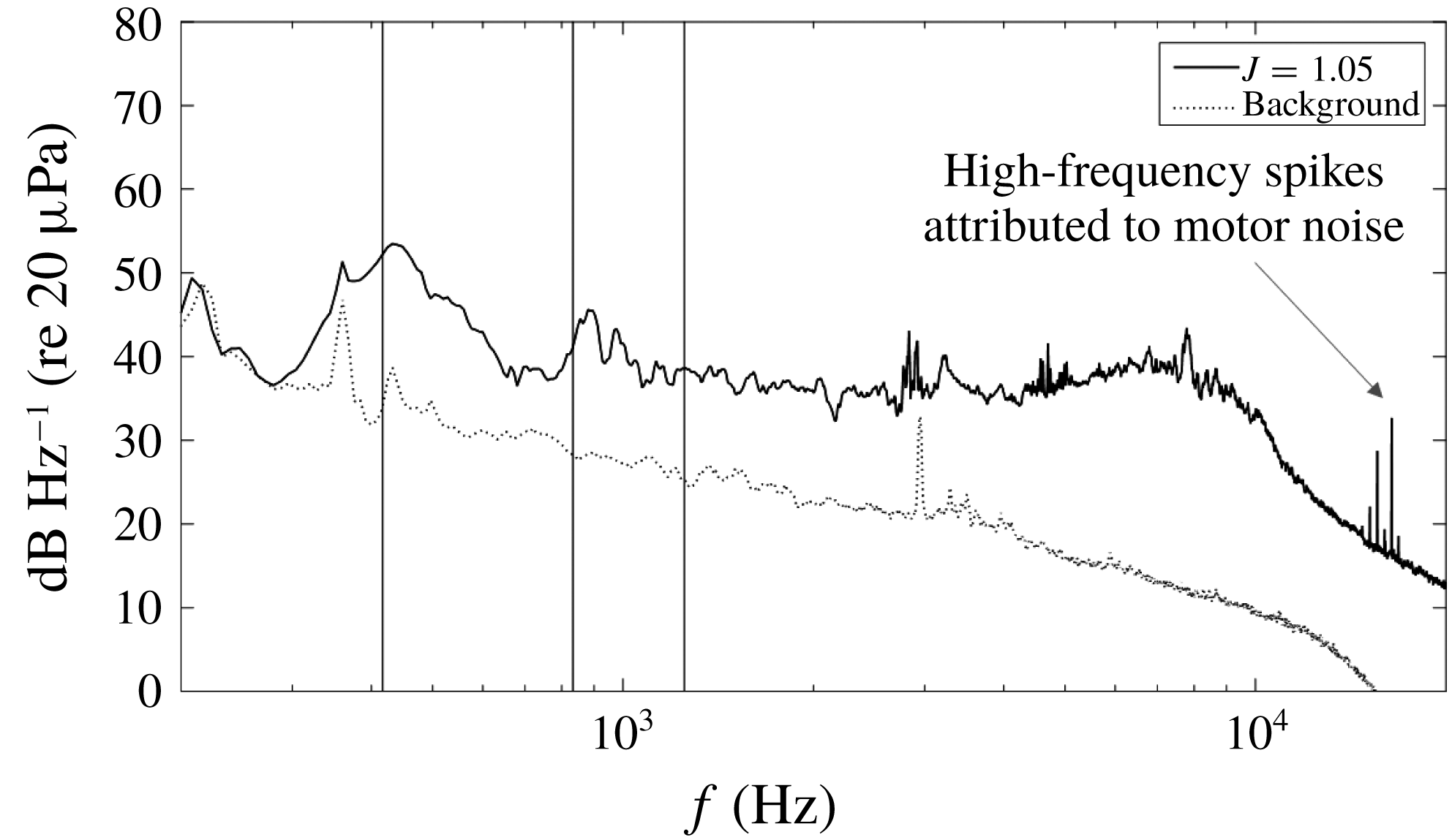
degrees from the rotor axis. The rotor system was mounted in the test section without blades, and baseline noise measurements were recorded of the electromagnetic acoustic noise and the aerodynamic noise of the motor housing at each yaw angle in order to measure the background noise not directly generated by the rotor blades. The motor was energized but not spinning during the baseline noise measurements because the system had a keyed shaft and was not able to be balanced without the blades installed. Spinning the unbalanced shaft would have created noise with a frequency at the motor rotation rate that would not be present during the actual test cases with the blades present. Figure 4 shows a typical comparison between measurements made with and without the rotor blades for the unyawed rotor at an advance ratio of 1.05. At frequencies above 300 Hz, the signal to noise ratio is at least 10 dB and in some cases above 20 dB. Background sound levels were subtracted, frequency by frequency, from sound levels with the rotor blades, except at low frequencies where the signal to noise ratio was less than 1 dB. These data were discarded. With the rotor operational, high-frequency spikes believed to be due to isolated motor tones were observed in some measurements.
Acoustic spectra from microphone 1 for
 $J=1.05$
with background to show the signal to noise ratio. Vertical lines indicate the first, second and third harmonics of the BPF for reference, 416.66, 833.33 and 1250 Hz respectively. The high-frequency spikes at 10 times the shaft rate are attributed to motor whine.

2.3 Wall pressure ports
A replaceable portion of the Lexan wall adjacent to the rotor was instrumented with 131 0.8 mm diameter pressure ports over an area located immediately beneath and upstream of the rotor; see figure 3. Ports were connected through 1.6 mm inner diameter approximately 2 m long Tygon tubing to an Esterline 9816/98RK pressure scanner with a range of
 $\pm$
10 in. of water and an accuracy of
 $\pm$
0.005 in. of water. For each run, the mean of 25 repeated pressure measurements for each port was recorded.
2.4 Particle image velocimetry system
Particle image velocimetry measurements were made in an
 $x$
–
 $z$
plane parallel to the boundary layer wall at the mid-height of the tip gap (
 $y-y_{wall}=10~\text{mm}$
). The measurement plane was illuminated with a laser sheet generated using an Nd:YAG 532 nm double pulse laser rated at 200 mJ per pulse. The laser beam was focused and expanded into a sheet with a
 $90^{\circ }$
mirror, a
 $+$
1000 mm focal length spherical lens and a
 $-$
10 mm focal length cylindrical lens before entering the wind tunnel test section through a window in its floor directed along the
 $z$
axis. The thickness of the sheet in the measurement region is estimated to have been 1–2 mm.
A LaVision Imager pro X 4M CCD camera with a resolution of
 $2048\times 2048$
pixels and an average frame rate of 3.5 Hz was used to record images of the measurement plane from beneath the rotor, through the Lexan wall (figure 1). The camera was positioned with its viewing axis aligned normal to the Lexan so as to minimize image distortion and optimize planar measurement accuracy. For each measurement, the viewing region extended 0.3
 $R$
upstream of the point of closest approach of the centre of the blade disk to the wall, 0.2
 $R$
downstream and
 $\pm$
0.5
 $R$
in the spanwise direction. Interrogation windows were sized such that the final vector field was computed with a resolution of 2.23 mm, which corresponded to an area of
 $32\times 32$
pixels.
The laser and cameras were coordinated and controlled with LaVision DaVis 8.2 software. It was used to record, preprocess the raw images, cross-correlate to compute the vector field, and postprocess the vector fields. A series of 5000 image pairs were recorded and analysed for unyawed rotor measurements. One thousand image pairs were analysed for the yawed cases. Details of the full postprocessing procedure can be found in Murray (Reference Murray2016). Postprocessing procedures filtered out vectors that were unable to be confidently determined. This left small gaps in the instantaneous velocity field which comprised on average 2 % of the part of the vector field of interest and were primarily located only directly below the blade tip. These small gaps were then filled by linear interpolation with neighbouring vectors before plotting or evaluating spatial derivatives. Phase averaging and additional postprocessing operations were then performed in Matlab. Flow in the closed-circuit Stability Tunnel was seeded directly downstream of the test section with atomized di-ethyl-hexyl-sebacat oil. The oil was atomized in a LaVision atomizer and the particles had a nominal particle diameter of
 $1~\unicode[STIX]{x03BC}\text{m}$
. Mean velocity and turbulence measurements made using the PIV system in the undisturbed turbulent boundary layer with the rotor system removed were found to be consistent with Morton’s (Reference Morton2012) results (figure 2) and those of Awasthi (Reference Awasthi2012); see Murray (Reference Murray2016).
2.5 Range of test conditions
The entire test was performed at free-stream conditions of
 $U_{\infty }=20\pm 0.15~\text{m}~\text{s}^{-1}$
and the rotor speed was varied to change its operating conditions. Measurements with the inflow microphones and mean wall pressure taps were made at 22 advance ratios ranging from
 $J=2.19$
, a heavily braking condition, to
 $J=0.58$
, a high-thrust condition, and at five yaw angles,
 $-15^{\circ }$
,
 $-7.5^{\circ }$
,
 $0^{\circ }$
,
 $+7.5^{\circ }$
and
 $+15^{\circ }$
.
The operating conditions discussed in detail in this paper form a subset of the range of conditions measured and are listed in table 2 in terms of advance ratio
 $J$
, rotor RPM, tangential blade tip velocity, free-stream relative tip velocity
 $U_{tip}$
and Reynolds number
 $Re_{tip}$
based on
 $U_{tip}$
and tip chord at zero yaw. These correspond to high thrust (
 $J=0.58$
), moderate thrust (
 $J=1.05$
) and zero thrust (
 $J=1.44$
) for all five yaw angles. Particle image velocimetry measurements were made in these conditions for yaw angles of
 $-7.5^{\circ }$
,
 $0^{\circ }$
and
 $+7.5^{\circ }$
. The full set of acoustic and mean wall pressure measurements is presented in Murray (Reference Murray2016). The focus of this paper is on the changes that take place as the rotor thrust is increased, and the fluid dynamic and acoustic characteristics of the flow that develops at high thrust.
Detailed conditions for select measurement cases.

3 Results and discussion
3.1 Unyawed rotor
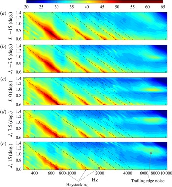
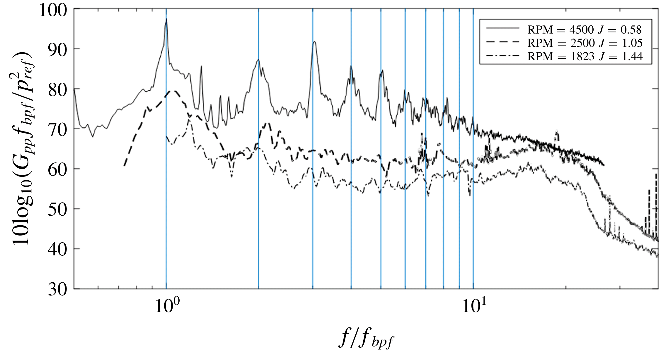
Figure 5 shows rotor noise spectra as a function of advance ratio in the form of spectral density contours. Sound spectra for the zero-, moderate- and high-thrust cases are shown in more detail in figure 6. Figure 5 and some subsequent figures to be introduced below also include measurements made with the rotor at yaw which will be discussed in the following section.
At zero yaw, the sound spectrum as a function of advance ratio, figure 5(c), reveals two different types of features: downward sloping ridges at low advance ratios at frequencies
 $f$
below 5 kHz and a high-frequency maximum centred near
 $J=0.95$
and
 $f=7.5~\text{kHz}$
. The maximum occurs only over a narrow band of advance ratios, between approximately
 $J=0.9$
and 1.05, suggesting a source strongly dependent on the blade angle of attack. While not visible in figure 5(c), a second maximum appears at higher advance ratios, centred near
 $J=1.5$
and
 $f=4~\text{kHz}$
. Both features can also be seen in the line spectra plotted in figure 6 for
 $J=1.05$
and 1.44 centred near
 $f/f_{bpf}=20$
, and Murray (Reference Murray2016) shows that they can be related using a scaling appropriate to trailing edge noise. Furthermore, they bear a close resemblance to similar spectral features seen by Hersh, Soderman & Hayden (Reference Hersh, Soderman and Hayden1974), who observed sound signatures due to laminar or transitional trailing edge vortex shedding at low, but non-zero, angles of attack and blade chord Reynolds numbers similar to those of the present experiment. Sound measurements made by Hickling (Reference Hickling2017) with the rotor positioned in the tunnel free stream show only this source.
The downward sloping ridges at lower frequencies are the haystack peaks near harmonics of the BPF. These appear only at positive-thrust conditions,
 $J<1.44$
, and become more marked as the advance ratio decreases. At the moderate-thrust-condition
 $J=1.05$
(see also figures 4 and 6), the spectrum shows two broad peaks centred just above the BPF and its first harmonic. These features are the result of ingestion of boundary layer turbulence into the rotor, an observation confirmed directly by phased array measurements presented by Wisda et al. (Reference Wisda, Murray, Alexander, Nelson, Devenport and Glegg2015) and indirectly by the absence of this noise from Hickling et al.’s (Reference Hickling2017) free-stream test.
Spectral density contour plots as a function of rotor yaw for the thrusting regime at all yaw angles examined in this experiment. Specific important spectral features are labelled in the callouts. The rotor is yawed at
 $-15^{\circ }$
in (a),
 $-7.5^{\circ }$
in (b),
 $0^{\circ }$
in (c),
 $7.5^{\circ }$
in (d) and
 $15^{\circ }$
in (e). The colour scale indicates sound pressure level in
 $\text{dB}~\text{Hz}^{-1}$
re
 $20~\unicode[STIX]{x03BC}\text{Pa}$
. Dashed lines show integer multiples of the BPF.

Representative sound spectra at, high thrust (
 $J=0.58$
), moderate thrust (
 $J=1.05$
) and no thrust (
 $J=1.44$
), normalized on BPF. The moderate-thrust condition has two haystack peaks while the high-thrust condition has 10 distinct peaks aligned with multiples of the BPF. The spikes visible between the BPF and its first harmonic at high thrust are at multiples of the rotor shaft rate and are believed to be due to mechanical noise in the rotor drive system.

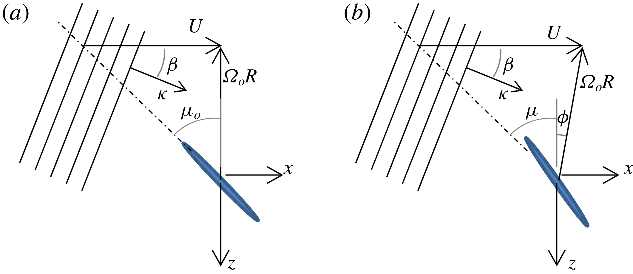
The ‘blue shifting’, or shifting of the peaks to a higher frequency, occurs because the rotating blades take a diagonal track through the downstream-convecting boundary layer turbulence. This can be analysed (see also Martinez Reference Martinez1996) by considering a single blade interacting with a harmonic component of the turbulent flow, defined in the fixed frame of reference as
 $$\begin{eqnarray}\displaystyle \boldsymbol{a}\exp (\text{i}\unicode[STIX]{x1D705}\cos \unicode[STIX]{x1D6FD}(x-Ut)+\text{i}\unicode[STIX]{x1D705}\sin \unicode[STIX]{x1D6FD}z), & & \displaystyle\end{eqnarray}$$
where
 $\unicode[STIX]{x1D705}$
is the disturbance wavenumber,
 $U$
is the speed at which the mean flow convects the gust downstream and
 $\boldsymbol{a}$
is the gust amplitude. Figure 7 illustrates a gust of this type of angle
 $\unicode[STIX]{x1D6FD}$
. Because of the boundary layer symmetry, gusts of a given amplitude will occur at positive and negative values of
 $\unicode[STIX]{x1D6FD}$
with equal probability. Moreover, since the flow is incompressible, the velocity vector fluctuation
 $\boldsymbol{a}$
will be tangent to the plane of the gust wavefronts and given by
 $\boldsymbol{a}=a(-\sin \unicode[STIX]{x1D6FD},0,\cos \unicode[STIX]{x1D6FD})$
. The gusts are convected downstream at speed
 $U$
into the rotor, and cut by blades spinning at an angular velocity
 $\unicode[STIX]{x1D6FA}_{o}$
. Since, in general, we are allowing for the rotor to be yawed at an angle
 $\unicode[STIX]{x1D719}$
, this has been included in figure 7(b).
Plan view of a rotor blade at closest approach to the wall interacting with a sinusoidal gust. (a) Zero yaw; (b) non-zero yaw.

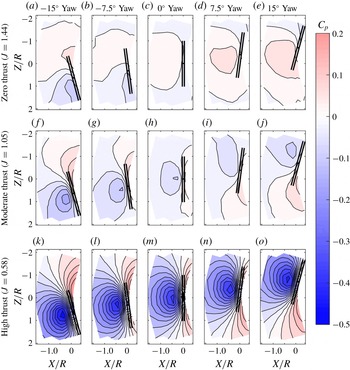
Mean wall pressure measurements as a function of rotor yaw angle for three advance ratios, zero thrust, moderate thrust and high thrust. The two parallel lines represent the projection of the rotor disk onto the wall. Note the asymmetry with respect to yaw and that it is more significant at lower rotor rotation rates.

First, we consider the case without yaw, so the blade position varies as
 $z=-R\sin (\unicode[STIX]{x1D6FA}_{o}t)$
and each blade therefore sees an upwash disturbance of the form
 $$\begin{eqnarray}\displaystyle a_{n}\exp (-\text{i}\unicode[STIX]{x1D705}\cos \unicode[STIX]{x1D6FD}(Ut)-\text{i}\unicode[STIX]{x1D705}\sin \unicode[STIX]{x1D6FD}R\sin (\unicode[STIX]{x1D6FA}_{o}t)). & & \displaystyle\end{eqnarray}$$
The important point to note here is that the unsteady loading on the blades is not periodic because the gust is convected by the mean flow at a speed that is unrelated to the blade rotation rate. The rotor blade angle
 $\unicode[STIX]{x1D6FA}_{o}t$
, measured from its closest approach to the wall, lies between approximately
 $\pm 35^{\circ }$
when the blade is immersed in the boundary layer, and so we may take
 $\sin (\unicode[STIX]{x1D6FA}_{o}t)\approx \unicode[STIX]{x1D6FA}_{o}t$
with an error of less than 10 %. The frequency magnitude of the upwash disturbance seen by the blade is then
 $$\begin{eqnarray}\displaystyle \unicode[STIX]{x1D714}=|\unicode[STIX]{x1D705}U\cos \unicode[STIX]{x1D6FD}+\unicode[STIX]{x1D705}\unicode[STIX]{x1D6FA}_{o}R\sin \unicode[STIX]{x1D6FD}|=\unicode[STIX]{x1D705}U_{rel_{o}}|\sin (\unicode[STIX]{x1D6FD}+\unicode[STIX]{x1D707}_{o})|, & & \displaystyle\end{eqnarray}$$
where
 $U_{rel_{o}}=U_{rel}|_{\unicode[STIX]{x1D719}=0}=\sqrt{U^{2}+(\unicode[STIX]{x1D6FA}_{o}R)^{2}}$
and
 $\unicode[STIX]{x1D707}_{o}=\unicode[STIX]{x1D707}|_{\unicode[STIX]{x1D719}=0}=\tan ^{-1}(U/\unicode[STIX]{x1D6FA}_{o}R)$
; see figure 7(a). We see that, except for the unlikely scenarios of
 $\unicode[STIX]{x1D707}_{o}$
approaching zero or
 $\unicode[STIX]{x03C0}/2$
(advance ratios approaching zero or infinity), the frequency is increased (blue shifted) when
 $\unicode[STIX]{x1D6FD}$
is positive and reduced (red shifted) when it is negative. Now, ignoring any out of plane velocity component, and noting that the unit vector normal to the blade surface makes an angle
 $\unicode[STIX]{x1D707}_{o}$
to the direction of the mean flow, the upwash amplitude seen by the blades is
 $$\begin{eqnarray}\displaystyle a_{n}=-a\sin (\unicode[STIX]{x1D6FD}+\unicode[STIX]{x1D707}_{o}), & & \displaystyle\end{eqnarray}$$
and thus the upwash encountered by the blade and the far-field sound will be greater for the blue-shifted frequencies than it is for the red-shifted frequencies. Since there is equal probability for a gust with positive or negative
 $\unicode[STIX]{x1D6FD}$
, it follows that the spectrum will be skewed towards higher frequencies, including the haystack peaks formed by multiple blade passages.
As the advance ratio decreases and the thrust increases, the ingested eddies become elongated and more streamwise oriented, and this narrows the haystacks. At an advance ratio of approximately 0.8, however, the number of harmonics displaying haystacks greatly increases and they take on a more tonal character, visible at
 $J=0.58$
in figure 6. Some 10 peaks are seen in this case, at multiples of the BPF, and the first and second peaks are much narrower than for
 $J=1.05$
. It is spectra of this type that Glegg et al. (Reference Glegg, Buono, Grant, Lachowski, Devenport and Alexander2015) found could not be accounted for by stretching and ingestion of the undisturbed boundary layer turbulence.
Mean wall pressure measurements also support the conclusion that a different fluid dynamic interaction is taking place at high thrust. Contours of mean pressure for the unyawed rotor at the representative advance ratios are shown in figure 8(c,h,m). In the perspective of figure 8, the rotor blade tips move through the boundary layer in the negative
 $z$
direction, approaching the wall at positive
 $z$
(the downstroke side) and leaving it at negative
 $z$
(upstroke side). The pressure distributions are nearly symmetric across the rotor axis, with a slight skewing of the features towards the upstroke side for the zero-thrust condition (figure 8
c), although the rotor has a relatively weak impact on the wall pressure field at this condition. In the moderate-thrust case,
 $J=1.05$
, figure 8(h), the near-wall flow approaching the rotor from upstream first experiences a favourable pressure gradient as it is drawn towards the upstream face of the rotor. However, close to the rotor face, fluid starts to be drawn away from the wall also, resulting in a pressure minimum followed by an adverse pressure gradient and deceleration near the wall. In figure 8(h), the pressure minimum is reached at
 $x/R=$
 $-$
0.3, where
 $C_{p}=-0.07$
, and the subsequent adverse pressure gradient
 $\unicode[STIX]{x2202}C_{p}/\unicode[STIX]{x2202}(x/R)$
reaches a maximum of 1.37 near
 $x/R=0.081$
on the centreline. The measured mean wall pressure is highest, and the near-wall velocity lowest, directly downstream of the centre of the rotor at
 $x/R=0.08$
, where
 $C_{p}=0.095$
.
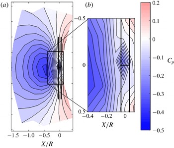
Mean wall pressure field for the highest-thrust case (a) with an expanded view of the second low-pressure region in the tip gap (b).

As the rotor thrust is increased to the high-thrust condition (figure 8
m), the flow acceleration ahead of the rotor intensifies and the resulting pressure minimum on the wall deepens. At
 $J=0.58$
, the maximum
 $C_{p}$
value upstream of the rotor is
 $-$
0.36, approximately five times that seen in the moderate-thrust case. Not surprisingly, there is a corresponding increase in the adverse pressure gradient experienced at the wall as the flow enters the tip gap,
 $\unicode[STIX]{x2202}C_{p}/\unicode[STIX]{x2202}(x/R)$
, reaching a maximum of 4.69 at
 $x/R=0.08$
for
 $J=0.58$
. However, in this high-thrust case, a second pressure minimum appears, formed immediately under the rotor disk, where the pressure coefficient drops once more, to
 $-$
0.27. This region, highlighted in figure 9, is sufficiently small to only span one of the wall pressure taps, and thus its diamond shape is a consequence of the measurement resolution rather than flow details. This feature was also seen with the rotor yawed, where the minimum was detected by different taps, making it unlikely to be an instrumentation error. Indeed, the appearance of this second pressure minimum is symptomatic of a change in the structure of the velocity field under the rotor.
Mean velocity contour levels and vectors through the tip gap for two thrust conditions (
 $J=1.05$
, moderate thrust, and
 $J=0.58$
, high thrust) at three rotor yaw angles (
 $-7.5^{\circ }$
,
 $0^{\circ }$
and
 $+7.5^{\circ }$
).

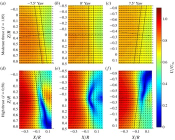
Mean velocity measurements made in a plane parallel to the wall at the mid-height of the tip gap are shown in figure 10(b,e). In the moderate thrust case, the flow is almost unidirectional and slows by approximately
 $0.2U_{\infty }$
as it passes under the rotor blade tips; see figure 10(b). The velocity changes and flow pattern appear to be consistent with the mean pressure field (figure 8
h), as they do for the zero-thrust case (Murray Reference Murray2016). In the high-thrust case, however, the slowing of the flow approaching the rotor becomes more marked and an arc-shaped region of separation forms under the blade disk; see figure 10(e). On either side of the arc, strong counter-rotating cells, centred at approximately
 $z/R=0.13$
and
 $-$
0.17, feed reversed flow into the separation. The flow travels upstream to a stagnation point formed on the axis of symmetry near the blade leading edge plane. It is clear that this reversed flow, which has a maximum mean velocity magnitude equivalent to 43 % of the free stream, is responsible for the second pressure minimum seen at the wall. The separation region is slightly offset towards
 $-z$
on the upstroke side of the centreline.
The counter-rotating cells seen in figure 10(e) bear quite a close resemblance to flow patterns seen in the ground vortex study of Murphy & MacManus (Reference Murphy and MacManus2011), at their lowest inlet velocity ratio. They studied the ingestion of a plane boundary layer into a circular inlet through PIV measurements made in a plane parallel to the wall at the mid-height of the gap between the wall and the lower inlet lip. At conditions roughly comparable to the present high-thrust case (gap equivalent to 25 % of the inlet diameter
 $D$
, inlet boundary layer displacement thickness of
 $0.11D$
and ratio of inlet to free-stream velocity of 4.4), a mean flow counter-rotating circulation pattern with the same orientation, sense and approximate scale as that of figure 10(e) was observed. There are some important differences here though. Most significantly, no rotor was present in Murphy and McManus’s experiment, and thus the vortex structures were generated only by lifting off the wall and stretching of the boundary layer turbulence generated by steady inlet suction. In the present experiment, the separated flow forms right at the rotor disk, and its structure is thus at least as much the result of the local unsteady influence of the repeated passage of individual blades as it is of the overall streamline contraction of the flow entering the rotor. A consequence of this, to be discussed further below, is that the instantaneous vortical structures associated with the separation are extremely unsteady and not persistent in the manner of ground vortices.
The mean flow reversal observed at high thrust is caused by the presence of the wall. The wall constrains the contraction of the stream tube of air entering from upstream as compared with an unobstructed rotor. This starves the blade disk of fluid on the wall side, creating a larger pressure differential across the blade disk there that results in a flow reversal in the rotor–wall gap. Phase averaging of the velocity field with respect to the rotor position is revealing in this case. This was achieved by sorting the velocity field measurements into bins, each representing two degrees of blade rotation and each containing approximately 200 measurements. The point closest to the wall is defined as
 $0^{\circ }$
phase. The blade closest to the wall is approaching the wall at negative phase angles and retreating from it at positive phase angles. Three evenly spaced and representative phase angles centred at
 $-12^{\circ }$
,
 $0^{\circ }$
and
 $12^{\circ }$
are shown for the unyawed
 $J=0.58$
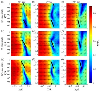
case in figures 11(b), 11(e) and 11(h) respectively. At lower thrust conditions, these phase averages show regions of lower-velocity fluid trailing from the blades, consistent with motion induced by the trailing blade tip vortices (Murray Reference Murray2016). In the high-thrust case, however, the flow is dominated by the bulk flow reversal and these tip vortex features are not visible. Instead, the position of the counter-rotating cells in the measurement plane fluctuates as the blade passes by the wall. As the blade reaches its closest approach to the wall at
 $z=0$
, figure 11(e), the flow reversal is strengthened by a higher-velocity region of fluid in the tip gap travelling perpendicular to the blade chord and displacing part of the stagnation region. This high-velocity region of fluid is probably caused by the pressure differential between the pressure and suction sides of the blade. As the blade moves to negative
 $z$
and away from the wall, figure 11(h), the higher-velocity region of reversed flow remains near
 $z=0$
. Thus, the phase averaged results suggest that the flow reversal pattern observed in the mean tends to be reinforced by the passage of the blade tips.
Evenly spaced and representative phase averaged velocity fields for the high-thrust condition (
 $J=0.58$
) of the rotor for each yaw case considered. The black ovals are the projection of the blade tips into the measurement plane.

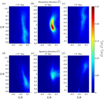
The Reynolds stress fields for the unyawed case, figure 12(b,e), quantify just how unsteady this process is. The streamwise and spanwise normal stresses,
 $\overline{u^{2}}$
and
 $\overline{w^{2}}$
, reach respective maxima of 25 %
 $U_{\infty }^{2}$
and 10 %
 $U_{\infty }^{2}$
in the measurement plane, some 40 times the levels in the undisturbed boundary layer. The
 $\overline{u^{2}}$
component is largest in a crescent-shaped region between
 $z/R=-0.2$
and
 $+0.2$
, with the highest turbulence levels occurring towards the downstroke side at
 $z/R=0.07$
. The
 $\overline{w^{2}}$
component is largest in a similarly located but elliptically shaped region. Again, the highest turbulence levels are seen towards the downstroke side. The skew of the peak Reynolds stress components to the downstroke side agrees with on-blade hot-wire measurements for this rotor published by Alexander et al. (Reference Alexander, Devenport and Glegg2017). These showed the intensity of upwash velocity fluctuations encountered by the blades to be higher on the downstroke than on the upstroke side. Taken together, these results indicate that the unsteady aspects of the flow reversal do not behave symmetrically and that the direction of rotation of the rotor is significant. This is a consequence of the increased prevalence of intense vortical structures formed on the downstroke side, as will be discussed in § 3.4.
Streamwise and spanwise components of the normal turbulence stresses in the measurement plane at the highest-thrust condition,
 $J=0.58$
, for all of the yaw cases examined,
 $-7.5^{\circ }$
,
 $0^{\circ }$
and
 $+7.5^{\circ }$
.

Representative instantaneous velocity vectors and associated vorticity contours fields for the high-thrust case (
 $J=0.58$
). Panels (a–c) and (e) show examples of commonly observed flow patterns in the unyawed case and (d,f) show typical flow structures as the rotor is yawed. Panels (a,b) show examples for the unyawed case of the most commonly observed structure, a single strong counterclockwise vortex, and (e) shows the second most commonly observed structure, a pair of counter-rotating vortices. Panel (c) shows, for the unyawed case, an example of no-vortex flow reversal, and (d,f) show the same for the negative and positive yawed cases respectively.

Consistent with the high Reynolds stress values in the tip gap, the instantaneous flow in the rotor–wall gap at high thrust (
 $J=0.58$
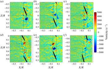
) was found to be highly unsteady. Several example flow patterns are shown in figure 13. The most commonly observed flow feature was flow reversal with a single strong vortex visible, figures 13(a) and 13(b). The second most common pattern was flow reversal with a double vortex pair, figure 13(e), and the third of the commonly observed flow patterns was flow reversal without any strong vortices clearly present, figure 13(c). A very small percentage had three or more strong vortices. None of the instantaneous measurements closely resemble the time or phase averaged results. This suggests that the presence of the counter-rotating cells is highly unsteady and intermittent, since a single vortex is also frequently observed. The instantaneous flow in the tip gap appears to take on several of the characteristic patterns documented in Sato et al. (Reference Sato, Tasaki and Nishiyama1986), including the double vortex, the fore or aft vortex and the splatter flow.
The vortices of figure 13 are visible in the measurement plane because they are oriented approximately perpendicular to the wall. The existence and location of these vortices appears to be consistent with the URANS simulations of the propeller-hull–vortex interaction computed by Martio et al. (Reference Martio, Sipilä, Sanchez-Caja, Saisto and Siikonen2011). Most significantly, they found that at a sufficiently low advance ratio, the rotor blades would interact with vortices originating from the separation region near the wall. These vortices would probably be lifted up into the rotor disc by the circulation around the blade tips. We would expect separation vortices with the same sense as the bound circulation on the blades to be intensified in this process. The sweeping of the separation vortices up into the blade disk would set up a complicated blade–vortex interaction, but parallel components of the blade–vortex interactions would be particularly efficient acoustically and thus expected to dominate the far-field sound. This hypothesis will be investigated further in § 3.4.
3.2 Effects of rotor yaw
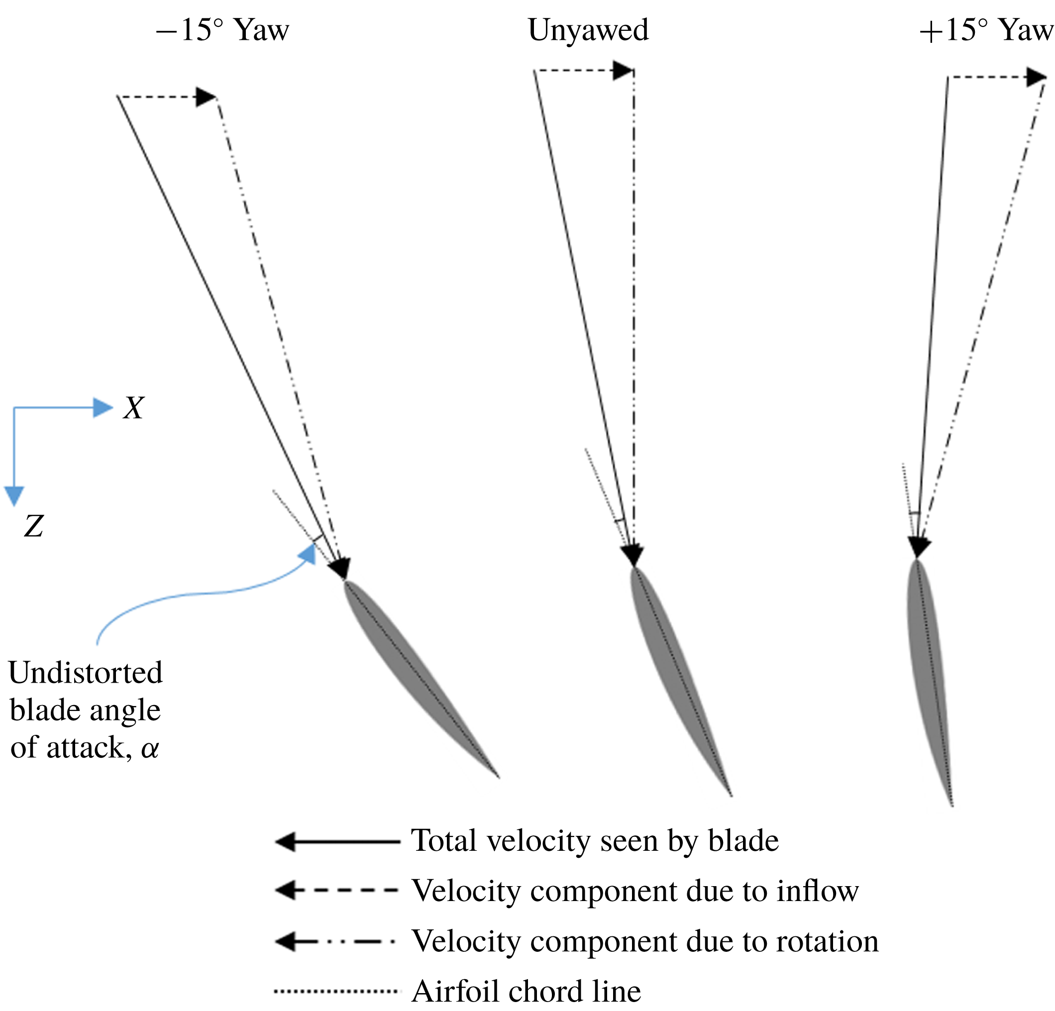
Yawing of the rotor with respect to the free stream creates operating conditions that change for the blades over the course of each rotation. Considering the blade at the point closest to the wall, figure 14, positive yaw (which turns the blade disk about the
 $y$
axis, figure 1) decreases the geometric angle of attack of the blades as they pass through the boundary layer adjacent to the wall, and negative yaw increases it. The reverse changes occur on the side of the blade disk away from the wall, but this part of the rotor is in clean flow and is not involved in the generation of turbulence ingestion or wall-separation noise. In the moderate-thrust case (
 $J=1.05$
), yawing the rotor from
 $+15^{\circ }$
to
 $-15^{\circ }$
creates an increase of
 $1.49^{\circ }$
in the geometric angle of attack at the point closest to the wall, approximately equivalent to a reduction in advance ratio to 0.98. In the high-thrust case (
 $J=0.58$
), yawing of the rotor over the same range only creates an increase of
 $0.48^{\circ }$
. This difference is due to the increased dominance of the rotational velocity component on the blade angle of attack.
Velocity triangle of the motion of the blade relative to the inflow air when it is closest to the wall for the range of yaw angles considered in this experiment, drawn relative to the orientation of the fixed coordinate system, shown to the left.

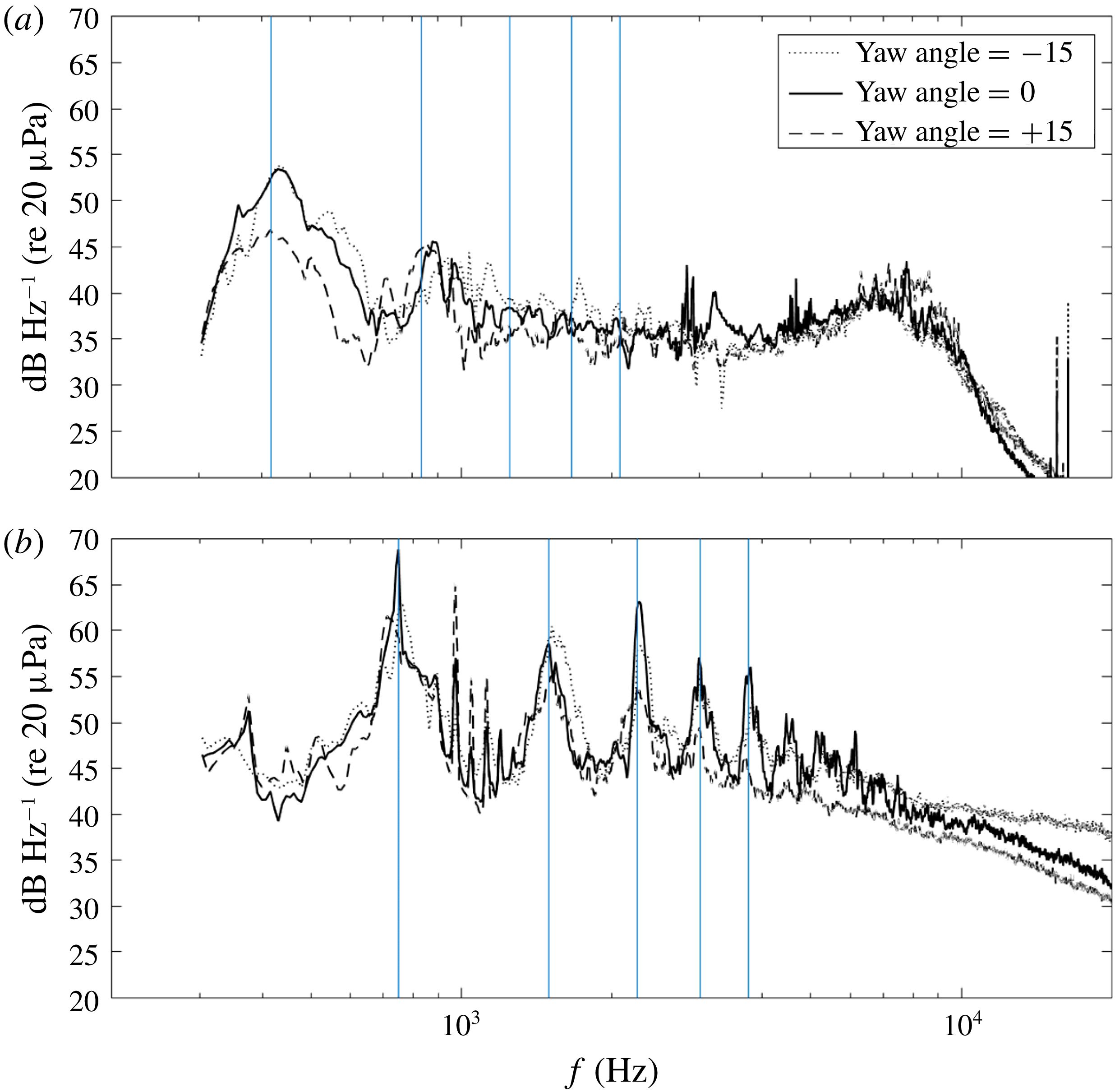
Comparison of far-field acoustic spectra as a function of yaw. Panel (a) (
 $J=1.05$
) shows the spectral pattern typical of operating conditions where the flow is unseparated, namely a monotonic increase in the haystacking with reduction in rotor yaw angle. Panel (b) (
 $J=0.58$
) shows the typical spectral pattern found when the operating conditions induce separation below the rotor. In this case, the unyawed case has the strongest haystacking and it decreases as the rotor is yawed away from the centreline in either direction.

The effects of yaw on the rotor acoustic signature are shown in figures 5 and 15. The high-frequency spectral hump seen centred around 7.5 kHz,
 $J=0.95$
and attributed to transitional trailing edge vortex shedding becomes more diffuse as the rotor is yawed. This is consistent with the yawed rotor blades now experiencing a range of angles of attack as they pass through the free stream, and the fact that this phenomenon is expected to be angle of attack sensitive. The haystack features show some distinct effects of yaw. Excluding the unyawed case, an increase in yaw angle results in a monotonic weakening of the haystacks (e.g. figure 5). The unyawed case does not fit this trend, at least at low advance ratios
 $J<0.65$
where the sound spectra show more clearly defined haystacks that extend to higher harmonics than at any other yaw angle. This effect is shown in more detail for
 $J=0.58$
in figure 15(b). At this low advance ratio, the spectra for all yaw angles have the tonal character seen in the unyawed case. However, the peaks at the BPF are loudest for the unyawed rotor, with sound levels some 5 dB and 7 dB over those seen for the
 $-15^{\circ }$
and
 $+15^{\circ }$
yaw respectively. As will be shown below, this is because rotor yaw substantially changes the structure of the separated flow at the wall generated at high thrust.
In addition to the above effects, yaw also influences the frequency bias of the haystacks. Referring to figure 7(b) and (3.3) and (3.4), we note that with yaw the blade location is given by
 $x=R\sin \unicode[STIX]{x1D719}\sin (\unicode[STIX]{x1D6FA}_{o}t)$
and
 $z=-R\cos \unicode[STIX]{x1D719}\sin (\unicode[STIX]{x1D6FA}_{o}t)$
, and so the frequency of the upwash gust encountered by the blade is
 $$\begin{eqnarray}\displaystyle \unicode[STIX]{x1D714} & = & \displaystyle |\unicode[STIX]{x1D705}(U-\unicode[STIX]{x1D6FA}_{o}R\sin \unicode[STIX]{x1D719})\cos \unicode[STIX]{x1D6FD}+\unicode[STIX]{x1D705}\unicode[STIX]{x1D6FA}_{o}R\cos \unicode[STIX]{x1D719}\sin \unicode[STIX]{x1D6FD}|\nonumber\\ \displaystyle & = & \displaystyle \unicode[STIX]{x1D705}U_{rel}|\sin (\unicode[STIX]{x1D6FD}+\unicode[STIX]{x1D707})|,\end{eqnarray}$$
where
 $U_{rel}=\sqrt{U^{2}+(\unicode[STIX]{x1D6FA}_{o}R)^{2}-2U\unicode[STIX]{x1D6FA}_{o}R\sin \unicode[STIX]{x1D719}}$
and
 $\unicode[STIX]{x1D707}=\tan ^{-1}([U-\unicode[STIX]{x1D6FA}_{o}R\sin \unicode[STIX]{x1D719}]/\unicode[STIX]{x1D6FA}_{o}R\cos \unicode[STIX]{x1D719})$
. The blade normal is also rotated by an amount that is equal to the yaw angle, and so the gust amplitude becomes
 $$\begin{eqnarray}\displaystyle a_{n}=-a\sin (\unicode[STIX]{x1D6FD}+\unicode[STIX]{x1D707}-\unicode[STIX]{x1D719}). & & \displaystyle\end{eqnarray}$$
Since, for realistic advance ratios,
 $\unicode[STIX]{x1D707}$
decreases with
 $\unicode[STIX]{x1D719}$
, the effect of positive yaw is to reduce the frequency and the gust intensity, reducing the blue shifting. In contrast, the blue shifting will be increased for negative yaw. This is exactly what is seen in the spectra of figures 5 and 15(a).
The effects of rotor yaw and advance ratio on the pressure coefficient distribution on the wall and the mean flow field above it in the middle of the tip gap are shown in figures 8 and 10. The geometric angle of attack effects described above lead to asymmetry in the flow patterns produced at positive and negative yaw angle. This is most visible in the mean pressure contours at nominal zero thrust (figure 8 a–e). Unyawed (figure 8 c), the blade disk actually produces a slight flow blockage and thus a shallow maximum in the wall pressure ahead of the rotor. However, at negative yaw (figure 8 a,b), the local angle of attack of the blades near the wall is increased, developing thrust and generating a low-pressure region ahead of the rotor. The converse is true for positive yaw (figure 8 d,e), where the negative angle of attack of the blades close to the wall leads to a slowing of the flow ahead of the rotor and thus a more distinct pressure maximum than that seen in the unyawed case. Although not shown here, the mean flow at the zero-thrust condition confirms these effects and indicates that yawing of the rotor causes a decrease and increase at negative and positive yaw respectively in the blockage effect caused by the rotor near the wall.
A similar effect happens in the moderate-thrust case. Yawing of the rotor in the negative direction causes a larger low-pressure region upstream of the rotor when compared with the unyawed case, figure 8(f) versus 8(h). This implies that the rotor thrust near the wall is increased as the local blade angle of attack there is increased. This is also supported by the larger velocity differential through the tip gap when compared with the unyawed case, figure 10(a) versus 10(b). The opposite is then true for the positive-yaw case, figure 8(h) versus 8(j) and figure 10(b) versus 10(c). The maximum mean velocity differential in the measurement region across the blade disk is 27 %, 20 % and 15 %
 $U_{\infty }$
for yaw angles of
 $-7.5^{\circ }$
,
 $0^{\circ }$
and
 $7.5^{\circ }$
respectively. The slowing of fluid through the tip gap for the thrusting case is due to the contraction of the stream tube of the flow passing through the rotor disk above. Murray (Reference Murray2016) showed that, in the phase locked view, this deceleration is organized by the influence of the trailing blade tip vortices.
Results for the same yaw angles at the highest-thrust condition reveal a very different story. The mean wall pressure distribution, figure 8(k–o), shows a strong low-pressure area directly upstream of the rotor that remains almost fixed relative to it with yaw angle. This region is centred 0.3–0.4
 $R$
upstream of the rotor disk along its axis. The magnitude of the minimum pressure coefficient here is slightly larger for the yawed cases than the unyawed ones:
 $-$
0.46 and
 $-$
0.40 for
 $-15^{\circ }$
and
 $+15^{\circ }$
yaw respectively compared with
 $-$
0.37 with no yaw. The second wall pressure minimum that was observed under the rotor disk at high thrust in the unyawed case, and associated with the separation and reversed flow observed here, is also seen in the yawed cases of figures 8(k–o). In the unyawed case, this feature was observed for all
 $J<0.62$
, suggesting that separation and reversed flow was initiated at
 $J\approx 0.62$
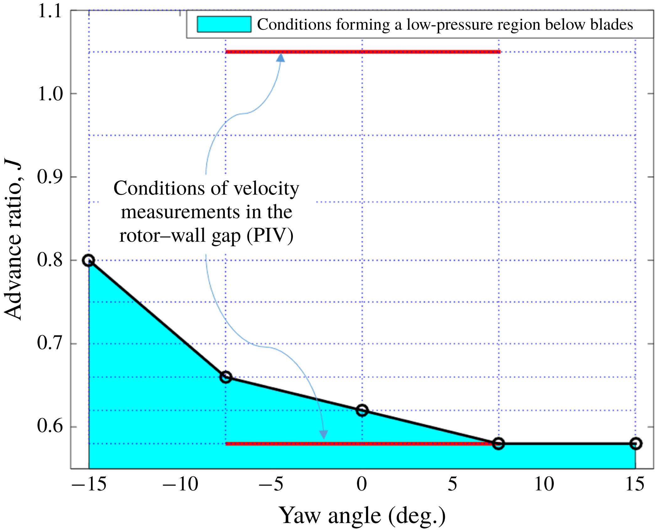
. By examining the pressure distributions measured as a function of both advance ratio and yaw, it was possible to identify the boundary between separated and unseparated rotor operation as a function of yaw angle. This boundary is shown in figure 16. We see that separation from the wall occurs more readily when the rotor is placed at a negative yaw angle, with separation occurring at
 $J\approx 0.8$
and 0.66 for yaw angles of
 $-15^{\circ }$
and
 $-7.5^{\circ }$
respectively, but is harder to induce at positive angles, with separation initiated at
 $J\approx 0.58$
for
 $7.5^{\circ }$
and
 $15^{\circ }$
. This is consistent with the fact that negative yaw increases the angle of attack and therefore thrust over the bottom portion of the rotor disk that is immersed in the boundary layer.
Yaw and advance ratio conditions at which pressure gradient reversal was observed on the wall below the rotor. The dotted horizontal and vertical lines indicate yaw angle and advance ratio conditions from the test matrix, and the filled region represents the conditions where pressure gradient reversal was observed. It should be noted that negative yaw increases the local blade angle of attack near the wall.

Mean velocity measurements show that the flow reversal pattern changes dramatically when the rotor is yawed. With the rotor unyawed, figure 10(e), the flow reversal occurs almost symmetrically about the
 $z/R=0$
line. However, the yawing of the rotor, figure 10(d,f), skews the flow, redirecting the flow reversal sideways to form a crossflow immediately downstream of the rotor blades, directed towards the downstream side of the rotor. The approximate peak magnitudes of the measured mean crossflow velocities are 80 %
 $U_{\infty }$
and 60 %
 $U_{\infty }$
for the negative and positively yawed cases respectively, compared with a maximum back flow velocity of 42 %
 $U_{\infty }$
for the unyawed case. The crossflow feeds a stagnation region that extends under the rear part of the downstream side of the rotor and trails off out of the measurement region. This is in contrast to the unyawed case, where the flow reversal is associated with a small stagnation region directly under the centre of the rotor. As with the mean wall pressure measurements, the location of the features in the crossflow pattern appears to be very closely symmetric with respect to yaw, although the crossflow is slightly stronger in the negative-yaw case.
The effects of yaw on the phase averaged velocity fields in the high-thrust case are shown in figure 11. In the
 $-7.5^{\circ }$
case, figure 11(a,d,g), the separation region is on the downstroke side of the blades and appears to be swept along with each blade tip as it passes over the wall. In contrast, in the
 $+7.5^{\circ }$
case, figure 11(c,f,i), the blade appears to have minimal effect on the tip gap flow before it reaches the point closest to the wall. At the point closest to the wall, however, the blade appears to induce a separate separation region in the centre of the tip gap which is then swept up to combine with the main separation region located under the upstroke side of the blades and seen in the mean flow for this case. The phase averages for the yawed cases do not show the high-velocity region of fluid in the tip gap when a rotor blade is closest to the wall that is seen in the unyawed case. The crossflow patterns produced by the rotor at yaw also appear to be relatively independent of the blade phase, unlike the flow reversal below the blades in the unyawed case. This supports the inference made from a comparison of the far-field spectra at different yaw angles that the rotor blades in the unyawed case interact with the flow reversal more strongly than in the yawed cases.
Example instantaneous velocity fields at the highest-thrust condition,
 $J=0.58$
, for each yaw case considered, plotted on contours of the
 $Q$
-criterion. These are the same velocity fields as shown in figure 13(d,f) to show the effectiveness of the
 $Q$
-criterion in identifying vortex formations in the velocity fields. Small areas of missing data, generally close to the blade position, were linearly interpolated over, as was required for the computation of a continuous
 $Q$
-criterion.

The effects of yaw on the Reynolds stress distributions are shown in figure 12. The regions of highest Reynolds stress in both yawed and unyawed cases correspond closely to the separation regions found in the mean flow fields, figure 10(d–f). However, the intensity of the velocity fluctuations is much lower when the rotor is yawed, particularly in the streamwise direction. The
 $\overline{u^{2}}$
component reaches peak values of 8.5 %
 $U_{\infty }^{2}$
and 7.5 %
 $U_{\infty }^{2}$
for the
 $-7.5^{\circ }$
and
 $+7.5^{\circ }$
yaw cases respectively compared with 25 %
 $U_{\infty }^{2}$
in the unyawed case. For
 $\overline{w^{2}}$
these values are 9.1 %
 $U_{\infty }^{2}$
and 6.4 %
 $U_{\infty }^{2}$
in the
 $-7.5^{\circ }$
and
 $+7.5^{\circ }$
yaw cases respectively, compared to 10.7 %
 $U_{\infty }^{2}$
in the unyawed case. The lower turbulence stresses are accompanied by differences in the instantaneous flow field. Examples of common instantaneous flow patterns seen in the tip gap region as a function of yaw angle are shown in figure 13(a–f). At zero yaw, figures 13(a–c) and 13(e), the flow was found to be dominated by a single vortex or pair of counter-rotating coherent vortices in over three quarters of the measurements made at this condition. With the rotor yawed, however, the most common flow pattern observed was that of a single vortical structure rotating clockwise when the rotor was yawed in the negative direction and counterclockwise when the rotor was yawed in the positive direction. Examples of these structures are seen at (
 $x,z$
)
 $=$
(
 $-0.03R$
, 0.19
 $R$
) and (
 $-0.01R$
,
 $-0.35R$
) in figures 13(d) and 13(f) respectively. Flow patterns that involved at least one strong vortex were only observed for just over a third of the measurements in the
 $-7.5^{\circ }$
and
 $+7.5^{\circ }$
cases. Despite the lack of identifiable vortical structure in the rest of the yawed measurements, the crossflow near the wall and downstream of the rotor disk was clearly visible in each measurement.
3.3 Vortex identification and quantification in the instantaneous velocity fields
The presence, relative strength and location of the vortices observed in the high-thrust
 $J=0.58$
case were quantified. The first step was to identify them using the
 $Q$
-criterion of Hunt, Wray & Moin (Reference Hunt, Wray and Moin1988) and Haller (Reference Haller2005). The
 $Q$
-criterion is a measure of the relative strengths of the vorticity tensor (
 $\unicode[STIX]{x1D734}$
) and strain rate tensor (
 $\unicode[STIX]{x1D64E}$
), defined as
 $$\begin{eqnarray}\displaystyle Q={\textstyle \frac{1}{2}}(|\unicode[STIX]{x1D734}|^{2}-|\unicode[STIX]{x1D64E}|^{2})>0, & & \displaystyle\end{eqnarray}$$
where, for the planar velocity fields measured beneath the rotor,
 $|\unicode[STIX]{x1D734}|^{2}=(\unicode[STIX]{x2202}u/\unicode[STIX]{x2202}z-\unicode[STIX]{x2202}w/\unicode[STIX]{x2202}x)^{2}$
and
 $|\unicode[STIX]{x1D64E}|^{2}=(\unicode[STIX]{x2202}u/\unicode[STIX]{x2202}x)^{2}+(\unicode[STIX]{x2202}w/\unicode[STIX]{x2202}z)^{2}+1/2(\unicode[STIX]{x2202}u/\unicode[STIX]{x2202}z+\unicode[STIX]{x2202}w/\unicode[STIX]{x2202}x)^{2}$
. Where
 $Q>0$
, the vorticity tensor is dominant over the strain tensor, indicating organized vortical flow in this region. Contours of
 $Q$
are shown in figure 17 for the three instantaneous velocity fields shown in figure 13(d–f). These examples illustrate the utility of the
 $Q$
-criterion in identifying vortical structures in complex planar velocity fields. Three specific challenges were overcome in developing an automated method of identifying vortices and extracting their centre locations based on local maxima of the
 $Q$
-criterion scalar field: (1) establishing a lower limit for what qualified as a vortex, (2) ensuring that vector fields without any strong vortices were flagged as such and (3) ensuring that two adjacent local maxima in the
 $Q$
-criterion that were part of the same vortex were only flagged as one.
The first and second challenges were solved by performing a trade study on a subset of 26 velocity fields from the unyawed measurements, which all together only had one or two strong vortices but a large number of weaker vortical formations. The study was run to identify the discrimination level that showed the fewest false positives while still identifying the strong vortices in this example data set. This level, of
 $1.5\times 10^{6}~\text{s}^{-2}\equiv 784U_{\infty }^{2}/R^{2}$
, was approximately 30 % of the maximum value typically seen at the centre of such vortices.
The third challenge was overcome by smoothing the
 $Q$
-criterion data, before the discrimination level was applied and the maxima identified, using a square kernel 11 mm in edge. This distance, equivalent to 2.4 % of the rotor radius and 11 % of the boundary layer thickness, was roughly equal to the typical core size (10 mm) of the vortices observed in the raw instantaneous flow fields. After smoothing, maxima closer than this distance were assumed to be identifying the same vortex.
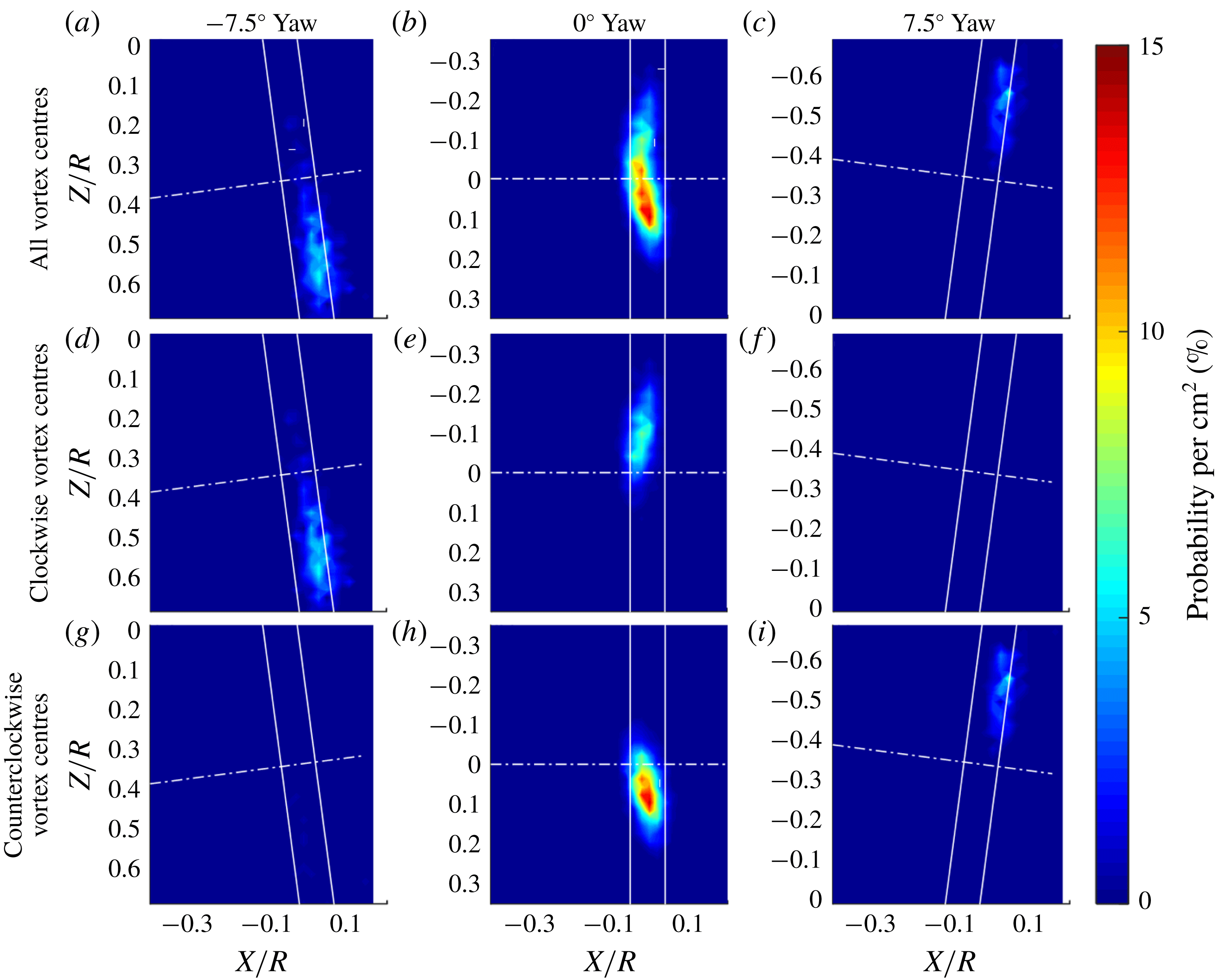
The results of this analysis were captured in terms of probability density functions (PDFs) of vortex centre locations, figure 18. The PDF was obtained for each of the rotor yaw angles by first capturing the locations of all of the vortex centres in all of the velocity measurements at that yaw angle. Then, based on these data, the probability that there would be a vortex within a
 $1~\text{cm}^{2}$
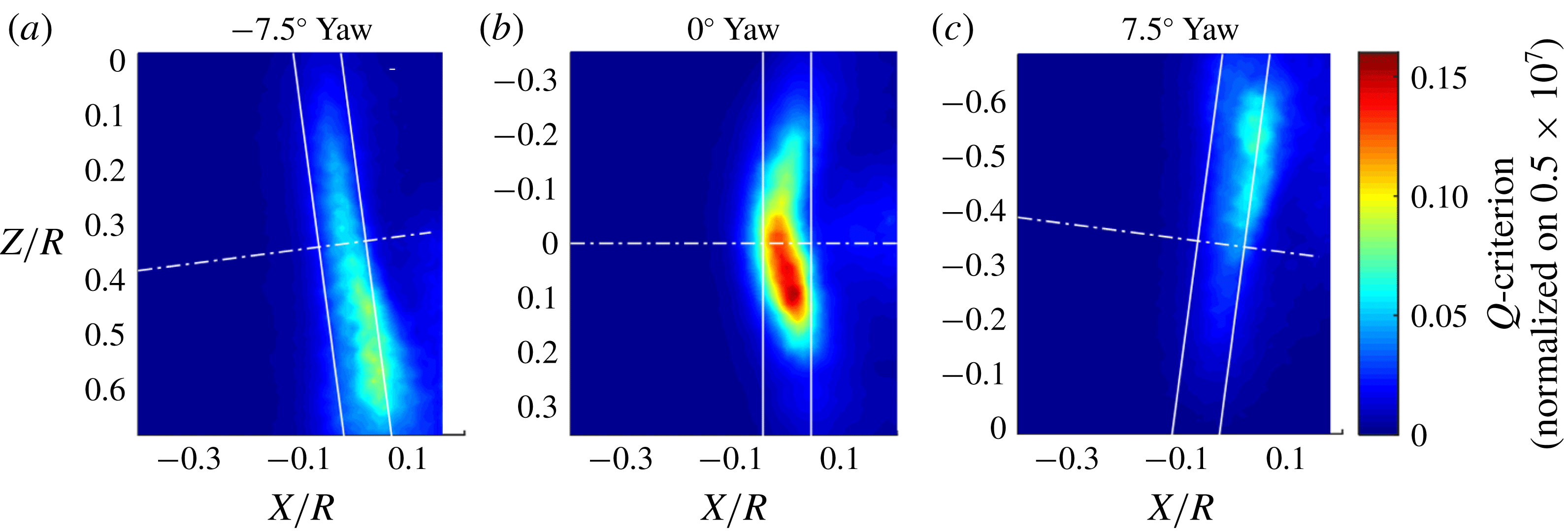
area in any given velocity field measurement was computed at each point in the measurement plane. In each case, the aggregate PDFs are broken down into components showing the locations of counterclockwise (i.e. right-hand rule about the
 $y$
axis) and clockwise rotating structures. Contours of average
 $Q$
-criterion are also shown in figure 19 for the different rotor cases to give a sense of the relative strength of the vortex structures represented in the PDFs. In the unyawed case, the patterns of the contours of average
 $Q$
-criterion (figure 19
b) are very similar to those of the streamwise Reynolds stress, figure 12(b). That is, levels of the highest
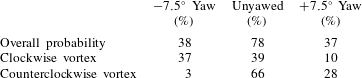
 $Q$
-criteria are in a crescent-shaped region, centred on the separation region beneath the rotor disk but with a marked skew towards the downstroke side. The implication is that not only are turbulence levels highest where the blades are descending into the bottom half of the boundary layer, but the instantaneous flow they are generating is most organized here. The PDF of vortex positions, figure 18(b), also has the crescent form and skew seen in the other plots, showing that coherent vortices are considerably more likely to appear just off of the spanwise centre of the axis of rotation on the downstroke side of the separation region. Figure 18(e,h) shows that the clockwise vortices tend to be found on the upstroke side while the counterclockwise vortices on the downstroke side, consistent with the counter-rotating vortex pair often seen in the instantaneous flow fields for this case, figure 13(e). Counterclockwise vortices are more common, however; the integrated probability of finding a counterclockwise vortex in the tip gap is 66 %, compared with 40 % for a clockwise structure. The bound circulation on the rotor blades as they cut through the boundary layer is also counterclockwise, and thus this bias may indicate that a portion of the structures being observed are blade tip vortices drawn down towards the wall in the region of low-speed flow that surrounds the bottom of the rotor disk. Phase averaged PDFs of vortex position (Murray Reference Murray2016) show that the spatial distribution of vortex centres and the increased likelihood of the counterclockwise vortices was relatively constant through the entire sweep of rotor phase angles. This indicates that the uneven distribution is not caused by an asymmetry associated with the blades approaching the wall versus moving away from the wall.
Probability density functions of the locations of vortices in the tip gap when the rotor is at high thrust (
 $J=0.58$
) and at yaw to the mean inflow. Each point represents the probability of finding a vortex centre in a 1 cm
 $\times$
1 cm area centred on that point in a spatially resolved measurement of the fluid in the tip gap.

The average
 $Q$
-criterion for the yawed and unyawed cases at high thrust (
 $J=0.58$
) shows the relative strengths of the vortex flow structures found in the tip gap across yaw conditions.

Probability density functions of vortex position are shown in figure 18(a,c) for the
 $\pm 7.5^{\circ }$
yawed cases. Contours of average
 $Q$
for the same cases are shown in figure 19(a,c). As noted above, when the rotor is yawed, it is much less likely to exhibit the strong vortex or double vortex structures often seen in the unyawed case, and most instantaneous measurements showed no obvious vortex structures in the tip gap. Consistent with this, the
 $Q$
-criterion analysis found many fewer vortices in the tip gap region when the rotor was yawed, and the contours of average
 $Q$
show peak levels approximately half of those seen with the rotor unyawed. The effects of yaw on the shapes of the PDFs of vortex position (figure 18
a–c) and of the distribution of average
 $Q$
in many ways mirror the effects of yaw on the shape of the time averaged separation region (figure 10
d–f). Vortices are most likely to be found in the elongated region that follows the footprint of the rotor disk on the downstroke side of the rotor for negative yaw (figure 18
a) and the upstroke side for positive yaw (figure 18
c).
Probabilities associated with the PDFs are summarized in table 3; the overall probability is not a sum of clockwise and counterclockwise vortices since multiple vortices can occur simultaneously. However, the probability of observing a coherent vortex structure in the tip gap region at any instant in time considerably reduces with yaw in either direction, from approximately 78 % in the unyawed case to approximately half that at
 $\pm 7.5^{\circ }$
yaw. Although the probability of a vortex appearing in the tip gap is approximately the same at
 $-$
7.5 and
 $+7.5^{\circ }$
yaw, the average
 $Q$
contours clearly show that the vortices are stronger in the
 $-7.5^{\circ }$
case. Almost all of the organized structures formed with the rotor at negative yaw are clockwise rotating vortices, and at positive yaw, counterclockwise vortices are more common by almost three times, figure 18(d–i). This suggests that the prevailing circulation of the mean flow in the plane parallel to the wall (figure 10) is more important in determining the sign of the instantaneous structures than the bound circulation on the blade when the rotor is yawed. This is in sharp contrast to the unyawed case, where both clockwise and counterclockwise vortices are likely to be found in the tip gap. Specifically, there is only a 3 % probability of a counterclockwise vortex occurring at
 $-7.5^{\circ }$
yaw, compared with 66 % at zero yaw and 28 % at
 $+7.5^{\circ }$
yaw. For a clockwise vortex, these probabilities are 37 %, 39 % and 10 % respectively.
Integrated probability of observing a vortex in the tip gap for different yaw angles at the high-thrust condition.
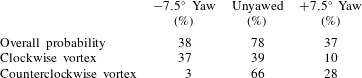
3.4 Coherent vortices as a possible rotor tone noise source
The PIV results above clearly show that the instantaneous near-wall flow under the rotor at low advance ratios is populated by unsteady coherent vortices with axes perpendicular to the wall. Rotor noise in these cases includes quite narrow haystacks, if not tones, at harmonics up to many times the BPF. The question is whether, and how, these observations are connected. In this section, we investigate the hypothesis that this unusual acoustic signature is the result of blade–vortex interaction (BVI), assuming that portions of these vortices are lifted away from the wall in the manner observed by Martio et al. and into the rotor disc, producing sound primarily as a result of two-dimensional parallel BVI. Blade–vortex interactions are well known in helicopter rotor flows (see, for example, Preisser, Brooks & Martin Reference Preisser, Brooks and Martin1994). The specific approach we take here is based on the work of Amiet (Reference Amiet1986).
We consider the case of the unyawed rotor at an advance ratio
 $J$
of 0.58 and, consistent with the mean flow pattern of figure 10(e) and the instantaneous flow of figure 13(e), we consider blades interacting with a pair of counter-rotating vortices. The interaction is idealized as two-dimensional and taking place over a finite portion of the blade span to be defined in terms of the wall-normal (i.e. radial) extent of the vortices. If we assume that the time scale of the vortex movement is large compared with the blade passage time, then the BVIs will result in a periodic time signature and the far-field sound spectrum will have a tonal content with peaks at multiples of the BPF. In the actual flow, we expect that the vortices will move about their mean position, and this will cause some broadening of the peaks around BPFs. The tones will be determined by the broadband spectrum of a single BVI evaluated at multiples of the BPFs
 $\unicode[STIX]{x1D714}=nB\unicode[STIX]{x1D6FA}_{o}$
. Here,
 $B$
is the number of rotor blades,
 $\unicode[STIX]{x1D6FA}_{o}$
is the angular speed of the rotor and
 $n$
is an integer. We consider then two closely spaced vortex interactions. In the present case, the spatial separation of the vortices as seen from an upstream observer position can be considered to be acoustically compact, at least at the two lower harmonics for which the blade chord is less than one quarter of the acoustic wavelength. If
 $\tilde{p}_{BVI}(\boldsymbol{x},\unicode[STIX]{x1D714})$
is the Fourier transform of the acoustic pressure signature at far-field position vector
 $\boldsymbol{x}$
caused by the passage of a single blade past a vortex of strength
 $\unicode[STIX]{x1D6E4}$
with a miss distance
 $h$
, then the repeated interaction of the sequence of rotor blades with a pair of opposite-signed vortices each at the same miss distance gives harmonics with amplitudes
 $$\begin{eqnarray}\displaystyle p_{n}(\boldsymbol{x})=B\unicode[STIX]{x1D6FA}_{o}\tilde{p}_{BVI}(\boldsymbol{x},nB\unicode[STIX]{x1D6FA}_{o})(1-A\text{e}^{\text{i}nB\unicode[STIX]{x1D6FA}_{o}\unicode[STIX]{x1D70F}}). & & \displaystyle\end{eqnarray}$$
Here,
 $\unicode[STIX]{x1D70F}$
is the time taken for the blades to travel between the two vortices and
 $A$
is the ratio of the strength of the second vortex compared with the first. Inspection of the mean PIV results (figure 10
e) suggests that the vortices are on average approximately 0.3
 $R$
apart. Thus,
 $\unicode[STIX]{x1D6FA}_{o}\unicode[STIX]{x1D70F}\approx 0.3$
, and so, for a 10-bladed rotor, one can expect significant phase interference between the individual BVIs at the higher harmonics.
To estimate the far-field sound from a single parallel BVI, we will assume that the vortex core is aligned with the radial direction (parallel to the blade span) when the interaction takes place and make use of a compressible blade response function. For a blade moving with a relative Mach number
 $M$
and an observer at the far-field location
 $x_{1},x_{2},x_{3}$
relative to the blade leading edge at the instant the interaction takes place, the spectrum of the far-field sound is (Glegg & Devenport Reference Glegg and Devenport2017)
 $$\begin{eqnarray}\displaystyle \tilde{p}_{BVI}(\boldsymbol{x},\unicode[STIX]{x1D714})\approx \left(-{\displaystyle \frac{\text{i}\unicode[STIX]{x03C0}\unicode[STIX]{x1D714}x_{2}\text{e}^{\text{i}k_{o}r_{e}-\text{i}k_{o}Mx_{1}}}{c_{\infty }r_{e}^{2}}}\right)\left({\displaystyle \frac{-\text{i}\unicode[STIX]{x1D70C}_{o}c\unicode[STIX]{x1D6E4}L\text{e}^{-\left|\unicode[STIX]{x1D714}h\right|/U_{\infty }}}{4\left(2\unicode[STIX]{x03C0}\right)^{2}}}\right)\unicode[STIX]{x1D6EC}(k_{1}^{(o)},0,\unicode[STIX]{x1D714},M). & & \displaystyle\end{eqnarray}$$
Here,
 $c_{\infty }$
is the speed of sound,
 $r_{e}=\sqrt{x_{1}^{2}+\unicode[STIX]{x1D6FD}^{2}(x_{2}^{2}+x_{3}^{2})}$
is the distance from the source to the observer in Prantl Glauert coordinates,
 $\unicode[STIX]{x1D6FD}=\sqrt{(1-M^{2})}k_{0}$
and
 $k_{1}^{(o)}$
are respectively the scaled acoustic wavenumbers
 $\unicode[STIX]{x1D714}/\unicode[STIX]{x1D6FD}^{2}c_{\infty }$
and
 $k_{o}(x_{1}/r_{e}-M)$
,
 $\unicode[STIX]{x1D70C}_{0}$
is the fluid density,
 $c$
is the blade chord,
 $L$
is the spanwise extent of the BVI and
 $\unicode[STIX]{x1D6EC}$
is the blade response function. In the present problem,
 $M$
is the Mach number corresponding to the tangential velocity
 $U$
of the blade tips as they cut through the separation region. Moreover, the blade relative coordinates
 $x_{1},x_{2},x_{3}$
are respectively in the chordwise, normal to chord and spanwise directions.
Average core vorticity (in
 $\text{s}^{-1}$
) of identified vortices for an unyawed rotor with
 $J=0.58$
.

Even though for the fundamental and first harmonic the blade response function is most accurately given by the incompressible Sears function, the compressible response function performs better over the full frequency range (see Glegg & Devenport Reference Glegg and Devenport2017). For the compressible case,
 $\unicode[STIX]{x1D6EC}$
is inversely proportional to the frequency, and the far-field sound is given as
 $$\begin{eqnarray}\displaystyle \tilde{p}_{BVI}(\boldsymbol{x},\unicode[STIX]{x1D714})\approx \left({\displaystyle \frac{x_{2}\text{e}^{\text{i}k_{o}r_{e}-\text{i}k_{o}Mx_{1}}}{r_{e}^{2}(1-x_{1}/r_{e})^{1/2}}}\right)\left({\displaystyle \frac{\text{i}\unicode[STIX]{x1D70C}_{o}\unicode[STIX]{x1D6E4}L(1-M)^{1/2}M^{1/2}\text{e}^{-|\unicode[STIX]{x1D714}|h/U_{\infty }}}{2(2\unicode[STIX]{x03C0})^{2}}}\right). & & \displaystyle\end{eqnarray}$$
The sound from the vortex-pair interaction will therefore have an overall amplitude that depends on the vortex strength
 $\unicode[STIX]{x1D6E4}$
and a clearly defined spectral shape with a decay rate determined by the miss distance
 $h$
and the strength ratio
 $A$
, and a modulation determined by the vortex spacing
 $U\unicode[STIX]{x1D70F}$
. If the miss distance is small compared with
 $\unicode[STIX]{x1D714}/U$
, then there will be significant high-frequency energy in the spectrum caused by the interaction. Prediction of the sound field requires the circulation of the first interacting vortex
 $\unicode[STIX]{x1D6E4}$
, which was determined using results of the vortex identification analysis of § 3.3. The peak vorticity in each identified structure, averaged over the 11 mm square kernel used in the
 $Q$
-criterion analysis, was recorded and analysed to give the average vortex strength as a function of position (figure 20). The strength is seen to be almost constant, with position at
 $\unicode[STIX]{x1D6E4}=2020~\text{s}^{-1}$
for counterclockwise structures. The value of
 $\unicode[STIX]{x1D6E4}$
was determined by multiplying this value by the kernel area (
 $121~\text{mm}^{2}$
), representing the typical vortex core size, and by the probability of a counterclockwise vortex appearing (66 %, table 3), giving
 $\unicode[STIX]{x1D6E4}=0.16~\text{m}^{2}~\text{s}^{-1}$
. Given its lower probability of appearance (39 %) and average vorticity (
 $-1780~\text{s}^{-1}$
), the second interacting vortex was taken to have a strength of
 $-$
34 %
 $\unicode[STIX]{x1D6E4}$
, i.e.
 $A=0.34$
. The distance between the vortex interactions was taken as the average distance between the vortices,
 $0.3R$
, and so we chose the interaction time delay
 $U\unicode[STIX]{x1D70F}/R=0.3$
. The effective span of the interaction was estimated to be 0.125
 $R$
from the vertical extent of the separation region around the blade tips based on the RANS calculations given in Glegg et al. (Reference Glegg, Buono, Grant, Lachowski, Devenport and Alexander2015). This length includes a doubling to account for the contribution to the sound from reflections in the wall, the blade tip being close enough to the wall for the source and its image to be considered to be acoustically compact at least at the lower harmonics. The vortex miss distance
 $h$
was set to 14 % of the blade chord based on comparison with the acoustic results.
Comparison of the measured spectrum and BVI noise calculation for
 $J=0.58$
in the unyawed rotor: (a) microphone 1; (b) microphone 2.

Calculations of the BVI tones using these parameters are compared with the measured sound spectrum for microphone 1 in figure 21(a). Given the simplicity of the model, the level of agreement is quite surprising. The calculated peak levels are predicted within a dB or two of the measurements for the first seven multiples of the BPF. For microphone 2, located significantly further from the rotor axis at
 $(x,y,z)=$
(
 $-$
2.165, 1.148, 0.225), see figure 1, the estimates are not as close, particularly for the odd-numbered tones. However, the overall levels are still quite realistic, especially considering that these are absolute estimates and given the measurement uncertainty involved with resolving tones when microphone data acquisition is not synchronized with rotor rotation. The calculation is most sensitive to the choice of miss distance. Doubling
 $h$
has little effect on the level of the first tone but changes the shape of the calculated tonal peaks and results in a much more rapid drop-off in the tones as frequency increases than that measured. The difference amounts to some 20 dB by the sixth multiple of the BPF. There is also some sensitivity to the vortex spacing
 $U\unicode[STIX]{x1D70F}$
. Using
 $U\unicode[STIX]{x1D70F}$
of 0.2 rather than 0.3 results in a modulation of the first few tones different from that observed. Nevertheless, the realism of these estimates appears to support the hypothesis that, at low advance ratio, the rotor noise is being generated by BVIs, with the separated flow formed around its blade tips adjacent to the wall.
4 Conclusions
Aeroacoustic measurements and analysis have been made for an unshrouded rotor partially immersed in a planar equilibrium turbulent boundary layer at low Mach number. This configuration provides an idealized model of inflow distortion effects seen when a rotor is mounted adjacent to the hull or fuselage of a vehicle. At low- and moderate-thrust conditions, the rotor produces broadband noise organized into haystacks centred on the BPF and its first few harmonics. These features are produced by large eddies of the ingested turbulence being cut multiple times by successive rotor blades. At high thrust, however, the acoustic signature changes; the haystacks become narrower and start to appear at a much greater range of harmonics. Velocity measurements made in the tip gap show that this change is accompanied by the separation of the boundary layer from the wall in the vicinity of the rotor blade disk. When the rotor axis is aligned with the oncoming flow, an almost symmetric arc-shaped region of reverse flow is formed, bounded by two wall-normal counter-rotating vortex structures. When the rotor is yawed, skewed regions of separation are formed, dominated by secondary flows roughly parallel to the blade disk. In both cases, these regions are highly turbulent and are populated by intense unsteady vortex structures. When the rotor is yawed, the vortex structures tend to be formed with the same sign as the circulation of the mean flow around the separation region. When it is unyawed, and the separation region is most turbulent, the eddies frequently appear as a counter-rotating pair. The assumption that these vortices extend away from the wall into the rotor disk raises the possibility that sound may be produced by a parallel BVI mechanism. Quantitative estimates made on this basis, using the velocity measurements to define the typical vortex strength and spacing, and using the measured sound field to set the miss distance, show tone noise levels consistent with those measured.
Acknowledgements
The authors would like to thank the Office of Naval Research, especially Dr K.-H. Kim and Dr J. Muench, for their support of this research under grants N00014-14-1-0141, N00014-16-1-2395 and N00014-17-1-2698. The assistance of the wind tunnel staff, especially B. Oetjens and T. Meyers, and the AOE Machine Shop during the planning and execution of this test was much appreciated.