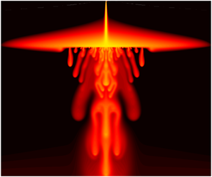


1 Introduction
Buoyancy-driven plumes play a fundamental role in many physical processes across a wide range of scales and environments (Turner Reference Turner1973). In a fluid-saturated porous medium, buoyant plumes form a canonical and generic feature of convective flows (e.g. Hewitt, Neufeld & Lister Reference Hewitt, Neufeld and Lister2012; Slim et al. Reference Slim, Bandi, Miller and Mahadevan2013) and their dynamics plays an important role in geothermal hydrology (Kissling & Weir Reference Kissling and Weir2005), the leakage of dense contaminant from landfill sites (MacFarlane et al. Reference MacFarlane, Cherry, Gillham and Sudicky1983) and the salinization of soil driven by surface evaporation (Wooding et al. Reference Wooding, Tyler, White and Anderson1997; Bauer-Gottwein et al. Reference Bauer-Gottwein, Langer, Prommer, Wolski and Kinzelbach2007). Particular recent interest in the spread of convective plumes is linked to understanding the long-term fate of geologically stored  $\text{CO}_{2}$ (Huppert & Neufeld Reference Huppert and Neufeld2014).
 $\text{CO}_{2}$ injected into subsurface porous formations can dissolve into ambient water within the host rock, increasing its density and driving downwelling convective plumes; the dynamics, spread and interaction of these plumes affects the rate of dissolution of
 $\text{CO}_{2}$, and thus the long-term security of storage.
The theoretical study of buoyancy-driven plumes in a porous medium was pioneered by Wooding (Reference Wooding1963), who derived a similarity solution for an isolated two-dimensional plume by exploiting its long and narrow geometry. Our aim in the present study is to explore the effect on such a plume encountering a thin horizontal layer of a much lower permeability than the surrounding medium. Thin layers of this kind provide a generic form of large-scale heterogeneity in geological media, being a particularly widespread feature of sedimentary formations (Phillips Reference Phillips2009).
A number of authors have considered the role of layers of differing permeability in the context of laterally spreading immiscible gravity currents (Pritchard, Woods & Hogg Reference Pritchard, Woods and Hogg2001; Pritchard & Hogg Reference Pritchard and Hogg2002; Zheng et al. Reference Zheng, Soh, Huppert and Stone2013), while the impact of leakage through discrete fractures or faults on such currents has also been widely studied (Pritchard Reference Pritchard2007; Neufeld et al. Reference Neufeld, Vella, Huppert and Lister2011; Farcas & Woods Reference Farcas and Woods2013; Pegler, Huppert & Neufeld Reference Pegler, Huppert and Neufeld2014). Neufeld & Huppert (Reference Neufeld and Huppert2009) focussed explicitly on the role of a thin, low-permeability horizontal layer on the dynamics of a spreading immiscible gravity current, and derived a simple model for the spread and rise of a buoyant fluid across a series of such layers. An alternative vision of layering, in which the layers are impermeable but contain regular discrete fractures, was studied by Hesse & Woods (Reference Hesse and Woods2010) and Rayward-Smith & Woods (Reference Rayward-Smith and Woods2011), who again described the spread of an immiscible buoyant fluid as it rises through a series of layers, and characterized the effective dispersion induced by the layered structure.
In contrast to these studies of immiscible or laterally spreading fluids, the effect of thin low-permeability or fractured layers on a diffusing plume has not been previously explored. Perhaps the most comparable studies to the present were carried out by Roes, Bolster & Flynn (Reference Roes, Bolster and Flynn2014) and Sahu & Flynn (Reference Sahu and Flynn2017). The former provided a detailed theoretical and experimental study of the dynamics of a descending plume in a porous, confined ‘filling-box’ environment, in which the plume could partially drain through the base of the domain as a rough model of a ‘leaking’ or fractured porous medium. Sahu & Flynn (Reference Sahu and Flynn2017) extended this work to describe the effect of two layers of different permeability in an enclosed domain. These authors showed that, if the lower layer is less permeable, a dense, descending plume can spread laterally as a gravity current over that layer, and drain gradually into it.
The impact of a thin, low-permeability layer on vigorous statistically steady convection in porous media, rather than on an isolated plume, was considered by Hewitt, Neufeld & Lister (Reference Hewitt, Neufeld and Lister2014). They demonstrated that the effect of a thin layer, of thickness ratio  $\unicode[STIX]{x1D700}\ll 1$ (relative to the depth of the host medium) and permeability ratio
 $\unicode[STIX]{x1D6F1}\ll 1$ (relative to that of the host medium), can be parameterized by a single parameter, the impedance
 $\unicode[STIX]{x1D6FA}\sim \unicode[STIX]{x1D700}/\unicode[STIX]{x1D6F1}$ of the layer. They showed that the layer has an increasingly large effect on the convective dynamics and buoyancy flux as
 $\unicode[STIX]{x1D6FA}$ is increased, with the dominant lateral wavelength of the bulk flow increasing significantly with
 $\unicode[STIX]{x1D6FA}$. They also found that a sufficiently large impedance leads to a complete shutdown of advective transport across the layer, so that all the buoyancy is carried across the layer by diffusion. Our main goal in this present work is to investigate and understand the corresponding dynamics for a single plume in the presence of such a layer.
After outlining the model in § 2, we proceed in §§ 3–4 to explore the effect of a thin, horizontal, low-permeability layer on the steady or statistically steady spread of a dense plume falling across the layer. In § 3 we present the results of numerical simulations, and in § 4 we identify and explore the various regimes of spreading at the layer for different values of its impedance  $\unicode[STIX]{x1D6FA}$. We summarize our findings and briefly discuss some physical implications of these results in § 5. Throughout this work we focus on the limit in which the distance to the low-permeability layer is large relative to the distance over which diffusion and advection balance (that is, on the limit of large effective plume Rayleigh number), which is generally the appropriate limit in geophysical settings.
2 Physical model and governing equations
2.1 Dimensional equations
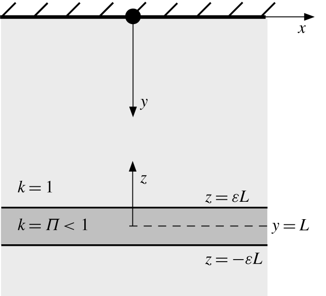
Consider an isolated source of negative buoyancy located at the impermeable rigid upper boundary of a semi-infinite two-dimensional porous medium. The medium is uniform except in a thin, horizontal, low-permeability layer located at some distance below the upper boundary (figure 1). The medium is initially saturated with a fluid of uniform density  $\unicode[STIX]{x1D70C}=\unicode[STIX]{x1D70C}_{0}$, and we assume that the density of fluid containing a concentration
 $c^{\ast }$ of solute is described by a linear equation of state
 $$\begin{eqnarray}\unicode[STIX]{x1D70C}=\unicode[STIX]{x1D70C}_{0}(1+\unicode[STIX]{x1D6FC}c^{\ast }),\end{eqnarray}$$
with  $\unicode[STIX]{x1D6FC}>0$. The buoyancy source, which is assumed to be vanishingly narrow, emits a buoyancy flux
 $B$, which raises the concentration of solute in the medium and so raises the density of the fluid. There is no volume flux from the source and so, under the Boussinesq approximation, the total mass in the system is conserved.
A schematic of the set-up in dimensionless variables. A dense source (black circle) is located on the upper boundary of a semi-infinite two-dimensional porous medium that contains a low-permeability horizontal layer of thickness  $2\unicode[STIX]{x1D700}L\ll L$ and permeability
 $\unicode[STIX]{x1D6F1}\ll 1$, located a distance
 $L$ below the boundary. The equivalent picture in dimensional variables has stars on all the length scales and
 $k^{\ast }=k_{0}^{\ast }k$.

The low-permeability layer is located a distance  $L^{\ast }$ below the source, and has a thickness of
 $2\unicode[STIX]{x1D700}L^{\ast }$, where
 $\unicode[STIX]{x1D700}\ll 1$ is a constant. The medium has uniform permeability
 $k^{\ast }=k_{0}^{\ast }$ except in the low-permeability layer, where
 $k^{\ast }=\unicode[STIX]{x1D6F1}k_{0}^{\ast }$ and
 $\unicode[STIX]{x1D6F1}\ll 1$ is a constant. We assume that the porosity
 $\unicode[STIX]{x1D719}$ is uniform throughout the medium, as would be the case if, for example, the reduction in permeability in the low-permeability layer were due simply to a reduction in mean grain size (see also the discussion in the appendix of Hewitt et al. (Reference Hewitt, Neufeld and Lister2014) about the qualitative effect of a change in porosity in a low-permeability layer).
We introduce a coordinate system ( $x^{\ast },y^{\ast }$) with its origin at the negative buoyancy source, and with the positive
 $y^{\ast }$ direction pointing downwards. For convenience, we also introduce an alternative vertical coordinate
 $z^{\ast }=L^{\ast }-y^{\ast }$, centred on the low-permeability layer (figure 1). The flow
 $\boldsymbol{u}^{\ast }=(u^{\ast },v^{\ast })$ in the medium is incompressible and obeys Darcy’s law, while the concentration evolves over time
 $t^{\ast }$ by advection and diffusion, as described by
 $$\begin{eqnarray}\displaystyle & \displaystyle \unicode[STIX]{x1D735}\boldsymbol{\cdot }\boldsymbol{u}^{\ast }=0, & \displaystyle\end{eqnarray}$$
 $$\begin{eqnarray}\displaystyle & \displaystyle \boldsymbol{u}^{\ast }=-\frac{k^{\ast }}{\unicode[STIX]{x1D707}}(\unicode[STIX]{x1D735}p^{\ast }-\unicode[STIX]{x1D70C}g\boldsymbol{e}_{\boldsymbol{y}}), & \displaystyle\end{eqnarray}$$
 $$\begin{eqnarray}\displaystyle & \displaystyle \unicode[STIX]{x1D719}\frac{\unicode[STIX]{x2202}c^{\ast }}{\unicode[STIX]{x2202}t^{\ast }}+u^{\ast }\frac{\unicode[STIX]{x2202}c^{\ast }}{\unicode[STIX]{x2202}x^{\ast }}+v^{\ast }\frac{\unicode[STIX]{x2202}c^{\ast }}{\unicode[STIX]{x2202}y^{\ast }}=\unicode[STIX]{x1D719}D\unicode[STIX]{x1D6FB}^{2}c^{\ast }, & \displaystyle\end{eqnarray}$$
where  $\boldsymbol{e}_{\boldsymbol{y}}$ is a unit vector in the downwards direction,
 $p^{\ast }$ is the pore pressure,
 $g$ is the gravitational acceleration and
 $\unicode[STIX]{x1D707}$,
 $\unicode[STIX]{x1D719}$ and
 $D$ are the viscosity, porosity and effective diffusivity, respectively, all of which are assumed to be constant. For the purposes of this work, we are interested in steady or statistically steady solutions of these equations.
2.2 Non-dimensional equations
We define the following scales for the concentration, the buoyancy velocity and the length and time scales over which advection and diffusion balance,
 $$\begin{eqnarray}{\hat{c}}=\frac{B}{D},\quad \hat{u} =\frac{\unicode[STIX]{x1D70C}_{0}\unicode[STIX]{x1D6FC}gk_{0}^{\ast }{\hat{c}}}{\unicode[STIX]{x1D707}},\quad \hat{z}=\frac{\unicode[STIX]{x1D719}D}{U},\quad \hat{t}=\frac{\unicode[STIX]{x1D719}\hat{z}}{\hat{u} }=\frac{\unicode[STIX]{x1D719}^{2}D}{\hat{u} ^{2}}.\end{eqnarray}$$
We further introduce dimensionless (unstarred) variables via
 $$\begin{eqnarray}\boldsymbol{u}=\frac{\boldsymbol{u}^{\ast }}{\hat{u} },\quad (x,y,z)=\frac{(x^{\ast },y^{\ast },z^{\ast })}{\hat{z}},\quad c=\frac{c^{\ast }}{{\hat{c}}},\quad k=\frac{k^{\ast }}{k_{0}^{\ast }},\end{eqnarray}$$
 $$\begin{eqnarray}t=\frac{t^{\ast }}{\hat{t}},\quad p=\frac{k_{0}^{\ast }}{\unicode[STIX]{x1D719}D\unicode[STIX]{x1D707}}(p^{\ast }-\unicode[STIX]{x1D70C}_{0}g\hat{z}y),\end{eqnarray}$$
and the dimensionless distance to the low-permeability layer,
 $$\begin{eqnarray}L=\frac{L^{\ast }}{\hat{z}}.\end{eqnarray}$$
After introduction of a streamfunction  $\unicode[STIX]{x1D713}$ with
 $(u,v)=(-\unicode[STIX]{x2202}\unicode[STIX]{x1D713}/\unicode[STIX]{x2202}y,\unicode[STIX]{x2202}\unicode[STIX]{x1D713}/\unicode[STIX]{x2202}x)$, the governing equations (2.2)–(2.4) reduce to
 $$\begin{eqnarray}\displaystyle & \displaystyle \unicode[STIX]{x1D6FB}^{2}\unicode[STIX]{x1D713}=k\frac{\unicode[STIX]{x2202}c}{\unicode[STIX]{x2202}x}, & \displaystyle\end{eqnarray}$$
 $$\begin{eqnarray}\displaystyle & \displaystyle \frac{\unicode[STIX]{x2202}c}{\unicode[STIX]{x2202}t}-\frac{\unicode[STIX]{x2202}\unicode[STIX]{x1D713}}{\unicode[STIX]{x2202}y}\frac{\unicode[STIX]{x2202}c}{\unicode[STIX]{x2202}x}+\frac{\unicode[STIX]{x2202}\unicode[STIX]{x1D713}}{\unicode[STIX]{x2202}x}\frac{\unicode[STIX]{x2202}c}{\unicode[STIX]{x2202}y}=\unicode[STIX]{x1D6FB}^{2}c, & \displaystyle\end{eqnarray}$$
with
 $$\begin{eqnarray}k=\left\{\begin{array}{@{}ll@{}}1\quad & y\leqslant L(1-\unicode[STIX]{x1D700})\\ \unicode[STIX]{x1D6F1}\quad & L(1-\unicode[STIX]{x1D700})<y<L(1+\unicode[STIX]{x1D700})\\ 1\quad & y\geqslant L(1+\unicode[STIX]{x1D700}).\end{array}\right.\end{eqnarray}$$
Since the pressure must remain continuous throughout the medium, the horizontal velocity  $u=-k\unicode[STIX]{x2202}p/\unicode[STIX]{x2202}x$ will be discontinuous at the edges of the low-permeability layer
 $y=L(1\pm \unicode[STIX]{x1D700})$. The buoyancy source imparts a fixed dimensionless buoyancy flux of unity, and so, in a steady state,
 $$\begin{eqnarray}\int _{-\infty }^{\infty }\left(c\frac{\unicode[STIX]{x2202}\unicode[STIX]{x1D713}}{\unicode[STIX]{x2202}x}-\frac{\unicode[STIX]{x2202}c}{\unicode[STIX]{x2202}y}\right)\,\text{d}x=1,\end{eqnarray}$$
at every depth  $y$.
Note that these equations have been scaled in such a way that the dimensionless parameters  $L$,
 $\unicode[STIX]{x1D6F1}$ and
 $\unicode[STIX]{x1D700}$ only appear in the structure of the permeability field (2.11). The distance
 $L$, which is the ratio of the dimensional distance
 $L^{\ast }$ of the layer below the upper boundary to the advection–diffusion length scale
 $\hat{z}$ (2.5c), can also be thought of as an effective Rayleigh number
 $L=L^{\ast }/\hat{z}=\unicode[STIX]{x1D70C}_{0}\unicode[STIX]{x1D6FC}gk_{0}^{\ast }{\hat{c}}L^{\ast }/(\unicode[STIX]{x1D719}D\unicode[STIX]{x1D707})$ for the problem. In geophysical applications,
 $\hat{z}$ is typically of the order of millimetres while
 $L^{\ast }$ might be tens of metres (see § 5), and so we will focus on the limit
 $L\gg 1$.
2.3 The impedance
For the problem of statistically steady convection in the presence of a thin, low-permeability layer, Hewitt et al. (Reference Hewitt, Neufeld and Lister2014) showed that the flow across the layer is driven by the local pressure difference across the layer rather than by buoyancy when  $\unicode[STIX]{x1D700}\ll 1$ and
 $\unicode[STIX]{x1D6F1}\ll 1$. We expect the same behaviour here. In this limit, the vertical component of Darcy’s law (2.3) in the low-permeability layer is
 $$\begin{eqnarray}v=\unicode[STIX]{x1D6F1}\left(\frac{\unicode[STIX]{x2202}p}{\unicode[STIX]{x2202}z}+c\right)=\frac{\unicode[STIX]{x1D6F1}}{2\unicode[STIX]{x1D700}L}\{p|_{z=\unicode[STIX]{x1D700}L}-p|_{z=-\unicode[STIX]{x1D700}L}+O(\unicode[STIX]{x1D700}L)\}.\end{eqnarray}$$
For small  $\unicode[STIX]{x1D700}$ and
 $\unicode[STIX]{x1D6F1}$, (2.13) can be written as a jump condition at
 $z=0$ (
 $y=L$),
 $$\begin{eqnarray}\unicode[STIX]{x1D6FA}v=[p]_{z=0},\quad \;\Longrightarrow \;\quad \unicode[STIX]{x1D6FA}\frac{\unicode[STIX]{x2202}v}{\unicode[STIX]{x2202}x}=-[u]_{z=0},\end{eqnarray}$$
where the square brackets denote the jump in each quantity, and the effective impedance
 $$\begin{eqnarray}\unicode[STIX]{x1D6FA}=\frac{2\unicode[STIX]{x1D700}L}{\unicode[STIX]{x1D6F1}}\end{eqnarray}$$
describes the ratio of the thickness of the layer to its permeability. Recall that  $v$ is the downwards vertical velocity, whereas
 $z$ is measured upwards from the layer.
The problem in the limit  $\unicode[STIX]{x1D700},\unicode[STIX]{x1D6F1}\ll 1$ is thus characterized by two independent parameters,
 $L$ and
 $\unicode[STIX]{x1D6FA}$. We work in this limit for the remainder of this paper. We solved the governing equations (2.9)–(2.10), together with the jump condition (2.14), numerically, as outlined in § A.1. We also carried out a series of computations to confirm the validity of the reduction to the jump condition (2.14), as discussed in § A.2.
3 Phenomenology of numerical solutions
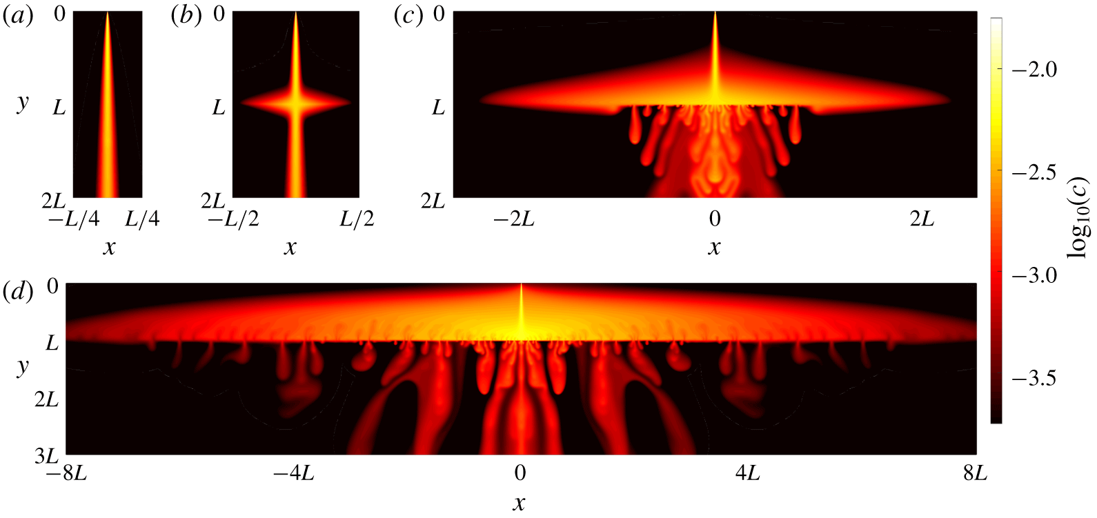
Figure 2 shows a series of steady or statistically steady snapshots from numerical solutions in which the low-permeability layer is parameterized by (2.14) at  $y=L$. For sufficiently low impedance
 $\unicode[STIX]{x1D6FA}$, the layer has a negligible effect on the plume, which simply passes through with no discernible change in its width (figure 2a). For larger values of
 $\unicode[STIX]{x1D6FA}$, the flow across the layer slows down and the pressure difference required to drive flow across the layer forces the plume to spread laterally above the layer (figure 2b). After crossing the layer, the dense fluid below the layer flows back inwards to collect in a single plume again, so that the steady-state flow profile is roughly symmetric above and below the layer. As
 $\unicode[STIX]{x1D6FA}$ is increased further, there are no longer stable steady solutions: while the plume extends further above the low-permeability layer as
 $\unicode[STIX]{x1D6FA}$ increases, the inwards return flow below the layer becomes unstable to a convective boundary-layer-type instability. This instability takes the form of small ‘proto-plumes’ (cf. Hewitt et al. Reference Hewitt, Neufeld and Lister2012) that are continually advected towards the central plume (figure 2c) by the mean return flow. The laterally spreading steady flow above the layer remains stable. For yet larger values of
 $\unicode[STIX]{x1D6FA}$, the flow extends even further over the layer and convective instabilities also appear above the layer (figure 2d). These instabilities also take the form of small proto-plumes, which are advected outwards away from the central plume, in the opposite direction to those below the layer. As described in § 4.5, convection above the layer is driven by the low concentration imposed at the layer by the efficient downwards transport of buoyancy by convection below the layer.
Snapshots of the concentration field, showing  $\log _{10}(c)$ to accentuate the details of the plumes, for an internal layer with
 $L=1.28\times 10^{6}$ and impedance (a)
 $\unicode[STIX]{x1D6FA}=50$, (b)
 $\unicode[STIX]{x1D6FA}=1.02\times 10^{6}$, (c)
 $\unicode[STIX]{x1D6FA}=1.64\times 10^{7}$ and (d)
 $\unicode[STIX]{x1D6FA}=1.05\times 10^{9}$.

In order to characterize the effect of the low-permeability layer on the plume, we define the plume width  $x_{p}$ to be the mean lateral extent over which
 $95\,\%$ of the buoyancy flux is transported across the layer. More precisely, to allow for the possibility of unsteady flow, the instantaneous plume width
 $\tilde{x}_{p}(t)$ at the low-permeability layer is defined implicitly by
 $$\begin{eqnarray}\int _{0}^{\tilde{x}_{p}}\left.\left(cv+\frac{\unicode[STIX]{x2202}c}{\unicode[STIX]{x2202}z}\right)\right|_{z=0}\,\text{d}x=0.95\,\int _{0}^{\infty }\left.\left(cv+\frac{\unicode[STIX]{x2202}c}{\unicode[STIX]{x2202}z}\right)\right|_{z=0}\,\text{d}x,\end{eqnarray}$$
and the mean plume width  $x_{p}$ is the long-time average of
 $\tilde{x}_{p}(t)$.
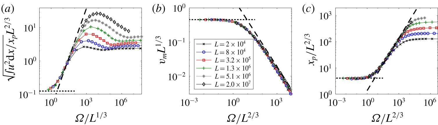
Figure 3 shows data from a series of simulations for different layer depth  $L$ and impedance
 $\unicode[STIX]{x1D6FA}$. For sufficiently low
 $\unicode[STIX]{x1D6FA}$, the velocities and width of the plume at the layer are independent of
 $\unicode[STIX]{x1D6FA}$: the layer has a negligible effect on the plume, which simply passes across it. As
 $\unicode[STIX]{x1D6FA}$ is increased, the horizontal velocity at the layer increases, the vertical velocity across the layer decreases, and the width of the plume increases. For very large
 $\unicode[STIX]{x1D6FA}$, both the horizontal velocity at the layer and the width of the plume appear to become independent of
 $\unicode[STIX]{x1D6FA}$. In the following section, we identify and explore these different regimes of flow.
Scaled data from simulations showing variations with the impedance  $\unicode[STIX]{x1D6FA}$ for different
 $L$ as marked in (b). (a) The root-mean-square horizontal velocity immediately above the low-permeability layer; (b) the maximum vertical velocity
 $v_{m}$ across the low-permeability layer; and (c) the plume width
 $x_{p}$ at the low-permeability layer (3.1). Asymptotic model predictions are shown for a plume with
 $\unicode[STIX]{x1D6FA}=0$ (§ 4.1; short dashed) and for (a) the local perturbation to the plume (§ 4.2) and (b,c) the gravity-current regime (§ 4.3) (long dashed).

4 Asymptotic regimes and theoretical solutions
4.1 Negligible perturbation to the plume: Wooding’s plume solution;  $\unicode[STIX]{x1D6FA}\ll L^{1/3}$

For sufficiently small values of  $\unicode[STIX]{x1D6FA}$, the plume is unaffected at leading order by the impedance of the layer (e.g. figure 2a). In this case, the plume falls and spreads as though in a homogeneous medium and is described by a similarity solution, which was obtained by Wooding (Reference Wooding1963). This solution, which will be useful for our subsequent analysis, is briefly described here.
Sufficiently far below the source, the plume is long and thin so  $x\ll y$ and
 $\unicode[STIX]{x2202}/\unicode[STIX]{x2202}x\gg \unicode[STIX]{x2202}/\unicode[STIX]{x2202}y$. In this limit, Darcy’s law (2.9) implies that the vertical velocity is proportional to the concentration,
 $v=\unicode[STIX]{x2202}\unicode[STIX]{x1D713}/\unicode[STIX]{x2202}x\approx c$, while (2.10) reduces to a balance between advection and horizontal diffusion. Expressing the velocities in terms of the streamfunction we obtain
 $$\begin{eqnarray}-\unicode[STIX]{x1D713}_{y}\unicode[STIX]{x1D713}_{xx}+\unicode[STIX]{x1D713}_{x}\unicode[STIX]{x1D713}_{xy}\approx \unicode[STIX]{x1D713}_{xxx},\end{eqnarray}$$
where subscripts indicate partial derivatives. Equation (4.1) is solved together with conservation of buoyancy flux (2.12), which reduces to  $\int _{-\infty }^{\infty }\unicode[STIX]{x1D713}_{x}^{2}\,\text{d}x=1$ in this limit. These equations permit a similarity solution with
 $$\begin{eqnarray}\unicode[STIX]{x1D713}=\left(\frac{9}{2}\right)^{1/3}y^{1/3}f(\unicode[STIX]{x1D702}),\quad \unicode[STIX]{x1D702}\equiv \frac{x}{48^{1/3}y^{2/3}},\end{eqnarray}$$
and  $f^{\prime \prime \prime }=-2(ff^{\prime \prime }+f^{\prime 2})$,
 $\int _{-\infty }^{\infty }f^{\prime 2}\,\text{d}\unicode[STIX]{x1D702}=4/3$ and
 $f(0)=f^{\prime \prime }(0)=0$. The solution is
 $$\begin{eqnarray}f=\tanh \unicode[STIX]{x1D702},\end{eqnarray}$$
or
 $$\begin{eqnarray}c(x,y)=v(x,y)=6\unicode[STIX]{x1D6FD}^{2}y^{-1/3}\operatorname{sech}^{2}(\unicode[STIX]{x1D6FD}xy^{-2/3}),\end{eqnarray}$$
where  $\unicode[STIX]{x1D6FD}=48^{-1/3}$.
Thus, for a layer located at a depth  $y=L$, the width of the plume
 $x_{p}$ at the layer is
 $x_{p}\sim L^{2/3}$, and the concentration and vertical velocity scale with
 $c\sim v\sim L^{-1/3}$. The plume carries a vertical volume flux
 $vx\sim y^{1/3}$ that increases with depth
 $y$, and entrains fluid from the ambient with a velocity
 $u\sim y^{-2/3}$. Within the plume, the pressure scales with
 $p\sim ux\sim O(1)$.
Given these scalings, the additional condition (2.14) introduced by the low-permeability layer provides a perturbation of order  $\unicode[STIX]{x1D6FA}/L^{1/3}$ to the pressure near the layer. Thus, provided
 $\unicode[STIX]{x1D6FA}\ll L^{1/3}$, the layer has a negligible effect on the spread of the plume (as in figure 2a), and the plume simply passes through the layer. This prediction is corroborated by the collapse of the data in figure 3 for small
 $\unicode[STIX]{x1D6FA}$.
4.2 Local perturbation to plume: $L^{1/3}\ll \unicode[STIX]{x1D6FA}\ll L^{2/3}$

If  $\unicode[STIX]{x1D6FA}\gg O(L^{1/3})$, the pressure jump induced by the low-permeability layer (2.14) is larger than the pressure in the plume, and so the plume solution must break down in the vicinity of
 $y=L$. In order to generate sufficient pressure to drive the plume across the layer, we anticipate that the pressure, and thus the corresponding horizontal velocity, must increase locally in a region near
 $y=L$ of a size comparable to the plume width. We therefore look for a local solution in this region that matches to the similarity solution in § 4.1 sufficiently far above the layer. Motivated by the form of the similarity solution in (4.3)–(4.4), we introduce scaled variables
 $$\begin{eqnarray}P=\frac{p}{\unicode[STIX]{x1D6FD}^{-1}\unicode[STIX]{x1D6FA}L^{-1/3}},\quad U=\frac{u}{\unicode[STIX]{x1D6FA}L^{-1}},\quad (X,Z)=\frac{(x,z)}{\unicode[STIX]{x1D6FD}^{-1}L^{2/3}},\end{eqnarray}$$
and scaled perturbations
 $$\begin{eqnarray}(C,V)=\frac{L}{\unicode[STIX]{x1D6FA}}(c-6\unicode[STIX]{x1D6FD}^{2}L^{1/3}\operatorname{sech}^{2}X,v-6\unicode[STIX]{x1D6FD}^{2}L^{1/3}\operatorname{sech}^{2}X),\end{eqnarray}$$
where  $z=L-y$ and
 $\unicode[STIX]{x1D6FD}=48^{-1/3}$ as previously. The leading-order concentration and vertical velocity
 $6\unicode[STIX]{x1D6FD}^{2}\operatorname{sech}^{2}X$ in (4.6) are simply the unperturbed plume solution from (4.4), but the pressure and horizontal velocity scales in (4.5) are larger than those in the unperturbed plume. Given these scalings, and provided
 $L^{1/3}\ll \unicode[STIX]{x1D6FA}\ll L^{2/3}$, we obtain
 $$\begin{eqnarray}U_{X}-V_{Z}=0,\quad U=-P_{X},\quad V=C+P_{Z},\end{eqnarray}$$
 $$\begin{eqnarray}\displaystyle & \displaystyle 2U\tanh X+C_{Z}=O(L^{1/3}/\unicode[STIX]{x1D6FA},\unicode[STIX]{x1D6FA}/L^{2/3}), & \displaystyle\end{eqnarray}$$
 $$\begin{eqnarray}\displaystyle & \displaystyle [P]_{Z=0}=6\unicode[STIX]{x1D6FD}^{3}\operatorname{sech}^{2}X+O(\unicode[STIX]{x1D6FA}/L^{2/3}), & \displaystyle\end{eqnarray}$$
which imply that the pressure satisfies the elliptic equation
 $$\begin{eqnarray}\unicode[STIX]{x1D6FB}^{2}P=-2\tanh X\frac{\unicode[STIX]{x2202}P}{\unicode[STIX]{x2202}X},\end{eqnarray}$$
to leading order. We expect that  $P\rightarrow 0$ as
 $Z\rightarrow \pm \infty$ so that this local solution matches to the plume above and below the layer. Given the vertical symmetry in (4.10) under
 $Z\rightarrow -Z$ and the jump condition (4.9), we expect the pressure to be antisymmetric about
 $Z=0$, and so the jump condition at
 $Z=0$ (4.9) reduces to a boundary condition
 $P(X,0)=3\unicode[STIX]{x1D6FD}^{3}\operatorname{sech}^{2}X$ for
 $P$ in
 $Z>0$. (Equations (4.7)–(4.9) are invariant under
 $(Z,P,U)\rightarrow -(Z,P,U)$, reflecting the fact that a positive pressure perturbation just above the layer pushes the flow outward a little and a negative perturbation below the layer pulls it back again.)
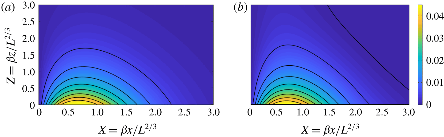
(a) A density map and contours of the predicted horizontal velocity  $U$ above the low-permeability layer from the local-perturbation solution (4.10). (b) Density map and contours of the scaled horizontal velocity
 $L(u-u_{p})/\unicode[STIX]{x1D6FA}$ from a full numerical solution with
 $L=5.12\times 10^{6}$ and
 $\unicode[STIX]{x1D6FA}=2\times 10^{3}$ (for which parameters
 $\unicode[STIX]{x1D6FA}/L^{1/3}\approx 12$ and
 $\unicode[STIX]{x1D6FA}/L^{2/3}\approx 0.07$).

Equation (4.10) can be converted into a Helmholtz equation by a change of variables and solved by a Fourier transform, as outlined in appendix B. The solution takes the form of a local build-up of pressure above the layer, which drives a corresponding horizontal velocity away from the centreline of the plume (figure 4a). Both quantities decay as  $Z\rightarrow \infty$ and the local solution matches to the plume above. Despite the increased horizontal velocity above the low-permeability layer, the vertical velocity across the layer and the width of the plume are both unchanged to leading order by the pressure perturbation. Figure 4(b) shows a scaled density plot of the steady horizontal velocity field from a numerical simulation with parameters lying in this regime, which agrees well with the asymptotic prediction in figure 4(a).
These predictions are also confirmed by the data in figure 3(a), which shows that the horizontal velocity at the layer increases as a function of  $\unicode[STIX]{x1D6FA}/L^{1/3}$, while the vertical velocity and width (figure 3b,c) remain unchanged at that order. For
 $\unicode[STIX]{x1D6FA}\gg L^{2/3}$, the horizontal velocity near the layer becomes sufficiently large to drive significant variations in the concentration and vertical velocity of the plume; in this regime the assumption of a local perturbation breaks down and the width of the plume at the layer increases significantly.
4.3 Gravity current: $\unicode[STIX]{x1D6FA}\gg L^{2/3}$

For  $\unicode[STIX]{x1D6FA}\gg L^{2/3}$, the dense fluid cannot readily cross the low-permeability layer and is diverted sideways away from the main plume to form a gravity current, which has a larger lateral extent than its height (e.g. figure 2b). The extent of this current is such that, in a steady state, there is a balance between the buoyancy flux from the plume, the lateral flow in the current, and the vertical flux across the low-permeability layer.
Within the long, thin, steady current, the pressure is hydrostatic,  $\unicode[STIX]{x2202}p/\unicode[STIX]{x2202}z=-c$, and the lateral flow is given by Darcy’s law,
 $u=-\unicode[STIX]{x2202}p/\unicode[STIX]{x2202}x$. The flow across the low-permeability layer is driven by the pressure difference (2.14) and so
 $p\sim \unicode[STIX]{x1D6FA}v$. Given that
 $(u,v)=(\unicode[STIX]{x2202}\unicode[STIX]{x1D713}/\unicode[STIX]{x2202}z,\unicode[STIX]{x2202}\unicode[STIX]{x1D713}/\unicode[STIX]{x2202}x)$, these balances suggest characteristic horizontal and vertical length scales
 $x\sim \unicode[STIX]{x1D6FA}^{2/3}(\unicode[STIX]{x1D713}/c)^{1/3}$ and
 $z\sim \unicode[STIX]{x1D6FA}^{1/3}(\unicode[STIX]{x1D713}/c)^{2/3}$ for the current. Provided the height of the current near the origin is much less than the depth
 $L$ of the layer, the scales for the streamfunction and concentration are determined by the incoming plume solution at depth
 $L$, for which
 $\unicode[STIX]{x1D713}\sim L^{1/3}$ and
 $c\sim L^{-1/3}$. We thus introduce scaled variables
 $$\begin{eqnarray}X=\frac{x}{\unicode[STIX]{x1D6FD}^{-1/3}\unicode[STIX]{x1D6FA}^{2/3}L^{2/9}},\quad Z=\frac{z}{\unicode[STIX]{x1D6FD}^{-2/3}\unicode[STIX]{x1D6FA}^{1/3}L^{4/9}},\end{eqnarray}$$
 $$\begin{eqnarray}C=\frac{c}{6\unicode[STIX]{x1D6FD}^{2}L^{-1/3}},\quad \unicode[STIX]{x1D6F9}=\frac{\unicode[STIX]{x1D713}}{6\unicode[STIX]{x1D6FD}L^{1/3}},\quad P=\frac{p}{6\unicode[STIX]{x1D6FD}^{4/3}\unicode[STIX]{x1D6FA}^{1/3}L^{1/9}},\end{eqnarray}$$
where  $\unicode[STIX]{x1D6FD}=48^{-1/3}$ as in § 4.1. Given these scalings, it is straightforward to confirm that both the aspect ratio of the current
 $x/z\sim (\unicode[STIX]{x1D6FA}/L^{2/3})^{1/3}$ and the height ratio
 $L/z\sim (\unicode[STIX]{x1D6FA}/L^{5/3})^{-1/3}$ are indeed large provided
 $L^{2/3}\ll \unicode[STIX]{x1D6FA}\ll L^{5/3}$. (We will find below that this upper bound is not achieved owing to the development of convection first below, and then also above, the low-permeability layer.)
The ratio of vertical advection to vertical diffusion in the current, which provides a local Péclet number, also scales with  $Pe\sim (cv)/(c/z)\sim (\unicode[STIX]{x1D6FA}/L^{5/3})^{-1/3}$. Diffusion is therefore negligible in the gravity current as long as
 $\unicode[STIX]{x1D6FA}\ll L^{5/3}$, and buoyancy is transported only by advection along streamlines. Equivalently, the concentration can be written as a function of the streamfunction in the current. Given that in the plume
 $C=\operatorname{sech}^{2}\unicode[STIX]{x1D702}$ and
 $\unicode[STIX]{x1D6F9}=\tanh \unicode[STIX]{x1D702}$ from (4.2) and (4.4), we deduce that
 $$\begin{eqnarray}C=1-\unicode[STIX]{x1D6F9}^{2},\end{eqnarray}$$
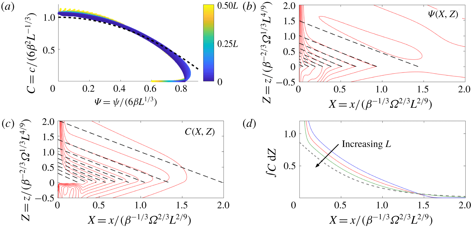
which should hold throughout the current. This relationship  $C(\unicode[STIX]{x1D6F9})$ is verified for a particular numerical solution in figure 5(a).
Within the current, hydrostatic pressure and Darcy’s law can be combined to give
 $$\begin{eqnarray}\frac{\unicode[STIX]{x2202}^{2}P}{\unicode[STIX]{x2202}X\unicode[STIX]{x2202}Z}=-\frac{\unicode[STIX]{x2202}C}{\unicode[STIX]{x2202}X}=-\frac{\unicode[STIX]{x2202}^{2}\unicode[STIX]{x1D6F9}}{\unicode[STIX]{x2202}Z^{2}},\end{eqnarray}$$
or, given (4.13),
 $$\begin{eqnarray}\frac{\unicode[STIX]{x2202}\unicode[STIX]{x1D6F9}}{\unicode[STIX]{x2202}X}=-\frac{1}{2\unicode[STIX]{x1D6F9}}\frac{\unicode[STIX]{x2202}^{2}\unicode[STIX]{x1D6F9}}{\unicode[STIX]{x2202}Z^{2}}.\end{eqnarray}$$
Numerical solutions for moderate  $\unicode[STIX]{x1D6FA}$ show a roughly symmetric concentration profile above and below the low-permeability layer (e.g. figure 2b). Motivated by this observation, and by the vertical symmetry in (4.15) under
 $Z\rightarrow -Z$, we look for solutions for which the streamfunction is symmetric and the pressure antisymmetric across the layer. Under this assumption
 $[p]_{z=0}=2p(x,0)$ and (2.14) reduces to
 $$\begin{eqnarray}\left.\frac{\unicode[STIX]{x2202}\unicode[STIX]{x1D6F9}}{\unicode[STIX]{x2202}X}\right|_{Z=0}=2\int _{0}^{\infty }1-\unicode[STIX]{x1D6F9}^{2}\,\text{d}Z.\end{eqnarray}$$
Away from the current, the flow matches to a uniform far field with  $C=0$, and thus
 $\unicode[STIX]{x1D6F9}\rightarrow 1$ as
 $(X,Z)\rightarrow \infty$. On the scale of the current, the plume appears as a source on the line
 $X=0$, with the limiting values of
 $\unicode[STIX]{x1D6F9}(0,Z)$ giving the flux from the plume and with
 $\unicode[STIX]{x1D6F9}(0,0)=0$. The profile
 $\unicode[STIX]{x1D6F9}(0,Z)$ is not prescribed, but is determined as part of the solution by the ‘downstream’ drainage flow in the current.
(a–c) Comparison of the gravity-current model with simulations for  $L=1.28\times 10^{6}$ and
 $\unicode[STIX]{x1D6FA}=4.1\times 10^{6}$ (
 $\unicode[STIX]{x1D6FA}/L^{2/3}=348$). (a) A scatter plot of
 $c(x,z)$ against
 $\unicode[STIX]{x1D713}(x,z)$ for all numerical grid cells in the range
 $0\leqslant z<L/2$, together with the prediction (4.13) for the gravity current (dashed line). Points are coloured by their
 $z$ value. (b,c) Equally spaced contours (red solid) of (b) the time-averaged streamfunction
 $\unicode[STIX]{x1D6F9}(X,Z)$ and (c) the time-averaged concentration
 $C(X,Z)$ together with the predictions of the gravity-current model (black dashed). (d) The vertically integrated concentration in the current, for simulations with a fixed ratio
 $\unicode[STIX]{x1D6FA}/L=3.2$ and with
 $L=3.2\times 10^{5}$ (blue),
 $L=1.28\times 10^{6}$ (red) and
 $L=5.12\times 10^{6}$ (green), together with the prediction of the gravity-current model (dashed).

We solve the nonlinear diffusion equation (4.15) numerically by integrating in from  $X\gg 1$, using the linearized equation in the limit
 $X\rightarrow \infty$ as an ‘initial’ condition. In this limit, we expect
 $\unicode[STIX]{x1D6F9}\rightarrow 1$, and so
 $\unicode[STIX]{x1D6F7}\equiv 1-\unicode[STIX]{x1D6F9}\ll 1$ satisfies the linear diffusion problem
 $$\begin{eqnarray}-\frac{\unicode[STIX]{x2202}\unicode[STIX]{x1D6F7}}{\unicode[STIX]{x2202}X}=\frac{1}{2}\frac{\unicode[STIX]{x2202}^{2}\unicode[STIX]{x1D6F7}}{\unicode[STIX]{x2202}Z^{2}},\quad -\left.\frac{\unicode[STIX]{x2202}\unicode[STIX]{x1D6F7}}{\unicode[STIX]{x2202}X}\right|_{Z=0}=4\int _{0}^{\infty }\unicode[STIX]{x1D6F7}\,\text{d}Z.\end{eqnarray}$$
Solution of the linear problem gives
 $$\begin{eqnarray}\unicode[STIX]{x1D6F9}(X\rightarrow \infty )\sim 1-\unicode[STIX]{x1D706}\text{e}^{-2X-2Z},\quad C(X\rightarrow \infty )\sim 2\unicode[STIX]{x1D706}\text{e}^{-2X-2Z},\end{eqnarray}$$
where the constant  $\unicode[STIX]{x1D706}$, and the full nonlinear solution, are determined by matching to (4.15) and integrating inwards numerically to
 $\unicode[STIX]{x1D6F9}(0,0)=0$. This yields
 $\unicode[STIX]{x1D706}\approx 1.14$.
Both the predicted scalings of the model and the quantitative predictions of the plume width and vertical velocity across the layer give good agreement with full numerical simulations, as shown in figure 3(b,c). In particular, we can extract the width of the current  $x_{p}$ at the layer from the full nonlinear solution of the model and combine with the scalings in (4.11a) to find that
 $$\begin{eqnarray}x_{p}\approx 1.37\unicode[STIX]{x1D6FA}^{2/3}L^{2/9}\end{eqnarray}$$
(long-dashed line in figure 3c). Further comparison between the model and numerical simulations is presented in figure 5. Figure 5(b,c) show streamlines and contours of the concentration near the low-permeability layer for a particular numerical simulation, each of which take the form of almost straight diagonal lines through the gravity current. The model predictions, given by the full nonlinear solution of (4.15), provide reasonable agreement, particularly for the streamlines (figure 5b). Profiles of the vertically integrated concentration through the current (figure 5d) show that the numerical solutions increasingly approach the prediction of the model as the ratio  $\unicode[STIX]{x1D6FA}/L^{2/3}$ is increased.
The main discrepancy between the model and simulations can be seen in the concentration contours of figure 5(c): the concentration at the base of the plume is higher than the model predicts. This difference occurs because the balance between vertical advection and horizontal diffusion in the plume breaks down as the buoyancy starts to spread laterally into the gravity current; horizontal diffusion weakens, and so the concentration down the centreline decreases more slowly with depth than in the ideal plume solution.
Diffusion also affects the current along its base, where the contours bend around before crossing the low-permeability layer (figure 5c), smoothing out the sharp jump in concentration gradient that is predicted by the model. The resultant boundary layer just above the low-permeability layer has a depth  $\unicode[STIX]{x1D6FF}$ given by a balance between vertical diffusion and downwards advection,
 $\unicode[STIX]{x1D6FF}\sim 1/v\sim \unicode[STIX]{x1D6FA}^{2/3}L^{-1/9}$. A simple boundary-layer analysis in the vicinity of the low-permeability layer indicates that the contribution to the buoyancy flux across the layer from diffusion is a factor of
 $1/Pe=(\unicode[STIX]{x1D6FA}/L^{5/3})^{1/3}$ smaller than the
 $O(1)$ advective flux. However, we will find below that convection both below the low-permeability layer and, for larger
 $\unicode[STIX]{x1D6FA}$, above the layer, causes an increase in the diffusive flux across it. In particular, convection above the layer provides a mechanism to mix up the gravity current and change the structure of the flow above the layer. We will return to discuss the scalings associated with the development of convection below and above the layer in § 4.5, after first describing the flow above the low-permeability layer in the regime for which
 $\unicode[STIX]{x1D6FA}$ is sufficiently large that convection is well established and advection across the layer is negligible.
4.4 Large-scale circulation: ‘ultimate’ regime with $\unicode[STIX]{x1D6FA}\gg L$

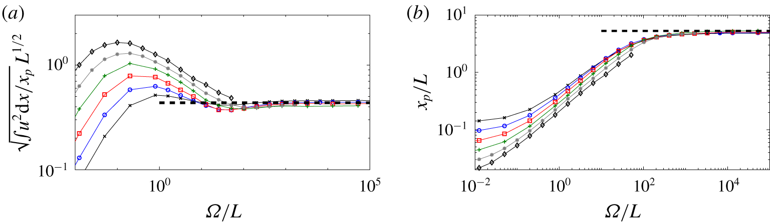
For sufficiently large values of the impedance  $\unicode[STIX]{x1D6FA}$, we expect that the advective transport across the low-permeability layer is negligible and so the flow above the layer must recirculate with a negligible volume flux across the layer. Given this, we also expect that the flow above the layer becomes independent of
 $\unicode[STIX]{x1D6FA}$. Data from simulations (figure 3a,c) confirm this prediction as
 $\unicode[STIX]{x1D6FA}\rightarrow \infty$. Snapshots of the flow in this limit (e.g. figure 2d) further suggest that the spread of the plume above the low-permeability layer is strongly affected by convective instabilities, which penetrate an appreciable distance up from the layer.
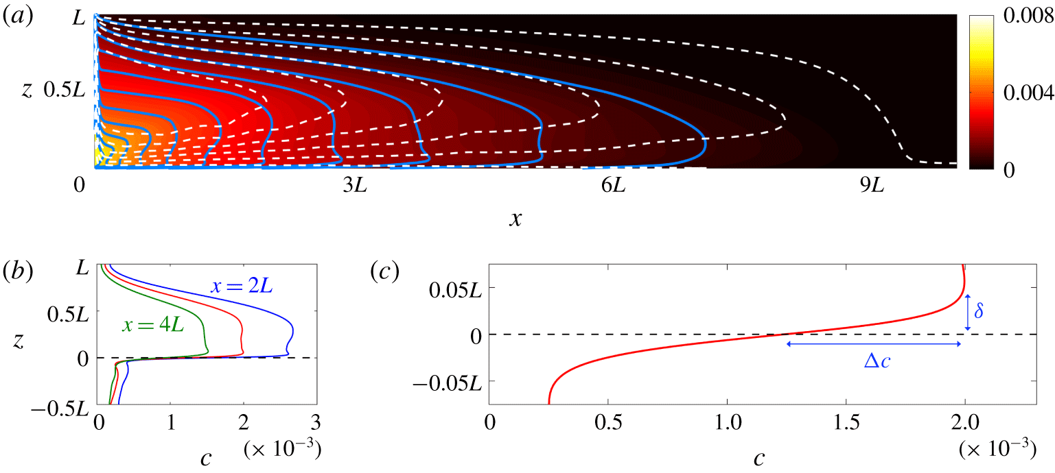
(a) Time-averaged colour map of the concentration above the low-permeability layer when the impedance  $\unicode[STIX]{x1D6FA}$ is large (
 $L=1.28\times 10^{6}$ and
 $\unicode[STIX]{x1D6FA}=1.05\times 10^{9}$, as in figure 2d), overlain by contours of the time-averaged concentration (blue solid) and time-averaged streamlines (white dashed). (b) Vertical profiles of the time-averaged concentration at
 $x=2L$,
 $x=3L$ and
 $x=4L$ from the same computation. (c) An enlarged plot of the same data at
 $x=3L$, showing the structure of the concentration field near the low-permeability layer.

A time-averaged plot of the concentration and streamlines (figure 6a) reveals more clearly the nature of the flow for very large  $\unicode[STIX]{x1D6FA}$. The lateral flow fills the depth
 $0<z<L$, with roughly the lower half flowing away from the central downwelling plume at
 $x=0$ and the upper half being a return flow back towards the plume. The concentration in the outflowing lower half varies only weakly with depth (figure 6b), illustrating that it is well mixed by convection. In the return flow, by contrast, the concentration contours align roughly with the streamlines (figure 6a), indicating that there is very little mixing in this region.
Motivated by these observations, we consider a model in which a long, thin gravity current of depth  $h(x)$ flows away from the central plume and is vertically well mixed with a time-averaged concentration
 $\overline{c}(x)$. The current loses buoyancy across the very low permeability layer at its base by diffusion through a narrow boundary layer of depth
 $\unicode[STIX]{x1D6FF}\ll h$ and concentration drop
 $\unicode[STIX]{x0394}c$ (figure 6c). Below the layer, buoyancy diffuses through another boundary layer and is transported rapidly away from the layer by convection. With vigorous convection both above and below the layer, we expect that
 $\unicode[STIX]{x0394}c\sim \overline{c}/2$, and so the diffusive flux across the layer scales with
 $\unicode[STIX]{x0394}c/\unicode[STIX]{x1D6FF}\sim \overline{c}/\unicode[STIX]{x1D6FF}$. The impedance
 $\unicode[STIX]{x1D6FA}$ plays no role in this construction, since the advective transport across the low-permeability layer is negligible if
 $\unicode[STIX]{x1D6FA}$ is sufficiently large.
Following classical arguments for convection (e.g. Howard Reference Howard and Görtler1964), we assume that the boundary layer just above the low-permeability layer is maintained at a marginally stable depth: any growth of the boundary layer beyond this marginal depth is rapidly transported away by high-wavenumber convective instabilities. Equivalently, the local boundary-layer Rayleigh number  ${\sim}\unicode[STIX]{x0394}c\,\unicode[STIX]{x1D6FF}\sim \overline{c}\unicode[STIX]{x1D6FF}$ is maintained at a critical value
 $\overline{c}\unicode[STIX]{x1D6FF}\sim R_{c}$. The diffusive flux across the layer therefore scales with
 ${\sim}\unicode[STIX]{x0394}c/\unicode[STIX]{x1D6FF}\sim \overline{c}/\unicode[STIX]{x1D6FF}\sim \overline{c}^{2}/R_{c}$. For notational convenience, we set the flux to be equal to
 $\overline{c}^{2}/R_{c}$ by suitably absorbing any
 $O(1)$ constants of proportionality into our definition of
 $R_{c}$. Comparison with previous studies of porous convection (e.g. Hewitt, Neufeld & Lister Reference Hewitt, Neufeld and Lister2013; Slim Reference Slim2014) suggests that
 $R_{c}=O(10^{2})$.
In both the outflowing and returning currents in  $0<z<L$, we expect that the pressure is hydrostatic and the horizontal velocity is driven by Darcy’s law,
 $u\sim \unicode[STIX]{x1D713}/z\sim cz/x$. A balance of the lateral buoyancy flux through the current with that diffusing across the low-permeability layer indicates that
 $ucz\sim xc^{2}/R_{c}\sim 1$. Given these scalings, together with the observation that the flow fills the depth
 $L$, we introduce scaled variables
 $$\begin{eqnarray}(Z,H)=\frac{(z,h)}{L},\quad X=\frac{x}{R_{c}^{1/2}L},\quad C=\frac{\langle c\rangle }{R_{c}^{1/4}L^{-1/2}},\quad P=\frac{\langle p\rangle }{R_{c}^{1/4}L^{1/2}},\end{eqnarray}$$
 $$\begin{eqnarray}\unicode[STIX]{x1D6F9}=\frac{\langle \unicode[STIX]{x1D713}\rangle }{R_{c}^{-1/4}L^{1/2}},\quad U=\frac{\langle u\rangle }{R_{c}^{-1/4}L^{-1/2}},\quad V=\frac{\langle v\rangle }{R_{c}^{-3/4}L^{-1/2}},\end{eqnarray}$$
where the angle brackets  $\langle \cdot \rangle$ signify the long-time average. Note that the horizontal and vertical scales of the flow both scale with the layer depth
 $L$, but differ by a factor of the (moderately large) parameter
 $R_{c}^{1/2}$, so the flow remains appreciably longer than it is deep. Note also that the concentration scale
 $R_{c}^{1/4}L^{-1/2}$ is weaker than the scale
 $L^{-1/3}$ in the plume, which is a consequence of convective mixing of low-concentration fluid at the low-permeability layer into the flow above, as will be discussed again in § 4.5.
We define the height of the current  $Z=H(X)$ to be the contour that separates the outflow below from the return flow above, so
 $U(Z=H)=0$. In the out-flowing region
 $Z<H$, the concentration
 $C(X,Z)=\overline{C}(X)$ is well mixed by convection, and hydrostatic pressure and Darcy’s law combine to give
 $$\begin{eqnarray}\frac{\unicode[STIX]{x2202}U}{\unicode[STIX]{x2202}Z}=-\frac{\unicode[STIX]{x2202}^{2}P}{\unicode[STIX]{x2202}X\unicode[STIX]{x2202}Z}=\frac{\unicode[STIX]{x2202}\overline{C}}{\unicode[STIX]{x2202}X}\end{eqnarray}$$
or
 $$\begin{eqnarray}U=-\frac{\unicode[STIX]{x2202}\overline{C}}{\unicode[STIX]{x2202}X}(H-Z).\end{eqnarray}$$
Vertical integration of (4.23) yields an outward volume flux  $-H^{2}\overline{C}_{X}/2$.
Buoyancy in the current is advected laterally away from the central downwelling plume and is lost both by diffusion across the low-permeability layer at the base of the current and by advection across  $Z=H$, where it is entrained into the return flow in
 $H<Z<L$. This flux balance is represented in the vertically integrated advection–diffusion equation (2.10),
 $$\begin{eqnarray}\frac{\unicode[STIX]{x2202}}{\unicode[STIX]{x2202}X}\left(\frac{\overline{C}H^{2}}{2}\frac{\unicode[STIX]{x2202}\overline{C}}{\unicode[STIX]{x2202}X}\right)=\overline{C}^{2}+V|_{Z=H}\overline{C},\end{eqnarray}$$
where the vertical velocity at  $Z=H(X)$ is given by the vertically integrated equation of volume conservation (2.2),
 $V|_{Z=H}=(H^{2}\overline{C}_{X}/2)_{X}$. Equation (4.24) thus reduces to
 $$\begin{eqnarray}\frac{H^{2}}{2}\left(\frac{\unicode[STIX]{x2202}\overline{C}}{\unicode[STIX]{x2202}X}\right)^{2}=\overline{C}^{2}\quad \;\Longrightarrow \;\quad \frac{\unicode[STIX]{x2202}\overline{C}}{\unicode[STIX]{x2202}X}=-\sqrt{2}\frac{\overline{C}}{H},\end{eqnarray}$$
with solution
 $$\begin{eqnarray}\overline{C}(X)=C_{0}\exp \left[-\sqrt{2}\int _{0}^{X}H^{-1}\,\text{d}X\right],\end{eqnarray}$$
where the constant  $C_{0}$ is determined by the constraint of unit total buoyancy flux across the low-permeability layer,
 $\int _{-\infty }^{\infty }\overline{C}^{2}\,\text{d}X=2\int _{0}^{\infty }\overline{C}^{2}\,\text{d}X=1$. We can also integrate
 $U=\unicode[STIX]{x1D6F9}_{Z}$ (4.23) using (4.25) to obtain the corresponding streamfunction
 $$\begin{eqnarray}\unicode[STIX]{x1D6F9}(X,Z)=\frac{H\overline{C}(X)}{\sqrt{2}}\left[\frac{2Z}{H}-\left(\frac{Z}{H}\right)^{2}\right].\end{eqnarray}$$
In particular, streamlines carry fluid across the boundary  $Z=H$ and enter into the return flow in
 $Z>H$ with
 $$\begin{eqnarray}\unicode[STIX]{x1D6F9}(X,H(X))=\frac{H(X)\overline{C}(X)}{\sqrt{2}}.\end{eqnarray}$$
In the return flow ( $Z>H$), we assume that diffusion is negligible and that convective mixing does not penetrate from
 $Z<H$. Concentration is thus advected from the boundary
 $Z=H(X)$ along streamlines, and
 $C(X,Z)=C(\unicode[STIX]{x1D6F9})$, where
 $C(\unicode[STIX]{x1D6F9})$ is given by (4.28). Once again, hydrostatic pressure and Darcy’s law combine to give
 $$\begin{eqnarray}\frac{\unicode[STIX]{x2202}^{2}\unicode[STIX]{x1D6F9}}{\unicode[STIX]{x2202}Z^{2}}=\frac{\unicode[STIX]{x2202}C}{\unicode[STIX]{x2202}X},\end{eqnarray}$$
in  $Z>H$, with three boundary conditions
 $$\begin{eqnarray}\unicode[STIX]{x1D6F9}(Z=1)=0,\quad \unicode[STIX]{x1D6F9}_{Z}(Z=H)=0,\quad C(Z=H)=\overline{C},\end{eqnarray}$$
which are sufficient both to solve (4.29) and to determine the unknown contour  $Z=H(X)$. In fact, (4.29)–(4.30) have a separable solution with
 $H$ independent of
 $X$, given by
 $$\begin{eqnarray}C(X,Z)=\frac{\sqrt{2}}{H}\unicode[STIX]{x1D6F9}(X,Z)=\overline{C}(X)\sin \left[\frac{\sqrt{2}\left(1-Z\right)}{H}\right],\end{eqnarray}$$
where
 $$\begin{eqnarray}H=\frac{2\sqrt{2}}{2\sqrt{2}+\unicode[STIX]{x03C0}}\approx 0.47.\end{eqnarray}$$
The division between well-mixed lower fluid and returning fluid is thus independent of the distance from the central plume, and lies marginally below half way between the upper boundary and the low-permeability layer.
Given that  $H$ is a constant, we deduce that
 $C_{0}^{2}=\sqrt{2}/H$ in (4.26), and thus that the solution throughout the domain is
 $$\begin{eqnarray}C=\overline{C}(X){\hat{C}}(Z),\quad \unicode[STIX]{x1D6F9}=\frac{H}{\sqrt{2}}\overline{C}(X)\hat{\unicode[STIX]{x1D6F9}}(Z),\quad \overline{C}(X)=\frac{2^{1/4}}{H^{1/2}}\exp \left[-\frac{\sqrt{2}X}{H}\right],\end{eqnarray}$$
where
 $$\begin{eqnarray}\left.\begin{array}{@{}ll@{}}{\hat{C}}=\hat{\unicode[STIX]{x1D6F9}}=\sin [\sqrt{2}(1-Z)/H] & \text{in }Z>H,\\ {\hat{C}}=1,\hat{\unicode[STIX]{x1D6F9}}=2Z/H-(Z/H)^{2} & \text{in }Z<H,\end{array}\right\}\end{eqnarray}$$
and  $H$ is given by (4.32). We thus have a complete analytical solution for the ultimate regime in which the flow is well mixed by convection in
 $Z<H$ and there is only diffusive transport across the low-permeability layer at
 $Z=0$.
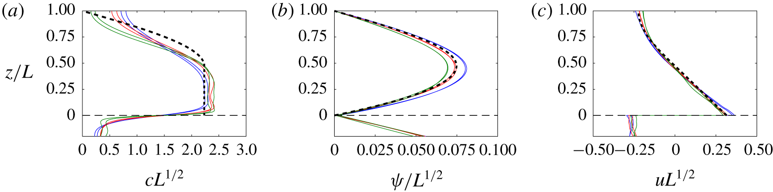
Time-averaged vertical profiles at  $x=3L$ of (a) the concentration
 $c$, (b) the streamfunction
 $\unicode[STIX]{x1D713}$ and (c) the horizontal velocity
 $u$ from simulations with
 $L=[8,32,128]\times 10^{4}$ (blue, red, green) and
 $\unicode[STIX]{x1D6FA}=[32,128]\times 100L$ in each case. Model predictions from (4.33) with
 $R_{c}=100$ are overlaid (dashed black).

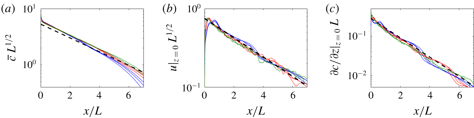
Time-averaged horizontal profiles of (a) the vertically averaged concentration  $\overline{c}(x)=(1/h)\int _{0}^{h}c\,\text{d}z$ with
 $h=HL$ given by (4.32), (b) the horizontal velocity
 $u(x,0)$ and (c) the flux
 $\unicode[STIX]{x2202}c/\unicode[STIX]{x2202}z$ across the layer from simulations with
 $L=[8,32,128]\times 10^{4}$ (blue, red, green) and
 $\unicode[STIX]{x1D6FA}=[8,32,128]\times 100L$ in each case. Model predictions from (4.33) with
 $R_{c}=100$ are overlaid (dashed black).

The critical Rayleigh number  $R_{c}=O(10^{2})$, which appears in the rescalings in (4.20) and (4.21), is a free parameter in this model. Comparison of the diffusive flux across the layer with
 $\overline{c}^{2}$ from numerical simulations yields a value of
 $R_{c}\approx 100$, which we use in our comparisons here. Time-averaged data showing both the vertical structure of the flow (figure 7) and the horizontal structure of the flow for
 $Z<H$ (figure 8) for sufficiently large
 $\unicode[STIX]{x1D6FA}$ show a good collapse with the predicted scalings and a very reasonable quantitative agreement with the model predictions. The largest errors in the model appear in the concentration profiles for
 $Z>H$ (figure 7a), and comparison with the corresponding streamfunction (figure 7b) suggests that there is a slight deviation from the relationship
 $C(\unicode[STIX]{x1D6F9})$ (4.31) in
 $Z>H$. We attribute this deviation partly to the boundary condition
 $\unicode[STIX]{x2202}c/\unicode[STIX]{x2202}z=0$ at the upper boundary in the simulations, and partly to residual convective motion crossing
 $Z=H$ and driving cross-streamline mixing.
The corrections to this model associated with a finite impedance  $\unicode[STIX]{x1D6FA}$ come from the weak advective flux
 $F_{a}$ across the low-permeability layer, given by
 $F_{a}=-\int cv\,\text{d}x\sim cpx/\unicode[STIX]{x1D6FA}\sim R_{c}L/\unicode[STIX]{x1D6FA}$. This flux is negligible for
 $\unicode[STIX]{x1D6FA}\gg R_{c}L$, which we thus identify as the range of the ultimate regime. The scaling
 $\unicode[STIX]{x1D6FA}\sim R_{c}L$ for the onset of this regime is corroborated by the collapse of the horizontal velocity at the layer and the plume width in figure 9(a,b). The same data also show good quantitative agreement with the model predictions for
 $\unicode[STIX]{x1D6FA}\gg L$. In particular, the width of the current at the layer is
 $$\begin{eqnarray}x_{p}\approx 5.3L.\end{eqnarray}$$
We note, in ending the discussion of this regime, that the central plume does not explicitly enter the model construction outlined here. The numerical simulations suggest that the basic structure of the original plume continues to survive near  $x=0$, with a width
 $x\sim L^{2/3}$ that is much less than the width of the main current and a concentration scale
 $c\sim L^{-1/3}$ that is greater than that of the main flow. However, unlike in the gravity-current regime, the plume scales do not control the dynamics in the main circulating flow in this regime. Some remnant evidence of the central plume can be discerned near
 $x=0$ in the concentration and horizontal-velocity profiles in figure 8(a,b).
(a) The root-mean-square horizontal velocity immediately above the low-permeability layer and (b) the plume width  $x_{p}$, showing the same raw data as in figure 3(a,c), respectively, but scaled to show the collapse in the ultimate regime. Dashed lines show the predictions of the model in the ultimate regime.

4.5 Transitional regime: $R_{c}^{3/2}L^{2/3}\ll \unicode[STIX]{x1D6FA}\ll R_{c}L$

If the flow near the layer remained steady, we would expect the gravity-current regime discussed in § 4.3 to apply until diffusion becomes important at  $\unicode[STIX]{x1D6FA}\sim L^{5/3}$. However, the flow does not remain steady as
 $\unicode[STIX]{x1D6FA}$ is increased, and, as discussed in § 4.4, for
 $\unicode[STIX]{x1D6FA}\gg R_{c}L$ the flow is in the ‘ultimate’ regime in which vigorous convection mixes up fluid above the low-permeability layer. Furthermore, the gravity-current regime cannot simply match smoothly to the ultimate regime when
 $\unicode[STIX]{x1D6FA}\sim R_{c}L$, because the scalings (in (4.11) and (4.20), respectively) do not match smoothly. For example, at
 $\unicode[STIX]{x1D6FA}\sim R_{c}L$ the width of the current predicted by the gravity-current regime in (4.19) is too narrow (
 $x_{p}\sim R_{c}^{2/3}L^{8/9}$) relative to that in the ultimate regime (
 $x_{p}\sim R_{c}^{1/2}L$), while the concentration scale is too large (
 $c\sim L^{-1/3}$ relative to
 $c\sim R_{c}^{1/4}L^{-1/2}$).
A different flow regime must, therefore, fill the gap between the gravity-current regime and the ultimate regime. Relative to the gravity-current regime, the key difference in this transitional regime is the presence of convective instabilities above the layer which mix up the fluid. Relative to the ultimate regime, the key difference is that there is a significant loss of buoyancy by advection across the low-permeability layer, rather than all of the fluid circulating above the layer without leaking across it.
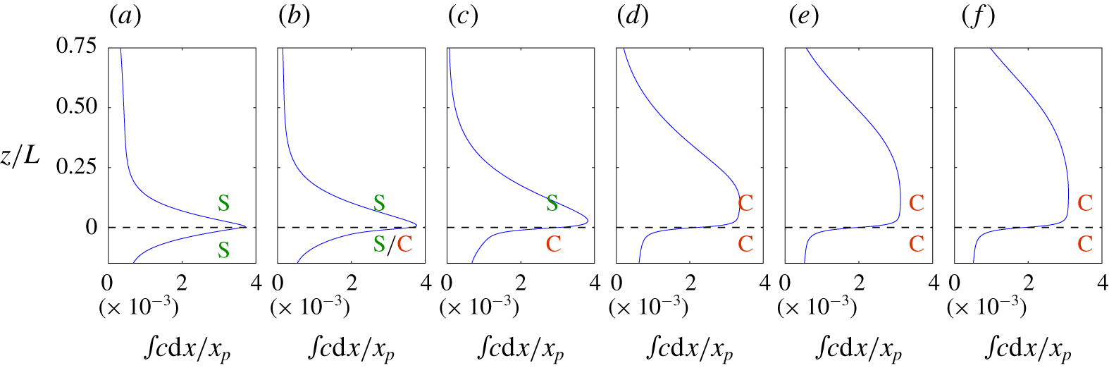
In this section we briefly outline the scaling balances of the transitional regime, beginning with a discussion of convection below the low-permeability layer. To help frame the discussion, figure 10 shows plots of the horizontally integrated concentration across the layer from a series of computations for different  $\unicode[STIX]{x1D6FA}$. These range from computations in the gravity-current regime with stable flow both above and below the layer (figure 10a) to computations in the ultimate regime with well-mixed fluid above the layer (figure 10e,f). Between these two limits, the plots reflect the development of instabilities first below, and then above, the layer, as will be discussed in the following subsections.
Data from simulations with  $L=1.28\times 10^{6}$, showing the horizontally integrated time-averaged concentration as a function of depth, for values of
 $\unicode[STIX]{x1D6FA}$ increasing from left to right by a factor of
 $4$ between each panel, lying between (a)
 $\unicode[STIX]{x1D6FA}/L^{2/3}=86$, for which the flow above the layer is in the gravity-current regime, and (f)
 $\unicode[STIX]{x1D6FA}/L=820$, for which the flow above the layer is in the ultimate regime. The horizontal dashed line shows the location of the low-permeability layer, and the flow above and below the layer is steady and stable (S) or unsteady and convecting (C) in each case as marked. In (b), convection affects the flow below the layer only in a relatively localized region near
 $x=0$, outside of which the flow remains steady (the simulation is the same as that shown in figure 5).

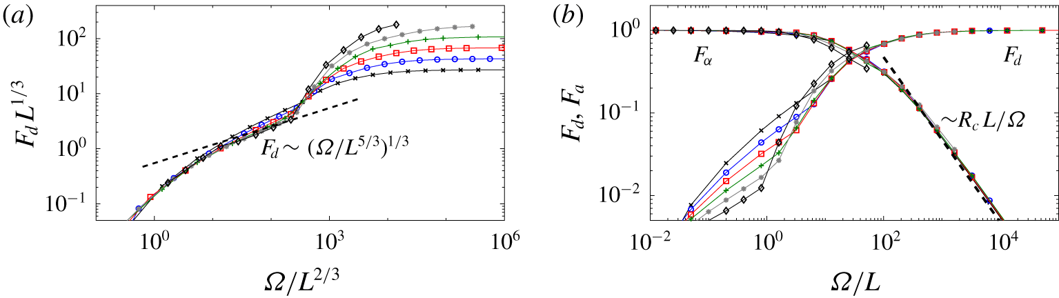
(a) The time-averaged diffusive flux  $F_{d}=\int \unicode[STIX]{x2202}c/\unicode[STIX]{x2202}z|_{z=0}\,\text{d}x$ across the low-permeability layer with the scalings in the gravity-current regime, and (b)
 $F_{d}$ and the time-averaged advective flux
 $F_{a}=-\int cv|_{z=0}\,\text{d}x=1-F_{d}$ across the layer with the scalings in the ultimate regime. The simulations have the same parameters as in figure 3. The dashed line in (a) shows the scaling indicated, while that in (b) shows the prediction of the model in the ultimate regime.

4.5.1 Convection below the layer: $\unicode[STIX]{x1D6FA}\gg L^{2/3}$

While the flow is always unstably stratified below the layer, if  $\unicode[STIX]{x1D6FA}$ is sufficiently small then the fluid can flow laterally back into the central plume before the instability has had enough time to develop into convection. A balance between the time scale for lateral advection of the current
 ${\sim}x/u$ and that for growth of an instability over the depth of the current
 ${\sim}z/c$, together with the scalings in (4.11), suggests that the flow becomes unstable below the layer once
 $\unicode[STIX]{x1D6FA}\gtrsim L^{2/3}$. Curiously, this is the same scaling of
 $\unicode[STIX]{x1D6FA}$ as for the onset of the gravity-current regime.
Evidence for the onset of convection below the layer at this scaling can be seen in the total diffusive flux  $F_{d}=\int \unicode[STIX]{x2202}c/\unicode[STIX]{x2202}z\,\text{d}x$ across the low-permeability layer (figure 11a). As
 $\unicode[STIX]{x1D6FA}$ is increased, profiles bend round towards the predicted diffusive flux in the gravity-current regime
 $F_{d}\sim (\unicode[STIX]{x1D6FA}/L^{5/3})^{1/3}$ (discussed at the end of § 4.3). However, the profiles undergo a sharp increase in slope at
 $\unicode[STIX]{x1D6FA}/L^{2/3}\approx 200$. Snapshots of the flow reveal that this transition coincides with the onset of convection below the layer. The transition can be understood because convection transports buoyancy efficiently away from the layer, causing the concentration at the layer to decrease. The concentration gradient thus steepens, and the diffusive flux across the layer increases.
This behaviour is clearly shown in plots of the horizontally integrated concentration across the layer (figure 10). Comparison of stable flow on both sides of the layer (figure 10a) with unstable flow below the layer (figure 10c) demonstrates the steepening of concentration gradients across the layer associated with the onset of convection below it. Note that the influence of convection below the layer is confined to the boundary-layer region just above the layer; as long as the flow remains stable above the layer, the bulk of the gravity current remains unaffected and well described by the model in § 4.3.
4.5.2 Convection above the layer: $\unicode[STIX]{x1D6FA}\gg R_{c}^{3/2}L^{2/3}$

As a result of the decrease in the concentration at the layer due to convection below it, the concentration difference  $\unicode[STIX]{x0394}c$ over the boundary layer at the base of the gravity current must increase. Specifically, we expect it to increase from being negligibly small relative to the concentration scale within the current itself to being comparable to it (compare figure 10a,c), and so
 $\unicode[STIX]{x0394}c\sim c\sim L^{-1/3}$. This boundary layer at the base of the current will itself become unstable to convection when the local Rayleigh number, which scales with the density difference
 $\unicode[STIX]{x0394}c$ and layer depth
 $\unicode[STIX]{x1D6FF}\sim 1/v$, exceeds a critical value
 $R_{c}=O(10^{2})$; that is,
 $c\unicode[STIX]{x1D6FF}\sim R_{c}$ or
 $\unicode[STIX]{x1D6FA}\sim R_{c}^{3/2}L^{2/3}$. This is again the same scaling with
 $L$ as the onset of the gravity-current regime, although now with a large prefactor
 $R_{c}^{3/2}$.
Thus, for  $\unicode[STIX]{x1D6FA}\gg R_{c}^{3/2}L^{2/3}$ convection acts to mix up the concentration in the current above the layer (as seen in the blunted concentration profiles above the layer in figure 10d–f), disrupting the balance
 $C(\unicode[STIX]{x1D6F9})$ in the gravity current. The convective flux associated with this mixing is
 $\unicode[STIX]{x0394}c/\unicode[STIX]{x1D6FF}\sim c^{2}/R_{c}$, as in the ultimate regime, which must be at least comparable to the downwards advective flux
 $vc$ in order to mix up the current. If we assume that these fluxes are balanced throughout the current in the transitional regime, then we gain an additional constraint linking the concentration and velocity in the current,
 $c\sim R_{c}v$. This constraint, together with the usual balances of hydrostatic pressure and Darcy’s law (as in both the gravity-current and ultimate regimes), indicates that the width, height and concentration of the current in the transitional regime are
 $$\begin{eqnarray}x_{p}\sim \unicode[STIX]{x1D6FA}R_{c}^{-1/2},\quad z\sim \unicode[STIX]{x1D6FA}R_{c}^{-1},\quad c\sim R_{c}v\sim \unicode[STIX]{x1D6FA}^{-1/2}R_{c}^{3/4},\end{eqnarray}$$
which evolve smoothly from the gravity-current scalings in (4.11) at  $\unicode[STIX]{x1D6FA}\sim R_{c}^{3/2}L^{2/3}$. The diffusive flux and the advective flux across the low-permeability layer are comparable in this regime, and both contribute to the transport of buoyancy across the layer. Note that the scalings in (4.36) are independent of the depth
 $L$ of the layer, because, unlike in the gravity-current regime, the concentration scale in the current is not imposed by the incident plume, but is rather determined by a balance between convective mixing and vertical advection throughout the current.
However, once the height of the current in (4.36b) becomes comparable with the depth of the layer,  $z\sim L$, the flow feels the effect of the upper boundary and can no longer grow unimpeded. In particular, the hydrostatic pressure head required to force fluid across the very low-permeability layer cannot continue to grow beyond this point, which means that the advective flux must decrease as
 $\unicode[STIX]{x1D6FA}$ is increased further, becoming negligible relative to the diffusive flux across the layer. This transition occurs when
 $\unicode[STIX]{x1D6FA}\sim R_{c}L$, which marks the onset of the ultimate regime discussed above, with
 $x\sim LR_{c}^{1/2}$ and
 $c\sim L^{-1/2}R_{c}^{1/4}$ as predicted in (4.20). The advective flux decreases like
 $R_{c}L/\unicode[STIX]{x1D6FA}$ in the ultimate regime, as discussed in § 4.4 above and verified in figure 11(b).
It is difficult to obtain clear evidence for the scalings of the transitional regime in numerical simulations. It is, for example, difficult to discern a clear range of  $\unicode[STIX]{x1D6FA}$ in figure 11(b) over which the diffusive and advective fluxes are comparable. This is primarily because the difference between
 $R_{c}^{3/2}L^{2/3}$ and
 $R_{c}L$ is relatively small at the values of
 $L$ that are attainable in our numerical simulations. In addition, the onset of convection above the low-permeability layer is not marked by a clear transition at a critical value of
 $\unicode[STIX]{x1D6FA}$: instead, we observe in simulations that, as
 $\unicode[STIX]{x1D6FA}$ is increased, instabilities first form above the layer only far from the downwelling central plume, from where they are then advected even further from the central plume and thus play only a minimal role in mixing the fluid above the layer. As
 $\unicode[STIX]{x1D6FA}$ is increased further, the flow becomes unstable closer and closer to the central plume, and thus convective mixing has a progressively greater influence on the dynamics of the flow above the layer. We expect this gradual transition to be reflected in a gradual change in the scalings of the data, which is difficult to observe because the values of
 $L$ and
 $\unicode[STIX]{x1D6FA}$ are not sufficiently large.
In summary, we predict that a transitional regime lies between the gravity-current regime of § 4.3 and the ultimate regime of § 4.4. While all three regimes involve a basic balance between hydrostatic pressure and Darcy’s law, and are constrained to carry a unit buoyancy flux, the key physics in each regime is different. In the gravity current, buoyancy is transported by advection across the layer, and the concentration structure and scale  $c\sim L^{-1/3}$ are set by the incident downwelling plume. In the ultimate regime, buoyancy is transported by diffusion across the layer, and the circulating flow is constrained by the depth of the layer from the upper boundary
 $z\sim L$. In the transitional regime, both advection and diffusion contribute to the buoyancy flux across the layer, there remains a net downwards volume flux across the layer, and neither the incident plume nor the depth of the layer play a dominant role in the dynamics of the flow.
5 Conclusions
In this paper, we have studied the dynamics of steady or statistically steady buoyancy-driven plumes in a two-dimensional porous medium that contains a thin, low-permeability horizontal barrier or layer. If the dimensionless thickness  $2\unicode[STIX]{x1D716}L$ and the permeability
 $\unicode[STIX]{x1D6F1}$ of the thin layer are small relative to the distance
 $L$ to the layer and the ambient permeability, respectively, then they can be incorporated into a single parameter
 $\unicode[STIX]{x1D6FA}=2\unicode[STIX]{x1D716}L/\unicode[STIX]{x1D6F1}$ that measures the layer’s impedance.
A summary of dimensionless scalings for the different regimes of flow over a low-permeability layer for  $L\gg 1$: negligible perturbation to the plume (NP: § 4.1); local perturbation to the plume (LP: § 4.2); gravity current (GC: § 4.3); transitional regime (T: § 4.5); and the ‘ultimate’ regime (U: § 4.4). Boundaries between the regimes are given by the scalings shown for the impedance
 $\unicode[STIX]{x1D6FA}$. The table gives scalings for the width
 $x_{p}$ of the plume at the low-permeability layer, together with the concentration
 $c$ and horizontal velocity
 $u$ at the layer and the height scale
 $z$ over which the flow above the layer is affected.

We explored the effect of the depth  $L$ and the impedance
 $\unicode[STIX]{x1D6FA}$ on the spread of the plume over such a layer, and the results are summarized in table 1. For
 $\unicode[STIX]{x1D6FA}\ll L^{1/3}$, the layer has a negligible effect on the plume; for
 $L^{1/3}\ll \unicode[STIX]{x1D6FA}\ll L^{2/3}$ the layer affects the pressure, but not the width, of the plume; and for
 $L^{2/3}\ll \unicode[STIX]{x1D6FA}\ll R_{c}^{3/2}L^{2/3}$ the plume spreads as a gravity current over the layer, where
 $R_{c}=O(10^{2})$ is a critical Rayleigh number. In each of these cases, we constructed analytic solutions for the spread of the plume above the low-permeability layer.
For  $\unicode[STIX]{x1D6FA}\gg R_{c}^{3/2}L^{2/3}$, instabilities above the low-permeability layer disrupt the flow and mix up lower concentrations from the layer into the over-riding gravity current. The spreading current continues to widen and deepen with increasing
 $\unicode[STIX]{x1D6FA}$. For
 $\unicode[STIX]{x1D6FA}\gg R_{c}L$ the flow fills the depth of the region above the layer, diffusion becomes the dominant buoyancy transport across the layer, and the flow becomes independent of
 $\unicode[STIX]{x1D6FA}$. We also constructed an analytic solution for the time-averaged flow above the layer in this ‘ultimate’ regime.
The physical implications of these results are clearer if we work in dimensional variables, considering a plume of buoyancy flux  $B$ falling across a thin horizontal layer located at a depth
 $L^{\ast }$. Recall that the advection–diffusion length
 $\hat{z}=\unicode[STIX]{x1D719}D^{2}\unicode[STIX]{x1D707}/(\unicode[STIX]{x1D70C}_{0}\unicode[STIX]{x1D6FC}gk_{0}^{\ast }B)$ was used as the length scale in this work, and so the dimensionless depth
 $L=L^{\ast }/\hat{z}$ can be thought of as a Rayleigh number for the plume. The thin layer has dimensionless impedance
 $\unicode[STIX]{x1D6FA}=2\unicode[STIX]{x1D700}L^{\ast }/\hat{z}\unicode[STIX]{x1D6F1}$, written in terms of the layer width
 $2\unicode[STIX]{x1D700}L^{\ast }$ and permeability ratio
 $\unicode[STIX]{x1D6F1}$. If
 $\unicode[STIX]{x1D6FA}\ll (L^{\ast }/\hat{z})^{2/3}$, the layer has a negligible impact on the spread of the plume, and the half-width of the plume at the layer is
 $x_{p}^{\ast }\approx 4.1\,L^{\ast 2/3}\hat{z}^{1/3}$. If instead
 $(L^{\ast }/\hat{z})^{2/3}\ll \unicode[STIX]{x1D6FA}\ll R_{c}^{3/2}(L^{\ast }/\hat{z})^{2/3}$, the plume spreads as a gravity current over the layer, with
 $x_{p}^{\ast }\approx 1.4\,\unicode[STIX]{x1D6FA}^{2/3}L^{\ast 2/9}\hat{z}^{7/9}$. If
 $\unicode[STIX]{x1D6FA}\gg R_{c}L^{\ast }/\hat{z}$, convection away from the layer and diffusion across it control the spread of the plume, and its mean half-width
 $x_{p}^{\ast }\approx 5.3\,L^{\ast }$ scales with the distance to the layer.
As an illustration of these results, we consider the effect on a plume of  $\text{CO}_{2}$-saturated brine falling through a saline aquifer in the context of
 $\text{CO}_{2}$ sequestration. The driving buoyancy fluxes and convective velocities are typically slow in this context: a relatively high-permeability aquifer (
 $k_{0}^{\ast }=3\times 10^{-12}~\text{m}^{2}$), for example, yields a typical convective velocity scale of
 $U\approx 10^{-6}~\text{m}~\text{s}^{-1}$ for this setting (using parameter estimates taken from the Sleipner field in the North Sea (Hewitt et al. Reference Hewitt, Neufeld and Lister2013)). Given a molecular diffusivity
 $D=10^{-9}~\text{m}^{2}~\text{s}^{-1}$ and ignoring the effects of dispersion (discussed below), the advection–diffusion length scale is thus
 $\hat{z}\approx 1~\text{mm}$. Suppose a thin layer of width
 $2\unicode[STIX]{x1D700}^{\ast }=10~\text{cm}$ lies a distance
 $L^{\ast }=10~\text{m}$ below the source of dense
 $\text{CO}_{2}$-saturated brine, so that
 $L=10^{4}$. If the thin layer has a permeability five times less than that of the aquifer, it will have a negligible effect on the spread of the plume and
 $x_{p}^{\ast }\approx 2~\text{m}$ at the layer. If, instead, the thin layer has a permeability
 $500$ times less than that of the aquifer, or even lower, it will have a dramatic effect on the layer: all the buoyancy will be transported across the layer by diffusion and the plume will spread to
 $x_{p}^{\ast }\approx 50~\text{m}$. Alternatively, if both layer and aquifer were ten times larger, so that
 $2\unicode[STIX]{x1D700}^{\ast }=1~\text{m}$ and
 $L^{\ast }=100~\text{m}$, the layer would only have to be half the permeability of the aquifer to affect the spread of the plume, but
 $700$ times less permeable to prevent advective transport.
The results of this work apply to a two-dimensional plume, and the extension to axisymmetric flow provides a natural future direction of study. One might also consider extending these models to include the effects of velocity-dependent dispersion, which can play an important role in the spreading of plumes (Sahu & Flynn Reference Sahu and Flynn2015, Reference Sahu and Flynn2016). Perhaps the most interesting extension to this work, however, would be to explore how the presence of multiple low-permeability layers affects the spread of a plume, particularly given that multiple stacked layers are common in geological settings. In particular, one might ask whether lower layers provide appreciable feedback on the dynamics of the plume at higher layers. An initial exploration of this question suggests that a system of multiple layers can give rise to a wealth of interesting dynamics, the investigation of which will be the subject of future work.
Appendix A. Numerical details
A.1 Numerical modelling
We solved the equations (2.9)–(2.10), together with the jump condition for flow across a thin low-permeability layer (2.14), numerically. To achieve this, we assumed symmetry conditions in the line  $x=0$ and worked in a finite numerical domain
 $0\leqslant x\leqslant l_{x}$ and
 $0\leqslant y\leqslant l_{y}$, for some
 $l_{x}$ and
 $l_{y}$. At the side boundary
 $x=l_{x}$, which was chosen to lie far from the extent of the plume, the pressure and solute concentration were uniform and so
 $v\equiv \unicode[STIX]{x2202}\unicode[STIX]{x1D713}/\unicode[STIX]{x2202}x=c=0$.
The buoyancy source was imposed numerically on the upper boundary ( $y=0$) by a fixed non-zero vertical concentration gradient over a small region
 $0\leqslant x<x_{b}$, where
 $x_{b}\ll L$ was chosen to be equal to a few horizontal grid lengths
 $\unicode[STIX]{x1D6FF}x$. The entire upper boundary was also impermeable, so
 $$\begin{eqnarray}\frac{\unicode[STIX]{x2202}c}{\unicode[STIX]{x2202}y}=\left\{\begin{array}{@{}ll@{}}-1/(2x_{b}) & 0\leqslant x<x_{b},\\ 0 & x_{b}\leqslant x;\end{array}\right.\quad v=\unicode[STIX]{x1D713}=0\quad \text{on }y=0.\end{eqnarray}$$
Numerical solutions were checked to ensure that they were insensitive to the precise value of  $x_{b}$. On the lower boundary of the domain we imposed
 $$\begin{eqnarray}u\equiv -\frac{\unicode[STIX]{x2202}\unicode[STIX]{x1D713}}{\unicode[STIX]{x2202}y}=0;\quad \frac{\unicode[STIX]{x2202}c}{\unicode[STIX]{x2202}y}=0\quad \text{on }y=l_{y},\end{eqnarray}$$
so that concentration could advect out but not diffuse back in. The boundary  $l_{y}$ was chosen to lie far below the low-permeability layer (in all cases, at least a distance of
 $6L$ below the layer).
In order to generate steady or statistically steady plume solutions, we solved the full time-dependent equations (2.9)–(2.10), starting either from rest with  $c(t=0)=0$ throughout the domain, or from a statistically steady solution for the same value of
 $L$ but with a different impedance. The second initial condition led to more rapid convergence to a new statistically steady state than the first.
The numerical method used a Fourier transform in the  $x$ direction, a standard second-order finite-difference discretization in the
 $y$ direction, and an alternating-direction-implicit time-stepping scheme. We employed a flux-conservative discretization, with the streamfunction and concentration located on staggered grids, and a coordinate transformation in the vertical direction to ensure that the dynamics near the upper boundary and at any internal boundaries were fully resolved without prohibitive computational cost. For the lowest values of the distance to the layer
 $L$ and the impedance of the layer, we used approximately
 $(256\,300)$ grid points in the
 $(x,y)$ directions, while for the most extreme parameter settings, we used approximately
 $(40\,962\,000)$. In all cases, we ensured that boundary layers and narrow ‘proto-plumes’ were still well resolved in the vertical and horizontal directions, respectively.
A.2 Resolving the low-permeability layer
In § 2.3, we showed that the low-permeability layer can be parameterized by a jump condition at  $y=L$ and an effective impedance
 $\unicode[STIX]{x1D6FA}$ in the limit
 $\unicode[STIX]{x1D700},\unicode[STIX]{x1D6F1}\ll 1$. Here we verify this parameterization by presenting numerical results from simulations in which the full low-permeability layer of finite depth
 $2\unicode[STIX]{x1D700}L$ and permeability
 $\unicode[STIX]{x1D6F1}$ was resolved. Continuity of pressure at the edges of the layer indicates that the horizontal velocity jumps according to
 $$\begin{eqnarray}u|_{z=(\unicode[STIX]{x1D700}L)^{-}}=\unicode[STIX]{x1D6F1}u|_{z=(\unicode[STIX]{x1D700}L)^{+}},\quad u|_{z=-(\unicode[STIX]{x1D700}L)^{+}}=\unicode[STIX]{x1D6F1}u|_{z=-(\unicode[STIX]{x1D700}L)^{-}}.\end{eqnarray}$$
We imposed these jumps directly by replacing the relevant rows of the discretized derivative matrix in the  $y$ direction with conditions that enforce the required jump in the vertical gradient of the streamfunction.
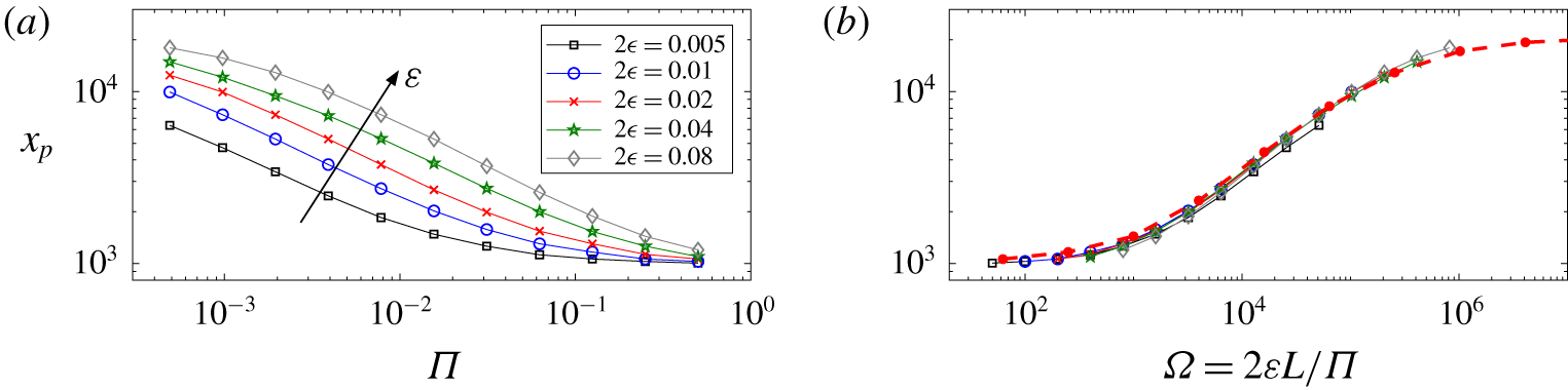
Figure 12(a) shows values of the width of the plume immediately above the layer  $x_{p}$ from simulations with different values of
 $\unicode[STIX]{x1D6F1}$ and
 $\unicode[STIX]{x1D700}$. As expected, the width increases as the thickness
 $\unicode[STIX]{x1D700}$ of the layer is increased and as the permeability
 $\unicode[STIX]{x1D6F1}$ is decreased. The data collapse when plotted as a function of
 $\unicode[STIX]{x1D6FA}$ (figure 12b), and they agree well with results from a simulation in which the layer is parameterized by the jump condition (2.14).
(a) The width  $x_{p}(\unicode[STIX]{x1D6F1})$ of the plume as defined by (3.1) from simulations in which the low-permeability layer is fully resolved, for
 $L=5\times 10^{3}$ and different layer thicknesses
 $\unicode[STIX]{x1D700}$ as marked. (b) The same data plotted as a function of the impedance
 $\unicode[STIX]{x1D6FA}=2\unicode[STIX]{x1D700}L/\unicode[STIX]{x1D6F1}$, together with solutions of the model with a jump condition at the layer (thick red dots and dashes).

Appendix B. Solution for the plume perturbation: $L^{1/3}\ll \unicode[STIX]{x1D6FA}\ll L^{2/3}$

Equation (4.10) describes the plume perturbation near the layer. Under the transformation  $Q(X,Z)=P(X,Z)\cosh X/(3\unicode[STIX]{x1D6FD}^{3})$, (4.10) reduces to the Helmholtz equation
 $$\begin{eqnarray}\frac{\unicode[STIX]{x2202}^{2}Q}{\unicode[STIX]{x2202}X^{2}}+\frac{\unicode[STIX]{x2202}^{2}Q}{\unicode[STIX]{x2202}Z^{2}}=Q;\quad Q(X,0)=\operatorname{sech}X.\end{eqnarray}$$
A Fourier transform in the  $X$ direction gives
 $$\begin{eqnarray}\tilde{Q}(k,Z)=\tilde{Q}_{0}(k)\text{e}^{-Z\sqrt{1+k^{2}}},\end{eqnarray}$$
where
 $$\begin{eqnarray}\tilde{Q}_{0}=\int _{-\infty }^{\infty }\frac{\text{e}^{-\text{i}kX}}{\cosh X}\,\text{d}X=\frac{\unicode[STIX]{x03C0}}{\cosh (\unicode[STIX]{x03C0}k/2)}.\end{eqnarray}$$
The leading-order pressure is thus
 $$\begin{eqnarray}P(X,Z)=\frac{3\unicode[STIX]{x1D6FD}^{3}}{2\cosh X}\int _{-\infty }^{\infty }\frac{\text{e}^{\text{i}Xk-Z\sqrt{1+k^{2}}}}{\cosh (\unicode[STIX]{x03C0}k/2)}\,\text{d}k=\frac{3\unicode[STIX]{x1D6FD}^{3}}{\cosh X}\int _{0}^{\infty }\frac{\cos (Xk)\text{e}^{-Z\sqrt{1+k^{2}}}}{\cosh (\unicode[STIX]{x03C0}k/2)}\,\text{d}k,\end{eqnarray}$$
which we compute numerically. The corresponding horizontal velocity is  $U=-P_{X}$, and is shown in figure 4 together with contours of the pressure
 $P$. Both quantities decay to zero as
 $Z\rightarrow \infty$, where the pressure and horizontal velocity of the plume are much smaller.