

Introduction
The basic principle of many present-day time-resolved techniques can be described as follows: A reaction is triggered in the sample, and the time-delayed probing pulse of x-rays, electrons, or neutrons creates a distinct signal (diffraction pattern, image, absorption spectrum) that can be collected at specific time delays relative to the beginning of the triggered reaction. The idea is simple and plausible, however, the technical implementation, the experimental possibilities, instrumental performance, and limitations are multiple and often challenging.
In the current scientific literature, the word “ultrashort” refers to the time domain ranging from femtoseconds (fs, 10–15 s) to picoseconds (ps, 10–12 s). Accordingly, the word “ultrafast” refers to physical, chemical, and biological events that occur on that time scale, and hence the terms femtophysics, femtochemistry, and femtobiology can be found in the recent scientific literature. Femto materials science seems to be less known, possibly because it overlaps with femtophysics and, in some aspects, with femtochemistry, because ultimately we are all trying to understand how atoms and electrons behave. Even faster processes than “femto” occur on the attosecond time scale.
This article will concentrate on the materials science aspects, taking as a given that short laser pulses (in the visible and x-ray spectral domain) can be generated. The first part of this article will present the possibilities for ultrafast materials science research. It needs to be stressed that the chief driving force for ultrafast science in physics, chemistry, biology, and materials science is the development of better, faster, brighter, and more stable lasers. Without pico-, femto-, and now attosecond laser pulses, ultrafast science would hardly be possible. The second part of this article will present two complementary and competing probing techniques (x-ray- and electron-based) that are trying to keep pace with the developments on the “laser front.”
From 3D to 4D
Although time-resolved visualization of events is not particularly new—at the beginning of the 20th century the time scale was on the order of seconds—the fascination with the new possibilities of understanding previously untraceable ultrafast physical, chemical, and biological processes, expressed in many of the associated publications, is invigorating scientists to delve into the characterization of the dynamic processes of nature.Reference Spence1–Reference Tanner and Wuttig84 In essence, one can now start to understand how the already attained three-dimensional (3D) structural information at the atomic scale changes with time—hence the terminology: structural dynamics or 4D characterization (x, y, z and time).
Electron microscopy and diffraction, x-ray and neutron diffraction, x-ray absorption, nuclear magnetic resonance, and several other spectroscopy techniques have enabled research on the structure of matter at the atomic scale. They have had an enormous impact on modern scientific knowledge by making visualization of some of the smallest building blocks of matter possible. Today, 3D structures of small molecules, crystals, biological cells, and their internal particles, nano- and micro-sized devices, can be visualized and analyzed almost at will.
As one begins to learn more about the complexity of structural changes in matter, it very quickly becomes clear that a simple structure-function correlation is indeed insufficient and often inadequate to explain and verify the mechanisms that govern structural change. In situ characterization methods in real time (milliseconds to seconds) can be performed, and they have given valuable insight into many dynamic processes involving materials.Reference Kamino, Yaguchi and Saka85–Reference Gai and Kourtakis106 Nevertheless, there are still many dynamic processes occurring in materials that are much faster than milliseconds (or video rate). They are mostly related to laser-materials interactions, since only ultrafast lasers with extremely short pulse durations (pico- to attoseconds) can excite a material into previously unknown states and conditions. In fact, there are unique and fascinating material properties and structures that can only be obtained when undergoing extremely fast processes. For example, “black silicon” is a surface modification of silicon, resulting in very low reflectivity after being irradiated by a set of laser pulses in a halogen gas environment.Reference Her, Finlay, Wu, Deliwala and Mazur107–Reference Younkin, Carey, Mazur, Levinson and Friend114 The surface of such laser-treated silicon develops a rather self-organized structure of micrometer-sized cones, and the concomitant “new” material properties include enhanced absorption, extending into the infrared spectral range below the bandgap of silicon. Pulsed laser-material interactions and their effects are multifaceted: solids are able to undergo a phase transition without appreciable heating of the bulk lattice, electron dynamics can be triggered explicitly at solid interfaces, demagnetization and a dielectric breakdown in solids can be induced,Reference Koopmans, Malinowski, Dalla Longa, Steiauf, Fähnle, Roth, Cinchetti and Aeschlimann115, Reference Rethfeld, Krutsch and Hoffmann116 and rapid phase changes can be set off locally in memory alloys and small structures. Examination of pulsed laser-treated micro- and especially nanostructures on surfaces and their size-dependent properties is as appealing as the possibilities that open up when a laser pulse is tightly focused onto a plane inside of a transparent material.Reference Feuerer and Langhoff117–Reference Vogel and Venugopalan127 Nonlinear optical absorption occurs, leading to very high temperatures and a change of the material microstructure at the focal point. This type of tailoring (or machining) of the material very locally has had some significant implications in medical applications. Corneal tissue can now be removed without any noticeable indication of thermal damage to the neighboring tissue, and functional neurosurgery could possibly also benefit from the highly localized ablation possibilities of ultrafast laser pulses. Furthermore, the extremely high intensities of such short laser pulses can cause a plethora of laser-material interactions,Reference Mourou, Tajima and Bulanov128 including laser-induced collision through electron–hole-pair excitation, double ionization, interatomic coulombic decay, stimulated scattering, soft bonding and vibrational trapping in molecules, and optically exciting non-thermal electrons in nanostructures. At subnanometer scales, the concepts of the macroscopic description of matter tend to vanish, properties can depart considerably from those of bulk matter, and the depiction of matter starts to adopt quantum mechanical descriptions, quantum states, and probability waves. Additionally, the intrinsic coherence of laser light makes it an ideal instrument to affect the coherence of an atomic or molecular system. Initial applications were focused on the tuning of chemical reactions to improve reaction yields, but the number of applications in other areas (quantum computing, quantum state preparation, and manipulation of emission of radiation in micro- and nanoscale devices involving quantum confinement) is rapidly increasing.
Time and length scales
Clearly, in order to comprehend the dynamic processes behind such interesting physical and chemical changes, the 3D structural examination before-and-after is not sufficient anymore. The substantial impact 3D structural characterization had (and still has) in the molecular and materials sciences is therefore only one part of the full picture. The other part is the dynamic aspect of matter. Electrons, atoms, molecules, and even larger living subjects such as cells tend to move and change shape, position, conformation, and possibly also composition over time—short times. There seem to be fundamental event durations that will need to be taken into account when addressing ultrafast science aspects. For example, atomic motions at the length scale of a few Angstroms take place within a few femtoseconds. Localized processes involving optical phonons, defect formation, and non-thermal melting occur in the femtosecond to picosecond time range. The ensuing events of acoustic phonon generation, structural phase transitions, and even strain propagation occur at much longer times, from nano- to microseconds. The hierarchy of length scales may therefore correlate with time scales. Common to all courses of action is that the more large-scale “global” events, occurring at later times, have their initiation at the very short times and distances.
Ultrafast conditions in matter
The physical situation in a solid when it interacts with an ultrashort laser pulse can generally be described as follows (the time scale of such process stretches over several orders of magnitude): The laser pulse impinges on the surface of a material (assume a metal), and immediately after photon absorption via inverse Bremsstrahlung, the free electrons have a non-thermal energy distribution, and therefore no specific temperature can be assigned to the system. This condition changes within the following few hundred femtoseconds as the electron gas thermalizes due to electron-electron scattering. Thermalizing involves heating the electron gas homogeneously and reaching thermal equilibrium throughout. A precise, but extremely high temperature (several thousand Kelvin) can be attributed to the system now. The ensuing transfer of energy to the lattice requires a few picoseconds, due to electron-phonon scattering. Many electron-phonon collisions are necessary—phonons are much heavier than electrons (m p/m e ~ 105)—in order to move phonons and to heat up the lattice. Here phonon mass refers to the resistance of the lattice ions to motion induced by a phonon, which is essentially a quantum mechanical description of a special type of vibrational motion, in which a lattice uniformly oscillates at the same frequency. The lattice thermalizes and approaches an equilibrium temperature afterward via phonon-phonon scattering. At sufficiently strong peak intensities, material can be ablated.
The electron-electron and the ensuing electron-phonon scattering processes have traditionally been described by a two-temperature (T) model,Reference Anisimov, Kapeliovich and Perelman129, Reference Kaganov, Lifshitz and Tanatarov130 including two separate heat capacities (C), one belonging to the excited free electron gas (T e and C e), the other to the lattice phonons (T l and C l):


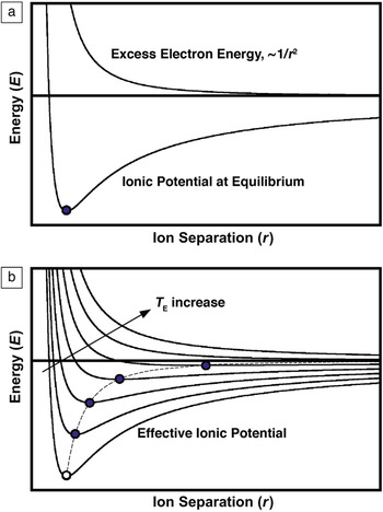
Where t is time, z is one of the three spatial coordinates, E is the absorbed laser energy, g the electron-phonon coupling constant, C e and C l the heat capacities, and k e and k l the thermal conductivities of the excited electron gas and the lattice, respectively. C e is approximately two orders of magnitude smaller than C l, and hence the increase in temperature of the bulk will be only a small fraction of the excited free electron gas temperature. However, this description is valid only when T e is known. Unfortunately, this is not the case at times shorter than 100 femtoseconds—before the electron gas thermalization. For shorter times, a model based on effective potentials needs to be used (Figure 1).Reference Rethfeld, Kaiser, Vicanek and Simon131
The effective ionic potential visualizing the reduction of the bonding energy and concomitantly an increase in ion separation caused by laser material interactions. (a) The addition of the ionic potential (at equilibrium) and the excess electron energy during excitation yields the effective ionic potential. (b) Demonstration of how the effective ionic potential changes as T E increases. The variable r is the ion separation.

Possibilities for materials science
The time domain shorter than 100 femtoseconds is becoming very interesting scientifically, and the precise absorption and electron-relaxation processes occurring in the localized volume at these extremely short times are not fully understood yet. Extremely high temperatures and pressures can be expected. The lattice may instantly disintegrate under such conditions, because a transfer of energy from the excited electrons to the lattice (electron-phonon scattering) may not be possible. The result is a direct, ultrafast solid-liquid (and/or solid-plasma) phase transformation.Reference Rethfeld, Krutsch and Hoffmann116–Reference Nolte, Momma, Chichkov and Wellig118
Under less than critical conditions but immediately after electron relaxation, the effective potential instantly takes on its new condition with a new equilibrium separation of the ions. However, the rather sluggish response of the much heavier ions to the altered effective potential, which forces the ions into new positions, results in enormous transient pressures building up in the irradiated area. The result is the generation of extremely high pressure gradients that can either disrupt the local lattice and/or send shock waves into the surrounding microstructure, causing spallation at free surfaces and interfaces that intercept the shock wave path.
The circumstances are different during the energy deposition of a nanosecond-long laser pulse. When the deposited laser energy is sufficient and the time frame long enough to establish a relatively stable temperature distribution in the sample, slightly above the melting temperature, then the sample, for example a thin film, reaches a highly local hydrodynamic state of imbalance.Reference Bostanjoglo17 Capillary forces at the surface(s) will result in shear stresses—in accordance with the dependence of the surface tension on temperature, T, and volume fraction, X, of surface impurities (e.g., oxygen), γ = γ (T, X)

Here r is the radius of the irradiated spot on the sample. Impurities will modify the surface structure by replacing lattice atoms, thus altering the surface tension characteristics. The resulting shear stresses will initiate a transport of liquid (melt) (Marangoni effect). The thermal gradient ∂T/∂r and the compositional gradient ∂X/∂r create a thermo- and/or a chemo-capillary driven flow of matter. The thermo-driven flow is given by (∂γ/∂r)X, the chemo-capillary by (∂γ/∂r)T. Accordingly, three scenarios can be distinguished as described further (see sidebar): (1) pure metals, (2) contaminated metals, and (3) over-heated thin films.
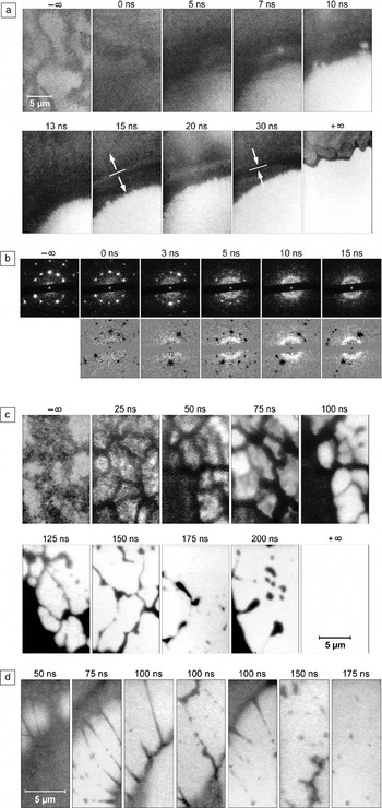
Laser pulses with high fluences can catapult a material system into regimes of extreme pressures and temperatures never attained before,Reference Mourou, Tajima and Bulanov128 and this with very high heating and cooling rates (up to 1011 K s–1). The interactions are predominantly nonlinear. The internal pressure-generating mechanisms are different at different times of observation—femto- to nanoseconds for electrons and lattice ions, respectively. Upon quenching, the material system may follow previously unknown paths of nucleation, crystallization, and grain growth. As a result, microstructures may also exhibit extraordinary material properties as in the case of “black silicon.”Reference Her, Finlay, Wu, Deliwala and Mazur107–Reference Younkin, Carey, Mazur, Levinson and Friend114 A few examples of the outcome of laser-material interactions and the material response are shown in Figure 2.
(a) Bright field images of a 30-nm-thick Ni foil during a triggered phase explosion. The untreated sample exhibits bending lines (–∞), melting (0 ns), abrupt generation of gas bubbles (5–13 ns), and expansion and compression waves (15–30 ns). The final state is indicated by +∞. Treatment laser fluence: 13.1 J/cm2, pulse duration: 6 ns. (b) (top) Single-image selected aperture diffraction demonstrates the late appearance of short-range order in a laser-treated 59-nm-thick Al foil (transition from the solid to the melt). From a plateau-like small-angle diffraction (3 ns), a diffraction ring develops (5–15 ns) that is characteristic of the newly established short-range order. In the bottom images, the diffraction pattern has been subtracted from the original, top images. Treatment laser fluence: 1.25 J/cm2, pulse duration: 6 ns. (c) Hydrodynamic effects. Creation and disintegration of the melt in a laser-irradiated 45-nm-thick Ag foil. Surface evaporation and an ensuing decomposition of the cell walls (after 100 ns) accompany the disintegration of the network. (d) The high viscosity of the melt of a laser-treated, 33-nm-thick Ge foil helps explain the formation of very long and thin melt filaments. They rupture after 75–100 ns due to a Rayleigh instability in the melt droplets (150–175 ns). Treatment laser fluence: 4.9 J/cm2, pulse duration: 6 ns. (Images courtesy of H. Dömer).

Laser-material interactions
In case (a), pure metals, there are no contaminating elements involved (X = 0), and thus thermo-capillary forces will control the shear stresses. The Gaussian shaped energy distribution of the laser pulse imposes a negative thermal gradient ∂T/∂r onto the thin film, whereas the thermal coefficient (∂γ/∂T)X = 0 is negative for pure metals. As a result, the shear stresses ∂γ/∂r are positive, pushing the molten material unidirectionally toward the colder, solid perimeter of the irradiated area. Under such conditions, a hole in the film can be created at the center of the melt.
In case (b), contaminated metals, X ≠ 0. Before, and at the beginning stages of irradiation, there is no, or no significant, gradient of the contaminating species, ∂X/∂r = 0. Contaminants are homogeneously distributed. The initial flow of material will be controlled, as in case (a) only by the thermo-capillary forces, moving outward (radial). As the energy deposition of the laser continues to heat up the thin film, a low-viscosity surface layer of melt tends to flow to the colder perimeter faster than the “bulk” material inside the film. This creates a redistribution of the impurities/contaminants (impurities are moving away from the center of the irradiated area) and thus ∂X/∂r > 0. The growing chemo-capillary force starts to counter balance the thermo-capillary force, and the initial outward flow of liquid matter may now be retarded (and even reversed). The governing parameter is the degree of surface-active contamination. The surface tension and its temperature dependence ∂γ/∂T are strongly affected by the overall impurity concentration at the film’s surface. If X >> 0, then γ(T) exhibits a local maximum at a specific temperature T 0, and the thermal coefficient (∂γ/∂T)X is positive below and negative above T 0, respectively. The laser fluence (or the deposited energy) becomes now a controlling parameter. If the temperature in the entire irradiated area remains below T 0, and with ∂T/∂r < 0, the thermo- and the chemo-capillary forces will move the melt toward the center. If T > T 0 within a certain range r < r 0, then two competing driving forces push the liquid in opposite directions. For 0 < r < r 0, the thermal coefficient (∂γ/∂T)X is negative, and the liquid flow is in many cases driven outward by the thermo-capillary force (the thermal gradient tends to be steeper than the compositional gradient, (∂T/∂r) > (∂X/∂r)). Outside this area, r > r 0, the temperature is below T 0 and (∂γ/∂T)X is positive, and concomitantly the flow of liquid directed toward the center. This scenario can result in a ring (or network) of liquid material suspended temporarily in space before it breaks apart. Depending on the dominating movement (in or outward), the ring/network (or fractions) of it may impact on the perimeter of the created hole or collapse in the center. Those dynamics can be highly complex.
In case (c), over-heated thin films, a very high temperature at the center of the irradiated area causes the surface-active impurities to vaporize right away. This results rapidly in ∂X/∂r > 0 and in addition, since the central area affected by this mechanism is relatively small, one finds that the temperature gradient for small radii ∂T/∂r here is not as steep, and therefore (∂T/∂r) < (∂X/∂r). In this case, the chemo-capillary forces dominate, driving most of the liquid toward the center and detaching it from the perimeter.

A full understanding of all relevant pulsed laser-material interactions is also very important in laser micromachining processes. For example, electronic circuit miniaturization and small microelectromechanical systems components have created a demand for better and more precise micromachining capabilities (material cutting and removal, microdrilling, microhole patterns, narrower lines, smaller and more controllable spot welding). Laser-induced quenching is also able to “freeze” a microstructure into a semi-stable state not attainable otherwise, involving, for example, high dislocation densities. This opens the possibility for precise strain engineering: a purposeful, precise placement of residual strain fields and strain-generating areas of high dislocation density, which is currently a method under consideration to further reduce the dimensions of the next generation of electronic devices.Reference Martyniuk, Antoszewski, Musca, Dell and Faraone132 Precisely positioned residual internal as well as surface strain fields can strongly affect the free carrier mobilities in semiconducting materials. Thus, the purpose of the development of ultrafast characterization methods is to begin understanding the structural dynamics associated with the creation of these novel material structures and properties.
Ultrafast time-resolved versus ultrafast pulsed experiments
The difference between the two types of experiments is that the ultrafast time-resolved process aims at gaining insight into structural dynamics, while ultrafast pulsed experiments aim at simple structural information that cannot be attained by other means. The first process was described earlier in this article, whereas the motivation for the second type of experiment is based on avoiding beam damage to the specimen. The implication of the conventional x-ray and electron-based characterization techniques is the deposition of energy by the probing beam (not the laser beam in this case, because there is no laser involved). Beam-sensitive specimens are most prone to structural damage during examination.Reference Typke, Gilpin, Downing and Glaeser133–Reference Caleman, Ortiz, Marklund, Bultmark, Gabrysch, Parak, Hajdu, Klintenberg and Tîmneanu137 Such damage is the most resolution-limiting factor in these studies, and therefore low-dose conditions need to be observed to prevent or reduce beam damage. This essentially means that the beam intensity and exposure time of the sample need to be reduced as much as possible. The consequence is a very limited amount of scattering events (x-ray or electrons) that contribute to the resulting diffraction pattern or image, and the ensuing poor signal-to-noise ratio, which limits spatial resolution and extraction of useful structural data.
One motivation for using pulsed ultrafast probes on beam-sensitive samples is therefore simply based on the concept of increasing the amount of impinging x-rays or electrons but doing so over a shorter duration to achieve better signal-to-noise ratios and better high-resolution data. Another motivation is to minimize their damaging effects, because the ultrashort probing pulse is supposed to be much faster than the damage mechanism(s). Damage is largely associated with thermal or ionization mechanisms,Reference Typke, Gilpin, Downing and Glaeser133–Reference Caleman, Ortiz, Marklund, Bultmark, Gabrysch, Parak, Hajdu, Klintenberg and Tîmneanu137 but at times, it also involves direct atom knockout.Reference Galtrey, Oliver, Kappers, Humphreys, Stokes, Clifton and Cerezo138–Reference Martin, Ishizuka, Kisielowski and Allen140 The primary requirement for the ultrafast probing pulse is thus to contain as many x-rays, photons, or electrons to achieve acceptable signal-to-noise ratios and useful data, and to be faster (shorter) than the damage mechanism(s). Further requirements are a suitable coherence of the beam and a suitable detector that can process and withstand all photon and/or electron impact.
In that sense, there is no time-delayed probing such as in the time-resolved approach to ultrafast pulsed experiments. These are single-shot experiments after which the sample may very well completely disintegrate. A repetition of the same experiment only serves the purpose of increasing the amount of critical data for high-resolution structural information—statistics, in essence. To this end, one can repeat the same experiment with multiple, yet identical, copies of the molecular structure endless times, involving no structural dynamics of interest.
The following sections will address the instrumentation used in ultrafast time-resolved, pulsed experiments. It is irrelevant what type of experiment (ultrafast time-resolved or just ultrafast pulsed) the user wants to pursue, because both methods employ the identical pulsed probe of x-rays or electrons. Ultrafast pulsed experiments require a supply of multiple, identical copies of the sample, whereas the ultrafast time-resolved process requires the experimenter to work out the pump-probe synchronization strategy.
Time-resolved characterization instrumentation
The recent technological, especially the instrumental, developments that permit addressing such fundamental research into ultrafast dynamic phenomena in material, biological, and chemical systems differ from the traditionally employed spectroscopic methods in that they attempt to visualize these processes in real space. With spectroscopic methods, two or more optical pulses with a variable time delay between them are used to investigate the processes happening during an ultrafast reaction. There is no doubt that such optical spectroscopic techniques are by far the fastest methods in terms of time resolution; however, their spatial resolution is limited due to the indirect method of observation. The observables— intensity and energy of transition—do not allow direct visualization of the process. However, these parameters can be correlated with the molecular structures involved, as long as the structures are small and relatively simple. The drawback is that it becomes exponentially more difficult and much more ambiguous as this technique is applied to larger systems. More atoms are involved, and thus more movements and many more possible atomic positions and interactions need to be considered. Adding external confinement, as in solids, and/or longer-range intermolecular forces, complicates everything even more. A solution to the dilemma of indistinct interpretation of spectral information is to collect structural information that is not as ambiguous, for example via diffraction or direct imaging methods. The options are time-resolved x-ray, electron, or neutron diffraction (in transmission or reflection mode); time-resolved electron microscopy; and time-resolved x-ray microscopy.
In diffraction mode, it is well known that every structure has a unique diffraction pattern, making structural interpretation easier and yielding much higher spatial resolution than with spectroscopic methods. The resulting diffraction pattern may also be analyzed using the coherent diffraction imaging technique to obtain an image—a method based on the Fourier transform.Reference Miao, Charalambous, Kirz and Sayre141–Reference Maia, Ekeberg, Tîmneanu, van der Spoel and Hajdu147
In imaging mode, electron microscopy exhibits the highest spatial resolution (sub-Angstrom),Reference Jia, Lentzen and Urban148–Reference Zach and Haider153 and the advantage of electrons is that they can easily be focused because they are charged particles. In comparison, x-ray microscopy suffers from limited focusing possibilities. Their best spatial resolution is approximately 15 nanometers.154
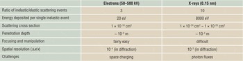
The following paragraphs will present the two most widely employed types of probes, x-rays and electrons. Table I, briefly lists their individual strengths and weaknesses.
Comparison of properties of electron and x-ray probes.

X-rays as an ultrafast probe
Instrumental developments in the past have focused on the improvement of highly intense and collimated x-ray sources—synchrotrons. Their transversal coherence is on the order of a few micrometers, and the photon fluxes achieved in such large-scale facilities (of the third generation) were 103 to 106 photons per 100 picosecond pulse. However, this is not sufficient to study atomic motions. Instead, we require the fourth generation of x-ray accelerators, called x-ray free electron lasers (XFEL), which provide up to 1012 x-ray photons in a 10 femtosecond long pulse and are therefore much better suited for ultrafast measurements. Furthermore their transverse coherence can reach several hundred micrometers.Reference Singer, Vartanyants, Kuhlmann, Duesterer, Treusch and Feldhaus155 The combination of all three parameters (coherence, amount of photons, femtosecond pulses) form a highly attractive set of parameters, ideal for structural dynamics and plain structural work on biological, chemical, and solid-state physics samples.
The amount of photons in one pulse is important, since only a sufficient amount of them will be able to form a distinguishable diffraction pattern. In crystalline structures, one can observe a strong diffraction pattern caused by elastic interaction (scattering) between the x-ray photons and the periodic lattice. Less ordered structures return Debye-Scherer rings for the same scattering process, while in amorphous matter, diffuse background scattering will dominate. In reciprocal space, x-rays can reveal precise structural information with atomic scale resolution. Time-dependent changes of position, intensity, and form (width) of the diffraction spots reveals information about structural evolutions. Increased atomic motion (or separation) due to ultrafast heating causes a shift of the diffraction spots in reciprocal space toward lower values, concomitant with an increase in the diffraction spot width, and a reduction of spot intensity. Spot displacement can be monitored fairly easily. Intensity fluctuation, on the other hand, can be a bit more challenging and relies strongly on the performance of the detector, especially its sensitivity and dynamic range. A fundamental concept in crystallography is the structure factor. A kinematical approximation for diffraction gives for the intensity I of a diffracted beam


where ψ∆k is the wave function of the beam scattered through a vector ∆k, F ∆k represents the structure factor, rj is the position (xyz)j of atom j in the unit cell, i is an imaginary number, and fj is the scattering power of that particular atom. Observation of the intensity of a specific diffraction spot will therefore reveal the unique motions of atoms drawn into the dynamic process.
Assuming that one was able to record several “useful” (non-noisy) diffraction patterns, each at a different moment in time during the ultrafast process, then the next step is the transformation from reciprocal space into real space. The difficulty here is that the relevant parameters for diffraction are amplitude and phase, and a typical diffraction pattern represents exclusively the amplitude information. The phase information is lost since the data can be collected only in terms of absolute counts of x-ray photons entering the detector. Hence, the phase retrieval is the most challenging aspect of data interpretation (the phase-problem has persisted for decades). The phase-problem is, in essence, an ill-posed inverse problem for the Fourier transformation of the data into real space (i.e., an interpretable image). Any arbitrary phase could be assigned to the amplitudes recorded prior to Fourier transformation, and any of them would return a different real-space image (and nobody knows which is correct). A few concepts have successfully been pursued in the last decade, relying on the appropriate oversampling of the recorded data and then employing iterative phase reconstruction algorithms to obtain a real space image.Reference Miao, Charalambous, Kirz and Sayre141–Reference Maia, Ekeberg, Tîmneanu, van der Spoel and Hajdu147 The same problem and methodology apply to electron and neutron diffraction patterns.
Differences between x-rays and electrons
X-rays have a fairly large penetration depth, allowing for the examination of micrometer-thick samples. This is due to their relatively small scattering cross section, about five orders of magnitude smaller than for electrons. Conversely, electrons have a 105 times stronger scattering power when interacting with matter.Reference Siwick, Dwyer, Jordan and Miller18 Considering also that electron sources are already able to emit 107 to 108 electrons in a 500 femtosecond-long pulse makes electron sources as powerful (1012 to 1013) as the novel and large-scale XFEL x-ray sources, putting out 1012 x-ray photons in a 100 femtosecond-long pulse.
X-rays are much more difficult to focus than visible light or electrons. Electrons are charged particles, and electron optical devices are highly developed tools employed in electron microscopes, achieving sub-atomic spatial resolution.
However, there are other inherent differences between x-rays and electrons when employed as a probe (see Table I). Two parameters are important: (1) the ratio of inelastic/elastic scattering events is about 3 for electrons, versus 10 for x-rays, and (2) the energy deposited per single inelastic scattering event is approximately 20 eV for electrons as compared to 8000 eV for x-rays.Reference Henderson135 Considering both, the unnecessary deposition of energy per useful elastic scattering event is more than 1000 times larger for x-rays than for electrons. This obviously makes electrons much better suited to investigate beam-sensitive specimens. Furthermore, the mean free path that electrons can travel without a single scattering event in a sample ranges from a few tens to approximately 200 nanometers in dense solids and less dense biological samples, respectively. This range matches well with the penetration depth of laser pulses meant to excite matter. It would be less useful to probe a sample area that is either above or below the “active” area.
Electrons as an ultrafast probe
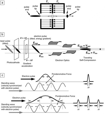
The advantages of electrons as just described are offset by a very small but significant problem. The challenge with electrons when it comes to ultrafast pulsed probes is the inherent physical law of Coulomb repulsion between charged particles (space-charging), which limits the formation and propagation of femtosecond-long electron pulses considerably.Reference Siwick, Green, Hebeisen and Miller31, Reference Siwick, Dwyer, Jordan and Miller55, Reference Siwick, Dwyer, Jordan and Miller156, Reference van Oudheusden, de Jong, van der Geer, Op’t Root, Luiten and Siwick157 Ultrashort electron pulses broaden in space and lengthen in time by orders of magnitude depending on the distance (or time) traveled and the amount of electrons they consist of. A 200 femtosecond-long, 60 kV electron pulse containing 1010 electrons/m2 quickly elongates to 2 picoseconds if traveling for about 5 nanoseconds. To avoid pulse lengthening, it may not travel for longer than 0.5 nanoseconds (Figure 3). The lateral spread in space of an “overcharged” electron pulse causes similar problems. Although electrons can be focused to spots only a few Angstroms in diameter, this does not apply anymore when several thousand electrons need to go simultaneously through focal points and crossovers only micrometers in size, as required in electron microscopes. Besides the space-charge-related effect of pulse broadening, the energy spread ∆E of the accelerated electrons (30–300 keV) will cause similar dispersion of the electron pulses. Electrons with slightly more energy are accelerated to faster speeds and will travel further than less accelerated electrons within the same electron pulse. These implications mandate short distances when employing ultrashort electron pulses. Furthermore, pulse compression techniques are required. These methods range from simple reflection of the dispersing electron pulse off flat electrostatic fields, whereby the faster electrons penetrate the field deeper and reverse direction of travel later than the slower electrons, to radio frequency (RF) cavitiesReference van Oudheusden, de Jong, van der Geer, Op’t Root, Luiten and Siwick157 and correlations between a synthetic optical field and the electron pulse (employing the effects of the ponderomotive force),Reference Baum and Zewail158 thus pushing the technical development for even shorter electron pulses (Figure 4). The ponderomotive force is the non-linear effect that an optical field can have on charged particles. Experimental setups for electron diffraction allow meeting such requirements best, since distances can be kept short and modifications to the setup can be easily implemented—from the electron source, over pulse compression elements, to the sample, and to the detector.
Electron pulse spread depends on the number of electrons, N e, it contains and the time (or distance) it travels after being emitted from the source. For example, a 200 femtosecond-long, 60 kV electron pulse containing 1010 electrons/m2, quickly elongates to 2 picoseconds if traveling for about 5 nanoseconds. To avoid pulse lengthening, it may not travel for longer than 0.5 nanoseconds. Electrons accelerated to 60 kV propagate at 1.45 × 10⁸ m/s, hence, in 0.5 nanoseconds the electrons travel 7 cm—calling for very compact experimental setups.

Electron pulse compression options: (a) Radio frequency-cavity, where fast traveling electrons at the pulse tip are retarded, whereas slow traveling electrons at the pulse end are accelerated. (b) Tilted electron pulse compression, where an accelerating potential gradient (U ± ΔU) causes an energy gradient, inducing a controlled velocity gradient facilitating traveling self-compression of the electron pulse. (c) Ponderomotive-force–based pulse compression, where a synthesized standing optical wave is velocity-synchronized with the electron pulse, and the ponderomotive force is able to shape the incoming electron pulse to extremely short electron pulses (down to attoseconds). Electron pulse duration is indicated by Δt, where t is time.

X-rays, instead, do not experience these problematic space-charge effects because they are not charged particles. However, single-electron pulses do not experience Coulomb repulsion either. They can be regarded as the ultimate non-dispersing electron pulse. They are only subject to the inherent energy spread ∆E and its consequences when accelerated. They can be employed in electron microscopes, with all the bulky electromagnetic lenses, and they can be employed for electron diffraction. Similarly to low-brightness x-ray pulses, the drawback of single-electron pulses is that single-electron scattering events are insufficient to capture the entire ultrafast laser-initiated action occurring in the sample all at once. A solution to that is to increase the repetition rate of the pulses. But even with very high repetition rates, one needs to revert to a recurring action in the sample, that is, the laser-triggered reaction in the sample needs to be reversible.Reference Baum, Yang and Zewail9, Reference Srinivasan, Lobastov, Ruan and Zewail25, Reference Zewail159 A one-time, irreversible reaction is impossible to track with just one electron (or x-ray photon). A repetitive reaction in the sample can be examined only because every time the reaction is initiated, a single-electron scattering (probing) event is recorded, contributing each time to completion of the final picture, either in diffraction or in imaging mode. At repetition rates of kHz or even MHz, the entire experiment could be concluded in less than a second, with sufficient scattering events and a useful diffraction pattern that can be evaluated. A multitude of reactions in the chemistry and biology domain are ideal candidates, as well as reversible solid-solid phase transformations and magnetic domain switching in the materials sciences. However, phase-explosions, melting, and re-crystallization events are most likely not.
There is currently no better option for these irreversible reactions in a sample than using multi-electron pulses, containing as many electrons as can be generated and also compressed into one pulse.Reference Dömer and Bostanjoglo11, Reference Dömer and Bostanjoglo34, Reference Dömer and Bostanjoglo63, Reference Dömer and Bostanjoglo73 Emission limits are currently ~1010 electrons per pulse. With such a pulse, one has only a single shot with a single multi-electron pulse to perform the entire experiment, because after that, the sample has either transformed irreversibly or has been destroyed. There are cases and experiments where the reaction is not as fast, and femtosecond pulses are not necessarily required to interrogate the time line of the process. In such cases, one can indeed revert to multi-electron pulses, where space-charge effects and pulse broadening are not as critical because the reaction time line is on the order of nanoseconds or even microseconds.Reference Dömer and Bostanjoglo34, Reference LaGrange, Campbell, Turchi and King39–Reference Armstrong, Boyden, Browning, Campbell, Colvin, DeHope, Frank, Gibson, Hartemann, Kim, King, LaGrange, Pyke, Reed, Shuttlesworth, Stuart and Torralva44, Reference Kleinschmidt, Ziegler, Campbell, Colvin and Bostanjoglo53, Reference Dömer and Bostanjoglo73 At these speeds–acknowledging space-charge effects—one can perform time-resolved electron microscopy. The high spatial resolutions as attained with non-pulsed electron microscopes cannot be achieved though, because the correlation between space (∆x) and time (∆t) resolutions involves some inherent uncertainties at the ultrafast time scale.Reference Bostanjoglo17
The question that needs to be addressed in single-shot multi-electron pulsed experiments is: how many electrons are needed to obtain a decent and interpretable signal on the detector? The single-shot multi-electron pulse type of experiment requires at least 106 to 108 electrons per pulse to generate a useful diffraction pattern or image, respectively. Diffraction is, in that sense, a purely statistical experiment in that all scattering directions have to be covered by a sufficient number of scattering events to create an interpretable pattern. The goal is to obtain an acceptable signal-to-noise ratio, which can range from 3 to 10, depending on the investigator.
Conclusion
The developments in ultrashort pulsed x-ray and electron-based methods for the pump-probe as well as for the pulsed ultrafast type of experiment have reached a point where femtosecond short pulses are attainable and controllable to a certain degree to monitor and follow atomic motions during an ultrafast process. The differences between x-rays and electrons as probes complement each other, although electrons seem to have the greater potential to probe just the active volume in a laser-pulsed specimen, since optical penetration depths and electron mean free paths overlap. Moreover the scattering power of electrons is five orders of magnitude greater than for x-rays, making pulsed electron sources as bright and powerful as novel x-ray sources, such as x-ray free electron lasers. The biggest drawback for electrons is the space-charge effects, while diffraction experiments lack the potential for real-space visualization. Efforts to solve the phase problem have been successful already, yet further developments and refinements are necessary. Both types of pulsed probes are ideal tools to remedy the radiation damage challenges encountered when investigating beam-sensitive samples.
Acknowledgments
This work was supported by the Munich Centre for Advanced Photonics (MAP).

Alexander Ziegler is employed at the Max-Planck Institute for Biochemistry in the Department of Molecular Structural Biology in Germany. He received his ms (1999) and PhD (2001) degrees from the university of California, Berkeley. He has served as an author on numerous publications and has contributed many presentations. Ziegler can be reached by tel. +49-(0)89-8578-2636; e-mail ziegler@chiochem.mpg.de.