1. Introduction
Taylor–Couette flow describes the closed fluid motion between two concentric cylinders rotating about their common axis. Various flow regimes in a parameter space based on the Reynolds numbers,
 $R_o$
and
 $R_i$
, which are defined with respect to the outer and the inner cylinder angular velocities,
 $\omega _o$
and
 $\omega _i$
, and their radii,
 $r_o$
and
 $r_i$
, as
 $R_o=\omega _o r_o (r_o-r_i)/\nu$
and
 $R_i=\omega _i r_i (r_o-r_i)/\nu$
with
 $\nu$
being the kinematic viscosity, have been identified, and this problem has long been serving as a canonical problem for studying the mechanisms of instabilities and the transition to turbulence. An early experimental overview of these flow regimes is provided by Coles (Reference Coles1976), while reviews of this flow can be found in Drazin & Reid (Reference Drazin and Reid1981), Koschmieder (Reference Koschmieder1992), Tagg (Reference Tagg1994) and Grossman, Lohse & Sun (Reference Grossman, Lohse and Sun2016). In particular, Tagg (Reference Tagg1992) compiles nearly 1500 related references, indicating the degree of researchers’ interest in this problem.
Since the seminal study by Taylor (Reference Taylor1923), it has widely been accepted that the transition from circular Couette flow to axisymmetric Taylor vortex flow (TVF) occurs near the
 $R_i$
axis in the
 $(R_o, R_i)$
space, i.e. in the region of parameter space in which
 $\mu \approx 0$
, where
 $\mu =0$
denotes the case where the outer cylinder is at rest, while the transition is taken over by three-dimensional spiral vortex flow (SVF) when the cylinders are counter-rotating (
 $\mu \approx -1$
).
In the present paper, we have a particular focus on the latter case, namely the transition to SVF due to the primary instability of circular Couette flow. The transition to SVF for the case of a finite gap between cylinders has been extensively explored theoretically as detailed by Langford et al. (Reference Langford, Tagg, Kostelich, Swinney and Golubitsky1988) with
 $0.40\lesssim \eta \lesssim 0.98$
, where
 $\eta$
is the radius ratio;
 $\eta \equiv r_i/r_o$
with
 $r_i$
and
 $r_o$
being the radii of the inner and the outer cylinders, respectively. Their analysis of the primary instabilities of SVF revealed bi-criticality resulting from the involvement of several linear unstable modes (axisymmetric and non-axisymmetric modes or non-axisymmetric modes with different azimuthal wavenumbers), which led to further studies by, for example, Golubitsky & Langford (Reference Golubitsky and Langford1988)
 $(0.43\lesssim \eta \lesssim 0.98)$
, Sánchez et al. (Reference Sánchez, Crespo and Marquès1993)
 $(\eta =0.8)$
, Antonijoan, Marquès & Sánchez (Reference Antonijoan, Marquès and Sánchez1998)
 $(\eta =0.8)$
, Hoffmann, Lücke & Pinter (Reference Hoffmann, Lücke and Pinter2004)
 $(\eta =0.5)$
, Pinter, Lücke & Hoffmann (Reference Pinter, Lücke and Hoffmann2006)
 $(\eta =0.5)$
, Meseguer et al. (Reference Meseguer, Mellibovsky, Avila and Marquès2009)
 $(\eta =0.883)$
, Goharzadeh & Mutabazi (Reference Goharzadeh and Mutabazi2010)
 $(\eta =0.883)$
and more recently Bengana & Tuckerman (Reference Bengana and Tuckerman2019)
 $(\eta =0.5)$
.
Experimental studies have included those of Snyder (Reference Snyder1970), Andereck, Liu & Swinney (Reference Andereck, Liu and Swinney1986) and Dutcher & Muller (Reference Dutcher and Muller2009), who carried out experiments relevant to the narrow-gap limit with
 $\eta =0.883, \, 0.912$
and
 $0.959$
, respectively.
Considering various aspects of theoretical and experimental investigations that have been explored for SVF in the finite-gap cases, one interesting question arises regarding how the experimental observations converge when the gap is reduced to zero (
 $\eta \rightarrow 1$
). In this so-called narrow-gap limit, the circular geometry of the cylinder walls approaches a plane geometry.
A linear stability analysis of SVF based on Cartesian geometry has been carried out by Krueger, Gross & Di Prima (Reference Krueger, Gross and Di Prima1966), who showed that the crossover of the transition from axisymmetric to three-dimensional instability takes place at
 $\mu =-0.78$
in the narrow limit of the gap (
 $\eta \rightarrow 1$
).
Weakly nonlinear analysis in the neighbourhood of this crossover point in the narrow-gap limit has been conducted by Demay, Looss & Laure (Reference Demay, Looss and Laure1992a ), Demay, Looss & Laure (Reference Demay, Iooss and Laure1992b ), Chossat et al. (Reference Chossat and Iooss1994) and Itoh (Reference Itoh1996), by extending the amplitude equation at the onset of TVF by Tabeling (Reference Tabeling1983) to the bi-critical case for a steady mode (TVF) and an oscillatory mode (SVF). Those studies are concerned with the problem of pattern formation through mode interaction.
Recently, Nagata (Reference Nagata2023, Reference Nagata2024) performed linear and nonlinear analyses, concentrating on the axisymmetric case for the narrow-gap limit. After confirming that his linear stability results agreed perfectly well with previous studies (Lin Reference Lin1955; Chandrasekhar Reference Chandrasekhar1961; Harris & Reid Reference Harris and Reid1964), nonlinear axisymmetric TVF branches bifurcating from the linear critical points were sought. He found that the bifurcation of the axisymmetric TVF is supercritical as expected for
 $-0.75\leqslant \mu \lt 1$
, while, contrary to expectations, the bifurcation nature changes to subcritical for
 $\mu \leqslant -0.75$
.
In the present study we carry out a nonlinear analysis of SVF by extending the axisymmetric analyses of Nagata (Reference Nagata2023, Reference Nagata2024) to the three-dimensional case, by taking into account those terms that are dependent on the azimuthal coordinate. Following Nagata (Reference Nagata2024), we re-scale the azimuthal coordinate by
 $1/\sqrt {1-\eta }$
and the azimuthal velocity component by
 $\sqrt {1-\eta }$
in the equations to be solved. By doing so, we are able to reproduce the linear result of Krueger et al. (Reference Krueger, Gross and Di Prima1966), and find that a spiral form of nonlinear vortex flow bifurcates from the linear critical point. In the case of
 $\mu =-1$
, the bifurcation of SVF with azimuthal wavenumber
 $\alpha \neq 0$
occurs before TVF sets in, provided that
 $\alpha$
is less than about
 $0.7$
. The boundary of existence of SVF on the scaled Reynolds number space,
 $(R_o^* , R_i^*) \equiv (\sqrt {1-\eta }R_o \, , \, \sqrt {1-\eta }R_i)$
, is determined by the saddle-node point of the subcritical SVF branch, not by the linear critical point, and is compared with the aforementioned experimental observations by Snyder (Reference Snyder1970), Andereck et al. (Reference Andereck, Liu and Swinney1986) and Dutcher & Muller (Reference Dutcher and Muller2009).
We formulate the problem of the Taylor–Couette system in the narrow-gap limit in § 2, followed by an analysis to determine the proper scalings for coordinates and variables in § 3. The results of the linear and nonlinear analyses are presented in § 4. Finally, the present study is summarised in § 5.
2. Formulation
We consider incompressible motion of a fluid with density
 $\rho$
and kinematic viscosity
 $\nu$
, which is confined between two coaxial cylinders of infinite extent in the axial direction, where the inner and outer cylinders have radii
 $r_i$
and
 $r_o$
, and rotate with angular velocities
 $\omega _i$
and
 $\omega _o$
, respectively. We assume that
 $\omega _i \neq 0$
.
Choosing a half-gap width
 $d=(r_o - r_i)/2$
as the length scale,
 $d^2/\nu$
as the time scale,
 $\nu /d$
as the velocity scale and
 $\rho \nu ^2/d^2$
as the pressure scale, we first non-dimensionalise the equations of motion in the cylindrical coordinate system, followed by transforming them into the Cartesian coordinate system, considering the narrow limit of the gap between the coaxial cylinders (
 $\eta \rightarrow 1$
).
The resultant equations of motion for non-dimensional velocity and pressure disturbances
 $(\hat {\boldsymbol u}; \hat {p}) = (\hat {u}_x, \hat {u}_y, \hat {u}_z ; \hat {p} )$
imposed on the basic velocity and pressure,
 $(U_B, 0 \, , 0 \, ; P)$
, are written in a vector form as
 \begin{align}&\qquad\qquad\qquad\qquad\qquad\qquad\quad \boldsymbol{\nabla }\boldsymbol{\cdot }\hat {\boldsymbol u} = 0, \end{align}
 \begin{align}& (\partial _t - {\nabla} ^2 ) \hat {\boldsymbol u} = - \boldsymbol{\nabla }\hat p - {U_B}\partial _x \hat {\boldsymbol u} + {\textit{Re}} \,\hat {u}_z \hat {\boldsymbol i} - \frac {1}{2} Q z \hat {u}_x \hat {\boldsymbol k} - {\varOmega } \hat {\boldsymbol j}\times \hat {\boldsymbol u} - ( \hat {\boldsymbol u} \boldsymbol{\cdot }\boldsymbol{\nabla }) \hat {\boldsymbol u}, \end{align}
where
 $\hat {\boldsymbol i}$
,
 $\hat {\boldsymbol j}$
and
 $\hat {\boldsymbol k}$
are the unit vectors in the
 $x$
(azimuthal),
 $y$
(axial) and
 $z$
(wall-normal) directions, respectively. In (2.2),
 ${\textit{Re}}$
is the Reynolds number,
 $ \varOmega$
is the rotation number and
 $Q$
represents the effect of inertia, defined by
 \begin{equation} {\textit{Re}} = \frac { \omega _i (1- \mu ) \overline {r} d }{2\nu },\quad {\varOmega } = \frac {\omega _i (1+\mu ) d^2 }{\nu } \quad \mbox{and} \quad Q = \frac {2\omega _i (1-\mu ) d^2 }{\nu }, \end{equation}
and the basic velocity component in the azimuthal direction is given by
 $U_B(z)=-{\textit{Re}} \,z$
. For the derivation of (2.1), (2.2) and (2.3), the reader is referred to Nagata (Reference Nagata2023, Reference Nagata2024). (There is a misprint in the left-hand side of (2.11) in Nagata (Reference Nagata2024):
 $ (({U}/{r})- ({{\tilde u}_\varphi }/{r}) )$
should be
 $ (({U}/{r}) + ({{\tilde u}_\varphi }/{r}))$
).
Note that we have assumed that the non-dimensional form of the azimuthal component of the disturbance velocity,
 $\tilde {u}_\varphi$
, is not as large as
 $\mathcal{O}(1/\sqrt {1-\eta })$
. Because
 $1/r$
is of
 $\mathcal{O}(1-\eta )$
when normalised by the length scale
 $d$
, the curvature term,
 $\tilde {u}^2_\varphi /r$
, in the radial component of the equation of motion in the cylindrical coordinate system,
 $(r, \varphi , \zeta )$
, could be neglected in this case. Therefore, the non-dimensional form of this term,
 $-({1}/{2})(1-\eta )\hat {u}_x^2\hat {\boldsymbol k}$
, does not appear in (2.2), It was shown in Nagata (Reference Nagata2024) that this assumption is not valid in the parameter region where the flow becomes linearly unstable. Note, however, that (2.2) is still valid for linear analysis, since this term is nonlinear.
We further separate the velocity disturbance,
 $\hat {\boldsymbol u}$
, into the
 $(x,\,y)$
-averaged parts,
 $\check {U}(t,z)\hat {\boldsymbol i}$
and
 $\check {V}(t,z)\hat {\boldsymbol j}$
, and the residual,
 $\check {\boldsymbol u}$
, whereupon the nonlinear part
 $( \hat {\boldsymbol u} \boldsymbol{\cdot }\boldsymbol{\nabla }) \hat {\boldsymbol u}$
in (2.2) can be written as
 \begin{equation} ( \hat {\boldsymbol u} \boldsymbol{\cdot }\boldsymbol{\nabla }) \hat {\boldsymbol u} = \big (\check {U}(t,z)\partial _x + \check {V}(t,z)\partial _y\big )\check {\boldsymbol u} + \big (\check {U}'(t,z)\check {\boldsymbol i} + \check {V}'(t,z)\check {\boldsymbol j} \big ) \check {v}_z +( \check {\boldsymbol u} \boldsymbol{\cdot }\boldsymbol{\nabla }) \check {\boldsymbol u}, \end{equation}
where the prime denotes differentiation with respect to
 $z$
. The decomposition (2.4) is reflected later in (3.12) and (3.13), after the variable scalings (3.5) are taken into account in § 3. In contrast to the approach of Nagata (Reference Nagata2023, Reference Nagata2024) for the axisymmetric case, where only the mean-flow modification in the streamwise (azimuthal) direction,
 $\check {U}(z)$
, was considered, we here also include the generation of the mean flow in the spanwise (axial) direction,
 $\check {V}(z)$
. We anticipate that the mean-flow modifications,
 $\check {U}(z,t)\hat {\boldsymbol i}$
and
 $\check {V}(z,t)\hat {\boldsymbol j}$
, are generated by the Reynolds stress (see (3.14) and (3.15) in § 3).
3. Analysis
From (2.3), we can find
 \begin{equation} { \varOmega } = 2\frac {1+\mu }{1-\mu } \frac {d}{\overline {r}} {\textit{Re}} \approx \frac {1+\mu }{1-\mu } (1-\eta ) {\textit{Re}} \quad (\mu \neq 1) \quad \mbox{and} \quad Q = \frac {4d}{\overline {r}} {\textit{Re}} \approx 2(1-\eta ) {\textit{Re}}, \end{equation}
where
 $d/\overline {r}=(1-\eta )/(1+\eta )\approx (1-\eta) /2$
is used. This constraint indicates that the system given by (2.1) and (2.2) is governed by
 ${\textit{Re}}$
and
 $\mu$
for a given
 $\eta$
, that is, the system is governed by only two dimensionless parameters. This fact would be clear if one realises that experiments of TVF with a given
 $\eta$
in real space are described by the two Reynolds numbers
 \begin{equation} R_i= \frac {\omega _i r_i d}{\nu } \quad \mbox{and} \quad R_o= \frac {\omega _o r_o d}{\nu }, \end{equation}
based on the inner and outer cylinders (see e.g. Andereck et al. Reference Andereck, Liu and Swinney1986). These Reynolds numbers can be expressed in terms of
 ${\textit{Re}}$
and
 $\mu$
as follows:
 \begin{equation} R_i= \frac {2\eta }{1-\mu } {\textit{Re}}\quad \mbox{and} \quad R_o= \frac {2\mu }{1-\mu } {\textit{Re}}. \end{equation}
In the present analysis, we choose
 \begin{equation} \tau =Q {\textit{Re}} = 2(1-\eta ){\textit{Re}}^2 \quad \mbox{and} \quad\mu \end{equation}
as the two independent parameters, where we call
 $\tau$
the modified Taylor number, which is clearly related to the Taylor number,
 $T= ({32}/({1-\mu})) {\textit{Re}}^2 (1-\eta )= ({16}/({1-\mu}))\tau$
, used by Krueger et al. (Reference Krueger, Gross and Di Prima1966).
Only when
 $\mu \approx 1$
can the ratio
 $ \varOmega /{\textit{Re}}$
be of
 $\mathcal{O}(1)$
as
 $\eta \rightarrow 1$
by (3.1), so that
 ${\textit{Re}}$
and
 $ \varOmega$
can take finite values, while
 $Q$
should be neglected. This case is thus reduced to rotating plane Couette flow in Cartesian geometry. Note that
 $\mu$
does not appear in the analysis. This case corresponds to the study by Nagata (Reference Nagata1986) on flow between almost co-rotating cylinders.
On the other hand, when
 $\mu$
is not close to 1,
 $ \varOmega$
is of order
 $(1-\eta )$
smaller than
 ${\textit{Re}}$
by (3.1). Since
 $Q$
is also of order
 $(1-\eta )$
smaller than
 ${\textit{Re}}$
, one might suppose that the system is reduced to that of plane Couette flow. However, this is true only when
 ${\textit{Re}}$
is of
 $\mathcal{O}(1)$
, or more precisely
 ${\textit{Re}} \ll 1/\sqrt {1-\eta }$
, as follows.
First of all,
 ${\nabla} ^2\hat {u}_x \sim {\textit{Re}}\hat {u}_z$
by the
 $x$
component of (2.2). Assuming
 $\hat {u}_z \sim \mathcal{O}(1)$
and
 ${\nabla} ^2 \sim \mathcal{O}(1)$
, we find
 $\hat {u}_x \sim \mathcal{O}({\textit{Re}})$
. From the
 $z$
component of (2.2),
 $Q\hat {u}_x$
and
 $\varOmega \hat{u}_x$
are of order
 $(1-\eta ){\textit{Re}}\hat {u}_x \sim (1-\eta ){\textit{Re}}^2$
, where we used (3.1) and
 $\hat {u}_x \sim \mathcal{O}({\textit{Re}})$
. In order for these terms to be neglected to attain plane Couette flow,
 $(1-\eta ){\textit{Re}}^2 \ll 1$
, that is,
 ${\textit{Re}} \ll 1/\sqrt {1-\eta }$
.
When
 ${\textit{Re}}\sim \mathcal{O}(1/\sqrt {1-\eta }$
), the terms with
 $Q$
and
 $ \varOmega$
as coefficients in (2.2) must be retained. In this case,
 $Q\sim \mathcal{O}(\sqrt {1-\eta } )$
and
 $\varOmega \sim \mathcal{O}(\sqrt {1-\eta } )$
by (3.1), and the products
 ${\textit{Re}} \varOmega$
and
 ${\textit{Re}} Q$
are of
 $\mathcal{O}(1)$
. In fact, the linear stability analysis for the axisymmetric case by Nagata (Reference Nagata2024) showed that the product
 ${\textit{Re}} \varOmega$
or
 ${\textit{Re}} Q$
, and so the modified Taylor number (3.4), takes a finite value at the linear criticality in good agreement with Krueger et al. (Reference Krueger, Gross and Di Prima1966). Thus, the scaling discussion below follows as a consequence of the linear stability results rather than being imposed as a premise.
We anticipate that the linear criticality of the non-axisymmetric case also occurs in the region near
 ${\textit{Re}}\sim \mathcal{O}( 1/\sqrt {1-\eta } )$
and
 ${ \varOmega }\sim \mathcal{O}( \sqrt {1-\eta } )$
and the nonlinear disturbance velocity can be scaled there as
 $(\hat {u}_x, \hat {u}_y, \hat {u}_z)\sim ( \mathcal{O}(1/\sqrt {1-\eta } ), \mathcal{O}(1), \mathcal{O}(1) )$
, as in the axisymmetric case which was investigated in Nagata (Reference Nagata2024). We see that the following scaling is adequate in the region where
 ${\textit{Re}}\sim \mathcal{O}(1/\sqrt {1-\eta })$
for the non-axisymmetric case:
 \begin{align} & {\textit{Re}}^*=\sqrt {1-\eta }\,{\textit{Re}}, \quad { \varOmega ^*} = \big(1/\sqrt {1-\eta } \big)\,{ \varOmega }, \quad Q^*= \big(1/\sqrt {1-\eta } \big)\,Q, \,\, \nonumber\\ & U_B^*(z^*)=\sqrt {1-\eta } \,{U}_B(z), \quad \check {U}^*(z^*)=\sqrt {1-\eta } \,\check {U}(z), \quad \check {V}^*(z^*)=\check {V}(z), \quad p^*={\hat {p}}, \,\, \nonumber\\& \big( {\hat u}^*_{x^*}, \, {\hat u}^*_{y^*}, \,{\hat u}^*_{z^*} \big)= \big( \sqrt {1-\eta }\,{\hat u}_x, \,{\hat u}_y, \,{\hat u}_z \big), \quad (x^*,\,y^*,\,z^*) = \big(\sqrt {1-\eta }\,x, \,y,\,z \big), \end{align}
in which
 $U^*_B(z^*)=-{\textit{Re}}^*z^*$
. The coordinate scaling
 $(x^*, y^*, z^*)=(\sqrt {1-\eta }\,x, y, z)$
in (3.5), which was not considered for the axisymmetric case
 $(\partial _x\equiv 0)$
, is now required for the non-axisymmetric case (
 $\partial _x\neq 0$
), because the terms with operators such as
 $\hat {U}\partial _x$
and
 $\hat {u}_x\partial _x$
in (2.2) must balance with other terms of
 $\mathcal{O}(1)$
.
From (3.5), we see that
 \begin{equation} { \varOmega }^*= \frac {1+\mu }{1-\mu }{\textit{Re}}^* \quad \mbox{and} \quad Q^*=2{\textit{Re}}^*, \end{equation}
and
 \begin{equation} {\textit{Re}}^*Q^*={\textit{Re}}Q. \end{equation}
Both
 ${\textit{Re}}^*$
and
 $Q^*$
are now
 $\mathcal{O}(1)$
quantities and their product,
 ${\textit{Re}}^*Q^*$
, retains the same value as the product of unscaled
 ${\textit{Re}}$
and
 $Q$
, so that the modified Taylor number
 $\tau$
defined in (3.4) is still expressed by the product of
 ${\textit{Re}}^*$
and
 $Q^*$
as
 $ \tau = {\textit{Re}}^* Q^*$
.
In the region for
 ${\textit{Re}}\sim \mathcal{O}(1/\sqrt {1-\eta })$
, the curvature disturbance term in the wall-normal direction,
 $-({1}/{2})(1-\eta )\hat {u}_x^2\hat {\boldsymbol k}$
, which has been ignored in (2.2), is scaled as
 $-({1}/{2})(\hat {u}^*_{x^*})^2\hat {\boldsymbol k}$
of
 $ \mathcal{O}(1)$
, and becomes comparable to the other quadratic nonlinear terms
 $(\hat {u}^*_{x^*} \partial _{x^*} +\hat {u}^*_{y*} \partial _{y^*} + \hat {u}^*_{z^*} \partial _{z^*} )\hat {u}^*_{z^*}$
of
 $\mathcal{O}(1)$
.
By incorporating
 $-({1}/{2})(\hat {u}^*_{x^*})^2\hat {\boldsymbol k}$
, we finally obtain the equations to be solved:
 \begin{align}&\qquad\qquad\qquad\qquad \boldsymbol{\nabla} ^* \boldsymbol{\cdot }\hat {\boldsymbol u}^* = 0, \end{align}
 \begin{align} \big(\partial _t - {\boldsymbol{\nabla} ^*}^2 \big) \hat {\boldsymbol u}^* &= - \boldsymbol{\nabla} ^* p^* - {U}_B^*\partial _{x^*} \hat {\boldsymbol u}^* + {{\textit{Re}}^*} \,\hat {u}^*_{z^*} \hat {\boldsymbol i} - \frac {1}{2} Q^* z^* \hat {u}^*_{x^*} \hat {\boldsymbol k} -\frac {1}{2}\big(\hat {u}^*_{x^*} \big)^2\hat {\boldsymbol k} \nonumber\\ &\quad - {\varOmega }^* \hat {\boldsymbol j}\times \hat {\boldsymbol u}^* - \big( \hat {\boldsymbol u}^* \boldsymbol{\cdot }\boldsymbol{\nabla} ^* \big) \hat {\boldsymbol u}^*. \end{align}
Note that some unnecessary terms with
 $x^*$
derivatives have been included in the above for formality’s sake, such as
 $(1-\eta )\partial ^2_{x^*x^*}$
in
 ${\boldsymbol{\nabla} ^*}^2$
which is
 $\partial ^2_{xx}$
of
 $\mathcal{O}(1-\eta )$
before scaling and should not be included. For clarity, asterisks
 $ (\boldsymbol{\cdot })^*$
on the spatial coordinates and their derivatives are omitted hereafter.
As we mentioned in § 2, we separate the velocity perturbation
 $\hat {\boldsymbol u}^*$
into the modification,
 $\check {U}^*(z,t){\boldsymbol i}$
and
 $\check {V}^*(z,t){\boldsymbol j}$
, of the mean flows in the streamwise and spanwise directions, respectively, and a residual (periodic in space),
 $\check {\boldsymbol u}^*$
, which can be expressed in terms of poloidal and toroidal parts:
 \begin{equation} \check {\boldsymbol u}^*= (\check u^*, \check v^*, \check w^* ) = \boldsymbol{\nabla }\times \big(\boldsymbol{\nabla }\times \hat {\boldsymbol k}\phi \big) + \boldsymbol{\nabla }\times \hat {\boldsymbol k}\psi = \big(\partial ^2_{xz}\phi + \partial _y \psi , \partial ^2_{yz}\phi - \partial _x \psi , -\varDelta _2 \phi \big), \end{equation}
where
 $\varDelta _2 = \partial ^2_{xx} + \partial ^2_{yy}$
. Note that the continuity equation is then satisfied automatically. Also, note that the
 $(x , y)$
average of
 $ \check {\boldsymbol u}^*$
vanishes by the periodicity assumption:
 \begin{equation} \overline { \check {\boldsymbol u}^*}=\overline {\phi }=\overline {\psi }=0, \end{equation}
where the overline indicates the
 $(x ,y)$
average.
After applying the scaled version of (2.4) to the nonlinear term,
 $( \hat {\boldsymbol u}^* \boldsymbol{\cdot }\boldsymbol{\nabla} ^*) \hat {\boldsymbol u}^*$
, in (3.9), we operate
 $\hat {\boldsymbol k}\boldsymbol{\cdot }\boldsymbol{\nabla }\times \boldsymbol{\nabla }\times \,$
and
 $\hat {\boldsymbol k}\boldsymbol{\cdot }\boldsymbol{\nabla }\times$
on (3.9):
 \begin{align} \partial _t {\nabla} ^2\varDelta _2\phi &= \big( \boldsymbol{\nabla} ^4 + \big(U^*_B+\check {U}^* \big){}''\partial _x +\check {V}^*{}''\partial _y - \big(U^*_B+\check {U}^* \big) \partial _x {\nabla} ^2 - \check {V}^*\partial _y {\nabla} ^2 \big ) \varDelta _2 \phi \nonumber \\&\quad + \frac {1}{2} Q^* z \varDelta _2 \big(\partial ^2_{xz}\phi + \partial _y \psi \big) + \frac {1}{2}\varDelta _2 \big( 2\check {U}^* \partial _y\psi + \partial _y \psi \partial _y \psi \big) \nonumber \\ &\quad - \varOmega ^* \partial _y \varDelta _2\psi -\hat {\boldsymbol k}\boldsymbol{\cdot }\boldsymbol{\nabla }\times \boldsymbol{\nabla }\times [\check {\boldsymbol u}^*\boldsymbol{\cdot }\check {\boldsymbol u}^*], \\[-9pt] \nonumber \end{align}
 \begin{align} \partial _t \varDelta _2\psi & =\big ( {\nabla} ^2 - \big(U_B^*+\check {U}^* \big)\partial _x - \check {V}^* \partial _y \big ) \varDelta _2 \psi \nonumber \\&\qquad\qquad + \big ( \big(U^*_B+\check {U}^* \big)'\partial _y - \check {V}^* {}' \partial _y \big ) \varDelta _2\phi +\hat {\boldsymbol k}\boldsymbol{\cdot }\boldsymbol{\nabla }\times [\check {\boldsymbol u}^*\boldsymbol{\cdot }\check {\boldsymbol u}^*]. \end{align}
The two terms of the second line in (3.12) correspond to the effect of the inertia. Since
 $z$
is odd, the former breaks the symmetry in
 $z$
.
The equations for
 $\check {U}^*(z)$
and
 $\check {V}^*(z)$
are obtained by averaging the
 $x$
and
 $y$
components of (3.9) in
 $(x,y)$
space, respectively:
 \begin{align}& \partial _t \check {U}^*= \check {U}^*{''} + \partial _z \overline { \varDelta _2 \phi ( \partial ^2_{xz}\phi + \partial _y \psi } ), \\[-9pt] \nonumber \end{align}
 \begin{align}& \partial _t \check {V}^*= \check {V}^*{''} + \partial _z \overline { \varDelta _2 \phi ( \partial ^2_{yz}\phi - \partial _x \psi } ). \end{align}
This shows that
 $\check {U}^*$
and
 $\check {V}^*$
are created by the Reynolds stress. Note that
 $\varDelta _2 \phi =-\check {w}^*$
and
 $\partial ^2_{xz}\phi + \partial _y \psi = \check {u}^*$
and
 $\partial ^2_{yz}\phi - \partial _x \psi = \check {v}^*$
by (3.10).
The no-slip boundary conditions become
 \begin{equation} \phi =\partial _z \phi =\psi =\check {U}^*=\check {V}^*= 0 \quad \mbox{at} \quad z=\pm 1. \end{equation}
Note again that unnecessary terms with the
 $x$
derivatives have been included in (3.10)–(3.15).
We also note that in deriving (3.15) we followed Antonijoan et al. (Reference Antonijoan, Marquès and Sánchez1998) for the finite-gap case, which featured a non-zero total axial flux, which is not realistic in usual experiments with cylinders of finite length with lids at both ends. In order to be compatible with experiments with closed ends, we could add a constant vertical pressure gradient on the right-hand side of (3.15), as suggested by Edwards et al. (Reference Edwards, Tagg, Dornblaser, Tuckerman and Swinney1991). (This suggestion is an application of Saffman (Reference Saffman1983) on which constraint to be imposed, with the flux kept constant or with the pressure gradient kept constant in the streamwise direction for the formulation of channel flow, to Taylor–Couette flow in the axial direction.) And we could impose zero axial flux, so that the added unknown axial pressure gradient and the imposed zero axial flux compensate to solve the system of equations of motion. However, the nonlinear calculations by Sánchez et al. (Reference Sánchez, Crespo and Marquès1993) for the finite-gap case showed solutions with the included axial pressure gradient are almost identical to those without.
Although it is early to say that the two types of solutions, one with the zero-axial-flux constraint and the other without, are almost identical in the narrow-gap limit case as well, the current analyses below use (3.15) as it stands, allowing an axial flux. The reason for this choice is that we could expect that the two types of solutions do not differ much in the region of our interest, not very far from the linear criticality where they are identical, and that the imposition of zero axial flux is not sufficient for analyses to be compatible with experiments. In fact, in order for analyses to be more compatible with experiments, the axial periodicity condition must be replaced by the no-penetration condition at both ends, which is out of our current scope.
4. Results
4.1. Linear stability analysis
The infinitesimal non-axisymmetric perturbations,
 $\tilde \phi$
and
 $\tilde \psi$
, imposed on the basic circular Couette flow solution,
 $U^*_B(z)=-{\textit{Re}}^*z$
, are expanded as follows:
 \begin{align}& \tilde {\phi } ( x, y, z, t) =\sum _{l=0}^{L} \tilde {\phi }_{l} \exp [{\textrm i} (\alpha x + \beta y) +\sigma t] \big(z^2-1\big)^2 T_l (z), \end{align}
 \begin{align}& \tilde {\psi }( x, y, z, t) =\sum _{l=0}^{L} \tilde {\psi }_{l} \exp [{\textrm i} (\alpha x + \beta y) +\sigma t] \big(z^2-1\big) T_l (z). \end{align}
Here, in order for no-slip boundary conditions (3.16) to be satisfied, the Chebyshev polynomial
 $T_l (z)$
is multiplied by
 $(z^2 -1)^2$
for
 $\tilde \phi$
and
 $(z^2-1)$
for
 $\tilde \psi$
.
These non-axisymmetric perturbations satisfy
 \begin{align} \partial _t \big(\partial ^2_{yy} + \partial ^2_{zz} \big) \partial ^2_{yy} \tilde {\phi } &= \Big ( \big(\partial ^2_{yy} + \partial ^2_{zz} \big)^2 + U^*_B {}''\partial _x - U^*_B \partial _x \big(\partial ^2_{yy} + \partial ^2_{zz} \big) \Big ) \partial ^2_{yy} \tilde {\phi } \nonumber \\& \quad + \bigg ( \frac {1}{2}z\,Q^* - \varOmega ^* \bigg ) \partial ^3_{yyy} \tilde{\psi} , \\[-9pt] \nonumber \end{align}
 \begin{align} \partial _t \partial ^2_{yy} \tilde {\psi } &= \big ( \big(\partial ^2_{yy} + \partial ^2_{zz} \big) -U^*_B\partial _x \big ) \partial ^2_{yy} \tilde {\psi } -{\textit{Re}}^* \partial ^3_{yyy} \tilde {\phi }. \\[9pt] \nonumber \end{align}
Upon taking the
 $(x,y)$
average of (4.3) and (4.4), followed by evaluating the average at the internal collocation points in the wall-normal direction,
 \begin{equation} z_j = \cos \frac {j\pi }{L+2} \quad (j=1, \dots , L+1), \end{equation}
the resulting linear algebraic equations for the amplitudes
 $\tilde {\phi }_{l}$
and
 $\tilde {\psi }_{l}$
are solved as an eigenvalue problem for the complex growth rate
 $\sigma$
of perturbations
 $\tilde {\phi }$
and
 $\tilde {\psi }$
.
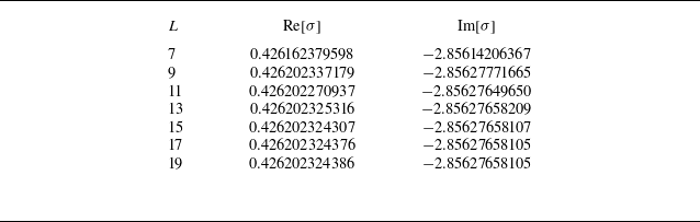
In table 1, we check the convergence of the complex eigenvalue
 $\sigma = \sigma ^R + {\textrm i}\sigma ^I$
, where
 $\sigma ^R$
and
 $\sigma ^I$
denote the real and the imaginary parts,
 ${\textrm{Re}} [\sigma ]$
and
 ${\textrm{Im}} [\sigma ]$
, of
 $\sigma$
, respectively, for non-axisymmetric perturbations with respect to the truncation level
 $L$
of the Chebyshev polynomials when
 $\mu =-1$
. The parameter values are
 $\alpha =0.2$
and
 $\beta =2.0$
at
 $\tau =2450$
. The truncation level
 $L=19$
is used in the following calculations.
Convergence of the eigenvalue
 $\sigma =(\sigma ^{R}+{\textrm i} \sigma ^{I} )$
with respect to the truncation level
 $L$
at
 $\tau =2450$
. Here
 $\alpha =0.2$
,
 $\beta =2.0$
and
 $\mu =-1$
.

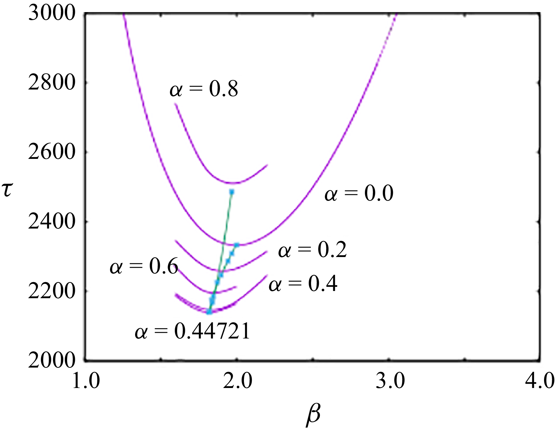
The neutral curves
 $\tau =\mathcal{N}_\alpha (\beta )$
for given values of
 $\alpha$
are shown in figure 1. In particular, we show the neutral curve
 $\tau =\mathcal{N}_0(\beta )$
for the axisymmetric case
 $\alpha =0$
, while for the values
 $\alpha =0.2,\ 0.4,\ 0.44721,\ 0.6$
and 0.8 we show the part of the neutral curves
 $\tau =\mathcal{N}_\alpha (\beta )$
close to their critical points. Also shown in the figure by points is the critical Taylor number,
 $Tc(\mu ,k)$
, for various azimuthal wavenumbers,
 $k$
, for
 $\mu =-1$
listed in table 1 of Krueger et al. (Reference Krueger, Gross and Di Prima1966). These points are connected in increasing order of
 $k$
starting from that at
 $k=0$
by converting their
 $T$
and
 $k$
to our
 $\tau$
and
 $\alpha$
via
 $T=16\tau /(1-\mu )$
and
 $k=\alpha$
.
Neutral curves for axisymmetric disturbance (
 $\alpha =0$
) and non-axisymmetric mode (
 $\alpha \neq 0$
) for
 $\mu =-1$
. The critical points
 $T_c(\mu ,k)$
for
 $\mu =-1$
listed in table 1 of Krueger et al. (Reference Krueger, Gross and Di Prima1966) are converted to our
 $\tau _c(\alpha )$
and plotted by points.

Let
 $\tau _c^{\textit{min}}$
denote the value of
 $\tau$
at the lowest point of each of the neutral curves
 $\mathcal{N}_\alpha (\beta )$
for
 $\alpha$
. Detailed calculations for
 $\mu =-1$
show
 $\tau _c^{\textit{min}}=2332.824$
for
 $\alpha =0$
when
 $\beta =1.999$
and
 $\tau _c^{\textit{min}}=2140.82$
for
 $\alpha =0.44721$
when
 $\beta =1.821$
. These values can be compared with those listed in Krueger et al. (Reference Krueger, Gross and Di Prima1966). (Their definition of the Taylor number is given by
 $T\sim 2(1-\mu )(\omega _i r_i D/\nu )^2 D/r_i )$
where
 $D=2d$
(see (5) in Krueger et al. (Reference Krueger, Gross and Di Prima1966)). From (3.4) and
 ${\textit{Re}}^*=\sqrt {1-\eta }{\textit{Re}}$
in (3.5), we get
 $\tau =2({\textit{Re}}^*)^2$
. Substitution of (3.3) leads to
 $T=16\tau /(1-\mu )$
.) They obtained the critical values by solving an eigenvalue problem for a relevant six-order system by the Runge–Kutta method. Their values were
 $T_c=18669 (\times (({1-\mu})/{16})=2333.625$
) for the critical wavenumber
 $\beta _c$
= 3.999(/2 = 1.9995) at
 $\alpha =0$
and
 $T_c=17129 (\times (({1-\mu})/{16})=2141.125$
) for
 $\beta _c$
= 3.642(/2 = 1.821) at
 $\alpha =0.44721$
(their figures are converted to our
 $\tau$
in the parentheses).
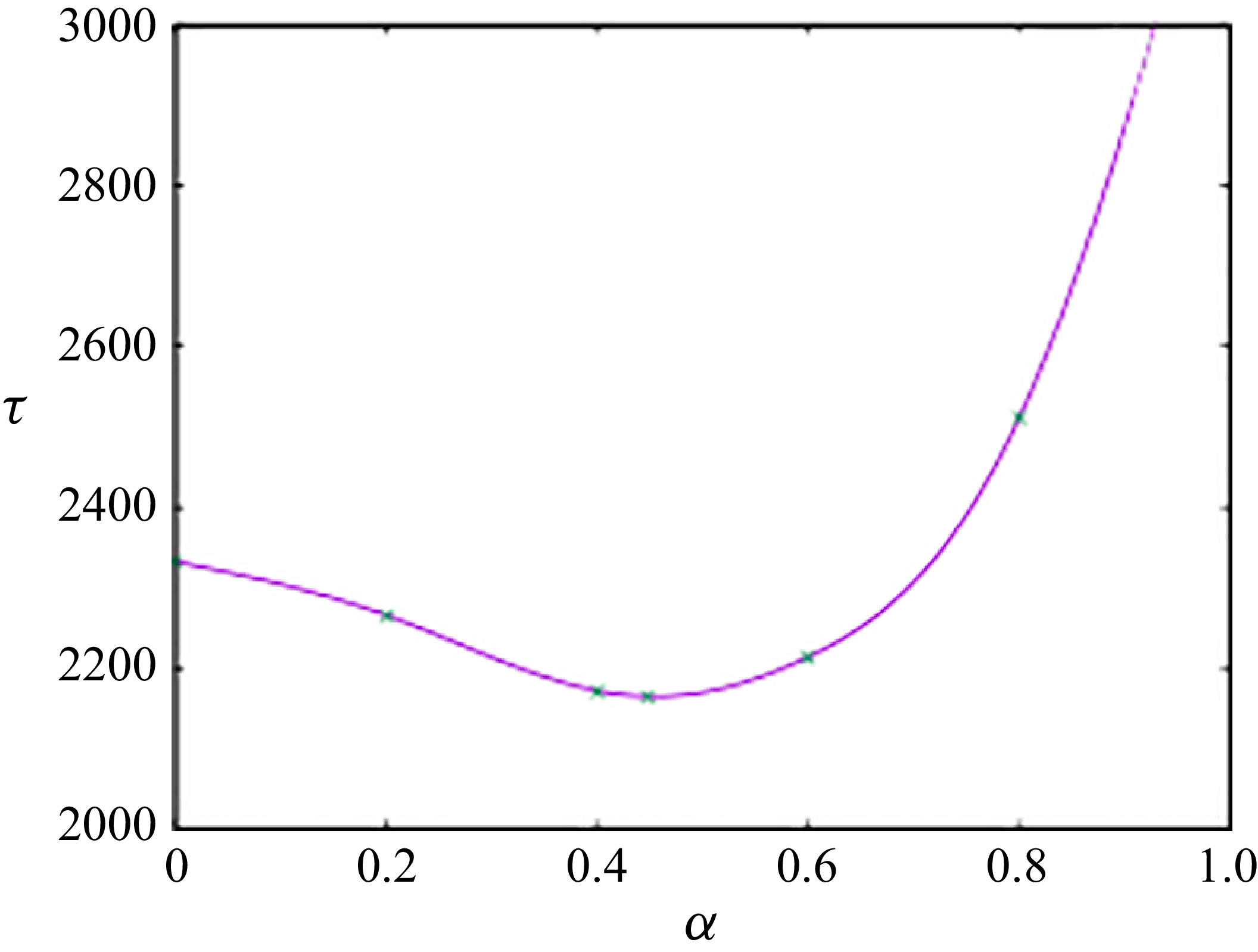
Let
 $\tau _c(\alpha )$
be the value of
 $\tau$
at the intersection points of the vertical line
 $\beta =2.0$
and the neutral curves
 $\mathcal{N}_\alpha (\beta )$
for
 $\alpha$
in figure 1. The critical value,
 $\tau _c(\alpha )$
, is plotted for
 $\beta =2.0$
when
 $\mu =-1$
in figure 2. From the figure, it is seen that, as
 $\alpha$
is increased from zero,
 $\tau _c(\alpha )$
decreases at first, takes its minimum value at
 $\alpha \approx 0.45$
and then increases sharply passing the value
 $\tau _c(0)$
for the axisymmetric case at
 $\alpha \approx 0.7$
. This critical value
 $\tau _c(\alpha )$
is slightly different from the value of
 $\tau _c^{\textit{min}}$
at the lowest point of each of the neutral curves
 $\mathcal{N}_\alpha (\beta )$
for
 $\alpha$
. This is why figure 2 is slightly different from the corresponding plot for
 $\mu =-1$
in figure 1 of Krueger et al. (Reference Krueger, Gross and Di Prima1966), where the values of
 $\tau _c^{\textit{min}}$
are evaluated against
 $\alpha$
.
The critical modified Taylor number
 $\tau _c(\alpha )$
for
 $\beta =2.0$
when
 $\mu =-1$
. (When
 $\alpha =0.44721$
,
 $\tau _c=2165$
for
 $\beta =2.0$
while
 $\tau _c=2141$
for
 $\beta =1.821$
.)

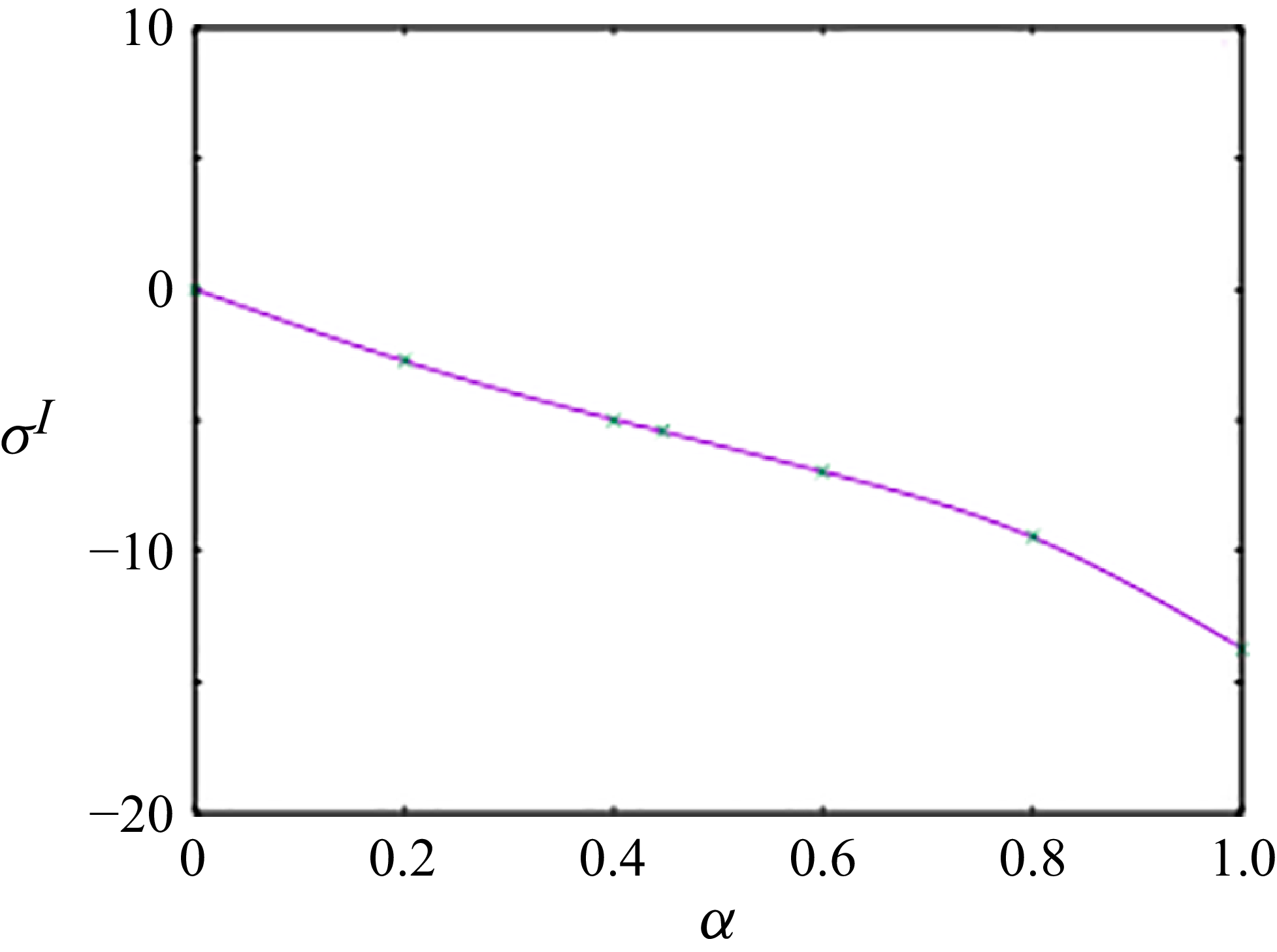
The imaginary part
 $\sigma ^I$
of
 $\sigma$
at the critical point
 $\tau _c(\alpha )$
is plotted for non-axisymmetric cases
 $\alpha \neq 0$
for
 $\beta =2.0$
in figure 3. It is no longer zero for these non-axisymmetric disturbances, decreasing from zero as
 $\alpha$
is increased from zero. The fact that the eigenvalue
 $\sigma$
at the critical point is single pure imaginary leads us to anticipate that the nonlinear three-dimensional solution, which bifurcates from that point, possesses a travelling-wave form. We show in figure 5 below that the imaginary part
 $\sigma ^I$
at the critical point is connected to the nonlinear phase speed of bifurcating SVF at its onset.
The imaginary part
 $\sigma ^I$
of the eigenvalue
 $\sigma$
at criticality
 $\tau _c (\alpha )$
. The axial wavenumber
 $\beta$
is fixed at 2.0 while
 $\mu =-1$
. (When
 $\alpha =0.44721$
,
 $\sigma ^I=-5.436$
for
 $\beta =2.0$
while
 $\sigma ^I=-5.3243$
for
 $\beta =1.821$
.)

4.2. Nonlinear analysis
The nonlinear system of equations satisfying (3.12)–(3.15) is rewritten below. Here, the terms with the
 $x$
derivatives are expressed explicitly when they are necessary:
 \begin{align}& \partial _t \big(\partial ^2_{yy}+\partial ^2_{zz}\big) \partial ^2_{yy}\phi = \Big ( \! \big(\partial ^2_{yy}+\partial ^2_{zz}\big)^2 +\big(U^*_B+\check {U}^*\big){}''\partial _x +\check {V}^*{}''\partial _y \nonumber \\&\qquad\qquad\qquad\qquad - \big(U^*_B+\check {U}^* \big) \partial _x \big(\partial ^2_{yy}+\partial ^2_{zz}\big) - \check {V}^*\partial _y \big(\partial ^2_{yy}+\partial ^2_{zz}\big) \Big ) \partial ^2_{yy} \phi \nonumber \\&\qquad\qquad\qquad\qquad + \frac {1}{2} Q^* z \partial ^2_{yy} \big(\partial ^2_{xz}\phi + \partial _y \psi \big) + \frac {1}{2}\partial ^2_{yy}\big( 2\check {U}^* \partial _y\psi + \partial _y \psi \partial _y \psi \big) \nonumber \\&\qquad\qquad\qquad\qquad - \varOmega ^* \partial _y \partial ^2_{yy}\psi -\hat {\boldsymbol k}\boldsymbol{\cdot }\boldsymbol{\nabla }\times \boldsymbol{\nabla }\times [\check {\boldsymbol u}^*\boldsymbol{\cdot }\check {\boldsymbol u}^*], \end{align}
 \begin{align} \partial _t \partial ^2_{yy}\psi & = \Big ( \! \big(\partial ^2_{yy}+\partial ^2_{zz}\big) - \big(U_B^*+\check {U}^*\big)\partial _x - \check {V}^* \partial _y \Big ) \partial ^2_{yy} \psi \nonumber \\&\qquad + \big (\big(U^*_B+\check {U}^*\big)'\partial _y - \check {V}^* {}' \partial _y \big ) \partial ^2_{yy}\phi +\hat {\boldsymbol k}\boldsymbol{\cdot }\boldsymbol{\nabla }\times [\check {\boldsymbol u}^*\boldsymbol{\cdot }\check {\boldsymbol u}^*], \\[-9pt] \nonumber \end{align}
 \begin{align}\partial _t \check {U}^* & = \check {U}^*{''} + \partial _z \overline { \partial ^2_{yy} \phi \, \partial _y \psi }, \\[-9pt] \nonumber \end{align}
 \begin{align} \partial _t \check {V}^* & = \check {V}^*{''} + \partial _z \overline { \partial ^2_{yy} \phi ( \partial ^2_{yz}\phi - \partial _x \psi } ). \\[9pt] \nonumber \end{align}
Note that
 \begin{equation} \check {u}^*_x= \partial _y \psi , \quad \check {u}^*_y = \partial ^2_{yz}\phi - \partial _x \psi \quad \mbox{and} \quad \check {u}^*_z = - \partial ^2_{yy} \phi \end{equation}
for the narrow-gap limit case
 $\eta =1$
by (3.5). It is interesting to realise that the disturbance velocity
 $\check {\boldsymbol u}^*$
can be expressed by two streamfunctions: one,
 $\psi$
, in the
 $(x,y)$
plane and the other,
 $\varPsi \equiv \phi _y$
, in the
 $(y,z)$
plane.
The no-slip boundary conditions become
 \begin{equation} \phi =\partial _z \phi =\psi =\check {U}^*=\check {V}^*= 0 \quad \mbox{at} \quad z=\pm 1. \end{equation}
The nonlinear interaction terms
 $\hat {\boldsymbol k}\boldsymbol{\cdot }\boldsymbol{\nabla }\times \boldsymbol{\nabla }\times [\check {\boldsymbol u} ^*\boldsymbol{\cdot }{ \check {\boldsymbol u}^*}]$
in (4.6) and
 $\hat {\boldsymbol k}\boldsymbol{\cdot }\boldsymbol{\nabla }\times [\check {\boldsymbol u}^*\boldsymbol{\cdot }{ \check {\boldsymbol u}^*}]$
in (4.7) are expressed explicitly in Appendix A.
From the time-dependent form of linear perturbations, (4.1) and (4.2), where the eigenvalue
 $\sigma$
is single and imaginary, we anticipate that bifurcating nonlinear flows possess a spiral vortex form. Then, we expand the nonlinear disturbances truncated at
 $(L,M)$
as
 \begin{align}& \phi ( y, z, t) =\sum _{\ell =0}^{L} \sum _{\substack { m=-M \\ m\neq 0 } }^{M} a_{\ell m} \exp \big [ \textrm{Im} \big ( \alpha (x-ct) + \beta y \big ) \big ] \big(z^2-1\big)^2 T_\ell (z), \end{align}
 \begin{align}& \psi ( y, z, t) =\sum _{\ell =0}^{L} \sum _{\substack { m=-M \\ m\neq 0 }}^{M} b_{\ell m} \exp \big [ \textrm{Im} \big ( \alpha (x-ct) + \beta y \big ) \big ] \big(z^2-1\big) T_\ell (z), \end{align}
 \begin{align}&\qquad\qquad\qquad\qquad\quad {\check U}^* ( z) =\sum _{\ell =0}^{L} c_\ell \big(z^2-1\big)T_\ell (z), \end{align}
 \begin{align}&\qquad\qquad\qquad\qquad\quad {\check V}^* ( z) =\sum _{\ell =0}^{L} d_\ell \big(z^2-1\big)T_\ell (z), \end{align}
where
 $c$
is the phase speed in the streamwise direction. The disturbances
 $\phi$
,
 $\psi$
,
 $\check {U}^*$
and
 $\check {V}^*$
have been expanded by Chebyshev polynomials
 $T_l (z)$
in the wall-normal direction
 $z$
, which are multiplied by
 $(z^2 -1)^2$
for
 $\phi$
and
 $(z^2-1)$
for
 $\psi$
as (4.1) and (4.2) in the linear stability case, and
 $(z^2-1)$
for
 $\check {U}^*$
and
 $\check {V}^*$
, so as to satisfy no-slip boundary conditions (4.11).
The disturbance amplitudes
 $a_{\ell m}$
and
 $b_{\ell m}$
are complex, whereas
 $c_{\ell }$
and
 $d_{\ell }$
are real. We assume that the phase speed
 $c$
is real. The reality of
 $\phi$
and
 $\psi$
requires
 \begin{equation} a_{\ell -m}^R=a_{\ell m}^R,\quad a_{\ell -m}^I=-a_{\ell m}^I \quad\mbox{and} \quad b_{\ell -m}^R=b_{\ell m}^R,\quad b_{\ell -m}^I=-b_{\ell m}^I , \end{equation}
where superscripts
 $R$
and
 $I$
indicate the real and imaginary parts, respectively. By this reality requirement the number of unknown amplitudes
 $a_{\ell m}$
and
 $b_{\ell m}$
is reduced by half with
 $m$
running through only positive numbers,
 $m=1,2, \dots , M$
.
We substitute the expressions (4.12)–(4.15) into (4.6)–(4.9). We multiply (4.6) and (4.7) by
 $\exp [-{\textrm i}(-m_0(\alpha (x-ct) + \beta y)]$
for
 $m_0=1,2, \dots , M$
and take their
 $(x, y$
) average. In order to discretise the equations, we evaluate these averages and (4.8), (4.9) at the internal collocation points (4.5).
The number of the nonlinear equations is
 $2M(L+1) + 2(L+1)$
for the unknown amplitudes,
 $a_{lm}$
,
 $b_{lm}$
,
 $c_{l}$
and
 $d_{l}$
. Since the phase speed
 $c$
is to be determined, the number of unknowns is
 $2M(L+1) + 2(L+1) + 1$
. The mismatch of the numbers is rectified by freezing the time at some time and assuming that the real part or the imaginary part of one of
 $a_{lm}$
or
 $b_{lm}$
, say
 $b^I_{\lambda \mu }$
, happens to vanish at that time. Swapping
 $b^I_{\lambda \mu }$
and
 $c$
, we solve the resulting system of nonlinear algebraic equations by the Newton method.
The convergence of the momentum transport
 $M_T^*$
at the inner cylinder wall
 $z=-1$
,
 \begin{equation} M_T^* = \left.\frac {\mbox{d}\big(U_B^*+\check {U}^*\big)} {\mbox{d}z} \right|_{z=-1} \, , \end{equation}
is checked with respect to the truncation level
 $(L, M)$
for
 $\tau =2450$
 $ ({\textit{Re}}^*=35, \, Q^*=70)$
for the wavenumbers
 $\alpha =0.1$
and
 $\beta =2.0$
in table 2. The critical value
 $\tau _c$
is about
 $2300$
(see figure 4), and so this
 $\tau =2450$
is about
 $6\,\%$
higher than the critical value. For consistency with the linear analysis, the truncation level
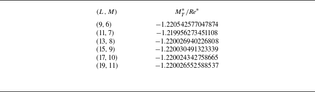
 $(L, \,M)=(19,11)$
is chosen in the following nonlinear calculations. The momentum transport
 $M_T^*$
is used as a nonlinear measure for SVF.
Convergence of the momentum transport
 $M_T^*/{\textit{Re}}^*$
 $(=M_T/{\textit{Re}})$
with respect to the truncation level
 $(L, M)$
for SVF with
 $\alpha =0.1$
and
 $\beta =2.0$
at
 $\tau = 2450$
 $({\textit{Re}}^*=35, \, Q^*=70)$
.

The bifurcation of SVF with various
 $\alpha$
and
 $\beta =2.0$
for
 $\mu =-1$
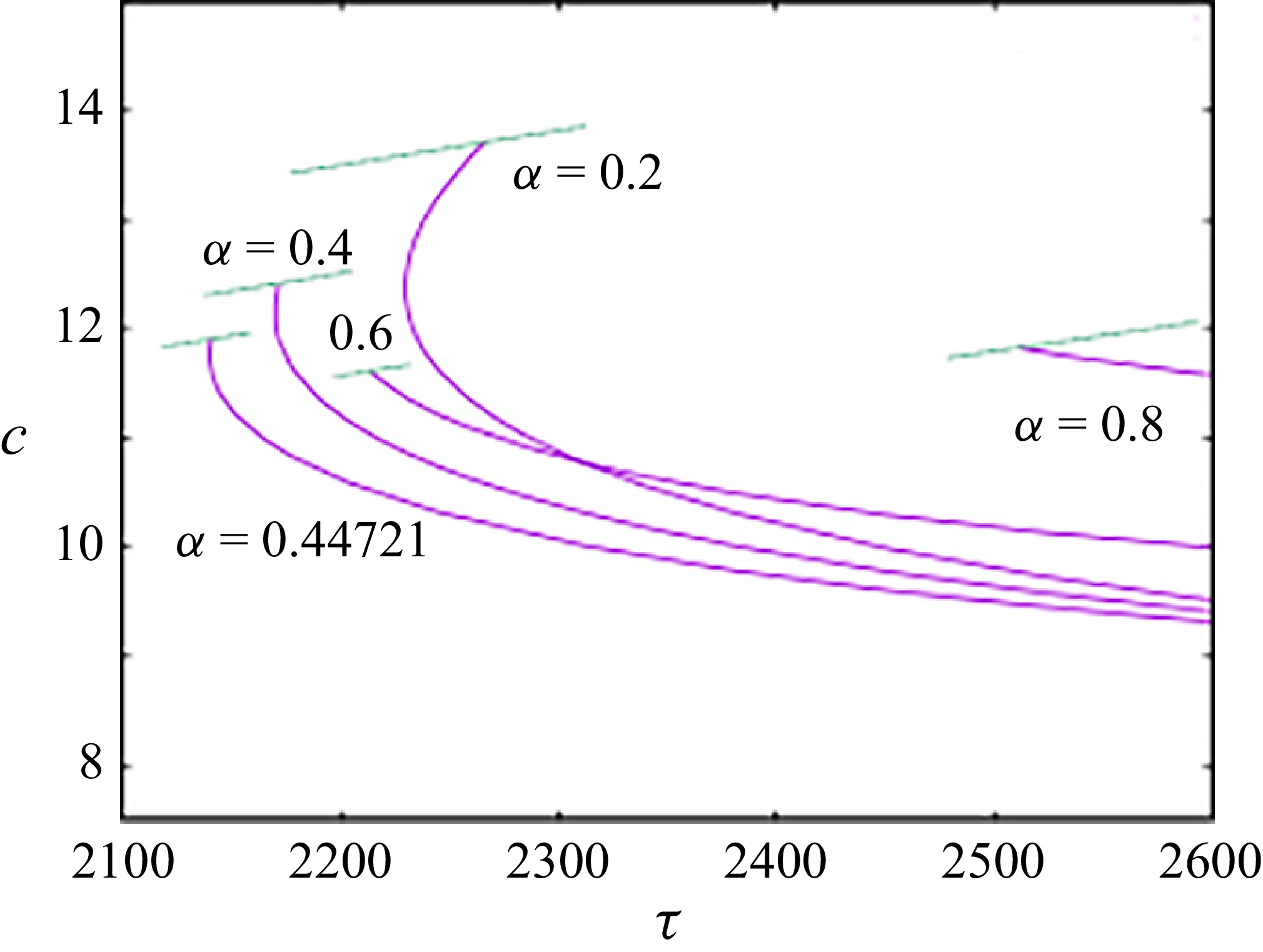
is shown in figure 4. It is seen that the bifurcation of TVF (
 $\alpha =0$
) is subcritical. As
 $\alpha$
is increased from zero, the bifurcation remains subcritical with the bifurcation point below the critical
 $\tau _c(\alpha )$
for TVF. For the SVF branch with
 $\alpha =0.44721$
, the bifurcation takes place at the minimum value of
 $\tau ^{\textit{min}}_c$
. As described above,
 $\tau _c^{\textit{min}}=2140.82$
for
 $\beta =1.821$
. The bifurcation nature of this branch is only slightly subcritical, with a saddle-node point occurring at
 $\tau _{SN}=2140.28$
. As
 $\alpha$
is further increased, the bifurcation point moves to larger values of
 $\tau$
, passes and lies above
 $\tau _c(0)$
for TVF. In accordance with this shift of the bifurcation point to a larger
 $\tau$
, the bifurcation nature changes gradually from subcritical to supercritical as can be seen for the cases of
 $\alpha =0.6$
and
 $0.8$
in figure 4.
The momentum transport
 $M_T^*$
normalised by
 ${\textit{Re}}^*$
as a function of
 $\tau$
for SVF for
 $\mu =-1$
. From left to right on the
 $\tau$
axis:
 $\alpha =$
0.44721, 0.4, 0.6, 0.2, 0.0, 0.8. The axial wavenumber
 $\beta =2.0$
for all
 $\alpha$
, except for the branch of
 $\alpha =0.44721$
where
 $\beta =1.821$
. Since
 $\check {U}^*\equiv 0$
for the basic state,
 $M_T^*/{\textit{Re}}^*=-1$
at the bifurcation point.

At the point of bifurcation from the basic state, the phase speed of SVF satisfies the relation with the imaginary part,
 $\sigma ^I$
, of the eigenvalue
 $\sigma$
of the perturbation determined by the linear stability analysis at the criticality:
 \begin{equation} c= - \sigma ^I/\alpha . \end{equation}
This is checked in figure 5 where the phase speed
 $c$
of SVF and the imaginary part
 $\sigma ^I$
of infinitesimal perturbations near the critical point are plotted. The latter values have previously been plotted in figure 3. It is seen that the phase speed of SVF is always less than that determined by linear analysis. It also appears that the phase speed
 $c$
converges to some constant value for large
 $\tau$
for all
 $\alpha \neq 0$
.
The phase velocity
 $c$
of SVF for
 $\mu =-1$
. The branches of SVF correspond to those in figure 4: from left to right
 $\alpha =$
0.44721, 0.4, 0.6, 0.2, 0.8. The axial wavenumber
 $\beta =2.0$
for all
 $\alpha$
, except for the branch of
 $\alpha =0.44721$
where
 $\beta =1.821$
. The line segments near the bifurcation point indicate
 $\sigma ^I$
for infinitesimal perturbations determined by linear analysis.

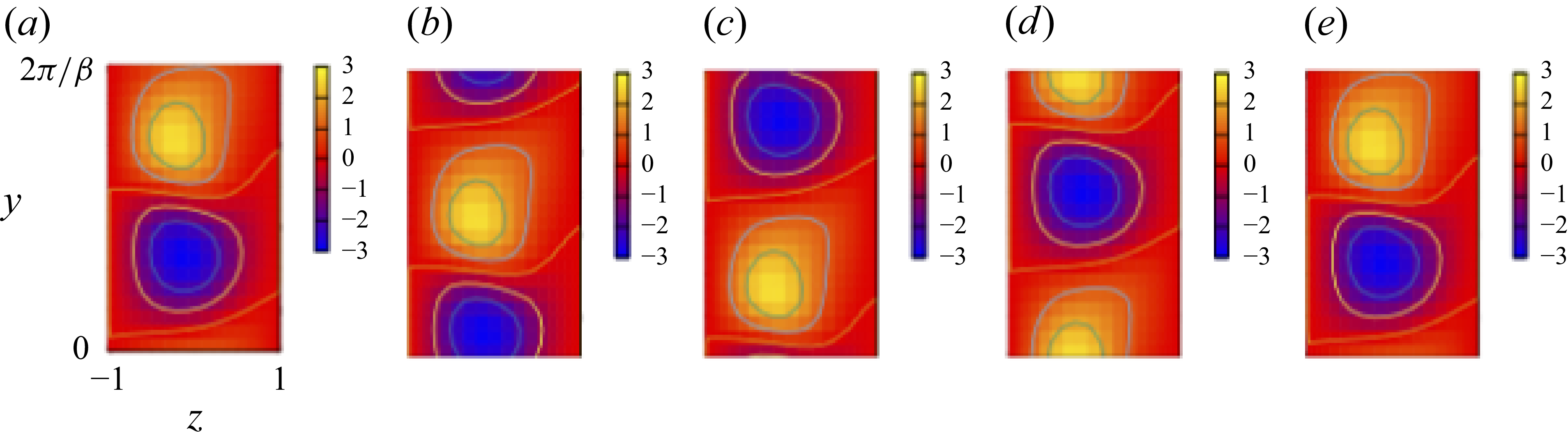
In order to see the flow pattern inside the vortex, we plot
 $\varPsi \equiv \partial _y \phi$
on the
 $(z, \,y$
) cross-section along one wavelength in the
 $x$
direction in figure 6. The vortex centre moves along a direction inclined from the
 $x$
axis. Using
 $\varPsi$
, the disturbance velocity components,
 $\check {u}_y^*$
and
 $\check {u}_z^*$
, in (4.10) are expressed as
 $\check {u}_y^*=\partial _z\varPsi - \partial _x \psi$
and
 $\check {u}_z^*=-\partial _y\varPsi$
. Note that, in contrast to the axisymmetric case (
 $\partial _x\equiv 0$
) of Nagata (Reference Nagata2024), the extra term
 $-\partial _x\psi$
contributes to
 $\check {u}_y^*$
here. This component,
 $\check {u}_y^*$
, is regarded as derived from the stream function
 $\psi$
in the
 $(x,y)$
plane with
 $\check {u}_x^*=\partial _y \psi$
. It can be seen that
 $\varPsi \equiv \partial _y \phi$
is asymmetric about the centre plane
 $z=0$
between the gap. The asymmetry is caused by the inertial effect term with the coefficient
 $Q^*$
in (4.6) which breaks the symmetry in
 $z$
.
The stream function,
 $\varPsi \equiv \partial _y \phi$
, on the
 $(z, y)$
plane at
 $\tau =3000$
for
 $\mu =-1$
. Here
 $\alpha =0.44721$
and
 $\beta =1.821$
: (a)
 $x=0$
; (b)
 $x=0.5\pi /\alpha$
; (c)
 $x=\pi /\alpha$
; (d)
 $x=1.5\pi /\alpha$
; (e)
 $x=2\pi /\alpha$
.

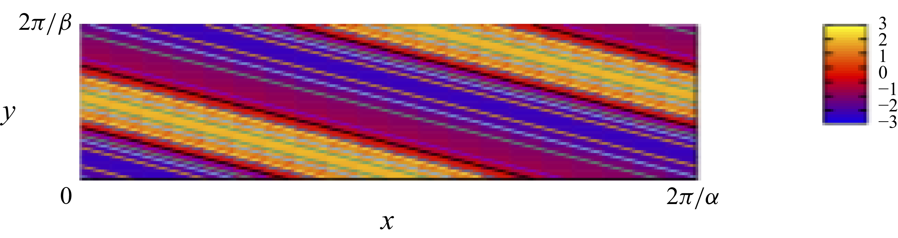
The spiral pattern is shown in terms of the wall-normal component of the disturbance velocity
 $\check {u}_z^*$
on the centre plane
 $z=0$
in figure 7. The pattern in the figure is independent of the direction inclined from the streamwise direction by
 \begin{equation} \gamma = \arctan \Big ({-}\frac {\alpha }{\beta } \Big ). \end{equation}
The inclined pattern is similar to the steady tilted vortex flow in the rotating plane Couette system investigated by Nagata, Song & Wall (Reference Nagata, Song and Wall2021). In contrast, the spiral flow pattern in this study propagates in the azimuthal direction with phase velocity
 $c$
like a barber’s pole. The pattern with the opposite inclination,
 $-\gamma$
, is also possible.
The disturbance velocity component
 $\check {u}_z^*$
on the centre plane
 $z=0$
at
 $\tau =3000$
. The wavenumbers
 $\alpha =0.44721$
and
 $\beta =1.821$
, while
 $\mu =-1$
.

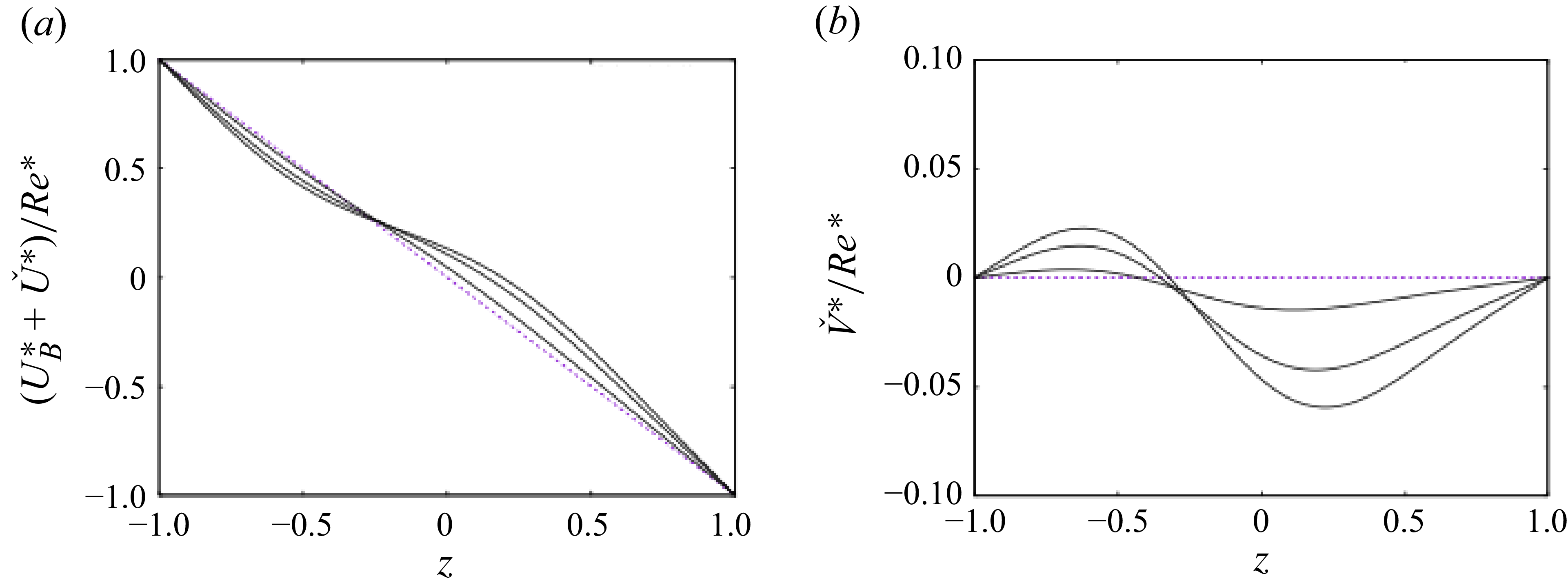
The mean flows normalised by
 ${\textit{Re}}^*$
at
 $\tau = 2200$
, 2600, 3000: (a)
 $({U}_B^* + \check {U}^*)/{\textit{Re}}^*$
and (b)
 $\check {V}^*/{\textit{Re}}^*$
.

The mean flows
 $U_B^* +\check {U}^*$
in the azimuthal direction and
 $\check {V}^*$
in the axial direction, respectively, are plotted in figures 8(a) and 8(b). The asymmetric profiles are due to the symmetry-breaking effect of the inertia terms described above. The asymmetries of the profiles are strengthened as
 $\tau$
is increased.
5. Summary
In this study, we have presented linear and nonlinear analyses of SVFs in the Taylor–Couette system in the limit of a narrow gap between the concentric cylinders. We have applied the system of equations for the axisymmetric case used in Nagata (Reference Nagata2023, Reference Nagata2024) to the non-axisymmetric case. After confirming that the results of our linear stability analysis agreed with those of the study by Krueger et al. (Reference Krueger, Gross and Di Prima1966), branches of nonlinear SVF were sought that bifurcate at the onset of non-axisymmetric instability. We found that a nonlinear SVF inherits the time dependency of the linear eigenmode at the critical point, and travels in the azimuthal direction with phase speed
 $c$
.
Furthermore, we found that the flow pattern and the momentum transport in both the azimuthal and axial directions exhibit an asymmetric distribution across the gap, the asymmetry being due to the effect of the inertia term. This fact clearly distinguishes the Taylor–Couette system in the narrow-gap limit from the plane Couette flow system or the rotating plane Couette flow system, apart from the well-known difference in the linear stability characteristics, namely Taylor–Couette flow becomes unstable to axisymmetric disturbances, whereas plane Couette flow is always stable to infinitesimal disturbances.
For the exact counter-rotating case
 $\mu =-1$
, we found that the bifurcation of the SVF with an axial wavenumber
 $\beta =2.0$
occurs below the critical Taylor number for the axisymmetric case when the azimuthal wavenumber
 $0 \lt \alpha \lessapprox 0.7$
, and above when
 $\alpha \gtrapprox 0.7$
. The bifurcation nature is subcritical for
 $0 \lt \alpha \lessapprox 0.45$
and supercritical for
 $\alpha \gtrsim 0.45$
. This result for
 $\mu =-1$
is consistent with the linear analysis of Krueger et al. (Reference Krueger, Gross and Di Prima1966), who showed that the critical disturbance is axisymmetric (non-axisymmetric) above (below) the critical value
 $\mu =-0.78$
.
We attempt to compare our results with those of the experiments by Snyder (Reference Snyder1970), Andereck et al. (Reference Andereck, Liu and Swinney1986) and Dutcher & Muller (Reference Dutcher and Muller2009). The radius ratios of their experiments are 0.883, 0.912 and 0.959, respectively. In the current study, we showed that the saddle-node point occurs at
 $\tau =2140.2807$
(
 ${\textit{Re}}_{SN}^*=32.713$
) for
 $\alpha =0.44721$
and
 $\beta =1.821=3.642/2$
when
 $\mu =-1$
. Applying the scalings (3.5) to (3.3), we obtain
 \begin{equation} R_i^*= \frac {2\eta }{1-\mu } {\textit{Re}}^*\quad \mbox{and} \quad R_o^*= \frac {2\mu }{1-\mu } {\textit{Re}}^*, \end{equation}
so that we find
 $R_i^*=-R_o^*={\textit{Re}}^*_{SN}=32.713$
for
 $\mu =-1$
. It can be verified that the straight line corresponding to
 $\mu =-1$
drawn in figure 2 of Andereck et al. (Reference Andereck, Liu and Swinney1986), figure 8 of Dutcher & Muller (Reference Dutcher and Muller2009) and figure 18 of Snyder (Reference Snyder1970) intersects the curve for spiral flow detection roughly at
 $R_o\ ( \equiv ({\omega _o r_o(r_o-r_i)}/{\nu }))=-250$
,
 ${\textit{Re}}_o\ (\equiv ({\omega _o r_o(r_o-r_i)}/{\nu}))=-300$
and
 $R_2^2{ \varOmega _2}/\nu \ (\equiv ({r_o^2\omega _o }/{\nu }))=-9\times 10^3$
, respectively, where variables
 $\omega _o$
,
 $r_i$
,
 $r_o$
and
 $\nu$
inside the parentheses are those used in the present study. These experimental values are scaled by
 $\sqrt {1-\eta }$
with the radius ratio
 $\eta$
provided above to yield
 $R_o^* = \sqrt {1-\eta }R_0 = - 42.76$
,
 $ {\textit{Re}}_o^* = \sqrt {1-\eta }{\textit{Re}}_0 = - 44.49$
and
 $\sqrt {1-\eta }R_2 {\textrm d} { \varOmega _2}/\nu = - 37.36$
, respectively, after changing the length scale from full, (
 $r_o-r_i$
), to the half-gap width. These values should be compared with our theoretical value,
 $R_o^*=-32.713$
.
The existence region of SVF is next examined for a wide range of values of
 $\mu$
in the
 $(R_o^*, \,R_i^*)$
space. In figure 9(a), the red dotted and the red solid curves are the linear neutral curve and the trace of the saddle-node points, respectively, for SVF with
 $\alpha =0.5$
. Also shown in the figure by the black dotted and the black solid curves are the linear neutral curve and the trace of the saddle-node points, respectively, for axisymmetric TVF (
 $\alpha =0$
), which duplicates the data of figure 10 of Nagata (Reference Nagata2024). Figure 9(b) compares the current theoretical results with the experimental observations in the scaled
 $(Ro^*, \,Ri^*)$
space, where the green, blue and pink curves, reproduced from figure 2 of Andereck et al. (Reference Andereck, Liu and Swinney1986), figure 8 of Dutcher & Muller (Reference Dutcher and Muller2009) and figure 18 of Snyder (Reference Snyder1970), respectively, show the boundary of the existence region of SVF. Above the upper branches of the bounding curves these studies observed interpenetrating spirals for Andereck et al. (Reference Andereck, Liu and Swinney1986) and Dutcher & Muller (Reference Dutcher and Muller2009) or mixed spiral and Taylor cells for Snyder (Reference Snyder1970), while below the lower branches they all observed circular Couette flow. Along each of these lower branches both the axial and azimuthal wavenumbers change. Here, we approximate the bounding lower branches by an envelope, connecting the saddle-node points for the axial wavenumber restricted to
 $\beta =2.0$
. The black thin lines in figure 9(b) correspond to this envelope. Although the value of
 $\alpha$
should change continuously along the envelope, in principle, only two discrete values of
 $\alpha =0.44721$
for
 $R_o^*\in [-38, \, -32.71]$
and
 $\alpha =0.5$
for
 $R_o^*\in [-50, \, -38]$
are used to draw two line segments in the figure. The extension of the envelope to increasing
 $R_o^*$
seems to indicate that the
 $\alpha$
value along the envelope decreases to zero, thus corresponding to the axisymmetric case at
 $R_o^*\approx -20.6$
, while extension to decreasing values of
 $R_o^*$
finds that
 $\alpha$
further increases to
 $\alpha =0.6$
for
 $R_o^*\in [-70, \, -50]$
and to
 $\alpha =0.7$
for
 $R_o^*\in [-80, \, -70]$
. The theoretical findings above are in reasonable agreement with experimental observations of SVF, considering, for example, that the radius ratios are not very close to 1, the finiteness of the aspect ratio (the ratio of height to radius) of the experimental set-ups, uncertainty in evaluation of the kinematic viscosity and so on.
(a) The existence boundaries of TVF and SVF in the
 $(R_o^*,\,R_i^*)$
space. The black dotted and solid curves connect the linear neutral points and the saddle-node points, respectively, for axisymmetric TVF, while the red dotted and solid curves connect the linear neutral points and the saddle-node points, respectively, for SVF with
 $\alpha =0.5$
. (b) Comparison with experimental observations of the existence region of SVF by Andereck et al. (Reference Andereck, Liu and Swinney1986) (green), Dutcher & Muller (Reference Dutcher and Muller2009) (blue) and Snyder (Reference Snyder1970) (pink). The black thin line segments approximate the envelope for the saddle-node points for
 $\beta =2.0$
. The black dotted curve corresponds to the neutral curve for TVF (
 $\alpha =0$
). The dotted straight lines with colour (green, blue, pink and black) correspond to the lines given by
 $R_i^*= ({\eta }/{\mu }) R_o^*$
with
 $\mu =-1$
for Snyder (Reference Snyder1970), Andereck et al. (Reference Andereck, Liu and Swinney1986), Dutcher & Muller (Reference Dutcher and Muller2009) and the current theoretical study, respectively. The points of detection of SVF for
 $\mu =-1$
in these experiments are on these dotted straight lines and indicated by triangles.

The lower boundary for the existence of SVF on the scaled Reynolds number space,
 $(R_o^*,R_i^*) \equiv (\sqrt {1-\eta }R_o \, , \, \sqrt {1-\eta }R_i)$
, is determined by the saddle-node point of the subcritical SVF branch, not by the linear critical point as was determined by Langford et al. (Reference Langford, Tagg, Kostelich, Swinney and Golubitsky1988) in linear analysis of primary instabilities and bi-criticality in finite-gap cases.
Taken together with the results of the previous investigations by the author (Nagata Reference Nagata2023, Reference Nagata2024) for the axisymmetric case, the present investigation on linear and nonlinear analyses for the non-axisymmetric case provides a basis for studying further transitions from axisymmetric TVF and non-axisymmetric SVF in the narrow-gap limit of the Taylor–Couette system, beyond the weakly nonlinear analyses by Demay et al. (Reference Demay, Looss and Laure1992a ), Demay et al. (Reference Demay, Iooss and Laure1992b ), Chossat et al. (Reference Chossat and Iooss1994) and Itoh (Reference Itoh1996) described in § 1.
Declaration of interests
The author reports no conflict of interest.
Appendix A
The nonlinear terms
 $\hat {\boldsymbol k}\boldsymbol{\cdot }\boldsymbol{\nabla }\times \boldsymbol{\nabla }\times [\check {\boldsymbol u}^*\boldsymbol{\cdot }\check { {\boldsymbol u}}^* ]$
and
 $\hat {\boldsymbol k}\boldsymbol{\cdot }\boldsymbol{\nabla }\times [\check {\boldsymbol u}^*\boldsymbol{\cdot }{ {\check {\boldsymbol u}}^*}$
, which appear in (3.12) and (3.13), respectively, can be found in an explicit form in Masuda, Fukuda & Nagata (Reference Masuda, Fukuda and Nagata2008). In there,
 $\phi$
and
 $\psi$
and all of their partial derivatives with respect to
 $x$
,
 $y$
and
 $z$
are of
 $\mathcal{O}(1)$
, whereas the nonlinear terms in (4.6) and (4.7) excluding those terms with an unnecessary number of
 $x^*$
derivatives, such as
 $\partial _x\acute \partial _x$
and
 $(\partial _x+\acute \partial _x)^2$
, are of
 $\mathcal{O}(1-\eta )$
. After taking into account of the fact that
 $\phi \sim \mathcal{O}(1)$
and
 $\psi \sim \mathcal{O}(1/\sqrt {1-\eta })$
, we express
 $\hat {\boldsymbol k}\boldsymbol{\cdot }\boldsymbol{\nabla }\times \boldsymbol{\nabla }\times [ {\check {\boldsymbol u}}^*\boldsymbol{\cdot }{ \check {\boldsymbol u}^*}] \sim \mathcal{O}(1)$
and
 $\hat {\boldsymbol k}\boldsymbol{\cdot }\boldsymbol{\nabla }\times [\check {\boldsymbol u}^*\boldsymbol{\cdot }{ \check {\boldsymbol u}^*}] \sim \mathcal{O}(1/\sqrt {1-\eta })$
explicitly as follows:
 \begin{align} \hat {\boldsymbol k}\boldsymbol{\cdot }\boldsymbol{\nabla }\times \boldsymbol{\nabla }\times [\check {\boldsymbol u}^*\boldsymbol{\cdot }{ \check {\boldsymbol u}^*}] &= \Big ( \partial _y \acute {\partial }_y \big(2\partial _y\acute \partial _y +\acute \partial ^2_{yy} \big) -\partial ^2_{yy}\acute \partial ^2_{yy} \Big ) \phi _z \acute \phi _{zz} \nonumber \\&\quad+ \big(\partial _y + \acute \partial \big)^2 \partial ^2_{yy} \big(\partial _y\acute \partial _y - \acute \partial ^2_{yy} \big) \phi \acute \phi _{z} \nonumber \\&\quad- \partial ^2_{yy}\big(\partial _y\acute \partial _y+ \acute \partial ^2_{yy}\big)\phi \acute \phi _{zzz} \nonumber \\&\quad+ \big( \partial _x\acute \partial _y - \partial _y\acute \partial _x \big) \big(2\partial _y\acute \partial _y+\partial ^2_{yy} \big) \phi _{zz} \acute \psi \nonumber \\&\quad+ 2\big( \partial _x\acute \partial _y - \partial _y\acute \partial _x \big)\partial _y\acute \partial _y \phi _z \acute \psi _z \nonumber \\&\quad+ \big(\partial _y+\acute \partial _y\big)^2 \partial ^2_{yy}\big( \partial _x\acute \partial _y - \partial _y\acute \partial _x \big) \phi \acute \psi \nonumber \\&\quad- \big(\partial _y+\acute \partial _y \big)^2 \partial ^2_{yy}\big(\partial _x\acute \partial _y-\partial _y \acute \partial _x\big) \phi \acute \psi _{zz} \nonumber \\&\quad- 2\big(\partial _x\acute \partial _y - \partial _y\acute \partial _x\big)^2 \psi \acute \psi _{z} \end{align}
and
 \begin{align} \hat {\boldsymbol k}\boldsymbol{\cdot }\boldsymbol{\nabla }\times [\check {\boldsymbol u}^*\boldsymbol{\cdot }{ \check {\boldsymbol u}^*}] &= -\, \partial ^2_{yy} \phi \acute \phi _{zz} \nonumber \\&\quad- \acute \partial ^2_{yy} \partial _y \big(\partial _y + \acute \partial _y\big)\phi _{z} \acute \psi \nonumber \\&\quad+ \partial ^2_{yy} \acute \partial y \big(\partial _y + \acute \partial _y\big) \phi \acute \psi _z \nonumber \\&\quad- \partial ^2_{yy} \big( \partial _x\acute \partial _y - \partial _y\acute \partial _x\big) \psi \acute \psi , \end{align}
where, following Masuda et al. (Reference Masuda, Fukuda and Nagata2008), the differential operators with a prime indicate the operation on
 $\phi$
or
 $\psi$
with a prime on the same line, and similarly, the differential operators without a prime indicate the operation on
 $\phi$
or
 $\psi$
without a prime on the line.