INTRODUCTION
Soft bottom macroinvertebrates are recognized as useful indicators of ecological status of marine coastal systems (Rosenberg et al., Reference Rosenberg, Nilsson and Diaz2001; Junoy et al., Reference Junoy, Castellanos, Viéitez, de la Huz and Lastra2005; Calabretta & Oviatt, Reference Calabretta and Oviatt2008) and are widely used to detect the ecological quality of water bodies (Borja et al., Reference Borja, Franco and Perez2000; Perus et al., Reference Perus, Bonsdorff, Bäck, Lax, Villnäs and Westberg2007; Teixeira et al., Reference Teixeira, Magalhães Neto, Patrício, Veríssimo, Pinto, Salas and Marques2009; Carvalho et al., Reference Carvalho, Barata, Pereira, Pousão-Ferreira, Cancela da Fonseca and Gaspar2010). Macrobenthos responds relatively rapidly to anthropogenic and natural stress and changes in abundance, biomass and species composition in assemblages are considered related to the degree of pollution or to other kinds of disturbance (Dauer, Reference Dauer1993; Bonsdorff & Pearson, Reference Bonsdorff and Pearson1999; Gray et al., Reference Gray, Wu and Or2002; Karlson et al., Reference Karlson, Rosenberg and Bondsorff2002). With regards to macrobenthic communities, both univariate measures, such as abundance, diversity or biomass, and multivariate methods are used to assess the state of the marine environment (Harkantra & Rodrigues, Reference Harkantra and Rodrigues2004; Marin-Guirao et al., Reference Marin-Guirao, Cesar, Marin, Lloret and Vita2005; Rosenberg & Nilsson, Reference Rosenberg and Nilsson2005).
When using biotic indicators for environmental impact assessment of coastal areas, the spatial scale considered is extremely important (Chapman et al., Reference Chapman, Underwood and Skilleter1995; Hewitt et al., Reference Hewitt, Thrush and Cummings2001) in order to discriminate between patterns resulting from natural and anthropogenic pressures (Zmarzly et al., Reference Zmarzly, Stebbins, Pasko, Dugga and Barwick1994; Underwood, Reference Underwood2000). Actually, the response of assemblages to gradients related to a point-source of pollution may be not independent from wider gradients of disturbance that act on the same areas. Moreover, the amplitude of changes in the structure of assemblages following a disturbance event can vary according to the environmental characteristics of a determinate area (Raimondi & Reed, Reference Raimondi, Reed, Schmitt and Osenberg1996), increasing the bias when analysing the results of monitoring and environmental impact assessment studies. In this context, an important goal for ecologists is to discriminate between effects related to disturbances acting at different spatial scales.
The aim of the present study was to evaluate the interactions between different gradients of disturbance acting on different spatial scales to determine the structure of soft-bottom macroinvertebrate assemblages. Two different spatial scales were considered: a small-scale gradient, related to a growing distance from the outfall, and a large-scale gradient, related to the level of pollution within a large bay in western Italy. The following hypotheses were tested: (i) the structure of benthic assemblages does not change along a gradient of distance from a point-source of pollution; and (ii) the overall level of anthropogenic pressure of a sampling area does not influence the structure of benthic assemblages along a gradient of distance from a point-source of pollution.
MATERIALS AND METHODS
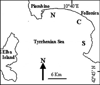
The study was carried out in the Gulf of Follonica, a 30 km wide bay, located on the western coast of Italy, in the north-western Mediterranean Sea (Figure 1). Several small rivers that flow into the bay transport different kinds of wastewater from adjacent industrial, urban and agricultural areas and represent point sources of pollution. The main human activities are sited in the northern zone, contributing to create a gradient of disturbance from a higher polluted area in the northern part of the bay subjected to organic, chemical and thermal pollution (Lardicci et al., Reference Lardicci, Rossi and Maltagliati1999; Bedini et al., in press) to a less polluted southern area.
Map of the study area. N, C and S indicate northern area, central area and southern area respectively.

Three different areas were selected within the bay from north to south (northern, N; central, C; and southern, S). In each area, three different distances from river mouths were considered: near (n, <20 m), intermediate (i, 50 m) and far (f, 100 m). Two periods (spring–summer (SS) and autumn–winter (AW)) were considered within one-year and two dates were sampled in each period. At each distance and for each sampling date, 5 replicates samples were collected. The sampling depth ranged between 4 and 8 m; the seabed sediments in the three studied areas were primarily sand (ranging between 88.71% and 99.18%) with a small percentage of mud (between 0.67% and 3.05%).
Sediments were collected by SCUBA diving, using a Plexiglas corer 30 cm long and 10 cm wide (0.00785 m2) (Gambi et al., Reference Gambi, Conti and Bremec1998; Ysebaert & Herman, Reference Ysebaert and Herman2002). Samples were washed through 0.5 mm mesh sieve and fixed in formalin–seawater (6%) before sorting and taxonomic identification of organisms at the laboratory. Whenever possible taxa were identified at species level and the abundance of each taxon was expressed as number of individuals. The abundances of the main classes/phyla were also calculated by summing the abundances of all taxa belonging to each phylum or class.
Species composition and abundance were analysed by permutational analysis of variances (PERMANOVA; Anderson, Reference Anderson2001). A 4-way model was used with Area (N versus C versus S), Distance (n versus i versus f) and Period (SS versus AW) as fixed and crossed factors and Date (2 levels) as random factor nested in Period. The Bray–Curtis similarity index was calculated using untransformed data. The PAIRWISE test was used to discriminate among levels of significant factors. The similarity of percentages (SIMPER) test was used to establish which taxa mostly contributed to the dissimilarity between groups (Clarke, Reference Clarke1993).
Alpha diversity was evaluated as species richness and Shannon–Weaver index, while beta diversity within each area was estimated as the participation of the differences between samples to alpha diversity (Gray, Reference Gray2000): βs = NC / λ, where NC = the species richness in the condition c, λ = the average sample species richness in the condition c.
The total number of organisms per plot, the total number of species, values of Shannon–Weaver index and the abundance of the main taxa, were analysed by univariate analyses of variance (ANOVA; Underwood, Reference Underwood1997) using the same factors and levels considered in the multivariate analyses. Homogeneity of variance was tested by Cochran's C test. The Student–Newman–Keuls (SNK) test was used to discriminate among levels of significant factors.
Taxa were divided in ecological groups and the AZTI Marine Biotic Index's biotic coefficient was calculated for each studied condition in agreement with Borja et al. (Reference Borja, Franco and Perez2000): BC =.{(0 × %GI) + (1.5 × %GII) + (3 × %GIII) + (4.5 × % GIV) + (6 × GV)}/100, where GI are species of normal community, GII are species of impoverished community, GIII are species of unbalanced community, GIV and GV are species of polluted community, and GVI are species of heavy polluted community.
RESULTS
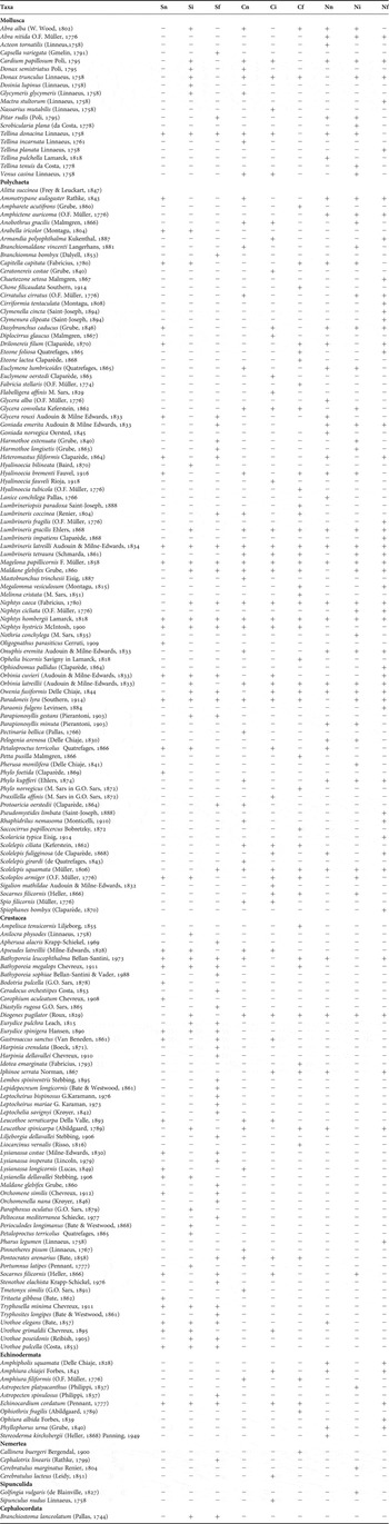
A total of 187 taxa were found, among them 94 Polychaeta, 57 Crustacea, 19 Mollusca, 10 Echinodermata, 2 Sipunculida, 1 Cephalocordata and 4 Nemertea (Table 1). Crustacea, Polychaeta and Mollusca were the most abundant groups, whereas Echinodermata, Cephalocordata, Sipunculida and Nemertea presented low abundances.
List of taxa. n, near; i, intermediate; f, far; N, northern area; C, central area; S, southern area.

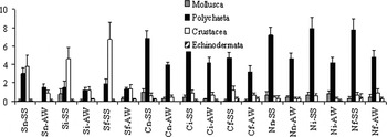
Polychaeta were mostly abundant in N and C areas, while Crustacea were more abundant in area S. Moreover, Crustacea abundance increased from (n) to (f) sites. Both Polychaeta and Crustacea decreased in the AW period (Figure 2).
Main taxa abundances in relation to area (N versus C versus S), distance from river mouths (n versus i versus f) and period (SS versus AW) (see text for definitions of abbreviations).

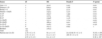
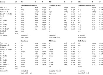
PERMANOVAs detected a significant interaction between Area and Distance. The PAIRWISE test showed that differences among distance were not significant in N; in C, (n) and (i) were different from (f), while, in S, (n) was different from the remaining. Site S was significantly different from the other areas in (n) and (i); in (f), areas were different from each other. The interaction between Period and Area was also significant; however, the PAIRWISE test showed that differences between periods were significant in all areas and N and C differed from S in both periods (Table 2).
Results of permutational analysis of variance. n, near; i, intermediate; f, far; N, northern area; C, central area; S, southern area.

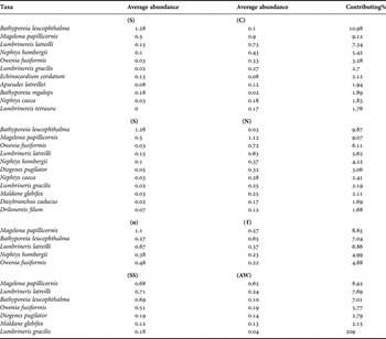
The SIMPER test showed that taxa mostly contributing to separate areas were the crustaceans Bathyporeia leucophthalma and B. megalops, more abundant in area S, and the polychaetes Lumbrineris latreilli, Magelona papillicornis, Nephtys hombergii, Owenia fusiformis and Maldane glebifex, more abundant in N and C areas (Table 3). Along a gradient of distance from the coast, Bathyporeia leucophthalma was more abundant in (f), while Lumbrineris latreilli, Magelona papillicornis, Nephtys hombergii and Owenia fusiformis were more abundant in (n) (Table 4). Differences between periods were mostly related to changes in abundance of the main taxa; in particular Lumbrineris latreilli, Bathyporeia leucophthalma and Owenia fusiformis decreased in the AW period (Table 3).
Results of similarity of percentages test showing taxa that mostly contributed to separate assemblages between areas (S versus C and S versus N), distance (n versus f) and periods (SS versus AW) (see text for definitions of abbreviations).

Results of analyses of variance.

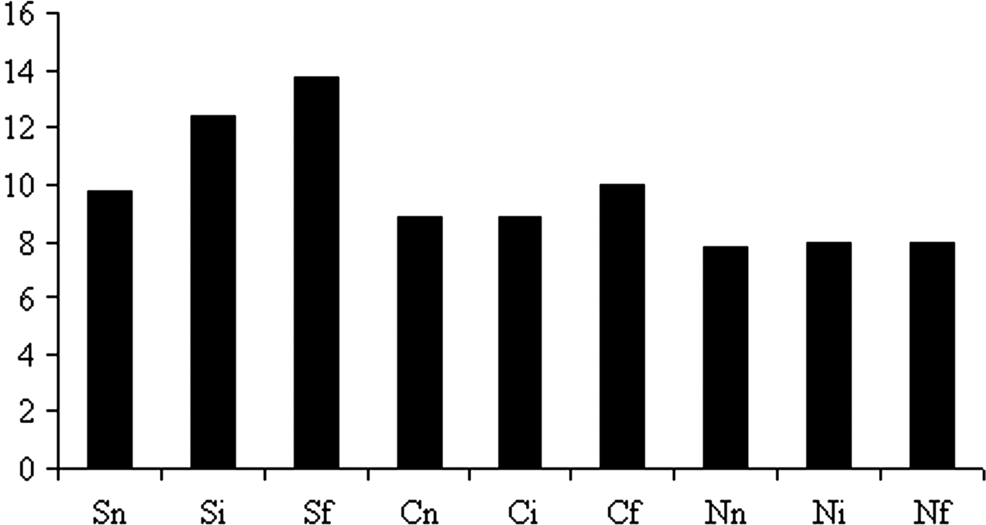
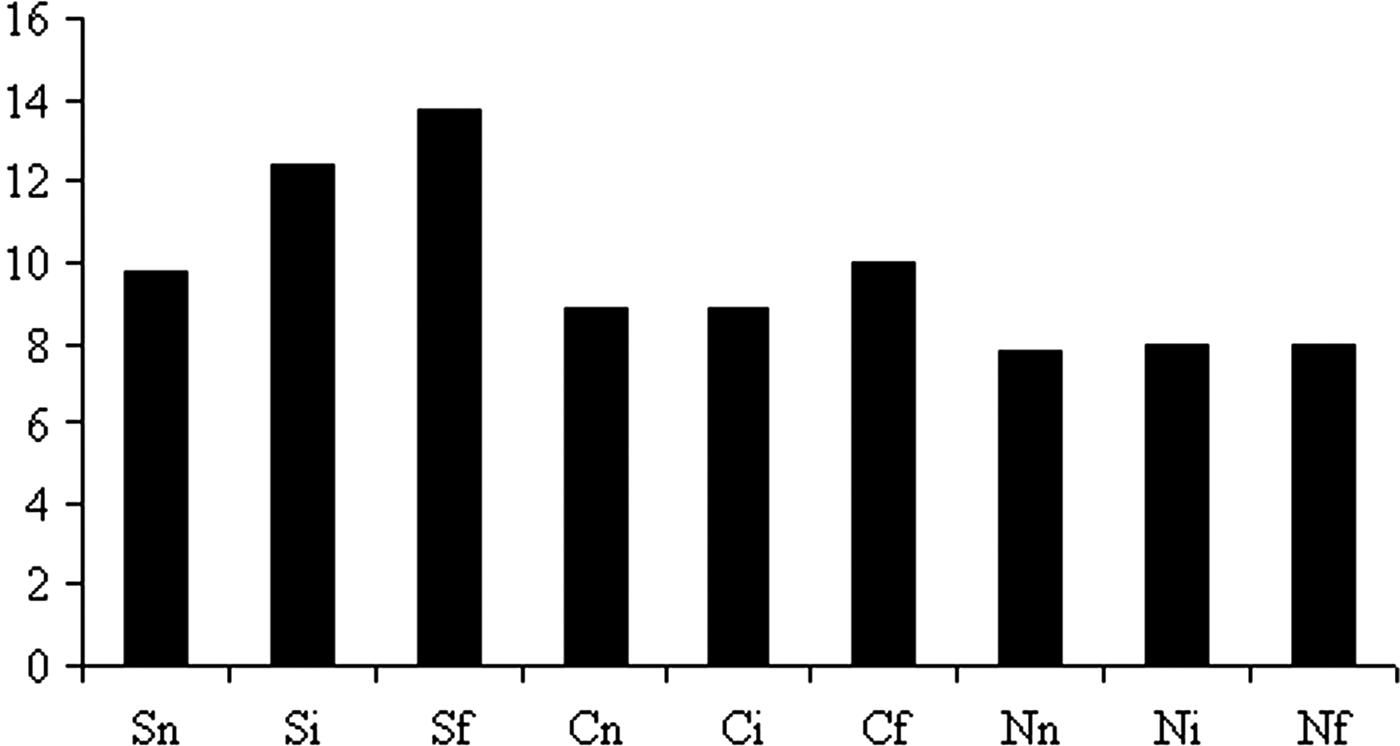
The total richness was similar in the three areas (91, 91 and 87 in S, C and N respectively), while beta diversity showed patterns related to both area and distance. In area S, beta diversity decreased along the pollution gradient; this pattern was less evident in area C and completely missing in area N (Figure 3). Mean values decreased from areas S to N.
Values of beta diversity in relation to area (N versus C versus S) and distance from river mouths (n versus i versus f) (see text for definitions of abbreviations).
The ANOVA detected a significant interaction between Area and Distance for the total number of organisms per plot, the total number of species per plot and the abundance of Polychaeta. For all these variables, the SNK test showed that differences among distances were not significant in the area (N); in the area (C), (n) and (i) were different from (f), while in the area (S), (n) was different from the other distances. (S) was different from the other areas in (n) and (i) while, in (f), areas were different from each other. Values of the Shannon–Weaver index were lower in (S) than in the other areas. The abundance of Crustacea was higher in (f) than in the other distances, while no significant effects were detected for the abundance of Mollusca (Table 4).
Values of biotic coefficient decrease from n to f in S area, while no evident patterns were detected in C and N areas (Table 5).
Percentage of ecological groups in the studied conditions and values of biotic coefficient. n, near; i, intermediate; f, far; N, northern area; C, central area; S, southern area.

DISCUSSION
The patterns of variability of macroinvertebrate assemblages along gradients of disturbance were found to be influenced by the ecological conditions of the studied areas. Changes in the structure of assemblages related to the distance from sewage sources differed in relation to large-scale gradients of pollution and they were not evident in the higher polluted area of the studied bay. Differences among conditions were evident independently from seasonal changes.
The lack of similar studies does not allow comparison of these results with patterns already reported. However, it is known that disturbance is likely to interact with other physical and biological processes creating heterogeneous patterns of stress that are superimposed upon existing spatial variability (Raimondi & Reed, Reference Raimondi, Reed, Schmitt and Osenberg1996). Thus, the concurrent presence of impacts acting at different spatial scales may prevent the detection of differences between controls and impact sites without appropriate sampling designs. Results of the present study agree with previous investigations highlighting the importance of spatial scale of impact to determine the choice of sampling procedures (Hewitt et al., Reference Hewitt, Thrush and Cummings2001). In fact, the size of the monitored impact site, the spatial variability within the sites and the distance of control sites are determined by the spatial scale of impact. Appropriate sampling designs taking into account multiple spatial scales are needed to detect large-scale impact, especially when different gradients are superimposed in the same area.
The results confirm the value of macroinvertebrate assemblages as indicator of anthropogenic disturbance (Marin-Guirao et al., Reference Marin-Guirao, Cesar, Marin, Lloret and Vita2005; Teixeira et al., Reference Teixeira, Magalhães Neto, Patrício, Veríssimo, Pinto, Salas and Marques2009). Changes of environmental conditions throughout the studied bay were highlighted by changes in the structure of benthic assemblages; in particular, Polychaeta increased while Crustacea decreased in more polluted areas. Polychaeta are known as being sensitive to environmental gradients (Gambi & Giangrande, Reference Gambi and Giangrande1986) and many species are considered tolerant to pollution and they are widely used as indicators of water quality (Chou et al., Reference Chou, Yu and Loh2004; Rosenberg & Nilsson, Reference Rosenberg and Nilsson2005). However, in the present study, species considered characteristic of unpolluted areas, such as Magelona papillicornis, Owenia fusiformis and Maldane glebifex (Borja et al., Reference Borja, Franco and Perez2000), were abundant in disturbed sites; moreover, several species showed severe temporal fluctuations. The use of single species to detect pollution is a debated issue, as the same species may show different ecological responses in different geographical regions or at different times (Bedini et al., Reference Bedini, Canali and Cappagli2003; Dean, Reference Dean2008). Moreover, populations may adapt to peculiar environmental conditions through short-term selection mechanisms, showing unpredictable behaviours (Cognetti, Reference Cognetti1978; Cognetti & Maltagliati, Reference Cognetti and Maltagliati2000). On the contrary, results of the present study underlined the suitability of multivariate analysis of the whole community and univariate analyses of higher taxa to detect environmental changes.
The different aspects of biodiversity used in the present study showed contrasting patterns. Alpha diversity appeared not correlated with the level of disturbance, as values of total species richness were similar among the studied conditions and the used biodiversity descriptors did not show a common trend; on the contrary, changes of beta diversity followed the gradients of pollution. Alpha diversity is widely recognized as a valuable indicator of ecological quality of soft-bottom marine habitat (Gray, Reference Gray1997; Godínez-Domínguez et al., Reference Godínez-Domínguez, Freire, Franco-Gordo and González-Sansón2009), while the importance of beta diversity has been less considered (Ellingsen, Reference Ellingsen2001). The decrease of beta diversity could represent a serious ecological problem, leading to an increase of biotic homogenization (McKinney & Lockwood, Reference McKinney and Lockwood1999). This phenomenon, due to proliferation of opportunistic species, represents a main biotic impoverishment of natural systems, with severe consequences for the functioning of ecosystems (Olden et al., Reference Olden, Poff, Douglas, Douglas and Fausch2004), and it has been mostly attributed to organic and chemical pollution derived from industrial and urban sewage effluents (Valiela et al., Reference Valiela, Foreman, LaMontagne, Hersh, Costa, Peckol, DeMeo-Anderson, d'Avanzo, Babione, Sham, Brawley and Lajtha1992). Results of the present investigation showed that beta diversity may be a useful tool to detect gradients of disturbance and it should be concurrently used together with alpha diversity in monitoring survey and impact evaluation studies.
Temporal dynamics related to seasonal patterns has been widely described for soft-bottom assemblages (Doğan et al., Reference Doğan, Çinar, Önen, Ergen and Katağan2005; Lu & Wu, Reference Lu and Wu2007; Godínez-Domínguez et al., Reference Godínez-Domínguez, Freire, Franco-Gordo and González-Sansón2009). In the present study, differences in the structure of assemblages were more due to changes in abundance of the main taxa than to modifications in species composition. Probably, different environmental conditions mostly related to seasonal differences in river flows could contribute to these dynamics together with the life cycles of organisms (Bachelet et al., Reference Bachelet, de Montaudouin, Auby and Labourg2000). In fact, river flows may strongly influence the structure of benthic assemblages also modifying patterns of seasonal dynamics (Denisenko, Reference Denisenko2009).
Results showed that different gradients of disturbance acting in the same area at different spatial scales may interact, making difficult the interpretation of patterns of variability. This finding underlines the importance of appropriate sampling designs in impact evaluation surveys, in order to separate different sources of variability of the systems. Results also confirm the suitability of the concurrent use of multivariate and univariate techniques to detect consequences of disturbance in ecological studies (Rosenberg & Nilsson, Reference Rosenberg and Nilsson2005; Terlizzi et al., Reference Terlizzi, Benedetti-Cecchi, Beviliacqua, Fraschetti, Guidetti and Anderson2005; Balata et al., Reference Balata, Piazzi and Cinelli2007). In fact, different approaches may highlight different effects of environmental alterations, allowing a more complete evaluation of the ecological quality of coastal habitats, especially when more disturbances concurrently act on the same area.
ACKNOWLEDGEMENTS
This research was supported by ‘Assessorato all'Ambiente della Provincia di Livorno’, ‘Comune di Piombino’ and ‘Piombino Port Authority’.