Introduction
Animal diversity increased from a single, ancestral species that lived at some point in Neoproterozoic time (1000 to 541 Ma) to the many millions of species that inhabit Earth today. In his Homage to Santa Rosalia, Hutchinson (Reference Hutchinson1959) asked why contemporary animal diversity is so high. As an answer, he proposed that resource availability regulates taxonomic diversity and that taxonomic diversity accumulates via functional differentiation (Hutchinson Reference Hutchinson1959), implying that diversity typically sits at or near the carrying capacity imposed by available resources (Rabosky and Hurlbert Reference Rabosky and Hurlbert2015). This interpretation has not been accepted universally. Others have instead proposed that diversity remains far from any limit and that most ecological systems are open to invasion and species accumulation (Stanley Reference Stanley2007; Harmon and Harrison Reference Harmon and Harrison2015). Under the former scenario, temporal and spatial variation in taxonomic and functional diversity should reflect resource availability (Rabosky and Hurlbert Reference Rabosky and Hurlbert2015). Under the latter, the two should be largely decoupled. More than half a century after Hutchinson posed them, the questions of whether animal diversity is near carrying capacity and regulated by resource availability remain unresolved. Furthermore, the extent to which diversity has existed near carrying capacity across evolutionary time remains debated (e.g., Sepkoski Reference Sepkoski1984; Stanley Reference Stanley2007).
Of the resources potentially limiting to diversity, none has received more attention than primary productivity (i.e., energy availability; Clarke and Gaston Reference Clarke and Gaston2006). Underlying the hypothesized energy–diversity relationship rests a variety of potential processes that can be grouped broadly into energy budget and energy adaptation mechanisms. In the energy budget model, energy is an allocated resource that can be translated into work and mass. Many hypotheses for energy–diversity relationships assume a positive association between primary productivity and taxonomic diversity (Rosenzweig and Abramsky Reference Rosenzweig and Abramsky1993; McClain and Schlacher Reference McClain and Schlacher2015). Two such hypotheses, the “more individuals” and “one more trophic level” hypotheses, have received the most attention in the literature. More energy can support more individuals, buffering against local extinctions, and thus can support a larger number of species (“species-energy” or more individuals hypothesis; Wright Reference Wright1983; Wright et al. Reference Wright, Currie and Maurer1993; Srivastava and Lawton Reference Srivastava and Lawton1998). The “one more trophic level” hypothesis proposes that increased growth and reproduction of consumers enabled by increased energy availability allows the ecosystem to support both more trophic levels and a greater diversity of predators at higher trophic levels (Abrams Reference Abrams1993; Moen and Collins Reference Moen and Collins1996; Post Reference Post2002a). Under the energy adaptation model, species are adapted to specific energy regimes. In other words, there are “high-energy” and “low-energy” species. High-energy species, those with greater metabolic demands, cannot persist in low-energy environments. Low-energy species thrive in low-energy environments but also occur in high-energy environments, because these species can persist on the energy remnants not captured by high-energy species. Indeed marine communities at low productivities appear to be nested subsets of communities at high productivities (Brault et al. Reference Brault, Stuart, Wagstaff, McClain, Allen and Rex2013; McClain et al. Reference McClain, Barry, Eernisse, Horton, Judge, Kakui, Mah and Waren2016). Prior research has also demonstrated that the presence and dominance of functional types, as measured by such traits as body size and life history, vary with energy availability (e.g., Blackburn and Gaston Reference Blackburn and Gaston1996; Aava Reference Aava2001; Terribile et al. Reference Terribile, Olalla-Tarraga, Diniz-Filho and Rodriguez2009; Marshall et al. Reference Marshall, Krug, Kupriyanova, Byrne and Emlet2012; McClain et al. Reference McClain, Gullet, Jackson-Ricketts and Unmack2012a, Reference McClain, Filler and Auld2014), suggesting a link between energetic demand and specific species’ traits. In addition, traits that affect energy acquisition, such as feeding types or trophic niches, should provide another potential connection between food availability and taxonomic or functional diversity in energy diversity gradients (Schoener Reference Schoener1976; DeAngelis Reference DeAngelis1994; Evans et al. Reference Evans, Warren and Gaston1999, Reference Evans, Greenwood and Gaston2005). This adaptive view is similar to the ideas of Tilman (Reference Tilman1982), in which species are adapted to a particular resource level or resource ratios. Overall, this conceptual framework is similar to the notion of climatic niches (e.g., Hawkins et al. Reference Hawkins, Diniz-Filho, Jaramillo and Soeller2007), extended from just examining one energy axis, such as thermal energy (Waltari et al. Reference Waltari, Hijmans, Peterson, Nyari, Perkins and Guralnick2007) or solar energy (Parolo et al. Reference Parolo, Rossi and Ferrarini2009), to another energy axis, namely chemical energy made available by net primary production and the resulting abundance of particulate organic carbon (POC).
This adaptive model of energy–diversity relationships generates specific predictions for species occurrence patterns over space. Species sharing functional traits related to differences in energetic demand or energetic acquisition should, on average, be more prevalent in environments with appropriate POC flux values. The mean POC flux associated with different functional groups should vary as a function of feeding modes and energy demands. In addition, similar variations among functional groups should occur among independent groups of species in different regions if the patterns reflect a causal control of functional and taxonomic diversity by energy availability.
The energy adaptation framework has been developed to explain spatial variation in biodiversity across the modern world. It is also implicit in hypotheses put forward to explain the diversification of multicellular life over the past 550 Myr, particularly in the marine realm. Vermeij (Reference Vermeij1977, Reference Vermeij1995) argued that increases in food availability in the oceans led to evolutionary escalation, with high-energy groups replacing low-energy counterparts. Bambach (Reference Bambach1993, Reference Bambach1999) expanded these ideas, pointing out that increases in biomass (energy budget) and energetically expensive ecologies (energy adaptation) implied an increase in total marine primary productivity. However, this interpretation has never been tested quantitatively by examining the timing of appearance or changes in prevalence of functional groups based on their energy requirements. If long-term shifts in primary productivity and POC fluxes to the seafloor were important drivers of diversification, then one would expect that functional types associated with low POC fluxes would appear earlier in the fossil record than functional modes associated with higher POC fluxes and that the proportion of low-energy functional modes would decrease over time as higher levels of primary productivity enabled high-energy taxa to diversify and increase differentially in abundance. Explicit testing of these central ideas in evolutionary paleoecology requires quantitative calibration of energy requirements by functional groups based on their distributions in the modern ocean.
The test of whether species diversity is density dependent, that is, whether there is an energetic carrying capacity, is fundamentally a question of functional diversity. Indeed, Bambach (Reference Bambach1993, Reference Bambach1999) posits that increases in species diversity were possible because increases in ocean productivity through time allowed for more metabolically expensive ecological traits to evolve, expanding functional diversity. In this study, we test whether ecological traits are correlated with specific productivity regimes and examine whether ecologies associated with higher-productivity regimes did indeed increase through time, which would support the hypothesis that diversity is energetically limited at large spatial scales. We use living and fossil bivalve occurrence and range data to assess this influence of food availability on the structure of marine bivalve communities in time and space. First, we test whether modern bivalve species exhibit evidence of energetic niches, specifically testing whether the relative prevalence of functional groups is consistently associated with POC flux. We map ecological modes (Bambach et al. Reference Bambach, Bush and Erwin2007; Bush et al. Reference Bush, Bambach and Daley2007), defined by the combination of feeding mode, motility level, and habitat tiering, onto 1477 living bivalve species. We then conduct four tests for energetic structuring of modern marine bivalve communities. First, we test whether there are differences in characteristic carbon flux (POC, g C m−2 d−1) across ecological modes. Second, using independent species lists from the Atlantic and Pacific Oceans, we test whether the associations between ecological modes and POC fluxes are consistent between ocean basins. Third, we test whether higher energy modes are more common in the overall higher-productivity Pacific Ocean than the lower-productivity Atlantic Ocean. Fourth, because the macroecological bivalve data set we construct is of coarse resolution, we examine a more taxonomically and spatially well-resolved, but more geographically and taxonomically restricted, data set of bivalve point samples from across the Atlantic Ocean from shelf and deep-sea habitats (Allen Reference Allen2008; McClain et al. Reference McClain, Stegen and Hurlbert2012b), allowing for examination of biases and assumptions of the prior analyses. Finally, we assess whether or not the bivalve fossil record is consistent with the hypothesis that the functional and taxonomic diversification of bivalves has been enabled by a long-term trend toward higher levels of primary productivity and POC availability. We first test for an association between the timing of first appearance of a functional mode and its mean POC flux in the modern ocean. We then ask whether the mean POC flux implied by the relative genus diversity and occurrence frequency of different functional modes has changed systematically across the Phanerozoic (543 Ma to the present), as would be expected if increasing primary productivity was a primary driver of functional and taxonomic diversification.
Methods
Modern Bivalve Range Data Set (Atlantic and Pacific)
Data for living bivalves, including carbon flux, were taken from McClain et al. (Reference McClain, Gullet, Jackson-Ricketts and Unmack2012a). The bivalve data were compiled for the Northeast Pacific and Northwest Atlantic through an extensive search of the primary literature and online databases, resulting in complete information for 1578 species from 75 families. Substantial information came from Desbruyeres et al. (Reference Desbruyeres, Hashimoto and Fabri2006), Malacolog version 4.1.1 (Rosenberg Reference Rosenberg2009), and Coan et al. (Reference Coan, Scott and Bernard2000). Data columns include taxonomic information from subclass to species, synonymies, maximum and minimum water depth in meters, maximum and minimum longitude, and maximum and minimum latitude. Maximum and minimum depth, longitude, and latitude were drawn from the above resources. Additional literature searches for each species were conducted, and depth, longitude, and latitude were modified if a higher maximum or lower minimum was found.
Over each species’ biogeographic range, we estimated POC flux (g C m−2 yr−1) from the Lutz et al. (Reference Lutz, Caldiera, Dunbar and Behrenfeld2007) model (equal-area grid of 9 km resolution). These values were previously determined as part of another study (McClain et al. Reference McClain, Gullet, Jackson-Ricketts and Unmack2012a). The Lutz et al. (Reference Lutz, Caldiera, Dunbar and Behrenfeld2007) study uses empirically derived sediment-trap POC flux estimates compared with remotely sensed estimates of net primary production and sea surface temperature. These data were used to develop an algorithm with coefficients predicting annual POC flux at a given depth from remotely sensed data. For each species, McClain et al. (Reference McClain, Gullet, Jackson-Ricketts and Unmack2012a) quantified the mean, median, and standard deviation of carbon flux over their known latitudinal and depth ranges. For the analyses here, we used mean carbon flux only, as mean and median fluxes are highly correlated (Spearman’s ρ=0.94, p<<0.0001).
We created a range map for each species based on its latitudinal range. This range map was then overlain onto a bathymetry layer (GEBCO 08, 30 arc-second grid, September 2010 release, www.gebco.org) and cropped to regions between the minimum and maximum reported depth. We assumed a species’ range represents an elongated band with north/south limits set by maximum and minimum reported latitude. East/west limits were set by depth, instead of longitude, because North American coasts run approximately south to north, with species occurring in depth bands along the continental margins (Rex and Etter Reference Rex and Etter2010). POC flux values were pulled for each cell within a species’ biogeographic range defined by minimum and maximum latitude and depth.
Because some of the modern bivalves in the data set possessed narrow ranges, we slightly extended their range sizes (species with latitudinal extents less than 1° were set to 1°) to match the resolution of the depth and POC flux GIS layers. This approach allowed us to match POC flux cells for each species. Species with narrow depth ranges were set to a minimum depth range of 10 m. Narrow bathymetric ranges were adjusted to wider bathymetric intervals due to the increased coarseness of bathymetric resolution of our GIS layers and because increased bathymetric range with increasing depth is well documented in the literature (Rex and Etter Reference Rex and Etter2010). Depth ranges from 20 to 49 m were adjusted to have a 20 m minimum depth range, 50–199 m was adjusted to 40 m, 200–999 m was adjusted to 100 m, and >1000 m was adjusted to 200 m.
We assumed that a species occurs at all sites across its latitudinal and depth range. Unfortunately, high-resolution point-sampling data do not exist for marine invertebrates over the broad spatial and taxonomic scales needed for these analyses as it does for terrestrial vertebrates (e.g., Christmas bird counts or breeding bird surveys). We did examine data availability in Ocean Biogeographic Information Systems but found fewer than 100 bivalve species sampled well enough across the entirety of their known ranges. Thus, at the scale of this study (>1000 species), we are limited to coarser biogeographic data. However, most species have the highest abundances near the midpoints of their geographic ranges, and under most circumstances the range midpoints will also possess approximately average values of the environmental parameters (Brown Reference Brown1995).
Modern Bivalve Point Data Set (Atlantic Ocean)
Allen (Reference Allen2008) compiled and taxonomically standardized bivalve data from samples collected with an epibenthic sledge during research cruises from 1962 to 1979. The data set includes 204,068 individuals representing 527 bivalve species from 11 basins and 255 sites ranging in depth from 68 to 5875 m (McClain et al. Reference McClain, Stegen and Hurlbert2012b). POC flux to the seafloor was estimated from the Lutz et al. (Reference Lutz, Caldiera, Dunbar and Behrenfeld2007) model as described above. For each sample, an estimate of POC flux was taken for the corresponding cell.
Fossil Bivalve Data Set
We used the stratigraphic ranges (i.e., times of first and last known occurrences) for each genus from Knope et al. (Reference Knope, Heim, Frishkoff and Payne2015) and 19 newly added genera. This gave a total of 1551 genera with ecological-mode assignments and stage-resolved stratigraphic ranges spanning from the Cambrian to the Recent (529 Ma to the present). The stratigraphic-range data were supplemented with fossil occurrences from the Paleobiology Database (PBDB; http://paleobiodb.org). The PBDB data set consists of 64,738 occurrences of bivalve genera spanning the Ordovician to the Pleistocene (485.4 to 0.0117 Ma). Cambrian bivalve occurrences were excluded due to their paucity in the PBDB.
Ecological Modes
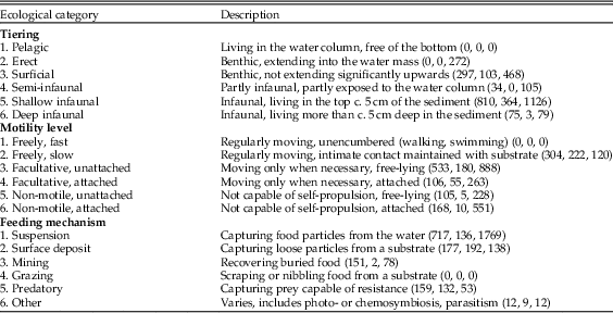
This study used a framework for ecological modes that is based on the first principles of functional morphology and developed by Bush and Bambach (Bambach et al. Reference Bambach, Bush and Erwin2007; Bush et al. Reference Bush, Bambach and Daley2007). The ecological mode of a species is defined by three axes: tiering, motility, and feeding. Each axis consists of six categorical states. The tiering axis consists of pelagic, erect, surficial, semi-infaunal, shallow infaunal, and deep infaunal. The motility axis consists of freely motile/fast, freely motile/slow, facultatively motile/unattached, facultatively motile/attached, nonmotile/unattached, and nonmotile/attached. The feeding axis consists of suspension feeding, surficial deposit feeding, mining, grazing, predatory, and other (for feeding strategies that do not fit into the previous five feeding modes). We refer readers to Bush et al. (Reference Bush, Bambach and Daley2007) for a full description of the ecospace model. Ecological-mode assignments were made at the genus level. Huber (Reference Huber2010) describes the life habits of individual bivalve families, and in the cases where genera within families are known to differ from one another, notes which genera differ and how they differ from other genera in the family. All ecological assignments were based on the life habits of the adult form. In the exceedingly rare cases where a genus occupied more than one ecological category for a given axis as an adult, the single ecological category that describes the majority of species in the genus was chosen. For the modern bivalve range data set, we were able to assign ecological modes to 1477 of 1578 species by matching species to genera.
Analyses
For the modern bivalves range data set, we first analyzed the association between ecological mode and POC flux regime. We tested for an association using an analysis of variance with post hoc comparisons estimated by Tukey’s honest significant difference method (Tukey Reference Tukey1949). We evaluated different model fits, such as inclusion of interaction effects, by comparison of Akaike information criterion (AIC) values. We conducted separate tests for Pacific and Atlantic species.
For the modern bivalves range data set, we also conducted a correlation analysis of mean POC fluxes among ecological modes comparing the mean POC values determined with the Atlantic data to those determined with the Pacific data using Spearman’s rho statistic to estimate a rank-based measure of association. This allowed us to examine whether high-energy or low-energy ecological modes were consistently found in high- or low-energy settings using independent lists of species and independent ocean basins. We also tested whether the representation of ecological modes differs between the overall higher-productivity Pacific Ocean and lower-productivity Atlantic Ocean. For the Atlantic and Pacific Oceans separately, we calculated the proportion of each species within each ecological mode. We then calculated the difference in the proportion of species within each ecological mode between the Atlantic and Pacific Oceans and compared that to the mean carbon flux of the ecological mode. We predict that ecological modes more strongly tied to higher POC fluxes will occur at higher proportions in the Pacific compared with the Atlantic due to the overall higher productivity in the Pacific. We tested this relationship using a general linear regression model with mean POC flux of the ecological mode as the independent variable and the Atlantic/Pacific ratio of the proportion of species as the dependent variable.
If different ecological modes possess different levels of range fragmentation, results obtained with the modern range data set could be biased. For the Atlantic point data set, we assessed the possibility that different ecological modes have different levels of range fragmentation. We tested this with separate ANOVAs and Tukey HSD post hoc comparisons, for feeding, motility, and tiering. Specifically, we examined whether different ecological category states within feeding, motility, and tiering can explain differences in the proportion of samples in which a species occurs. We also examined the role of data extremes on estimates of geographic-range size. If geographic ranges are artificially inflated due to extreme latitude and longitude values at the range borders, this may create errors in our estimates of POC. We tested this potential influence of extreme outliers by examining the Spearman’s rank correlation between maximum depth and latitude and the 90th and 95th percentiles and minimum depth and latitude and the 5th and 10th percentiles.
We used the fossil bivalve data set to test whether modes of life associated with higher POC fluxes in the modern oceans also first appear later in the fossil record, increase in relative diversity toward the present, or increase in relative occurrence frequency toward the present, as would be expected if Paleozoic oceans were generally associated with lower-than-modern POC fluxes. For each ecological mode, we calculated the mean, minimum, maximum, median, and standard deviation of carbon flux observed across modern genera for Atlantic and Pacific bivalves in the range data set. These values were then assigned to all fossil bivalve genera with the same ecological modes. PBDB occurrences were also assigned an ecological mode based on Knope et al. (Reference Knope, Heim, Frishkoff and Payne2015). The fossil data set allowed us to calculate the mean POC flux for the Pacific and Atlantic calibrations in two different ways. In the first, we simply took the mean POC flux of all genera extant in each time interval of the Phanerozoic. The number of PBDB occurrences is a crude approximation for the commonness of bivalve genera through time. We also calculated POC flux in each time interval by averaging across all occurrences sampled in each interval. Generalized linear models were conducted between mean POC flux as taken across ecological modes in an interval versus the interval midpoint. We also used an ordinary least-squares regression analysis to test for an association between the mean POC flux for a mode of life and its time of first appearance in the fossil record, based on the origination time of the earliest genus to exhibit that mode of life.
We constructed a simulation with the fossil bivalve data set to test whether the empirical pattern is different from simulated random trends in the mean POC flux through geologic time. We randomly shuffled (i.e., sampled without replacement) the ecological modes among the fossil genera, then assigned the Pacific and Atlantic calibrated POC fluxes to each genus and tabulated the mean POC flux through time. This procedure was repeated 1000 times, and the observed mean values were plotted against the middle 90% of simulated values in each geological time interval.
Results
Modern Bivalve Range Data Set (Atlantic and Pacific)
Mean carbon fluxes differ significantly across ecological modes in living bivalves (i.e., the unique combinations of the three niche axes) (p<<0.0001, R 2=0.25; Supplementary Fig. S1, Supplementary Tables S1–S3). A model including tiering, motility, feeding, and pairwise interactions provided the best prediction, based on AIC values, of mean carbon flux (p<<0.0001, R 2=0.26; Supplementary Table S4).
In addition to differences across ecological modes, mean carbon fluxes differ significantly across many categorical states within each of the three ecological-mode axes. First, carbon flux differs significantly across feeding modes (ANOVA: p<<0.0001, R 2=0.21). A Tukey HSD found significant differences between suspension compared with mining and predation feeding (Supplementary Table S1). Predation was significantly different from suspension and surface deposit (Supplementary Table S1). Suspension feeding and surface deposit feeding were associated with the largest carbon fluxes, whereas mining and predation were associated with the lowest flux values (Supplementary Table S1). Second, carbon flux also varied significantly across motility levels (ANOVA: p<<0.0001, R 2=0.14). Interestingly, slow-moving motile species were associated with lower carbon flux values (Tukey HSD: p<<0.0001 for all comparisons with freely motile, slow; Supplementary Table S2). Nonmotile groups were also associated with higher carbon flux values compared with facultatively motile groups (Supplementary Table S2). Finally, carbon flux varied significantly across habitat tiering levels (ANOVA: p<<0.0001, R 2=0.04); Tukey post hoc analyses show that surficial and shallow-infaunal species occur at significantly lower carbon fluxes than semi- and deep-infaunal species (Supplementary Table S3).
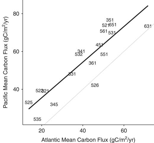
To test whether differences in mean carbon fluxes among ecological modes directly reflect energetic constraints on ecological structure versus other, unexamined factors, we tested the reproducibility of the differences between the Atlantic and Pacific Oceans. Using independent values of mean carbon flux for ecological modes by restricting the analysis to species endemic to either the Atlantic or the Pacific, we find striking consistency in the ranking of carbon flux requirements in bivalve ecological modes (Spearman’s rank correlation ρ=0.83, p<<0.0001; Figure 1). In general, suspension-feeding strategies (ecological-mode codes ending in 1) are associated with higher POC fluxes; and predation (ecological modes ending in 5) is associated with lower POC fluxes. The finding that most ecological modes are typically associated with higher flux values in the Pacific Ocean is not surprising; the Pacific is on average more productive than the Atlantic (Marra et al. Reference Marra, Weibe, Bishop and Stepien1987; Lutz et al. Reference Lutz, Caldiera, Dunbar and Behrenfeld2007).
Mean carbon flux of bivalve ecological modes in the Pacific Ocean versus the mean carbon flux of ecological modes in the Atlantic Ocean. Black line denotes the rank order correlation and the gray line represents the one-to-one value line. Numbers refer to the ecological modes, unique functional combinations, as in Table 1.

Basic ecological categories for tiering, motility level, and feeding mechanism from (Bambach et al. Reference Bambach, Bush and Erwin2007; Bush et al. Reference Bush, Bambach and Daley2007). Numbers after include the number of bivalve species in the modern range dataset, modern point dataset, and the number of bivalve genera in the fossil dataset.

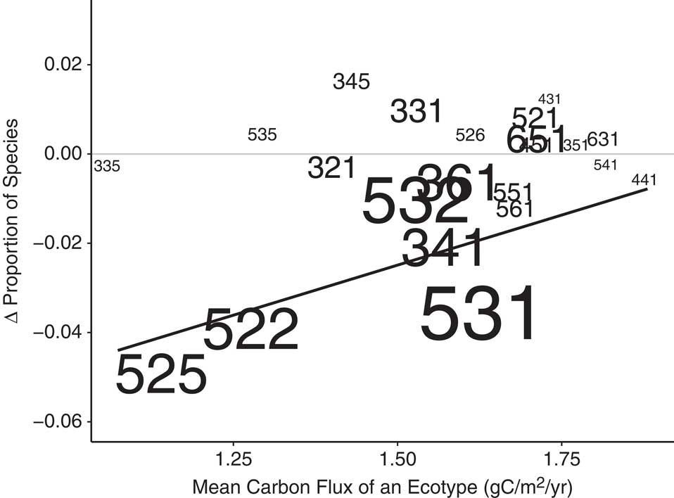
Given the difference in overall productivity levels between ocean basins, we tested another prediction: ecological modes associated with high carbon fluxes should constitute a higher proportion of the Pacific fauna and, conversely, ecological modes associated with low carbon fluxes should be more prevalent in the Atlantic due to the overall differences in productivity levels between ocean basins. This test is particularly important, because it helps to address the question of whether the causal control on the association between ecological-mode prevalence and POC flux is another factor associated with water depth, such as substrate type, and indicates that the observed correlation of ecological-mode prevalence to POC flux simply reflects the fact that many predictors correlate with water depth. The Atlantic and Pacific Oceans differ systematically in POC flux, whereas many other correlates of water depth, such as substrate type, should not differ as systematically between the two ocean basins. Consistent with POC flux playing a causal role in structuring the functional diversity of large-scale ecosystems, we find that high ecological modes associated with higher POC fluxes occur in greater proportion in the Pacific Ocean and, conversely, low carbon flux ecologies occur in greater proportion in the Atlantic (linear model: p=0.0090; Fig. 2). Thus, not only do carbon flux levels within ocean basins segregate ecological modes, but the overall taxonomic diversity within modes also varies as a function of carbon flux. Bivalve communities and regional species pools in the modern Atlantic and Pacific Oceans appear to be functionally structured by POC fluxes. This pattern could reflect differences in representation between the Atlantic and Pacific of clades within bivalves. In other words, this pattern could, in principle, be a phlyogenetic rather than an ecological pattern. We test for this possibility by testing the correlation of the number of species per family between the Atlantic and Pacific and find a strong correlation (ρ=0.721, p<<0.0001), indicating that the pattern does not reflect the rarity of certain families in the either the Atlantic or Pacific.
Change in the proportion of ecological modes between the Atlantic and Pacific Oceans versus the mean carbon flux of the ecological mode. Increases in values indicate increased representation in the Pacific and decreased representation in the Atlantic. Size of text indicates ecological-mode proportion in the data set. Numbers refer to the ecological modes, unique functional combinations, as in Table 1.

Modern Bivalve Point Data Set (Atlantic Ocean)
In our analysis of modern bivalve range data, we assume that biogeographic distributions are continuous between extremes of latitude and depth. Our findings could, therefore, be biased if different ecological modes possessed different levels of range fragmentation and, thus, that the mean POC fluxes across the continuous ranges were not representative of those experienced by the living populations. We test this assumption in our modern bivalve point data set using a Tukey HSD, post hoc comparison of the proportion of samples a species occurs in among 255 samples across the Atlantic Ocean versus different ecological modes of feeding, motility, and tiering. For motility, although the model was significant (p=0.03), the Tukey HSD test failed to find significant differences for any motility two-way comparison. For tiering, the model was not significant (p=0.11). For feeding, the model was highly significant (p<<0.0001), but the Tukey HSD only identified significant differences between groups between predatory and surface-deposit feeding and between surface-deposit feeding and suspension. However, these differences are relatively small between groups (proportion of samples for surface deposit: 1.9%; predation: 4.5%; and suspension: 2.2%, Supplementary Fig. S2).
Biogeographic ranges in our modern bivalve range data set are defined by maximum geographic extents. If extreme values were far from and uncorrelated with the highly occupied region of each species’ range, our use of extremes could yield mean POC flux values far from the true values experienced by the living populations. To test the assumption that the extreme values used are correlated with the edges of the more densely occupied ranges and not influenced by a few severe outliers, we examine the correlations between maximum geographic extent and range quantiles in our modern point data set (Supplementary Fig. S3). The correlations are extremely high for maximum latitude and the 95th (ρ=0.997, p<<0.0001) and 90th percentiles (ρ=0.991, p<<0.0001). For minimum latitude, the correlations with the 10th (ρ=0.941, p<<0.0001) and 5th (ρ=0.976, p<<0.0001) percentiles are also high. A similar pattern occurs in the correlations for maximum depth versus 95th (ρ=0.985, p<<0.0001) and 90th (ρ=0.967, p<<0.0001) percentiles, as well as minimum depth and the 10th (ρ=0.935, p<<0.0001) and 5th percentiles (ρ=0.971, p<<0.0001). This finding demonstrates that the effect of outliers is minimal in our point data set and likely to be small as well in the larger range data set that we used to assess the relationship between POC flux and the diversities of different ecological modes. Moreover, we find strong correlation for this deep-sea data set where sampling is comparably poorer than for shallow seas, from which most of the larger data set derives. Given the overwhelming proportion of shallow-water species in our modern bivalve range data set analysis (<500 m maximum depth, the median of the maximum depth values in our data set is 196 m, 62% of species have maximum depths shallower than 500 m), this suggests the effect of data extremes will add minimal bias to our analyses.
Fossil Bivalve Data Set
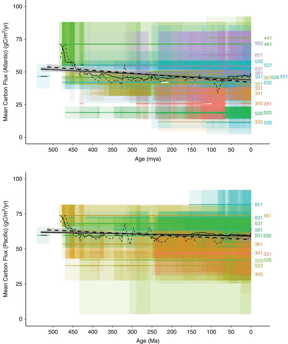
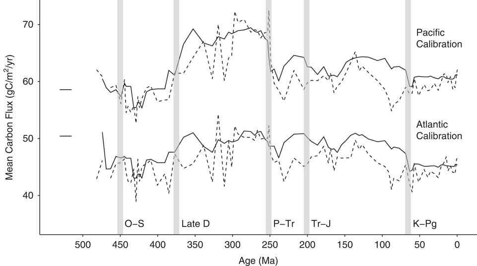
We test the hypothesis that an increase in energy availability through time stimulated the taxonomic and functional diversification of bivalves (Vermeij Reference Vermeij1977, Reference Vermeij1995; Bambach Reference Bambach1993) by applying modern organic carbon fluxes for each ecological mode to the ecological modes of fossil bivalve genera (Supplementary Table S5). In so doing, we find evidence of a decreasing temporal trend in the mean POC flux across genera, regardless of whether we assigned the POC flux value to a mode of life based on the values obtained from the living Pacific (p<<0.0001) or Atlantic species (p<<0.0001; Figs. 3, 4). We also conducted the analysis after calculating a weighted mean POC flux based on the number of bivalve occurrences in the PBDB for each mode of life in each geological interval. This alternative approach of weighting by fossil occurrence frequency rather than genus diversity also indicates a decrease of mean POC flux per occurrence through time, regardless of whether the analysis is calibrated to the modern Atlantic or Pacific values (p<<0.0001).
Carbon fluxes implied by the relative diversities of bivalve ecological modes across Phanerozoic time. Each mode is plotted using Atlantic (top) and Pacific (bottom) calibrations. Also plotted for each mode is the 95% confidence interval for the ecological-mode calibration. Both the lines and the confidence intervals are plotted as transparent so that intervals of higher diversity appear as more darkly shaded regions. Colors (see online version) correspond to modes. Black, solid, straight line is the regression line between the geologic time and the mean of carbon flux value of all genera in that interval. Black, solid, varied line is the LOESS fit of the mean carbon flux values across time. Dashed lines are the same as above, except they are based on means of PBDB occurrences rather than genera. The top panel reflects carbon flux values based on modern Atlantic Ocean values, and the bottom panel reflects carbon flux values based on modern Pacific Ocean values. Numbers refer to the ecological modes, unique functional combinations, as in Table 1.

Changes in mean carbon flux across bivalve ecological modes for bivalve genera through time. Solid line is the mean carbon flux across ecological modes. Dashed line is the mean of PBDB occurrences rather than genera.

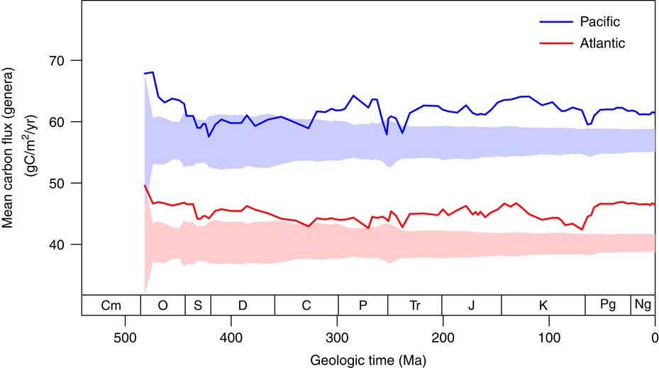
As a further test for an influence of POC flux on the presence of modes of life, we compared the timing of first occurrence of modes of life with their associated POC flux values using both the Atlantic and Pacific calibrations. In each case, we find no significant correlation between POC flux and age of first occurrence (Atlantic: p=0.44; Pacific: p=0.09). Our randomization test shows that both the Pacific and Atlantic calibrations produce POC fluxes through time that are higher than expected if ecological modes were randomly distributed among genera (Fig. 5). This test shows that although there is no directionality in the mean POC flux through time, ecological modes are not randomly distributed among genera. Specifically, genera with high POC flux calibrations tend to have longer stratigraphic durations. Because genera with higher fluxes are longer lived, they occur in more time intervals and thus weight each time interval toward higher values. In summary, we find no statistical evidence that modes of life associated with higher POC fluxes in the modern oceans have either appeared later in the fossil record or increased differentially in genus diversity or fossil occurrence frequency across geological time. Each of these findings is inconsistent with the hypothesis that bivalve diversification has been driven by a systematic increase in mean POC flux of global oceans across hundreds of millions of years.
Observed mean carbon fluxes across geologic time compared with null expectations of a random association between fluxes and fossil bivalve genera. The solid lines represent the observed mean trends for the Pacific (top) and Atlantic (bottom) calibrations. The shaded intervals mark the middle 90% of values based on 1000 randomizations. In each randomization, each fossil genus was randomly assigned a carbon flux from the total pool of flux calibrations, and the mean flux was calculated for each time interval from the Ordovician through the Pleistocene.

Discussion
Our data demonstrate that ecological niche axes in modern bivalves, as measured here, are correlated with the available environmental energy. More specifically, in modern bivalves, the basic functional traits of feeding mode, tiering level, and motility level are associated with their relative prevalence in low- or high-food settings (Test 1). The strong consistency between the rank orders of ecological modes based on carbon flux between the Atlantic and Pacific Oceans, observed across independent lists of endemic species, implies that the association between ecological mode and carbon flux is not an artifact of indirect connections but, rather, a fundamental aspect of these ecological modes (Test 2). Moreover, the higher resolution, point-sample data set of modern bivalves demonstrates that these findings are robust to potential biases associated with using range limits and assuming continuous occupancy (Test 4).
Clear and reproducible differences occur in the typical carbon flux levels occupied by different ecological modes. In some cases, these findings contrast with expectations. For example, greater motility in bivalves is associated with lower POC regions of the oceans. This finding contrasts with the observation that greater movement velocity is associated with increases in metabolic demand in vertebrates (Taylor et al. Reference Taylor, Schmidt-Nielsen and Raab1970; Alexander Reference Alexander2005). Mollusk species with greater burrowing speeds also incur greater metabolic costs (Trueman Reference Trueman1983). The association of greater motility with lower POC fluxes in bivalves may reflect the lower velocities and more infrequent movements of motile bivalves relative to their vertebrate counterparts, leading to motility constituting a smaller portion of the overall energy budget in motile bivalves. As expected, deeper infaunal species are also associated with higher POC regions, mirroring prior work detailing that the sediment depth of particle mixing by animal activity increases with increasing POC flux (Smith and Rabouille Reference Smith and Rabouille2002).
Also, contrary to expectations, suspension feeding was associated with high POC regions. Predation is typically seen as a high-energy strategy. Indeed, in vertebrates (Carbone et al. Reference Carbone, Teacher and Rowcliff2007) and mollusks (Vladimirova Reference Vladimirova2001; Vladimirova et al. Reference Vladimirova, Kleimenov and Radzinskaya2003) alike, mass- and temperature-adjusted metabolic rates are higher in carnivorous groups. Moreover, higher trophic levels are predicted at higher environmental productivities, as more prey biomass is required to offset energy loss between trophic levels (Post Reference Post2002b). Thus, the documented increase in predation through time (Vermeij Reference Vermeij1977, Reference Vermeij1995; Bambach Reference Bambach1993) has been hypothesized to reflect increases in food availability across geological time (Bambach Reference Bambach1993). For example, Bambach (Reference Bambach1993: p. 381) states, “Predation is an energetic mode of life and the survival of predators depends on abundant energy acquisition ... It is apparent that the modern fauna, to support both higher biomass and more energetic modes of life, requires more food and energy than did the Paleozoic fauna.” Yet, our findings demonstrate that predatory feeding strategies in bivalves are not preferentially associated with more productive regions of the ocean. Predation in bivalves occurs among the “Septibranch” families within the subclass Anomalodesmata (Beesley et al. Reference Beesley, Ross and Wells1998). The siphon is either rapidly extended into the water column to capture small swimming prey (e.g., in Cuspidaria cuspidata) or quickly extended across the sediment to capture crawling prey (e.g., in Poromya illevis) (Beesley et al. Reference Beesley, Ross and Wells1998). Feeding bouts in predators occur on concentrated food resources in the form of discrete animal prey. Our finding that predatory bivalves occur typically in environments characterized by low carbon fluxes suggests that predation, although requiring more energy per unit mass, does not require higher overall ocean productivity. Rather, food must be concentrated into discrete prey items and consumption must be efficient through targeted behaviors. In addition, as overall POC flux decreases, the temporal and spatial patchiness of POC availability will increase (McClain and Schlacher Reference McClain and Schlacher2015), favoring ecologies like predation adapted for ephemeral food resources. In contrast, suspension feeders require a continuous supply of suspended particulate matter at a density high enough to offset the energetic costs of filter feeding; thus, the link to regional carbon fluxes is more direct (McClain and Lundsten Reference McClain and Lundsten2015). This contrast may also be enhanced by the fact that bivalve predators rely primarily on ambush strategies rather than pursuit.
Ecological differences among ocean basins, correlated with differences in POC, provide evidence that overall food availability at broad scales can shape the ecology of the regional to global biota (Test 3). The differences in total carbon flux between the Atlantic Ocean and Pacific Ocean determined the relative proportion of specific bivalve ecologies. Low carbon flux ecologies, although occupying regions of higher carbon fluxes in the more productive Pacific Ocean, were not as well represented in the Pacific. High carbon flux ecologies, while occurring in lower carbon fluxes in the less productive Atlantic Ocean, were not as well represented in the Atlantic. Thus, overall ocean food availability determined the relative dominance of different ecological strategies, consistent with hypotheses that energy availability at a global scale may significantly influence the overall diversity and ecological structure of the marine animal biosphere. These findings also provide a direct link between the energy demand of different ecological strategies and broad-scale patterns in beta diversity spanning energy gradients (Melo et al. Reference Melo, Rangel and Diniz-Filho2009; Andrew et al. Reference Andrew, Wulder, Coops and Baillargeon2012; McClain et al. Reference McClain, Stegen and Hurlbert2012b; Veech and Crist Reference Veech and Crist2007; McClain and Rex Reference McClain and Rex2015). In addition, the offset of the Pacific Ocean toward both higher productivity levels and greater prevalence of species characterized by high-POC modes of life provides an additional indication that the association between modes and POC flux does not simply reflect the fact that some other potential controls on ecological structure correlate with water depth. If, for instance, the association of POC flux with mode of life prevalence were in fact produced by the correlation of both POC flux and some other control on ecosystem structure (e.g., substrate type, water energy level), then the offset would not be expected. However, many environmental variables do not vary systematically with depth to the degree and strength of POC (Supplementary Fig. S4). Oxygen and temperature only vary significantly within the shallowest 1000 m but not substantially after (Supplementary Fig. S4). Salinity does not vary significantly with depth in the regions studied here. Moreover, it has been shown previously that the most important driver of bivalve species, trait, and phylogenetic community structure in the Atlantic Ocean is POC (McClain et al. Reference McClain, Stegen and Hurlbert2012b). Factors other than POC flux may correlate with depth, but the available evidence points toward a direct effect of POC on ecosystem structure as an important and measurable one. Expanded data sets will be required to test for and deconvolve the further influences of additional factors, such as substrate type, water energy, and water temperature.
We test some of the assumptions of our coarse range data set with a higher-resolution, point-sample data set. We find that assuming continuous ranges within a species biogeographic range extent and assuming that the biogeographic range is defined by the maximum reported bathymetric and latitudinal extent are unlikely to introduce substantial bias into our analyses (Test 4). However, several additional caveats should be noted that may impact our analysis and interpretations. One caveat of our analysis is that we deal with species presence/absence and not abundance of the species through its biogeographic range. The finding that predatory species typically inhabit lower, not higher, POC flux does not preclude that predator species could be more abundant in higher POC areas. We lack oceanic-scale data sets for the modern oceans that also contain abundance data, such as the breeding bird surveys for terrestrial systems, that would allow testing of this possibility. Our modern point data set unfortunately does not allow testing of this scenario, given the low number of predatory species. Our analysis is restricted to bivalves and assumes, similar to many previous studies on mammals and birds (Mönkkönen et al. Reference Mönkkönen, Forsman and Bokma2006; Hawkins et al. Reference Hawkins, Diniz-Filho, Jaramillo and Soeller2007; Okie and Brown Reference Okie and Brown2009; Buckley et al. Reference Buckley, Davies, Ackerly, Kraft, Harrison, Anakcer, Cornell, Damschen, Grytnes, Hawkins, McCain, Stephens and Wiens2010), that one clade can be treated as a competing assemblage. However, bivalves interact with species in several other groups (e.g., gastropods, arthropods, and polychaetes) as predators, prey, and competitors. Thus, the overall prevalences of ecological modes in ecosystems and their variations across POC flux levels may differ for the whole biological community relative to what we observe in bivalves. The data required to test this possibility are not yet available.
Application of the modern calibrations to the diversity and occurrence histories of marine bivalves does not obviously conform to the prediction of the energy-limitation hypothesis, in which low POC fluxes early in the Paleozoic would have favored ecological modes associated with low POC fluxes in the modern ocean, and higher POC fluxes by Cenozoic time would have favored ecological modes associated with higher POC fluxes in the modern oceans (Test 5). Instead, we find that Paleozoic oceans were not dominated by ecological modes associated with low POC fluxes, and the modern oceans are not substantially more skewed toward modes associated with high POC fluxes in the modern. In fact, the mean value across all genera and all occurrences has decreased slightly across Phanerozoic time (Figs. 3, 4). In addition, the first appearance times of modes of life do not exhibit any trend toward the later appearance of modes associated with higher POC fluxes in the modern oceans.
Four scenarios, not mutually exclusive, may reconcile the paleontological evidence for increase in per capita metabolic rates (Bambach Reference Bambach1993; Finnegan et al. Reference Finnegan, McClain, Kosnik and Payne2011; Payne et al. Reference Payne, Heim, Knope and McClain2014) with the finding presented above that Paleozoic oceans were not preferentially occupied by bivalves with ecological modes typical of low flux environments. First, the relationship between carbon flux and specific ecological modes may have changed across time. For example, suspension feeding may be shifted toward higher POC environments in the modern oceans than it was in the past, which would reconcile arguments for low Paleozoic food supply (e.g., Bambach Reference Bambach1993, Reference Bambach1999; Vermeij Reference Vermeij1995) with the abundance of suspension feeders on the Paleozoic seafloor. Such a change could have occurred, for example, because the identities of the dominant phytoplankton in the ocean have changed across time (Falkowski et al. Reference Falkowski, Katz, Knoll, Quigg, Raven, Schofield and Taylor2004). The vast changes in the ecological structure of marine ecosystems that have occurred across geological time (reviewed in Bush and Bambach Reference Bush and Bambach2011) add to the challenge of calibrating productivity–ecology relationships in deep time. On the other hand, the correspondence between the Atlantic and Pacific Oceans (Fig. 3) using nonoverlapping sets of species for calibration points toward some stability in this relationship. Second, the calibration may be appropriate to environments inhabited by bivalves, but bivalves were only able to occupy a small fraction of Paleozoic oceans with POC fluxes close to modern values, while large areas remained too starved of food to support bivalves at all. The greater prevalence of unfossiliferous rocks deposited in open-marine settings during Paleozoic time relative to the post-Paleozoic (Peters Reference Peters2007) lends credence to this scenario, as does the gradual expansion of bivalves from nearshore environments to open-shelf and deeper-water habitats and the associated retreat of brachiopods to deeper-water habitats across Phanerozoic time (Sepkoski and Miller Reference Sepkoski and Miller1985; Tomasovych Reference Tomašových2006). On the other hand, bottom-water anoxia may have been as important as low food availability in excluding animals from these environments (Peters Reference Peters2007; Meyers et al. Reference Meyers, Ridgewell and Payne2016). Third, Paleozoic oceans may have had POC fluxes similar to, or even higher than, modern values, but bivalves may have been less effective at capturing that organic matter prior to it being respired by microbes or other animals. High prevalence of hypoxic and anoxic environments during Paleozoic time may have excluded bivalves and other animals from many benthic marine environments, leaving more organic matter available to microbial respiration than during post-Paleozoic time. However, these hypoxic and anoxic environments could, alternatively, reflect lower atmospheric oxygen concentrations relative to the present rather than from higher levels of primary production. Fourth, the calibration may be appropriate to the whole ocean but has more limited predictive capability when analyzing a fossil record that is mostly biased toward the preservation of shelf environments and that has shifted, in the best-sampled regions of North American and western Europe, from a predominance of preserved tropical paleolatitudes dominated by carbonate sediments to a predominance of preserved extratropical paleolatitudes dominated by siliciclastic sediments. In principle, temporal trends in the bias against preservation of small-bodied or aragonite-shelled bivalves could generate or remove trends in the apparent records of modes of life. In practice, there is no strong evidence for mineralogical bias introducing trends into the fossil record of marine mollusks (Kidwell Reference Kidwell2005). The bias against the preservation and recovery of small-bodied fossil mollusks may have decreased over time, but it is pronounced even in the Cenozoic (Cooper et al. Reference Cooper, Maxwell, Crampton, Beu, Jones and Marshall2006). Regardless of the precise causes, however, energetic calibration from bivalves does not provide positive support for food availability strongly controlling the pattern of ecological exploration across evolutionary time within this class of animals.
Overall, our findings support the contention of Harmon and Harrison (Reference Harmon and Harrison2015) that ecological processes, in this case energetic limits from the supply of fixed carbon, only weakly and inconsistently limit global diversity and ecological structure across evolutionary timescales. In part, this lack of pattern may result from heterogeneity across scales in carbon flux regimes (Lutz et al. Reference Lutz, Caldiera, Dunbar and Behrenfeld2007). Despite global changes in overall productivity, lower- and higher-productivity regions will coexist across spatial gradients, offering opportunity to both low– and high–energy demand species. Beta diversity varies over energy gradients, and species appear to have specific and often narrow energetic niches (McClain et al. Reference McClain, Stegen and Hurlbert2012b). Furthermore, our results demonstrate that these large-scale spatial patterns in heterogeneity of energy availability lead to differences in the proportions of specific ecological modes. Whereas resource limits may impact ecological diversity and structure at local to regional scales (Hurlbert and Stegen Reference Hurlbert and Stegen2014; Rabosky and Hurlbert Reference Rabosky and Hurlbert2015), at global scales these effects are averaged out (Harmon and Harrison Reference Harmon and Harrison2015).
Conclusions
Quantification of the relationship between POC flux and ecological modes in bivalves demonstrates an important control of energy availability on ecological structure in modern marine communities. There are statistically significant differences in the typical POC flux experienced by species with different ecological modes and, moreover, these differences are reproduced in the Atlantic and Pacific Oceans across entirely distinct sets of species. In addition, the overall higher primary productivity and carbon flux in the Pacific Ocean is associated with a greater relative diversity of species characterized by high carbon flux–associated ecologies. Thus, energy availability appears to directly influence the ecological structure of modern marine bivalve communities by altering the competitive balance among ecological strategies. Applying these findings to the fossil record yields unexpected results. Because suspension-feeding strategies are often associated with high POC fluxes, whereas predation within bivalves is more prevalent at low to intermediate POC fluxes, the Phanerozoic trend toward greater levels of predation and proportionally fewer suspension-feeding taxa does not imply a global-scale shift toward higher levels of POC flux in the oceans, contrary to many previous suggestions (Vermeij Reference Vermeij1977, Reference Vermeij1995; Bambach Reference Bambach1993; Martin Reference Martin2003). Instead, the ecological history of bivalves is more consistent with relatively stable levels of fixed carbon availability in the oceans across time. These findings imply that the Phanerozoic diversification of marine animals and the differential diversification of predators likely reflect factors other than expansion at the base of the food chain. Instead, it appears more probable that animals have progressively benefited from changes in the taxonomic identities and nutrient value of the dominant primary producers and have become more efficient at capturing a greater fraction of primary productivity before it can be respired by microbes or other animals.
Acknowledgments
Funding was provided by National Science Foundation grant EAR-1151022 (to J.L.P.) and the Stanford School of Earth, Energy, and Environmental Sciences.
Supplementary material
Data available from the Dryad Digital Repository: https://doi.org/10.5061/dryad.v5978