1 Introduction
Automated planning (AP) is the branch of Artificial Intelligence pivoted on the formulation of a plan: a series of actions guiding the transition of the system from the initial state to the goal, accomplishing a required task in the process. Each action requires a certain number of preconditions to be fulfilled in order to be applied to a particular world state. Upon application, each action changes the world state with its induced effects. These actions can be represented by actions models: the blueprints of the domain-specific actions. AP came into light in the 1960s when research in the fields of operations research, theorem proving and studies into human problem solving started gathering steam, with the intent of solving problems that were being posed by the field of robotics among many others. The STRIPS (STanford Research Institute Problem Solver) system (Fikes & Nilsson, Reference Fikes and Nilsson1971) was used to control and plan the movement of an autonomous robot called Shakey (Nilsson, Reference Nilsson1984) as it pushed a series of boxes through a series of interconnected rooms. This is the perfect illustration of the application of AP to execute a task in a real life scenario. Planning, however, cannot be conducted in the absence of domain knowledge, which describes the actions that can be executed, serving as the information base to plan upon. This is where Knowledge Engineering (KE) finds its place in the domain of planning.
KE for AP is the process that deals with the acquisition, formulation, validation and maintenance of planning knowledge, where the essential output is the domain model (Jilani et al., Reference Jilani, Crampton, Kitchin and Vallati2014). The main issue of current KE approaches for encoding domain models is that they require specific expertise which can only be furnished by a domain expert. This expert, in theory can, due to his limited knowledge of the real-world domain, introduce some human-induced error in the encoding. In these situations, the success of the AP systems fully depends on the skills of the expert who defines the action model. This among others is the reason why AP, having enjoyed many feats and resounding successes in the aforementioned fields, it continues to suffer from its share of drawbacks.
Principal out of these drawbacks is the effort surrounding the creation of action models for complex domains. While it is possible to codify action models for simple domains, it remains laborious to do so for some complex real-world domains. Real-world planning domain models are hard to develop, debug and maintain. As planners and applications become larger, the challenge of engineering planning domain models becomes more magnified (McCluskey et al., Reference McCluskey, Richardson and Simpson2002). Moreover, given the sheer difficulty in generating planning domain models, many users are not exploiting AP but easier though less-efficient approaches. It is worth pointing out that KE tools for encoding domain models are, usually, not very well known outside the planning community (Shah et al., Reference Shah, Chrpa, Jimoh, Kitchin, McCluskey, Parkinson and Vallati2013).
With the intent of assisting domain experts, the planning community is developing systems to automatically acquire AP models (Jiménez et al., Reference Jiménez, De La Rosa, Fernández, Fernández and Borrajo2012). Machine learning (ML) seems to be a useful tool for these systems to automate the extraction, refinement, organization and exploitation of knowledge from plan traces or user preferences. ML is viewed as a potentially powerful means of making an agent (independent entity which perceives the world and performs actions accordingly) autonomous, while compensating for the expert’s incomplete domain knowledge. The work done in ML goes hand in hand with the long history of domain independent planning, as the techniques developed as a part of this effort could be applied across a myriad of domains to accelerate planning. In most cases, the learning techniques introduced into planners were extensively customized to the specific architecture of the application domain. Therefore, any new and more powerful learning technique required programming effort to replace an existing one. These factors might explain why the planning community appears to have paid less attention to learning till the late 1990s. However in recent times, with the explosion in computing power and the influx of ML techniques into a myriad of computing fields, ML seems to have staged its comeback since the early 2000s.
This article is pivoted on ML techniques which allow the learning of the underlying planning model from a given set of traces consisting of plan executions. The employed learning techniques vary widely in terms of context of application, technique of application, adopted learning methodology and knowledge learned. The article begins with an introduction to the domain of AP to the reader (Section 2), followed by an a description of certain key criteria that help in the characterization of the various learning systems (Section 3). It then mentions interesting learning approaches in the literature (Section 4), proceeds to highlighting some persisting open issues (Section 5) with the discussed approaches, concluding with a roundup of the paper (Section 6).
2 Formulation and representation
AP is a means-end reasoning, that is, participating agents decide how to achieve a goal given a set of available and applicable actions. These agents interact with the environment by executing actions which change the state of the environment, gradually propelling it from its initial state toward the agents’ desired goal. This transition can also be regarded as a solution to a planning problem the agent in question is looking to resolve. We begin with some definitions of fundamental concepts.
Definition 1 (Planning Problem). A planning problem is a triplet P=(STS; s 0 ; g) composed of:
∙ the initial state s 0 of the world,
∙ the goal g, (set of propositions representing the goals to achieve), belonging to the set of goal states S g , and
∙ the state transition system STS responsible for changing the world state by action application.
Definition 2 (STS). The STS in the previous definition is formally a 3-tuple (S; A; α) further composed of
∙ S={s 1, s 2, … s n } as the set of states,
∙ A=[a 1, a 2, … a n ] as the set of actions. Here each action aεA is defined in the form of the aggregation of three lists, namely (pre; add and del). These are the pre list (predicates whose satisfiability determines the applicability of the action), add list (predicates added to the current system state by the action application) and the del list (predicates deleted from the current system state upon action application), respectively. The listing of all the applicable actions in a domain is called the action model.
∙ δ: (S×A*→S) is the state transition function (Ghallab et al., Reference Ghallab, Nau and Traverso2004).
All the aforementioned elements in this section contribute to the formulation of a plan.
Definition 3 (Plan). A plan, given an initial state of the system, goal, and an action model, is a sequence of actions π=[a 1 , a 2 , … a n ] that drives the system from the initial state to the goal.
The transition from the initial state to the goal is driven by the previously mentioned transition function in Definition 1 (Ghallab et al., Reference Ghallab, Nau and Traverso2004):
 $$\delta (s,\pi ){\equals}\left\{ {\matrix{ s & {{\rm if}\left| \pi \right|{\equals}0} \cr {\delta (\delta (s,a_{1} ),[a_{2} ,\,\ldots\,a_{k} ])} & {{\rm if}\,precond(a_{1} )\,\,\subseteq\,s} \cr } } \right.$$
This transition function, when applied to the set of the current state and the applicable action, produces the next state as:
 $$s_{{i{\plus}1}} {\equals}\delta (s_{i} ,a){\equals}(s_{i} {\minus}del(a)){\cup}add(a)$$
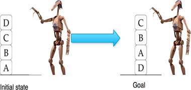
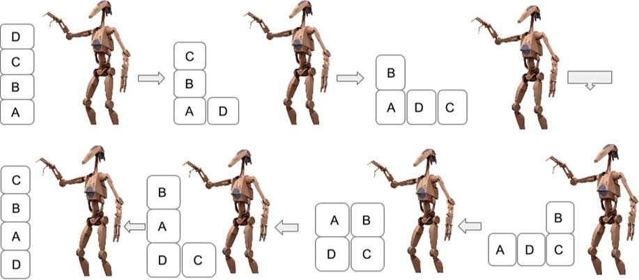
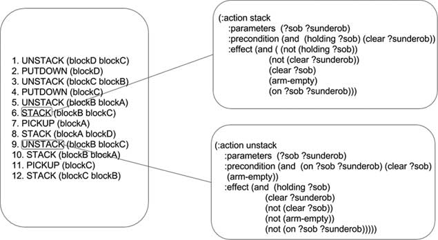
This transition function, when successively applied to the resulting intermediate states at each step, leads to the goal. Each such action sequence, complete with initial state and goal information (and occasionally intermediate state information), constitutes a trace. These traces can either be in the form of action sequences (as represented in Figure 4) or action sequences interleaved with intermediate states. We explain the notion of traces in the form of a concrete example. AP defines a certain number of world domains, one of the most famous ones being Blocksworld (Winograd, Reference Winograd1972). It consists of a set of blocks resting on a table, the goal being to build one or more piles of blocks. However, only one block may be moved at a time: either placed on top of another block or on the table. An example of action sequences in this domain is seen in the Figure 4. A snapshot of a state-action interleaved trace for the first two actions in Figure 4 is given as:
UNSTACK (blockD, blockC), (holding (blockD), not (armempty), clear (blockC)), PUTDOWN (blockD)
While good in theory, the creation of models in the case of complex domains is a non trivial task. While it is possible to codify, debug and maintain action models pertaining to simple toy domains, it remains laborious, unfeasible and sometimes impractical to do so for some complex real-world domains. The amount of effort needed to encode and maintain accurate action blueprints is significant. There is also no ‘one size fits all’ strategy. Thus, we seek help from various ML techniques which allow learning of the underlying action model from traces produced as a result of plan execution. This model can ideally be re-injected into the planner for further planning purposes. The ML techniques to learn from these traces broadly fall into one of the following categories:
∙ Online: learning occurs during the execution phase (Zimmermann & Kambhampati, Reference Zimmerman and Kambhampati2003). The system can start learning as soon as the generation phase is complete. This kind of learning never stops, thus allowing the continuous correction and improvement of an incorrect model and adaptation to changing environment characteristics. On the flip side, the cost of learning is added to the cost of planning, augmenting the time window in which execution occurs.
∙ Offline: one-shot learning exercise from traces. It allows a decoupling of the learning and planning phases, ensuring that the cost of learning is not added to that of planning. However, this one-time learning also means that in case of the injection of an ill-defined domain, the planner may never be able to recover before the end of the planning and the beginning of the learning phase, thus staying blocked. Offline learning is the more popular learning mechanism.
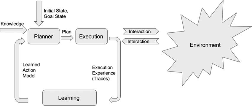
Given the aforementioned information, our learning problem can be formulated as follows: given a set of plan traces T, to learn a domain model
 $$m$$
encompassing all the domain-applicable actions which best explains the observed plan traces (see Figure 1).
Formulation and representation

We explain the aforementioned definitions in the form of a concrete example. A sample problem in the Blocksworld domain with its solution sequence is represented in the Figures 2 and 3.
Problem definition

Solution steps

AP problems and domains are typically represented in a standard language called the Planning Domain Definition Language (PDDL). It has been the official language for the representation of the problems and solutions in all of the International Planning Competitions which have been held from the year 1998 onwards.
The PDDL representation of the actions and the sequence of steps leading to the final block configuration can be summarized in the Figure 4. The left of the figure represents the sequence of actions of the Blocksworld domain, namely:
 $$pickup,putdown,stack,unstack$$
. The right of the figure represents a magnified view into two of the four actions, namely
 $$stack$$
and
 $$unstack$$
. In the PDDL representation of these actions, the name of the action follows the
 $$\,\colon\,action$$
tag. Similarly, the parameters constituting the action signature follow the
 $$\,\colon\,parameters$$
tag. The preconditions and effects of the action are represented as a conjunction of predicates follow the :precondition (equivalent to the pre list in Definition 2) and :effect (equivalent to the add and del lists in Definition 2) tags, respectively.
Planning Domain Definition Language representation of the actions stack and unstack in the Blocksworld domain

Choosing a good representation language which accurately models every action effect the system might encounter and no others is essential. Any extra modeling capacity is wasted and complicates learning, since the system will have to consider a larger number of potential models, and be more likely to overfit (Pasula et al., Reference Pasula, Zettlemoyer and Kaelbling2007).
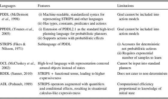
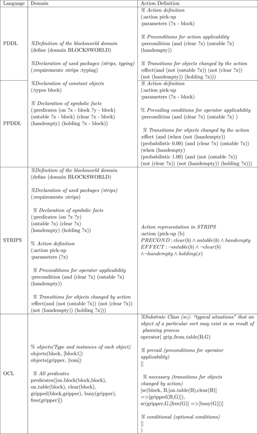
Some languages in the domain of AP and their features are summarized in the Table 1. We return to our example of the Blocksworld domain, and refer to the action ‘pick-up’ which represents the picking up of a block from the table or from another block. A syntactic representation of the action ‘pick-up’ of the Blocksworld domain in four prominent languages (described in Table 1) can be found in Table 2.
Representation languages in Automated Planning

PDDL=Planning Domain Definition Language; PPDDL=Probabilistic PDDL; STRIPS=STanford Research Institute Problem Solver; OCL=Object-Centered Language; RDDL=Relational Dynamic Influence Diagram Language; ADL=Action Description Language.
Representation of action ‘pick-up’ of the Blocksworld domain in various languages

PDDL=Planning Domain Definition Language; PPDDL=Probabilistic PDDL; STRIPS=STanford Research Institute Problem Solver; OCL=Object-Centered Language.
3 Characteristics of learning systems
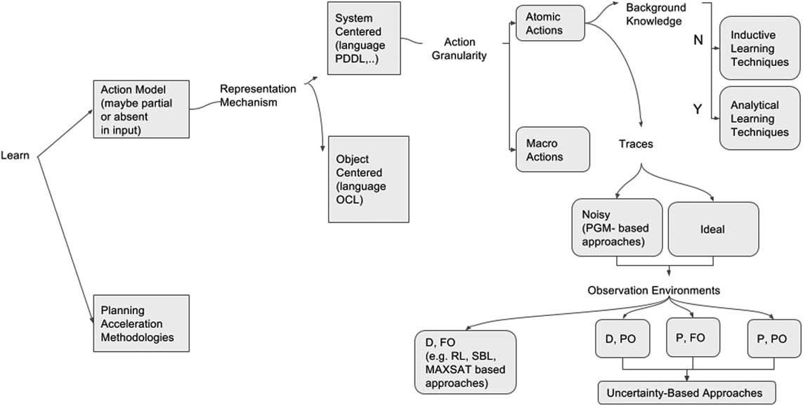
During the course of this bibliographical review, we have been able to identify certain key criteria which help us characterize the works in this paper. These criteria are described in the following subsections. These criteria also serve as a guideline for creating a ‘cheat sheet’ with the intent of helping researchers starting out in the domain to choose a specific learning technique based on the characteristics defined in this section. This ‘cheat sheet’ (see Figure 5) is not exhaustive, and conceptualized bearing in mind the methodology adopted by the paper and the learning techniques discussed in Section 4. The branch in this figure dedicated to the learning of heuristics is not detailed as it is beyond the scope of this paper. The characteristics are detailed in the subsections below.
Guideline for choosing appropriate learning approach based on input requirements. PDDL=Planning Domain Definition Language; OCL=Object-Centered Language; D=Deterministic; P=Probabilistic; FO=Fully Observable; PO=Partially Observable; MAX-SAT=Maximum Satisfiability; PGM=Probabilistic Graphical Model; RL=Reinforcement Learning; SBL=Surprise Based Learning

3.1 Representation mechanism
This section tries to classify approaches based on the viewpoint the learning system is observed from. The learning system can be seen as:
∙ Object-centered representation: each object in the domain manipulated by an action is represented by a single-parameterized state machine. The action model is generally represented in OCL (Object-Centered Language).
∙ System-centered representation: a plan is viewed as an interleaved sequence of states and actions representing the transition of the system from the initial state to the goal. The action model in this case is generally represented in the form of PDDL and its sub-languages or variants.
3.2 Inputs to the system
The inputs to the learning system as well as some other characteristics (quality, quantity, etc.) go a long way in determining the output and its quality. The inputs to the system may include: the model, the background knowledge (BK) and the traces; all three in varying capacities.
3.2.1 Model
Before the learning phase begins, the action model may exist in one of the following capacities:
∙ No model: this refers to the fact that no information on the actions that constitute the model is available in the beginning, and the entire model must be learnt from scratch.
∙ Partial model: some elements of the model are available to the learner in the beginning, and the model is enriched with more knowledge at the end of the learning phase.
3.2.2 Background knowledge
BK is mostly required only in the absence of complete and correct domain knowledge. The availability of this BK is inversely proportional to the planning effort required. For example, in the Blocksworld domain, ‘only one block can be on top of some other block’ or ‘a block being held means that the robotic arm is not empty’ is an illustration of BK. To compensate for the absence of domain knowledge, this BK may also comprise of object type definitions as well as predicate and intermediate state information (Jilani et al., Reference Jilani, Crampton, Kitchin and Vallati2014).
In most cases, it restricts the possible action choices at every system state, thus speeding up planning. This BK, however, may also be difficult to acquire. Depending on the presence or absence of BK, the associated learning techniques may either be classified as analytical or inductive, respectively. These techniques are discussed in detail in Section 4.1.
3.2.3 Traces
Traces are the residue or the proof of the execution of a series of actions in a domain. They represent a summary of the executed action and the resulting state of the world. These plan execution traces may be classified into pure or adulterated as follows:
∙ Noisy: the traces can be adulterated because of sensor miscalibration or faulty annotation by a domain expert. For example, AMAN (action-model acquisition from noisy plan traces) (Zhuo et al., Reference Zhuo, Nguyen and Kambhampati2013) falls into this category.
∙ Ideal: there is no discrepancy between the ideal action and the recorded action. For example, OBSERVER (Wang, Reference Wang1996).
3.3 System outputs
3.3.1 Action granularity
Irrespective of whether the trace is represented in form of action sequences or state–action interleavings, the actions can be classified as atomic or grouped. Atomic actions are unitary actions applied to a system state to effectuate a transition. Macro-actions, on the other hand, are a group of actions applied at a time point like a single action, representing high-level tasks while encompassing low-level details (Newton et al., Reference Newton, Levine, Fox and Long2007, Reference Newton, Levine, Fox and Long2008, Reference Newton and Levine2010). From a broader perspective, macros are like procedures in the programming realm. They are promising because they are capable of aggregating several steps in the state space, and providing extended search space visibility to the planner. Some merits of using macros include:
∙ Macros generated from plans of smaller problems are scalable and can be evaluated against larger problems.
∙ Macros allow planning of several steps at a time and allow for re-usability in plan snippets. Knowledge acquired from macros can be integrated into the planner or encoded into the domain (Newton et al., Reference Newton, Levine, Fox and Long2007, Reference Newton, Levine, Fox and Long2008, Reference Newton and Levine2010).
Some limitations are as follows:
∙ They increase the processing time of the planner, adding more branches in the search tree at every point in time. However, the problem is significantly reduced by search tree pruning used by many recent planners (Newton et al., Reference Newton, Levine, Fox and Long2007).
∙ Macros often result in longer plans than when no macro is used.
3.3.2 State observability and action effects
The observability of the current state of the system after the action execution may either be perfectly certain or flawed because of faulty sensor calibration. In cases of faulty calibration, the state of the system is only partially observable at run time, thus observations return a set of states (called as ‘belief states’) instead of a single state (Ghallab et al., Reference Ghallab, Nau and Traverso2004).
Similarly, actions are not necessarily deterministic (single outcome on execution) but may be stochastic, that is: capable of producing multiple outcomes, each of them equipped with a different execution probability.
Keeping these variations of action effects and state observability in mind, we define four categories of implementations:
∙ Deterministic effects, full state observability: for example, the EXPO (Gil, Reference Gil1992) system.
∙ Deterministic effects, partial state observability: in this family, the system may be in one of a set of ‘belief states’ after the execution of each action (Ghallab et al., Reference Ghallab, Nau and Traverso2004).
For example, the ARPlaces system (Stulp et al., Reference Stulp, Fedrizzi, Mösenlechner and Beetz2012).
∙ Probabilistic effects, full state observability: for example Jiménez et al. (Reference Jiménez, De La Rosa, Fernández, Fernández and Borrajo2012), Deshpande et al. (Reference Deshpande, Milch, Zettlemoyer and Kaelbling2007).
∙ Probabilistic effects, partial state observability: barring a few initial works in this area (Yoon & Kambhampati, Reference Yoon and Kambhampati2007), this classification remains as the most understudied one till date.
3.4 Learnt model granularity
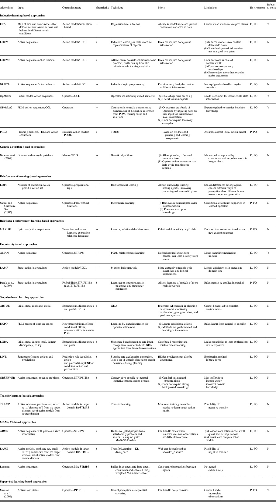
Learning systems can be also be characterized according to the sheer amount of detail represented in the output representation of the learnt model. This can range from a bare-bones STRIPS model produced in the output (Zhuo & Kambhampati, Reference Zhuo and Kambhampati2013), to PDDL models with quantifiers and logical implications (Zhuo et al., Reference Zhuo, Yang, Hu and Li2010), to PDDL models with static predicates (predicates existing implicitly in operator preconditions and never appearing in plans, e.g., Jilani et al., Reference Jilani, Crampton, Kitchin and Vallati2015). Granularity is used a criteria to classify the works summarized in the Table 3 based on the richness of the information learnt based on the amount of input provided.
State of the art planning algorithms

CNF = Conjunctive Normal Form; D=Deterministic; PO=Partially Observable; PDDL=Planning Domain Definition Language; OCL=Object-Centered Language; PDM=Partial Domain Model; TDIDT=Top-Down Induction of Decision Trees; P=Probabilistic; FO=Fully Observable; FOL=First-Order Logic; STRIPS=STanford Research Institute Problem Solver; PGM=Probabilistic Graphical Model; PDL=Prodigy Description Language; GDA=Goal Driven Autonomy; MAX-SAT=Maximum Satisfiability; KL=Kullback–Leibler; PPDDL=Probabilistic PDDL.
Granularity: +, high; i, intermediate; −, low.
4 Type of learning
This section sheds light on some classical learning techniques which have been around and in use for learning action models, as well as newer and interesting techniques which have emerged with recent advancements and the broadening spectrum of ML techniques. The algorithms described in this paper are further summarized in the form of Table 3. These tables provide a bird’s eye view of the key characteristics of each algorithm in terms of input provided, output produced, application environment, etc. These tables are described with the intent of serving someone who is new to the domain and is looking to situate their problem in the context of a previously done work.
4.1 Learning techniques based on availability of background knowledge
As discussed in Section 3.2.2, the learning techniques based on the absence or presence of BK are classified into inductive and analytical learning techniques, respectively.
4.1.1 Inductive learning
The learning system is fed with a hypothesis space
 $$H$$
and a set of traces
 $$T$$
. The desired output is a hypothesis from the space
 $$H$$
that is consistent with these traces (Zimmermann & Kambhampati, Reference Zimmerman and Kambhampati2003). Inductive techniques are useful because they can identify patterns and generalize over many examples in the absence of a domain model. One prominent inductive learning technique is that of regression tree learning. Regression trees are capable of predicting continuous variables and modeling noise in the data. In comparison to a decision tree which predicts along a category (i.e. class), a regression tree performs value prediction along the dependent dimension for all observations (Balac et al., Reference Balac, Gaines and Fisher2000).
The Planning, Execution and Learning Architecture system (Jiménez et al., Reference Jiménez, Fernández and Borrajo2008) performs the three functions suggested in its name to generate probabilistic rules from plan executions and compile them to refine its planning model. This is done by performing multiclass classification, which consists of using the Top-Down Induction of Decision Trees (Quinlan, Reference Quinlan1986) algorithm to find the smallest decision tree that fits a given data set. A decision tree is built from examples from which probabilities are captured to refine its initial model.
In Exploration, Regression tree induction and Action models (Balac et al., Reference Balac, Gaines and Fisher2000), a robot learns action models for its navigation under various terrain conditions. With each exploration step, the robot records the executed action, the current terrain conditions and positions before and after the action execution. When exploration is finished, the data are divided into groups based on action type and a regression tree induction algorithm is applied to the data for each action type. This algorithm then builds a regression tree representing the model and expected outcome of that particular action.
LOCM (Cresswell et al., Reference Cresswell, McCluskey and West2009, Reference Cresswell, McCluskey and West2013) uses an object-centered representation and learns a set of parameterized Finite State Machines (FSM), where each FSM represents pre and post-conditions of the domain operators (Jilani et al., Reference Jilani, Crampton, Kitchin and Vallati2014). A planning domain consists of sets (called sorts) of object instances, where each object behaves in the same way as any other object in its sort. LOCM first collects the set of all transitions in the example sequences. It then derives a set of state machines, each of which can be identified with a sort. It then performs inductive learning and identifies state parameters, providing correlations between the action0 parameters and state parameters occurring in the start/end states of transitions (Cresswell et al., Reference Cresswell, McCluskey and West2009, Reference Cresswell, McCluskey and West2013). The limitation of LOCM is that it provides a single state machine to represent each object, which is overcome by LOCM2 (Cresswell & Gregory, Reference Cresswell and Gregory2011).
LOCM2 (Cresswell & Gregory, Reference Cresswell and Gregory2011) is generalized and heuristic in nature to allow multiple state machines to represent a single object. This extends the coverage of domains for which a domain model can be learned. Unlike LOCM, LOCM2 constructs many possible solutions to the same problem. The heuristic is used to select a single solution from these possible solutions. This means that the learned models produce plans which are shorter than optimal solutions. Note that both systems gather only dynamic properties of a planning domain and not the static ones. This is a drawback as many systems use static predicates to contain the set of possible actions. This limitation is addressed by the NLOCM (Numeric LOCM) system.
NLOCM (Gregory & Lindsay, Reference Gregory and Lindsay2016) extends classical planningFootnote 1 to numerical planning, that is learns action costs in planning domains from state transition sequences using a constraint programming approach. It uses the LOCM2 and LOP systems as pre-processing steps. While the LOCM and LOCM2 algorithms only learn the dynamic aspects of the domain, the LOP system (Gregory & Cresswell, Reference Gregory and Cresswell2015) learns static relations. NLOCM extends the FSM of LOCM to an automata with numeric weights on the important features. A set of templates is defined for each operator which contributes to the action cost of that operator in the domain. The algorithm successively solves more and more complex template sets until a satisfying assignment which minimizes the complexity cost is found. These templates are used to find the valid cost models.
Opmaker (McCluskey et al., Reference McCluskey, Richardson and Simpson2002) is a mixed initiative tool to induce operators from action sequences, domain knowledge and user interaction. These operators are parameterized and hierarchical in nature. OCL is used to model the domain. For each action in the training solution sequence, it asks the user to input, if needed, the target state that each object would occupy after the action execution, thus creating its operator schema step-by-step. It is implemented inside a graphic tool called Graphical Interface for Planning with Objects, which facilitates user interaction, domain modeling and operator induction (McCluskey et al., Reference McCluskey, Richardson and Simpson2002; Jilani et al., Reference Jilani, Crampton, Kitchin and Vallati2014).
Opmaker2 (McCluskey et al., Reference McCluskey, Cresswell, Richardson and West2009) is an improvement over Opmaker such that it eliminates the dependency on the user for intermediate state information. After Opmaker2 automatically infers this intermediate state information, it proceeds in the same fashion as Opmaker and induces the same operators. The main advantage of Opmaker2 is that it computes its own intermediate states using a combination of heuristics and inference from the partial domain model (PDM), example sequences and solutions. In Opmaker2, the
 $$DetermineStates$$
procedure performs this function by tracking the changing states of each object referred to in the training example, taking advantage of the static and other information in the PDM. The output from
 $$DetermineStates$$
is, for each object, a map associating each object to a unique state value at each point in the training sequence. Once the map has been generated, the techniques of the original Opmaker algorithm are used to create an operator schema.
In Martínez et al. (Reference Martínez, Alenya, Torras, Ribeiro and Inoue2016), the authors learn a probabilistic model including exogenous effects (predicates not related to any action execution) from a set of state transitions. They use the Learning From Interpretation Transitions framework (Inoue et al., Reference Inoue, Ribeiro and Sakama2014) which uses ILP to induce a set of propositional rules that orchestrate the given input transitions. This is done by first transforming grounded to relational transitions, then relational transitions to probabilistic rules. Planning operators can be reconstructed from probabilistic rules. A score function evaluates the operators, and a heuristic search algorithm selects the set of operators that maximize the score.
4.1.2 Analytical learning
The learning system has at its disposal the same hypothesis space
 $$H$$
and traces as in the case of inductive learning but with an additional input: BK that can explain traces. The desired output is a hypothesis from the space
 $$H$$
that is consistent with both the traces and BK. Analytic learning relies on BK to analyze a given trace and identify its relevant features. Any system which relies on domain knowledge, predicate information or intermediate state information can be classified under this category. More details about analytic learning techniques can be found in (Zimmermann & Kambhampati, Reference Zimmerman and Kambhampati2003).
4.2 Genetic and evolutionary algorithm-based approaches
A series of approaches which use evolutionary algorithms to learn macro actions in the absence of any kind of additional knowledge may be classified under this category. An approach by (Newton et al., Reference Newton, Levine, Fox and Long2007) learns macro-actions given a domain and action sequences. It is generic in the sense that it does not require structural knowledge about the domain or the planner, but learns from plans generated for random planners and domains using a genetic algorithm.
Another approach by the same author (Newton & Levine, Reference Newton and Levine2010) learns macros as well as macro-sets (collection of macros which collectively perform well). In this work, once a macro is learned, it is tinkered with by adding, deleting and modifying existing and new actions in a bid to learn how the new macro-performs. In the first phase, only individual macros are learned using actions from generalized plans produced by solving input problems. In the second phase, macro-sets are learned using the macro pool obtained in the first phase, including only those that have fitness values greater than a certain minimum level.
In a third approach by the same author (Newton et al., Reference Newton, Levine, Fox and Long2008), non-observable macros, that is macros that are not observable from traces are learned. This is done with the intent of constructing a comprehensive macro-library for future reuse. Learning is based on an evolutionary algorithm. Evolutionary algorithms repeatedly generate new macros (in every epoch) from current individuals by using given genetic operators: only the individuals with the best fitness values survive through successive epochs. The fitness function is based on three measures:
 $$Cover,Score,Point$$
.
 $$Cover$$
evaluates the percentage of problems solved when the macro is used.
 $$Score$$
measures the time gained or lost over all the problems solved with the augmented domain compared to when they are solved using the original domain.
 $$Point$$
measures the percentage of problems solved with the augmented domain which take less or equal time compared to when they are solved using the original domain.
4.3 Reinforcement learning
Reinforcement learning (RL) is a special case of inductive learning, and more specifically characterizes a learning problem instead of a learning technique (Sutton & Barto, Reference Sutton and Barto1998). An RL problem is composed of three principal elements: (i) the goal an agent must achieve, (ii) a stochastic environment and (iii) actions an agent takes to modify the state of the environment (Sutton & Barto, Reference Sutton and Barto1998). RL takes place during the process of plan building. Through trial-and-error online traversal of states, an optimal policy (mapping from perceived states of the environment to actions to be taken when in those states) is found for achieving the agent’s goals (Zimmermann & Kambhampati, Reference Zimmerman and Kambhampati2003). The strength of RL lies in its ability to handle dynamic and stochastic environments where the domain model is either non-existent or incomplete. The benefits of an RL system are twofold: on one hand, it improves plan quality (the system progressively moves toward finding an optimal policy) and, on the other, it can learn the domain model. One of the major drawbacks of RL is that of generalization: in its bid to achieve domain-specific goals, it cannot gather general knowledge of the system dynamics, leading to a problem of generalization. Despite its drawbacks, RL played a major role in the success of real life systems such as the recent AlphaGo (Silver et al., Reference Silver, Huang, Maddison, Guez, Sifre, Van Den Driessche, Schrittwieser, Antonoglou, Panneershelvam, Lanctot and Dieleman2016). AlphaGo used policy gradient RL (policy represented by own function approximator) to optimize a deep convolutional neural network by simulating games of the network playing against previous versions of itself and rewarding itself for taking moves that gave it wins.
The Learning by Observation in Planning Environments (García-Martínez & Borrajo, Reference García-Martínez and Borrajo2000) system learned planning operators by observing the consequences of the execution of planned actions in the environment. In the beginning, the system is a blank slate and has no knowledge, it perceives the initial situation, and selects a random action to execute in the environment. It then loops by (1) executing an action, (2) perceiving the resulting situation of the action execution and its utility, (3) learning a model from this perception and (4) planning for further interaction with the environment. A global reinforcement mechanism either rewards or punishes operators based on their success in predicting the environment behavior. This is done by a virtual generalized Q table (associates each
 $$(s,a)$$
pair with an estimate of
 $$Q(s,a)$$
, where
 $$s$$
and
 $$a$$
are state and action, respectively, and
 $$Q(s,a)$$
is the expected reward for taking action
 $$a$$
in state
 $$s$$
).
In an approach by Safaei and Ghassem-Sani (Reference Safaei and Ghassem-Sani2007), probabilistic planning operators are learned in an incremental fashion. It has an integrated learning-planning system consisting of (i) an observation module for operator learning, (ii) an acting module for planning and (iii) a control center for generating goals to further test the algorithm. This control center also dynamically assigns the reward function.
4.3.1 Relational reinforcement learning
Relational reinforcement learning (RRL) is the combination between RL and inductive logic programming (Džeroski et al., Reference Džeroski, De Raedt and Driessens2001). Given a (i) possible state set
 $$S$$
, (ii) possible action set
 $$A$$
, (iii) state transition function
 $$\delta \,\colon\,S{\times}A\toS$$
, (iv) reward function
 $$r\,\colon\,S{\times}A\toS$$
, (v) BK and (vi) declarative bias for learning policy representations; the task is finding a policy
 $$\pi $$
for selecting actions
 $$\pi \,\colon\,S\toA$$
that maximizes the expected reward. RRL employs the Q-learning method (learns policies which are represented as value-assigned state-action pairs) using a relational regression tree. Due to the use of a more expressive relational language, RRL can be applied to a wider array of problems. It also allows the reuse of results of previous learning phases and their application to novel and more challenging situations.
MARLIE (Model-Assisted Reinforcement Learning in Expressive languages) is the first RRL system that learns a transition and reward function online (Croonenborghs et al., Reference Croonenborghs, Ramon, Blockeel and Bruynooghe2007). MARLIE builds probabilistic models accounting for the uncertainty of world dynamics. It uses the TG algorithm (Driessens et al., Reference Driessens, Ramon and Blockeel2001) to learn relational decision trees. The decision trees are not restructured on the appearance of new examples. However, their fully relational aspect allows them to be applicable to a wider range of problems.
IRALe (Incremental Relational Action Learning algorithm) (Rodrigues et al., Reference Rodrigues, Gérard, Rouveirol and Soldano2011) produces a STRIPS-like (see Table 1) action model consisting of a set of rules by combining RRL and active learning. At first, the action model is an empty rule-set. The interactions between the agent and the environment produce examples. In the event of a counter example (an example that contradicts the model), the example has to be revised by modifying or adding one or more rules. This contradiction is determined by matching operations performed between the rules and examples, and each identified counter-example leads to either a specialization or a generalization. The agent also performs active learning, that is, in every state it chooses an action that it expects to lead to a generalization of the model. IRALe is mainly bottom-up, and new opportunities for generalizing the model will decrease the number of examples required to converge to the correct model. It uses a formalism called Extended Deterministic STRIPS, which is more expressive than traditional STRIPS.
4.4 Uncertainty-based techniques
4.4.1 Markov logic networks
A Markov logic network (MLN) (Richardson & Domingos, Reference Richardson and Domingos2006) is a combination of first order logic and probabilistic graphical models (PGM). It is a first-order knowledge base consisting of weighted formulas, and can be equated to a template used to construct Markov networks. They have numerous advantages. From the probability point of view, MLNs provide a language scalable enough to specify very large Markov networks, and the ability to inject a comprehensive range of domain knowledge into them. From the first-order logic point of view, MLNs are equipped with the ability to soundly handle imperfect knowledge and uncertainty. For example, the Learning Action Models from Plan traces system (Zhuo et al., Reference Zhuo, Yang, Hu and Li2010) learns action models with quantifiers and logical implications using MLNs. First, the input plan traces (state–action interleavings) are encoded into propositional formulas (conjunction of ground literals) to store into a database as a collection of facts. These formulas are very close to PDDL (refer to Table 1) in terms of representation. Second, candidate formulas are generated according to the predicate lists and domain constraints. Third, a MLN uses the formulas generated in the above two steps to learn the corresponding weights of formulas and select the most likely subset from the candidate formula set. Finally, this subset is transformed into the final action models (Zhuo et al., Reference Zhuo, Yang, Hu and Li2010).
4.4.2 Noisy trace treatment approaches
As explained in Section 3.2.3, sensor miscalibration may cause introduce noise giving birth to uncertainty. For example, AMAN handles noise (Zhuo et al., Reference Zhuo, Nguyen and Kambhampati2013) by finding a domain model that best explains the observed noisy plan traces using a PGM-based approach. The only input to the learning phase are traces in the form of noisy action sequences. A PGM (graphical representation of dependence among random variables) is used to capture the relationship between the current state, correct action, observed action and the domain model. First, a set of all possible candidate models is generated. Then the observed noisy plan traces are used to predict the correct plan traces based on the PGM. Then, the correct plan traces are executed to calculate the reward of the predicted correct plan traces according to a predefined reward function. This reward function output is used to update the weights of the candidate models. The model with the highest weight is rendered as the model being searched for (Jilani et al., Reference Jilani, Crampton, Kitchin and Vallati2014).
In a series of works by Pasula et al., (Reference Pasula, Zettlemoyer and Kaelbling2004, Reference Pasula, Zettlemoyer and Kaelbling2007), Zettlemoyer et al. (Reference Zettlemoyer, Pasula and Kaelbling2005), the goal is to learn action models in noisy and stochastic domains. This is done by: (i) allowing rules to refer to objects not mentioned in the signature of the action. (ii) Relaxing the frame assumption (unspecified atoms in the operator’s effects remain unchanged) and allowing the existence of “noise-induced” changes in the world. (iii) Extending the language: introducing newer and more complex like existential quantification, universal quantification, counting and transitive closure. It allows to learn probabilistic rules which are affected by a factor of noise and include deictic references, thus are called Noisy Deictic Rules. Deictic references are used to identify objects, even those which are not directly affected by the mentioned predicates. The works conclude that the addition of noise and deictic references increases the quality of the learned rules.
4.5 Surprise-based learning
In a learning system, a surprise is produced if the latest prediction and the latest observation are considerably different (Ranasinghe & Shen, Reference Ranasinghe and Shen2008). Once an action is performed, the world state is sensed by a perceptor module which extracts sensor information. If the algorithm had made a prediction, it is verified by the surprise analyzer. If the prediction turns out incorrect, the model modifier adjusts the world model accordingly. Based on the updated model, the action selector will perform the next action so as to repeat the learning cycle. This notion of isolating faults is ideologically equivalent to the model-based diagnosis approaches to explain faults presented in De Jonge et al. (Reference De Jonge, Roos and Witteveen2009), Kalech (Reference Kalech2012), Micalizio and Torasso (Reference Micalizio and Torasso2014).
A series of approaches based on surprise-based learning (SBL) have used Goal-Driven Autonomy (GDA). GDA (Weber et al., Reference Weber, Mateas and Jhala2012) is a conceptual model for creating an autonomous agent that (i) monitors expectations during plan execution (ii) detects the occurrence of discrepancies, (iii) builds explanations and new goals to pursue in the case of failures. In order to identify when planning failures occur, a GDA agent requires the planning component to generate an expectation of world state after executing each action in the execution environment. The GDA model thus provides a framework for creating agents capable of responding to unforeseen failures during plan execution in complex environments.
FOOLMETWICE (Molineaux & Aha, Reference Molineaux and Aha2014) is a goal-oriented algorithm which learns from surprises. It tries to find inaccuracies in the environment model by attempting to explain all received observations. When a consistent explanation cannot be found, it infers that some unknown event happened that is not represented in the model. It then creates a model of the preconditions of these events by generalizing over the states that trigger them.
LIVE (Shen, Reference Shen1993) is a discrimination-based learning method that creates general rules by noticing the changes in the environment, then specifying the rules by explaining their failures in prediction. When a rule executes and the predicted outcome does not match the observation, LIVE explores and creates new sibling rules. These rules are usually created by comparing the difference between a successful previous execution and the current failed one. New rules can accordingly be made more specific/generic.
LGDA (Learning GDA) (Jaidee et al., Reference Jaidee, Muñoz-Avila and Aha2011) is a GDA algorithm that uses case-based reasoning to map state–action pairs to a distribution over expected states, and map goal-discrepancy pairs to a value distribution over discrepancy-resolution goals. It also uses RL to learn the expected values of the goals. It models goal formulation as an RL problem in which the value of a goal is estimated based on the expected future reward obtained on achieving it.
OBSERVER (Wang, Reference Wang1996) is an integrated learning, planning and execution system which incrementally learns planning operators. The learning module learns operator preconditions and effects by observing experts executing sample problems, then refining the operators collected from these observations. The operator preconditions are learned by creating and updating both the most specific and most general representations of the preconditions based on trace executions. Operator effects are learned by generalizing the delta-state (the difference between pre-state and post-state) from multiple observations. This learning mechanism adopted by OBSERVER can also be seen in many following works (Walsh & Littman, Reference Walsh and Littman2008; Stern & Brendan, Reference Stern and Brendan2017).
The EXPO (Gil, Reference Gil1992) system refines incomplete planning operators by a method called the operator refinement method. EXPO does this by generating plans and monitoring their execution to detect the difference between the predicted and observed state. EXPO then constructs a set of specific hypotheses to fix the detected differences. After heuristic filtration, each hypothesis is experimentally tested and a plan is constructed to achieve the required situation (Jiménez et al., Reference Jiménez, De La Rosa, Fernández, Fernández and Borrajo2012).
The ARTUE (Autonomous Response to Unexpected Events) system (Molineaux et al., Reference Molineaux, Klenk and Aha2010) dynamically reasons about the goals to pursue when encountered with unexpected environmental situations. It consists of four principal components. A Hierarchical Task Network planner reasons about exogenous events. A goal generation component reasons about and generates new goals. An explanation component reasons about hidden information in the environment. Finally, a goal management component manages and communicates the goals to the planner. ARTUE handles unexpected environmental changes by first explaining those changes, then generating new goals incorporating the explained knowledge about hidden environmental aspects.
4.6 Transfer learning
Transfer learning is the technique which, given a source task and target task, aims to extract the knowledge from the source task and apply it to the target task in a situation where the latter has fewer training data (Pan & Yang, Reference Pan and Yang2010). Most ML methods work well only under a common assumption: the training and test data are drawn from the same probability distribution. However, when the distribution changes, most models need to be reconstructed, trained and tested from scratch using data generated from the new probability distribution. In many real-world applications, it is expensive, if not impossible, to regenerate the needed training data for model reconstruction. In order to reduce the effort to regenerate the training data, the possibility of knowledge transfer between domains would be ideal. Transfer learning (Pan & Yang, Reference Pan and Yang2010) allows the domains, tasks, and probability distributions used in training and testing to be different. For example, we may find that learning to recognize apples might help to recognize oranges. Some characteristics of transfer learning systems include: the type of knowledge to be transfered, situation of transfer and technique of transfer. As far as type of knowledge goes, some knowledge is specific to individual domains, while other may be common between different domains such that it may help improve performance for the target domain. After discovering which knowledge can be transferred, learning algorithms need to be developed to perform the knowledge transfer. The situation of transfer is an important characteristic as while it is important to know the situation in which a transfer must occur, it is equally important to know the situations in which transfer must not occur. In some cases, when the source domain and target domain are not related to each other, thus a brute-force transfer may be highly unsuccessful. In the worst case, it may even degrade the performance of the target domain, a situation referred to as negative transfer (e.g. when an Indian or British tourist in Europe learns to drive on the left side of the road).
The advantages of using transfer learning are clear: a change of features, domains, tasks and probability distributions from the training to the testing phase does not require the underlying learning model to be rebuilt. The disadvantages are listed as follows:
∙ Most existing transfer learning algorithms assume that the source and target domains are related to each other in some sense. However, if the assumption does not hold, negative transfer may happen. In order to avoid negative transfer learning, measures to ascertain transferability between source domains and target domains needs to be studied. Based on this study of possible transferability, we can then select relevant source domains/tasks to extract knowledge for learning the target domains/tasks.
∙ Most existing transfer learning algorithms so far have focused on improving generalization across different distributions between source and target domains or tasks. In doing so, they assumed that the feature spaces between the source and target domains are the same. However, in many applications, we may wish to transfer knowledge across domains or tasks that have different feature spaces. This type of transfer learning is referred to as heterogeneous transfer learning, which remains a challenge yet to be overcome (Pan & Yang, Reference Pan and Yang2010).
A perfect example of transfer learning is the TRAMP (Transfer learning Action Models for Planning) system. TRAMP, given a set of traces in the target domain and expert-created domain models in the source domain, learns action models in the target domain by transferring knowledge from the source domain. TRAMP first encodes the input plan traces, which are state-action interleavings, into propositional formulas then as databases. Second, TRAMP encodes the action models from the source domains to a propositional formula set. Third, TRAMP generates a candidate formula set to structure the target action models, building mappings between the source and target domains by searching keywords of predicates and actions from the Web then calculating similarities of Web pages to bridge the gap between the two and transfer knowledge. Finally, TRAMP learns action models from the transferred knowledge with the help of MLNs (Zhuo & Yang, Reference Zhuo and Yang2014).
4.7 Maximum Satisfiability-based approaches
A weighted MAX-SAT (maximum satisfiability) problem can be stated as: given a collection
 $$C$$
of
 $$m$$
clauses
 $$(C_{1} ,...,C_{m} )$$
involving the disjunction of
 $$n$$
logical variables, with clause weights
 $$w_{i} $$
, find a truth assignment of the logical variables that maximizes the total weight of the satisfied clauses in
 $$C$$
(Zhuo & Yang, Reference Zhuo and Yang2014). Among works that use MAX-SAT, the learn action models with transferring knowledge from a related source domain via Web search system (Zhuo et al., Reference Zhuo, Muñoz-Avila and Yang2011) makes use of action models already created beforehand in other source domains, to help learn models in the target domain. The target domain and a related source domain are bridged by searching Web pages related to the two domains, and then building a mapping between them by means of a similarity function which calculates the similarity between their corresponding Web pages. The similarity is calculated using the Kullback–Leibler divergence. Based on the calculated similarity, a set of weighted constraints, called Web constraints, are built. Other constraints such as state, action and plan constraints, are also built from traces in the target domain. All the above constraints are solved using a weighted MAX-SAT solver, and target domain action models are reconstructed from the satisfied clauses.
The ARMS (Action-Relation Modeling System) (Yang et al., Reference Yang, Wu and Jiang2007) system learns action models from traces which consist of action sequences occasionally interleaved with intermediate states. The parsed predicates are encoded in the form of intra-operator constraints called information and action constraints respected by these predicates. Frequent action pairs in the traces are identified with the help of the apriori algorithm (Agrawal & Srikant, Reference Agrawal and Srikant1994), which are then used to obtain a set of intra-operator plan constraints. These constraints are then solved with the help of a satisfiability (SAT) solver. The constraints which amount to true are used to reconstruct the actions of the domain model. The process iterates until all actions are modeled.
The Refining Incomplete planning domain Models through plan traces system (Zhuo et al., Reference Zhuo, Nguyen and Kambhampati2013) enriches its partial model during the process of learning. It constructs sets of soft and hard constraints from incomplete models and plan traces. These constraints are again intra-operator and inter-operator ones that must be satisfied by atomic actions as well as macro-actions. The novelty of this approach is that it learns macro-actions as well. Macro-actions increase the accuracy of the incomplete model. These constraints are solved with the help of a SAT solver. The constraints which amount to true are used to obtain sets of macro-actions and refined action models.
The Lammas (Learning Models for Multi-Agent Systems) system (Zhuo et al., Reference Zhuo, Nguyen and Kambhampati2013) learns action models from input plan traces in the same lines of ARMS, however, extended to a multi-agent setting. Lammas also encodes the input plan traces as constraints which fall into one of the following three categories: (1) correctness constraints imposed on the relationship between actions in plan traces to ensure that causal links in the plan traces is not broken, (2) action constraints encoding the actions based on STRIPS semantics and (3) coordination constraints encoded from an Agent Interaction Graph describing inter-agent interactions. The learnt actions are represented in the MA-STRIPS language which is more adapted for a multi-agent setting (Brafman & Domshlak, Reference Brafman and Domshlak2008).
4.8 Supervised learning-based approaches
In Mourão et al. (Reference Mourão, Petrick and Steedman2008), the authors learn the effects of an agent’s actions given a set of actions and their preconditions, in a partially observable and noisy environment. The input to the learning mechanism uses a vector representation that encodes a description of the action being performed and the state at which the action is applied. The final input vector representing a particular action applied to a certain state has the form:
 $$(actions,object{\minus}independentproperties,object{\minus}dependentproperties)$$
. The output vector has the form:
 $$(object{\minus}independentproperties,object{\minus}dependentproperties)$$
. The task is to learn the associations between action-precondition pairs and their effects, that is, rules of the form
 $$(A,Pre(A)\toEff(A))$$
. The learning problem has a set of binary classification problems, and the perceptron is used as a classifier. The prediction consists of calculating the kernel matrix, and the kernel trick is used in the case of nonlinearly separable data (Mourão et al., Reference Mourão, Petrick and Steedman2008).
Another work by the same authors (Mourão et al., Reference Mourão, Petrick and Steedman2010) is based on the same lines, except that a voted kernel perceptron learning model with a Disjunctive Normal Form (DNF) kernel (
 $$K(x,y){\equals}2^{{same(x,y)}} $$
, where
 $$same(x,y)$$
is the number of bits with equal values in
 $$x$$
and
 $$y$$
) is used, allowing the perceptron to run over the entire space of possible rules (Sadohara et al., Reference Sadohara2001). Action and state information is encoded in a vector representation as input to the learning model, and resulting state changes are produced in the form of an output vector. A third approach by the same authors (Mourão et al., Reference Mourão, Zettlemoyer, Petrick and Steedman2012) decomposes the learning problem into two stages: learning implicit action models and progressively deriving explicit rules from the implicit models. Rules are extracted from classifiers based on the notion that more discriminative features will contribute more to the classifier’s objective function. The classifiers use the 3-DNF kernel.
A very recent work by the same authors (Mourão, Reference Mourão2014) learns probabilistic planning operators from noisy traces. While the precedent approaches find the most probable outcome, this approach emphasizes on generating alternately less probable outcomes from noisy traces. The rule fragments (partial precondition and single effect predicates) derived from classifiers that only contributed to the preconditions provide for a source of alternative effects for the planning operator. An alternative rule is created by reusing the precondition from the planning operator, and by one-by-one combining the effects of the rule fragments. Each new effect is accepted if the resulting rule gives better F-scores than the previous rule on the remaining training examples. Once all the rule fragments have been considered, we delete the training examples covered by the new rule as well as those fragments that contributed to the new rule. This process iterates until no further rules can be created.
5 Applications and open issues
This section is dedicated to highlight some of the feats of AP in terms of deployments in real-world applications serving actual needs. It then proceeds to account for some key issues which continue to plague the domain.
5.1 Applications of AP
Planning has found its place into an array of real-world applications which range from human multi-drones search-and-rescue missions (Bevacqua et al., Reference Bevacqua, Cacace, Finzi and Lippiello2015), single-operator multi-aircraft guidance (Strenzke & Schulte, Reference Strenzke and Schulte2011) to military evacuation operations (Muñoz-Avila et al., Reference Muñoz-Avila, Aha, Breslow and Nau1999).
Robotics is one of the most appealing application areas for AP. The fast-developing world of social robotics has cited planning and its ability to scale to real-world problems posed by robotics as a key issue to resolve. This is because most work done in AP is focused on action planning, whereas actions are not the only aspects that a robot reasons upon. Planning also needs to account for temporal, causal, resource and information dependencies between computational, perceptual, and actuation components (Di Rocco et al., Reference Di Rocco, Pecora and Saffiotti2013). This is increasingly falling into place. For example, the ROBIL team in the DARPA robotics challenge (www.darpa.mil/NewsEvents/Releases/2012/10/24.aspx) used hierarchical plans for runtime monitoring of resources (Cohen et al., Reference Cohen, Shimony and Weiss2015). The DARPA Grand Challenge is pivoted on path planning for autonomous vehicles, thus is beyond the scope of this paper. All in all, these works are gradual steps toward conceptualizing autonomous systems.
Achieving autonomous systems is one of the most prominent challenges of AP. AI planners have been successfully used in a wide range of applications with the intent of contributing toward the creation of autonomous systems. However, AP alone is not sufficient to achieve such kind of autonomy, and requires the amalgamation of perception, comprehension and projection capabilities in order to achieve contextual awareness leading to fully autonomous behavior (Endsley & Garland, Reference Endsley and Garland2000). From the perspective of AI planning and within the scope of this paper, we present a list of non-exhaustive guidelines that a robotic system can follow in order to be proclaimed autonomous:
∙ Capability of Autonomous Exploration and Conservative Planning: a robot must be capable of observing its surroundings using onboard sensors, selecting from a set of candidate locations, planning a trajectory and autonomously navigating to the selected location (Gregory et al., Reference Gregory, Fink, Rogers, Gupta and Crowley2016). Conservative planning is a method that seeks to exploit the classical planning framework, while simultaneously recognizing the opportunities (unexpected events). These opportunities are then used to increase the plan utility during its execution (Cashmore et al., Reference Cashmore, Fox, Long, Ridder and Magazzeni2016a).
∙ Persistent Autonomy: capable of planning long-term behavior and performing activity over extended periods of time without human intervention (Cashmore et al., Reference Cashmore, Fox, Long, Ridder and Magazzeni2016b).
∙ Interleaving with other tasks: this entails the combination of two types of planners: AI task planners that handle the high-level symbolic reasoning part and motion planners that plan the movements in space and check the geometrical feasibility of the plans output by the task planners (Ferrer-Mestres et al., Reference Ferrer-Mestres, Frances and Geffner2015). It also entails concurrent planning and execution abilities so that the robot can achieve the goal as quickly as possible.
AP techniques have also been used extensively in the field of space exploration, notably in satellite, rover and spacecraft missions. For example, the Deep Space One employed a constraint-based integrated temporal planner and resource scheduler which performed periodic planning to manage resources and develop plans to achieve goals in a timely manner (Muscettola et al., Reference Muscettola, Nayak, Pell and Williams1998; Pell et al., Reference Pell, Gat, Keesing, Muscettola and Smith1997).
5.2 Open issues
Despite the aforementioned joint advances in the fields of AP and ML, there remain some issues which continue to cloud the domain. Some of the key issues are highlighted and discussed below.
∙ Fully AP-boon or bane?: The necessity of fully AP can be debated in a twofold fashion:
− Is it rational to envision a fully automated learning-planning-execution system?: Despite the usage of the most comprehensive and state-of-the-art ML techniques, there is a certain amount of user-provided domain knowledge which cannot be discounted; especially bearing in mind the direct correlation between the speed of learning and the amount of domain knowledge furnished. Thus even the highest level of automation cannot weed out the need and advantages of human intervention.
− Is a fully automated system needed at all?: Even the most competent ML system is somewhat of questionable use if it is not designed to factor in human’s desire of being able to control its surroundings and automated systems. Modern day users, aware of the fact that an ideal system is difficult to envision, prefer a system that can not only be useful in a real-life situation, but can also be at the mercy of the user, such that the user gets autonomy over the representation mechanism, language, kind of traces, etc.
∙ Ignored aspects:
− Re-usable knowledge: The cross domain transfer of knowledge from an existing domain to enrich the model learning process in an alien domain (similar to the source domain) with few training examples, is an approach which has come into light recently with a series of works in transfer learning (Pan & Yang, Reference Pan and Yang2010).
− Learning during plan execution: this refers to a situation where the expected and obtained system state after an action execution are not in accord with each other. It arises due to a flawed domain theory. It has been a major topic of neglect owing to the fact that a flawed domain theory is somewhat of an alien concept in classical planning. This has, however, been a topic of greater attention given a flurry of approaches which have been pivoted on SBL (Ranasinghe & Shen, Reference Ranasinghe and Shen2008).
∙ Learning with the time dimension: Time plays an imperative role in most real-life domains. For example, each dialogue in a human–robot interaction is composed of an utterance further accompanied by gestural, body and eye movements; all of them interleaved in a narrow time frame. These interactions may thus be represented by a time sequence, with the intent of learning the underlying action model. Barring some initial works in this area, time remains an interesting dimension to explore (Guillame-Bert & Crowley, Reference Guillame-Bert and Crowley2012; Zhang et al., Reference Zhang, Sreedharan and Kambhampati2015).
∙ Direct re-applicability of learned model: Direct re-use of a learned model by a planner continues to remain a concern. A model that has been learned by applying ML techniques is more often than not incomplete, more concretely: inadept to be fed to a planner to directly generate plans. It needs to be retouched and fine tuned by a domain expert in order to be reusable. This marks a stark incapability of prominently used ML techniques to be comprehensive, leaving scope for more research.
∙ Extension of classical planning to a full scope domain: The applicability of the aforementioned approaches, most of which have been tested on highly simplified toy domains and not in real scenarios, remains an issue to be addressed. As mentioned in Section 2, classical planning is founded on restrictive assumptions and dwells in determinism. However, the real world is laced with unpredictability: a predicate might switch its value spontaneously, the world may have hidden variables, the exact impact of actions may be unpredictable and so on (Zimmermann & Kambhampati, Reference Zimmerman and Kambhampati2003). Thus, the application of a model learned on benchmark traces into the real world remains a point to ponder about. Barring a few works (Ortiz et al., Reference Ortiz, García-Olaya and Borrajo2013), a fair share of algorithms that treat noisy traces are learning on benchmark traces which they have been ‘self-adulterated’ to produce noisy ones. This can be seen as a means of a conscious steering of the learning algorithm toward a higher rate of learning, raising questions over their neutrality.
6 Conclusion
AP has been gaining steam ever since studies into human problem solving, operations research (primarily state space search) and theorem proving started gaining momentum. This is because the notion of a series of actions orchestrating the accomplishment of a goal is one that resonates among all these fields. However, depending on the domain characteristics, its constituent actions are difficult to quantify thus codify. Planners are now equipped with the capability to reverse engineer the signatures, preconditions and effects of the domain-applicable actions. This reverse engineering is achieved by capitalizing on several state-of-the-art and classical ML techniques. The article broadly classifies ML approaches based on several criteria, along with the merits and limitations of each approach. It then highlights some persisting open issues with the discussed approaches. It concludes that while a significant number of interesting techniques have been applied to highly controlled experimental setups and toy domains, their full-blown application to diverse and uncertain real-world scenarios remains a topic of further research.