3.1 Theory

We first write the solution to (1.1) using the Green’s function formulation. The streamwise and spanwise extents are taken to be infinite and the frame of reference is assumed to be stationary. We use a zero normal derivative of the pressure fluctuation as the boundary condition at the top and bottom walls. The Stokes component of pressure arising from the non-zero wall-normal derivative of wall-pressure fluctuation at the top and bottom wall has been shown to be negligible when compared to the rapid and slow terms for high Reynolds number flows (Hoyas & Jiménez Reference Hoyas and Jiménez2006; Gerolymos, Sénéchal & Vallet Reference Gerolymos, Sénéchal and Vallet2013). The wall-normal coordinates of the top and bottom wall are $y=+\unicode[STIX]{x1D6FF}$ and $y=-\unicode[STIX]{x1D6FF}$ respectively. The Fourier transform is defined as

(3.1a,b)$$\begin{eqnarray}g(t)=\int _{-\infty }^{\infty }{\hat{g}}(\unicode[STIX]{x1D714})\text{e}^{\text{i}\unicode[STIX]{x1D714}t}\,\text{d}\unicode[STIX]{x1D714};\quad {\hat{g}}(\unicode[STIX]{x1D714})={\displaystyle \frac{1}{2\unicode[STIX]{x03C0}}}\int _{-\infty }^{\infty }g(t)\text{e}^{-\text{i}\unicode[STIX]{x1D714}t}\,\text{dt},\end{eqnarray}$$

where ${\hat{g}}(\unicode[STIX]{x1D714})$ is the Fourier transform of $g(t)$. The pressure fluctuation

(3.2)$$\begin{eqnarray}\left.\begin{array}{@{}c@{}}p(x,y,z,t)=\displaystyle \iint _{-\infty }^{\infty }\hat{p}(k_{1},y,k_{3},t)\text{e}^{\text{i}(k_{1}x+k_{3}z)}\,\text{d}k_{1}\,\text{d}k_{3},\\ \hat{p}(k_{1},y,k_{3},t)=\displaystyle \int _{-\unicode[STIX]{x1D6FF}}^{+\unicode[STIX]{x1D6FF}}G(y,y^{\prime },k_{1},k_{3})\hat{f}(k_{1},y,k_{3},t)\,\text{d}y^{\prime },\\ \hat{f}(k_{1},y,k_{3},t)=\displaystyle {\displaystyle \frac{1}{(2\unicode[STIX]{x03C0})^{2}}}\iint _{-\infty }^{\infty }f(x,y,z,t)\text{e}^{-\text{i}(k_{1}x+k_{3}z)}\,\text{d}x\,\text{d}z,\end{array}\right\}\end{eqnarray}$$

where $f(x,y,z,t)$ is the right-hand side source term in the Poisson equation (equation (1.1)), $\hat{p}(k_{1},y,k_{3},t)$ and $\hat{f}(k_{1},y,k_{3},t)$ denote the Fourier transform in the spanwise and streamwise directions of $p(x,y,z,t)$ and $f(x,y,z,t)$ respectively, and the Fourier transform $\hat{p}(k_{1},y,k_{3},t)$ is defined similar to $\hat{f}(k_{1},y,k_{3},t)$ in the above equation. The Green’s function $G(y,y^{\prime },k_{1},k_{3})$ can be shown to be

(3.3)$$\begin{eqnarray}\left.\begin{array}{@{}c@{}}G(y,y^{\prime },k_{1},k_{3})=\left\{\begin{array}{@{}ll@{}}{\displaystyle \frac{\text{cosh}(k(y^{\prime }-\unicode[STIX]{x1D6FF}))\text{cosh}(k(y+\unicode[STIX]{x1D6FF}))}{2k\text{sinh}(k\unicode[STIX]{x1D6FF})\text{cosh}(k\unicode[STIX]{x1D6FF})}},\quad & y\leqslant y^{\prime },\\ {\displaystyle \frac{\text{cosh}(k(y^{\prime }+\unicode[STIX]{x1D6FF}))\text{cosh}(k(y-\unicode[STIX]{x1D6FF}))}{2k\text{sinh}(k\unicode[STIX]{x1D6FF})\text{cosh}(k\unicode[STIX]{x1D6FF})}},\quad & y>y^{\prime },\end{array}\right.\\ k=\sqrt{k_{1}^{2}+k_{3}^{2}},\end{array}\right\}\end{eqnarray}$$

for all combinations of $k_{1},k_{3}$ except when both $k_{1}=0$ and $k_{3}=0$, for which we can obtain

(3.4)$$\begin{eqnarray}G(y,y^{\prime },k_{1},k_{3})=\left\{\begin{array}{@{}ll@{}}{\textstyle \frac{1}{2}}(y-y^{\prime }),\quad & y\leqslant y^{\prime },\\ {\textstyle \frac{1}{2}}(y^{\prime }-y),\quad & y>y^{\prime }.\end{array}\right.\end{eqnarray}$$

In order to ensure uniqueness of the Green’s function when $k=0$, we have made use of the condition that the instantaneous average of the top and bottom wall-pressure fluctuation is zero. The above Green’s function has been previously used by Kim (Reference Kim1989) to obtain wall-pressure fluctuations from the Kim, Moin & Moser (Reference Kim, Moin and Moser1987) simulation.

The wall-pressure fluctuation of a point $(x,z)$ on the bottom wall is

(3.5)$$\begin{eqnarray}\displaystyle p(x,-\unicode[STIX]{x1D6FF},z,t) & = & \displaystyle \displaystyle \iint _{-\infty }^{\infty }p(k_{1},-\unicode[STIX]{x1D6FF},k_{3},t)\text{e}^{\text{i}(k_{1}x+k_{3}z)}\,\text{d}k_{1}\text{d}k_{3},\nonumber\\ \displaystyle & = & \displaystyle \displaystyle \iint _{-\infty }^{\infty }\int _{-\unicode[STIX]{x1D6FF}}^{+\unicode[STIX]{x1D6FF}}G(-\unicode[STIX]{x1D6FF},y,k_{1},k_{3})f(k_{1},y,k_{3},t)\,\text{d}y\text{e}^{\text{i}(k_{1}x+k_{3}z)}\,\text{d}k_{1}\,\text{d}k_{3},\nonumber\\ \displaystyle & = & \displaystyle \displaystyle \int _{-\unicode[STIX]{x1D6FF}}^{+\unicode[STIX]{x1D6FF}}\iint _{-\infty }^{\infty }G(-\unicode[STIX]{x1D6FF},y,k_{1},k_{3})f(k_{1},y,k_{3},t)\text{e}^{\text{i}(k_{1}x+k_{3}z)}\,\text{d}k_{1}\,\text{d}k_{3}\,\text{d}y,\nonumber\\ \displaystyle & = & \displaystyle \displaystyle \int _{-\unicode[STIX]{x1D6FF}}^{+\unicode[STIX]{x1D6FF}}f_{G}(x,y,z,t)\,\text{d}y,\end{eqnarray}$$

where $f_{G}(x,y,z,t)$ is termed the ‘net source’ because it includes contribution from all sources in a wall-parallel plane and the Green’s function. It includes the contribution from all streamwise and spanwise wavenumbers. The Green’s function essentially assigns a weight to each wavenumber $(k_{1},k_{3})$ component of the source in the wall-parallel plane. Note that the function $f_{G}(x,y,z,t)$ is homogeneous in the streamwise and spanwise directions.

In order to characterize the features of the net source function $f_{G}(x,y,z,t)$, the net source CSD $\unicode[STIX]{x1D6E4}(r,s,\unicode[STIX]{x1D714})$ is defined as

(3.6)$$\begin{eqnarray}\unicode[STIX]{x1D6E4}(r,s,\unicode[STIX]{x1D714})={\displaystyle \frac{1}{2\unicode[STIX]{x03C0}}}\int _{-\infty }^{\infty }\langle f_{G}^{\ast }(x,r,z,t)f_{G}(x,s,z,t+\unicode[STIX]{x1D70F})\rangle \text{e}^{-\text{i}\unicode[STIX]{x1D714}\unicode[STIX]{x1D70F}}\,\text{d}\unicode[STIX]{x1D70F}.\end{eqnarray}$$

It can be related to the five-dimensional CSD $\unicode[STIX]{x1D711}_{ff}(r,s,k_{1},k_{3},\unicode[STIX]{x1D714})$ of the pressure Poisson source terms as

(3.7)$$\begin{eqnarray}\unicode[STIX]{x1D6E4}(r,s,\unicode[STIX]{x1D714})=\iint _{-\infty }^{+\infty }G^{\ast }(0,r,\text{k}_{1},\text{k}_{3})G(0,s,\text{k}_{1},\text{k}_{3})\unicode[STIX]{x1D711}_{ff}(r,s,k_{1},k_{3},\unicode[STIX]{x1D714})\,\text{d}k_{1}\,\text{d}k_{3},\end{eqnarray}$$

where

(3.8)$$\begin{eqnarray}\displaystyle \unicode[STIX]{x1D711}_{ff}(r,s,k_{1},k_{3},\unicode[STIX]{x1D714}) & = & \displaystyle {\displaystyle \frac{1}{(2\unicode[STIX]{x03C0})^{3}}}\iiint _{-\infty }^{+\infty }\langle f^{\ast }(x,r,z,t)f(x+\unicode[STIX]{x1D709}_{1},s,z+\unicode[STIX]{x1D709}_{3},t+\unicode[STIX]{x1D70F})\rangle \nonumber\\ \displaystyle & & \displaystyle \times \,\text{e}^{-\text{i}(k_{1}\unicode[STIX]{x1D709}_{1}+k_{3}\unicode[STIX]{x1D709}_{3}+\unicode[STIX]{x1D714}\unicode[STIX]{x1D70F})}\,\text{d}\unicode[STIX]{x1D709}_{1}\,\text{d}\unicode[STIX]{x1D709}_{3}\,\text{d}\unicode[STIX]{x1D70F}.\end{eqnarray}$$

The PSD of the spatially homogeneous wall-pressure fluctuation $\unicode[STIX]{x1D719}_{pp}(\unicode[STIX]{x1D714})$ is related to the net source CSD.

(3.9)$$\begin{eqnarray}\unicode[STIX]{x1D719}_{pp}(\unicode[STIX]{x1D714})=\int _{-\unicode[STIX]{x1D6FF}}^{+\unicode[STIX]{x1D6FF}}\int _{-\unicode[STIX]{x1D6FF}}^{+\unicode[STIX]{x1D6FF}}\unicode[STIX]{x1D6E4}(r,s,\unicode[STIX]{x1D714})\,\text{d}r\,\text{d}s.\end{eqnarray}$$

In order to analyse the contribution from a particular wall-parallel plane at $y=r$, we include its cross-correlation with every other wall-normal location $y^{\prime }=s$ by integrating $\unicode[STIX]{x1D6E4}(r,s,\unicode[STIX]{x1D714})$ along $s$.

(3.10)$$\begin{eqnarray}\unicode[STIX]{x1D6F9}(r,\unicode[STIX]{x1D714})=\int _{-\unicode[STIX]{x1D6FF}}^{+\unicode[STIX]{x1D6FF}}\unicode[STIX]{x1D6E4}(r,s,\unicode[STIX]{x1D714})\,\text{d}s.\end{eqnarray}$$

The resulting function $\unicode[STIX]{x1D6F9}(r,\unicode[STIX]{x1D714})$ can be shown to be the CSD of the wall-pressure fluctuation and the net source at $r$, i.e.

(3.11)$$\begin{eqnarray}\unicode[STIX]{x1D6F9}(r,\unicode[STIX]{x1D714})={\displaystyle \frac{1}{2\unicode[STIX]{x03C0}}}\int _{-\infty }^{\infty }\langle f_{G}^{\ast }(x,r,z,t)p(x,-1,z,t+\unicode[STIX]{x1D70F})\rangle \text{e}^{-\text{i}\unicode[STIX]{x1D714}\unicode[STIX]{x1D70F}}\,\text{d}\unicode[STIX]{x1D70F}.\end{eqnarray}$$

We will call $\unicode[STIX]{x1D6F9}(r,\unicode[STIX]{x1D714})$ the wall-pressure fluctuation – net source CSD. The wall-pressure PSD can be expressed in terms of $\unicode[STIX]{x1D6F9}(r,\unicode[STIX]{x1D714})$.

(3.12)$$\begin{eqnarray}\unicode[STIX]{x1D719}_{pp}(\unicode[STIX]{x1D714})=\int _{-\unicode[STIX]{x1D6FF}}^{+\unicode[STIX]{x1D6FF}}\unicode[STIX]{x1D6F9}(r,\unicode[STIX]{x1D714})\,\text{d}r.\end{eqnarray}$$

Next, we identify decorrelated features in the dataset that contribute the most to the wall-pressure PSD using $\unicode[STIX]{x1D6E4}(r,s,\unicode[STIX]{x1D714})$. To accomplish this, we use the Poisson inner product defined in (3.16) to enforce the orthonormality of the eigenfunctions instead of the commonly used $L^{2}$ inner product. We decompose $\unicode[STIX]{x1D6E4}(r,s,\unicode[STIX]{x1D714})$ as

(3.13)$$\begin{eqnarray}\unicode[STIX]{x1D6E4}(r,s,\unicode[STIX]{x1D714})=\mathop{\sum }_{i=1}^{\infty }\unicode[STIX]{x1D706}_{i}(\unicode[STIX]{x1D714})\unicode[STIX]{x1D6F7}_{i}(r,\unicode[STIX]{x1D714})\unicode[STIX]{x1D6F7}_{i}^{\ast }(s,\unicode[STIX]{x1D714}),\end{eqnarray}$$

where $\{\unicode[STIX]{x1D706}_{i}(\unicode[STIX]{x1D714}),\unicode[STIX]{x1D6F7}_{i}(r,\unicode[STIX]{x1D714})\}_{i=1}^{\infty }$ are the spectral POD eigenvalue and mode pairs. The mode $\unicode[STIX]{x1D6F7}_{i}(r,\unicode[STIX]{x1D714})$ relates to the eigenfunction $\bar{\unicode[STIX]{x1D6F7}}_{i}(r,\unicode[STIX]{x1D714})$ of $\unicode[STIX]{x1D6E4}(r,s,\unicode[STIX]{x1D714})$ through the relation

(3.14)$$\begin{eqnarray}\unicode[STIX]{x1D6F7}_{i}(r,\unicode[STIX]{x1D714})=\left(-(1-\unicode[STIX]{x1D6FD}){\displaystyle \frac{\unicode[STIX]{x2202}^{2}}{\unicode[STIX]{x2202}y^{2}}}+\unicode[STIX]{x1D6FD}\right)\bar{\unicode[STIX]{x1D6F7}}_{i}(r,\unicode[STIX]{x1D714}),\end{eqnarray}$$

where $\unicode[STIX]{x1D6FD}$ is a real number satisfying $0<\unicode[STIX]{x1D6FD}\leqslant 1$ and the eigenfunctions are assumed to satisfy zero Neumann boundary conditions $\bar{\unicode[STIX]{x1D6F7}}_{i}(r,\unicode[STIX]{x1D714})$ at $r=-\unicode[STIX]{x1D6FF}$ and $r=+\unicode[STIX]{x1D6FF}$. The eigenvalue problem for $\bar{\unicode[STIX]{x1D6F7}}_{i}(r,\unicode[STIX]{x1D714})$ and $\unicode[STIX]{x1D706}_{i}(\unicode[STIX]{x1D714})$ is

(3.15)$$\begin{eqnarray}\int _{-\unicode[STIX]{x1D6FF}}^{+\unicode[STIX]{x1D6FF}}\unicode[STIX]{x1D6E4}(r,s,\unicode[STIX]{x1D714})\bar{\unicode[STIX]{x1D6F7}}_{i}(s,\unicode[STIX]{x1D714})\,\text{d}s=\unicode[STIX]{x1D706}_{i}(\unicode[STIX]{x1D714})\left(-(1-\unicode[STIX]{x1D6FD}){\displaystyle \frac{\unicode[STIX]{x2202}^{2}}{\unicode[STIX]{x2202}y^{2}}}+\unicode[STIX]{x1D6FD}\right)\bar{\unicode[STIX]{x1D6F7}}_{i}(r,\unicode[STIX]{x1D714}).\end{eqnarray}$$

The spectral POD eigenvalues are arranged in decreasing order. The eigenfunctions $\bar{\unicode[STIX]{x1D6F7}_{i}}(r,\unicode[STIX]{x1D714})$ satisfy the orthonormality condition

(3.16)$$\begin{eqnarray}\left.\begin{array}{@{}c@{}}=\displaystyle \int _{-\unicode[STIX]{x1D6FF}}^{+\unicode[STIX]{x1D6FF}}\bar{\unicode[STIX]{x1D6F7}}_{i}^{\ast }(r,\unicode[STIX]{x1D714})\left(-(1-\unicode[STIX]{x1D6FD}){\displaystyle \frac{\unicode[STIX]{x2202}^{2}}{\unicode[STIX]{x2202}y^{2}}}+\unicode[STIX]{x1D6FD}\right)\bar{\unicode[STIX]{x1D6F7}}_{j}(r,\unicode[STIX]{x1D714})\,\text{d}r\\ =\unicode[STIX]{x1D6FF}_{ij},\end{array}\right\}\end{eqnarray}$$

where $\unicode[STIX]{x1D6FF}_{ij}$ is the Kronecker delta. We will call the inner product above ‘the Poisson inner product’ because the kernel $(-(1-\unicode[STIX]{x1D6FD})(\unicode[STIX]{x2202}^{2}/\unicode[STIX]{x2202}y^{2})+\unicode[STIX]{x1D6FD})$ can be related to the Poisson equation. If we choose $\unicode[STIX]{x1D6FD}=1$, then the Poisson inner product is the standard $L^{2}$ inner product.

The contribution of each spectral POD mode to wall-pressure PSD can be obtained by integrating equation (3.13) in $r$ and $s$,

(3.17a,b)$$\begin{eqnarray}\unicode[STIX]{x1D719}_{pp}(\unicode[STIX]{x1D714})=\mathop{\sum }_{i=1}^{\infty }\unicode[STIX]{x1D6FE}_{i}(\unicode[STIX]{x1D714});\quad \unicode[STIX]{x1D6FE}_{i}(\unicode[STIX]{x1D714})=\unicode[STIX]{x1D706}_{i}(\unicode[STIX]{x1D714})\left|\int _{-\unicode[STIX]{x1D6FF}}^{+\unicode[STIX]{x1D6FF}}\unicode[STIX]{x1D6F7}_{i}(r,\unicode[STIX]{x1D714})\,\text{d}r\right|^{2};\quad i=1,\ldots ,\infty .\end{eqnarray}$$

In the above equation, the wall-pressure PSD is expressed as sum of positive contributions $\{\unicode[STIX]{x1D6FE}_{i}(\unicode[STIX]{x1D714})\}_{i=1}^{\infty }$ from each spectral POD mode. We will use the quantities $\{\unicode[STIX]{x1D6FE}_{i}(\unicode[STIX]{x1D714})\}_{i=1}^{\infty }$ to identify the spectral POD modes that are the dominant contributors to wall-pressure PSD.

The spectral POD modes and eigenvalues depend on the parameter $\unicode[STIX]{x1D6FD}$. For a chosen value of $\unicode[STIX]{x1D6FD}$, we will have the corresponding set of spectral POD modes $\{\unicode[STIX]{x1D6F7}_{i}(y,\unicode[STIX]{x1D714})\}_{i=1}^{\infty }$ and eigenvalues $\{\unicode[STIX]{x1D706}_{i}(\unicode[STIX]{x1D714})\}_{i=1}^{\infty }$. However, irrespective of the chosen $\unicode[STIX]{x1D6FD}$, the component of the net source Fourier transform ($\hat{f}_{G}(x,y,z,\unicode[STIX]{x1D714})$) along the spectral POD modes will be decorrelated, i.e.

(3.18)$$\begin{eqnarray}\left.\begin{array}{@{}c@{}}\displaystyle f_{G}(x,y,z,t)=\int _{-\infty }^{+\infty }\hat{f}_{G}(x,y,z,\unicode[STIX]{x1D714})\text{e}^{\text{i}\unicode[STIX]{x1D714}t}\,\text{d}\unicode[STIX]{x1D714},\\ \displaystyle \hat{f}_{G}(x,y,z,\unicode[STIX]{x1D714})=\mathop{\sum }_{j=1}^{\infty }\unicode[STIX]{x1D6FC}_{j}(x,z,\unicode[STIX]{x1D714})\unicode[STIX]{x1D6F7}_{j}^{\ast }(y,\unicode[STIX]{x1D714}),\\ \langle \unicode[STIX]{x1D6FC}_{i}(x,z,\unicode[STIX]{x1D714})\unicode[STIX]{x1D6FC}_{j}^{\ast }(x,z,\unicode[STIX]{x1D714}_{o})\rangle =\unicode[STIX]{x1D706}_{i}(\unicode[STIX]{x1D714})\unicode[STIX]{x1D6FF}_{ij}\unicode[STIX]{x1D6FF}(\unicode[STIX]{x1D714}-\unicode[STIX]{x1D714}_{o}),\end{array}\right\}\end{eqnarray}$$

where $\{\unicode[STIX]{x1D6FC}_{j}(x,z,\unicode[STIX]{x1D714})\}_{j=1}^{\infty }$ are the coefficients, $\langle \cdot \rangle$ denotes ensemble average and $\unicode[STIX]{x1D6FF}$ is the Dirac delta function.

On the other hand, choosing the $L^{2}$ inner product ($\unicode[STIX]{x1D6FD}=1$) to enforce the orthonormality of the modes will also optimally decompose the wall-normal integral of the PSD $\unicode[STIX]{x1D6E4}(r,r,\unicode[STIX]{x1D714})$. Substituting $s=r$ in (3.13) and integrating in $r$, we obtain

(3.19)$$\begin{eqnarray}\left.\begin{array}{@{}c@{}}\displaystyle \unicode[STIX]{x1D6E4}(r,r,\unicode[STIX]{x1D714})=\mathop{\sum }_{j=1}^{\infty }\unicode[STIX]{x1D706}_{j}(\unicode[STIX]{x1D714})|\unicode[STIX]{x1D6F7}_{i}(r,\unicode[STIX]{x1D714})|^{2},\\ \displaystyle \int _{-\unicode[STIX]{x1D6FF}}^{+\unicode[STIX]{x1D6FF}}\unicode[STIX]{x1D6E4}(r,r,\unicode[STIX]{x1D714})\,\text{d}r=\mathop{\sum }_{j=1}^{\infty }\unicode[STIX]{x1D706}_{j}(\unicode[STIX]{x1D714}).\end{array}\right\}\end{eqnarray}$$

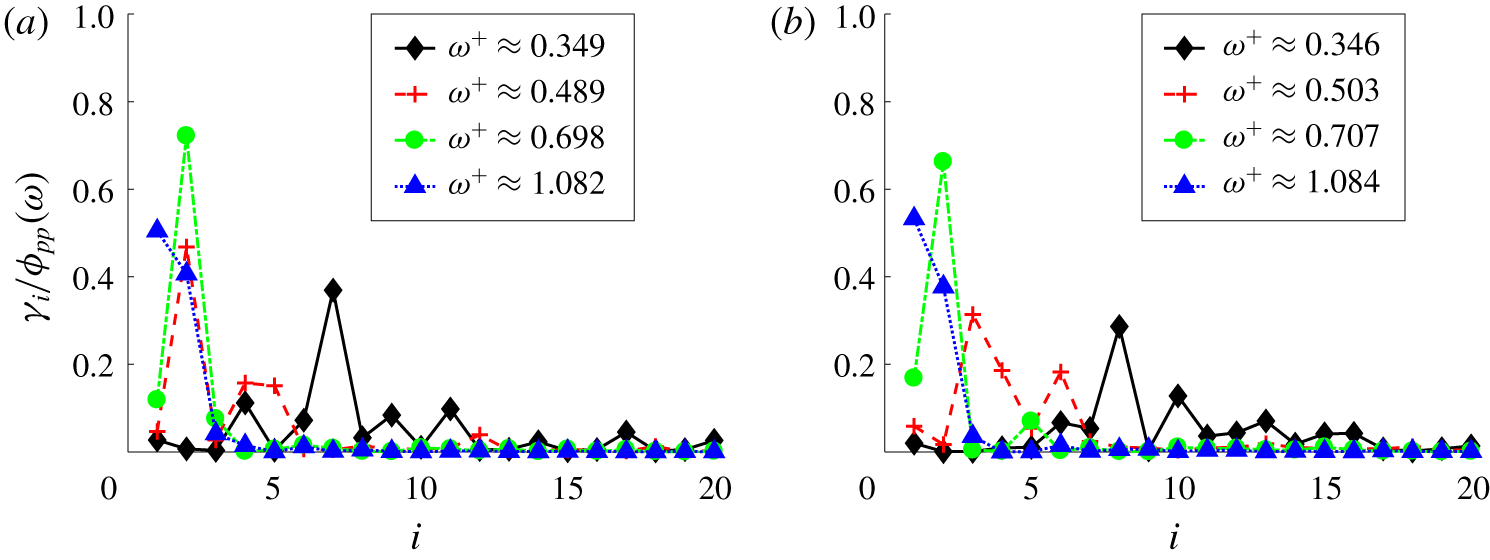
However, the dominant spectral POD modes obtained with the $L^{2}$ inner product do not necessarily isolate the main contribution to the wall-pressure PSD. i.e. the value of $\unicode[STIX]{x1D6FE}_{i}(\unicode[STIX]{x1D714})$. That is, the wall-pressure PSD can be distributed over a large number of modes that each individually contribute a small fraction. This makes it difficult to identify the few dominant decorrelated source patterns. Further, the single dominant wall-pressure mode (mode with largest $\unicode[STIX]{x1D6FE}_{i}(\unicode[STIX]{x1D714})$) does not necessarily contain any useful information about the source because it contributes only a small fraction to the wall-pressure PSD. This was observed at low frequencies (see figure 16).

Our goal is to identify useful decorrelated features of the wall-pressure source, not to optimally decompose the integrated net source PSD (as done by the $L^{2}$ inner product). Therefore, we use the parameter $\unicode[STIX]{x1D6FD}$ to our advantage and select a suitable value for $\unicode[STIX]{x1D6FD}$.

For $0<\unicode[STIX]{x1D6FD}<1$, it can be shown that the Poisson inner product optimally decomposes $\iint _{-\unicode[STIX]{x1D6FF}}^{+\unicode[STIX]{x1D6FF}}G(s,r,\unicode[STIX]{x1D6FD}/(1-\unicode[STIX]{x1D6FD}),0)/(1-\unicode[STIX]{x1D6FD})\unicode[STIX]{x1D6E4}(r,s,\unicode[STIX]{x1D714})\,\text{d}r\,\text{d}s$ into the sum of spectral POD eigenvalues,

(3.20)$$\begin{eqnarray}\iint _{-\unicode[STIX]{x1D6FF}}^{+\unicode[STIX]{x1D6FF}}{\displaystyle \frac{G\left(s,r,{\displaystyle \frac{\unicode[STIX]{x1D6FD}}{1-\unicode[STIX]{x1D6FD}}},0\right)}{1-\unicode[STIX]{x1D6FD}}}\unicode[STIX]{x1D6E4}(r,s,\unicode[STIX]{x1D714})\,\text{d}r\,\text{d}s=\mathop{\sum }_{j=1}^{\infty }\unicode[STIX]{x1D706}_{j}(\unicode[STIX]{x1D714}),\end{eqnarray}$$

where the Green’s function $G$ is given in (3.3). We can observe that as $\unicode[STIX]{x1D6FD}$ approaches $0$, the Green’s function $G(r,s,\unicode[STIX]{x1D6FD}/(1-\unicode[STIX]{x1D6FD}),0)$ becomes flatter and approaches a function that is constant in $r$ and $s$. Thus, the left-hand side in the above equation approaches the wall-pressure PSD $\unicode[STIX]{x1D719}_{pp}(\unicode[STIX]{x1D714})=\iint _{-1}^{+1}\unicode[STIX]{x1D6E4}(r,s,\unicode[STIX]{x1D714})\,\text{d}r\,\text{d}s$ (up to a scaling). As we decrease $\unicode[STIX]{x1D6FD}$, we can therefore expect the dominant spectral POD modes to be the dominant contributors to wall-pressure PSD. Therefore, the Poisson inner product in (3.16) identifies the few dominant features of wall-pressure sources that are decorrelated.

The Poisson inner product defined in (3.16) does not fall into the category presented by Towne et al. (Reference Towne, Schmidt and Colonius2018). They required the eigenfunctions to be orthonormal in a weighted $L^{2}$ inner product. Here, we use the Poisson inner product (3.16) that has a symmetric positive definite kernel.

The set of spectral POD modes obtained with any $\unicode[STIX]{x1D6FD}$ is complete. Therefore, we can relate the POD modes obtained with two different values of $\unicode[STIX]{x1D6FD}$ to each other through a linear transformation. That is, if $\{\hat{\unicode[STIX]{x1D6F7}}_{i}(y,\unicode[STIX]{x1D714})\}_{i=1}^{\infty }$ and $\{\tilde{\unicode[STIX]{x1D6F7}}_{i}(y,\unicode[STIX]{x1D714})\}_{i=1}^{\infty }$ are the two sets of spectral POD modes obtained with two different values of $\unicode[STIX]{x1D6FD}$, then

(3.21)$$\begin{eqnarray}\hat{\unicode[STIX]{x1D6F7}}_{i}(y,\unicode[STIX]{x1D714})=\mathop{\sum }_{j}C_{ij}^{\ast }(\unicode[STIX]{x1D714})\tilde{\unicode[STIX]{x1D6F7}}_{j}(y,\unicode[STIX]{x1D714}),\end{eqnarray}$$

where the matrix $C(\unicode[STIX]{x1D714})=[C_{ij}(\unicode[STIX]{x1D714})]$ is the linear transformation. Further, we show in appendix B that the linear transformation $C(\unicode[STIX]{x1D714})$ is indeed orthogonal with an appropriate row scaling, i.e.

(3.22)$$\begin{eqnarray}(\hat{\unicode[STIX]{x1D6EC}}^{1/2}(\unicode[STIX]{x1D714})C(\unicode[STIX]{x1D714}))^{H}\hat{\unicode[STIX]{x1D6EC}}^{1/2}(\unicode[STIX]{x1D714})C(\unicode[STIX]{x1D714})=\tilde{\unicode[STIX]{x1D6EC}}(\unicode[STIX]{x1D714}),\end{eqnarray}$$

where $\hat{\unicode[STIX]{x1D6EC}}(\unicode[STIX]{x1D714})$ and $\tilde{\unicode[STIX]{x1D6EC}}(\unicode[STIX]{x1D714})$ are the diagonal matrices of eigenvalues of the set of modes $\{\hat{\unicode[STIX]{x1D6F7}}_{i}(y,\unicode[STIX]{x1D714})\}_{i=1}^{\infty }$ and $\{\tilde{\unicode[STIX]{x1D6F7}}_{i}(y,\unicode[STIX]{x1D714})\}_{i=1}^{\infty }$, respectively.

We can show that

(3.23)$$\begin{eqnarray}\left|\int _{-\unicode[STIX]{x1D6FF}}^{+\unicode[STIX]{x1D6FF}}\unicode[STIX]{x1D6F7}_{i}(y,\unicode[STIX]{x1D714})\,\text{d}y\right|=\int _{-\unicode[STIX]{x1D6FF}}^{+\unicode[STIX]{x1D6FF}}|\unicode[STIX]{x1D6F7}_{i}(y,\unicode[STIX]{x1D714})|\cos (\angle \unicode[STIX]{x1D6F7}_{i}(y,\unicode[STIX]{x1D714})-\angle \unicode[STIX]{x1D6F7}_{i}^{n}(\unicode[STIX]{x1D714}))\,\text{d}y,\end{eqnarray}$$

where $\angle \unicode[STIX]{x1D6F7}_{i}^{n}(\unicode[STIX]{x1D714})=\angle (\int _{-\unicode[STIX]{x1D6FF}}^{+\unicode[STIX]{x1D6FF}}\unicode[STIX]{x1D6F7}_{i}(y,\unicode[STIX]{x1D714})\,\text{d}y)$ and $\angle$ denotes the phase of the complex number that follows it. Using (3.23) in (3.17), we obtain

(3.24)$$\begin{eqnarray}\unicode[STIX]{x1D6FE}_{i}(\unicode[STIX]{x1D714})=\unicode[STIX]{x1D706}_{i}(\unicode[STIX]{x1D714})\left(\int _{-\unicode[STIX]{x1D6FF}}^{+\unicode[STIX]{x1D6FF}}|\unicode[STIX]{x1D6F7}_{i}(r,\unicode[STIX]{x1D714})|\cos (\angle \unicode[STIX]{x1D6F7}_{i}(r,\unicode[STIX]{x1D714})-\angle \unicode[STIX]{x1D6F7}_{i}^{n}(\unicode[STIX]{x1D714}))\,\text{d}r\right)^{2};\quad i=1,\ldots ,\infty .\end{eqnarray}$$

From the above equation, we can observe that the eigenvalue, magnitude and phase of the spectral POD mode, all play a role in determining its contribution to wall-pressure PSD. Sources contained in wall-normal regions where the phase is in the range $|\angle \unicode[STIX]{x1D6F7}_{i}(y,\unicode[STIX]{x1D714})-\angle \unicode[STIX]{x1D6F7}_{i}^{n}(\unicode[STIX]{x1D714})|<\unicode[STIX]{x03C0}/2$ undergo destructive interference with the sources contained in the region where $\unicode[STIX]{x03C0}/2<|\angle \unicode[STIX]{x1D6F7}_{i}(y,\unicode[STIX]{x1D714})-\angle \unicode[STIX]{x1D6F7}_{i}^{n}(\unicode[STIX]{x1D714})|<\unicode[STIX]{x03C0}$. Therefore, the interference of the sources from different wall-normal regions represented by a spectral POD mode plays a role in determining the net contribution to wall-pressure PSD from the mode.

3.2 Implementation

The five-dimensional CSD $\unicode[STIX]{x1D711}_{ff}(r,s,k_{1},k_{3},\unicode[STIX]{x1D714})$ defined in (3.8) contains all pertinent information on velocity field sources from cross-correlation of two wall-normal locations. However, computing the function is extremely memory intensive. For the $Re_{\unicode[STIX]{x1D70F}}=400$ case, assuming 2000 frequencies, we would need ${\approx}$1220 TB to store $\unicode[STIX]{x1D711}_{ff}$. We use a streaming parallel implementation procedure to compute the net source CSD $\unicode[STIX]{x1D6E4}(r,s,\unicode[STIX]{x1D714})$ that makes the computation feasible.

The source term in (1.1) is computed and stored from the DNS. The stored data are divided into multiple chunks to compute the ensemble average in (3.8). For a given chunk, the source terms are first converted to stationary frame of reference and then Fourier transformed in $x$, $z$ and $t$. The Fourier transforms are then used to update the net source CSD. Details of the parallel implementation are provided in appendix A.

A total of 16 000 time steps are used to obtain the net source CSD $\unicode[STIX]{x1D6E4}(r,s,\unicode[STIX]{x1D714})$ for both $Re_{\unicode[STIX]{x1D70F}}$. We sample the data every time step. The number of time steps in each chunk is 2000 and 50 % overlap is used in time to increase statistical convergence. The frequency resolution of the analysis is $\unicode[STIX]{x0394}\unicode[STIX]{x1D714}\unicode[STIX]{x1D6FF}/u_{\unicode[STIX]{x1D70F}}=2\unicode[STIX]{x03C0}$.

Figure 1.

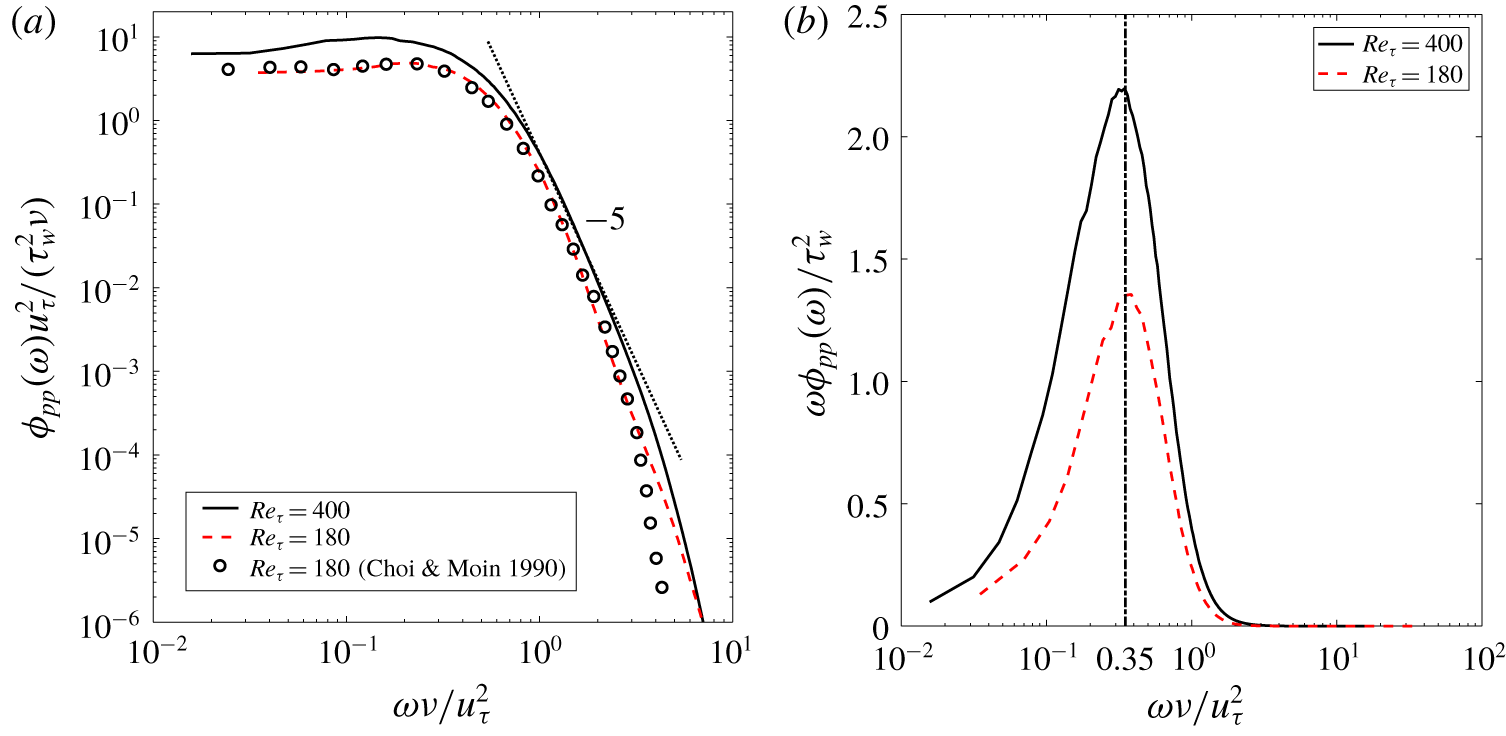
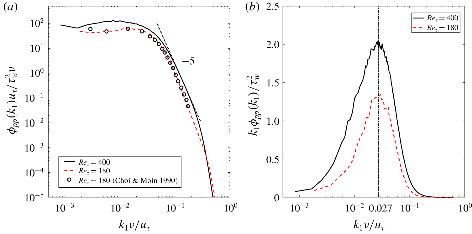
Wall-pressure fluctuation power spectra in (a) inner units and (b) premultiplied form with inner units on $x$-axis.

Figure 2.

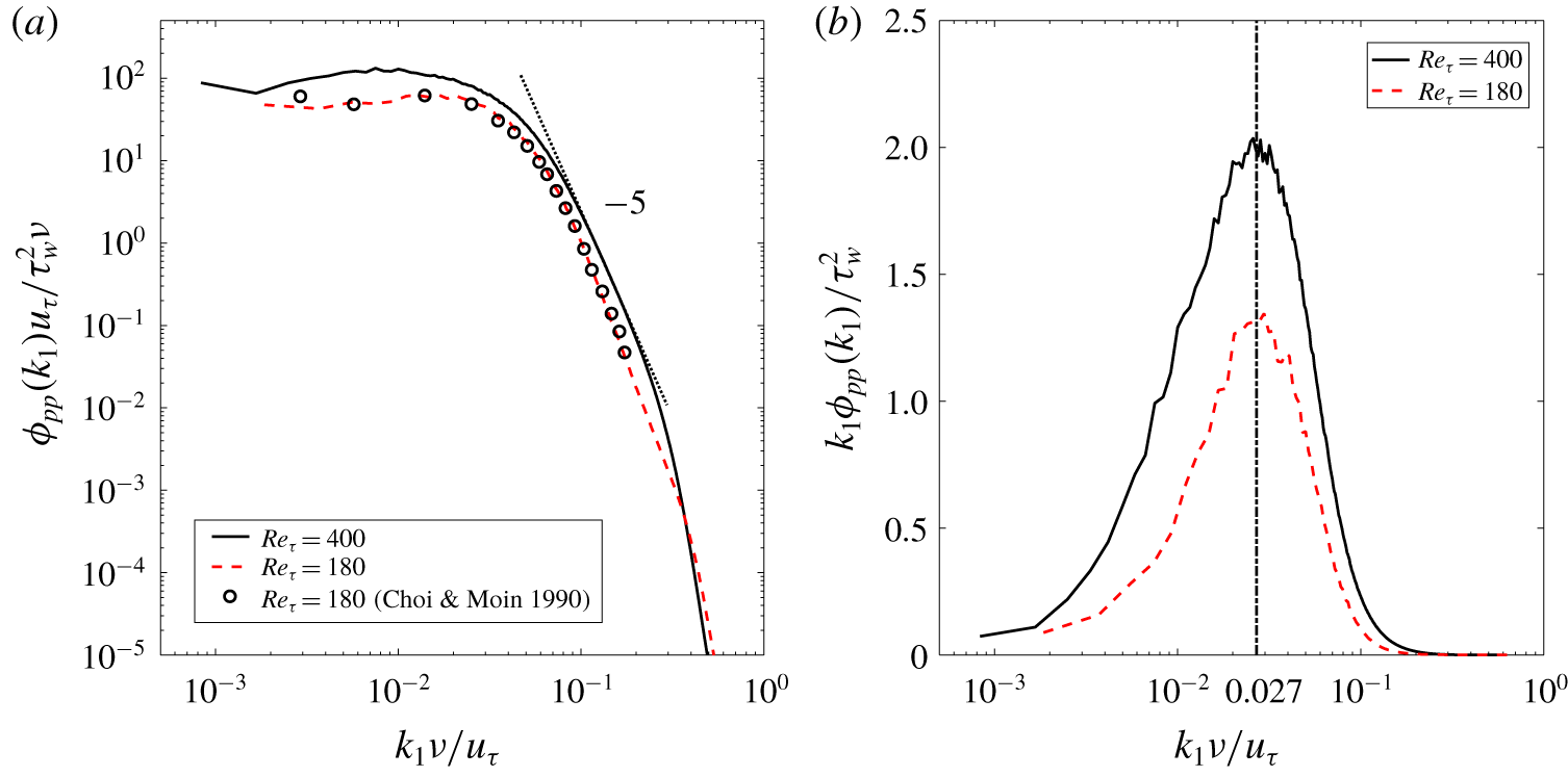
Wall-pressure fluctuation streamwise wavenumber spectra in (a) inner units and (b) premultiplied form with inner units on $x$-axis.

4.1 DNS wall-pressure fluctuations

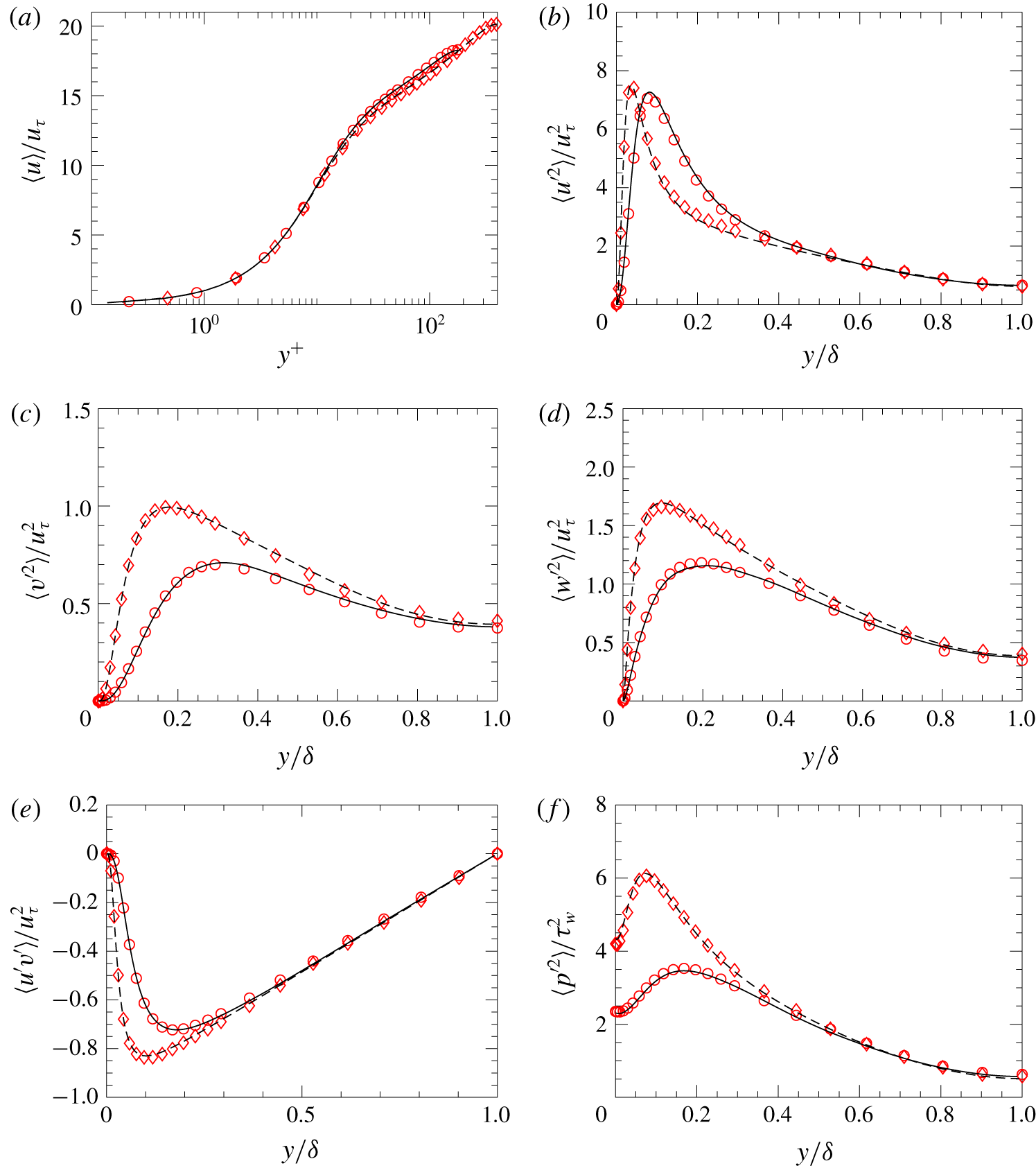
The one-sided PSD of the obtained $Re_{\unicode[STIX]{x1D70F}}=180$ and 400 wall-pressure fluctuations scaled with inner variables is shown in figure 1(a). The streamwise wavenumber spectra of the fluctuations at the two $Re_{\unicode[STIX]{x1D70F}}$ are shown in figure 2(a). Both the PSD and wavenumber spectra at $Re_{\unicode[STIX]{x1D70F}}=180$ agree well with the results of Choi & Moin (Reference Choi and Moin1990). The high-frequency region with $\unicode[STIX]{x1D714}^{+}=\unicode[STIX]{x1D714}\unicode[STIX]{x1D708}/u_{\unicode[STIX]{x1D70F}}^{2}>1$, shows a small region of $-5$ decay for the higher Reynolds number ($Re_{\unicode[STIX]{x1D70F}}=400$). The high-wavenumber region of the wavenumber spectra plotted in figure 2(a) also shows a small region of $-5$ decay in the region $k_{1}^{+}=k_{1}\unicode[STIX]{x1D708}/u_{\unicode[STIX]{x1D70F}}>0.1$, for the $Re_{\unicode[STIX]{x1D70F}}=400$ case. The premultiplied power spectra plotted in figure 1(b) for both $Re_{\unicode[STIX]{x1D70F}}$ show a peak at $\unicode[STIX]{x1D714}_{p}^{+}=0.35$. This peak at the same frequency has been previously observed by Hu et al. (Reference Hu, Morfey and Sandham2006) for $Re_{\unicode[STIX]{x1D70F}}$ up to 1440. Similar to the power spectra, the premultiplied streamwise wavenumber spectra in figure 2(b) also show a peak at $k_{1}^{+}=k_{1}\unicode[STIX]{x1D708}/u_{\unicode[STIX]{x1D70F}}$ at $k_{p}^{+}=0.027$. This peak has also been previously observed by Panton et al. (Reference Panton, Lee and Moser2017) for $Re_{\unicode[STIX]{x1D70F}}$ over the range 180–5000. The wall-pressure fluctuation PSD computed from the net source CSD using (3.9) agrees with that obtained directly from the solver (figure 1a) for both $Re_{\unicode[STIX]{x1D70F}}$ (not shown). We will investigate the distribution of the net sources that give rise to this premultiplied PSD peak in the next section.

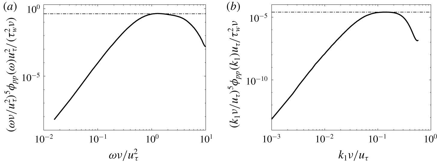
To identify the range of $-5$ decay in the power and streamwise wavenumber spectrum, we plot the diagnostic functions $(\unicode[STIX]{x1D714}\unicode[STIX]{x1D708}/u_{\unicode[STIX]{x1D70F}}^{2})^{5}\unicode[STIX]{x1D719}_{pp}(\unicode[STIX]{x1D714})u_{\unicode[STIX]{x1D70F}}^{2}/(\unicode[STIX]{x1D70F}_{w}^{2}\unicode[STIX]{x1D708})$ and $(k_{1}\unicode[STIX]{x1D708}/u_{\unicode[STIX]{x1D70F}})^{5}\unicode[STIX]{x1D719}_{pp}(k_{1})u_{\unicode[STIX]{x1D70F}}/(\unicode[STIX]{x1D70F}_{w}^{2}\unicode[STIX]{x1D708})$ in figures 3(a) and 3(b), respectively. The function is constant in the range of $-5$ slope. The diagnostic function does not return a significant range of frequency and wavenumbers that show $-5$ decay. We observe a constant value (indicated by the dashed-dotted horizontal line) for only a very small range of frequencies and wavenumbers. To observe the decay in a significant range, we require higher Reynolds numbers.

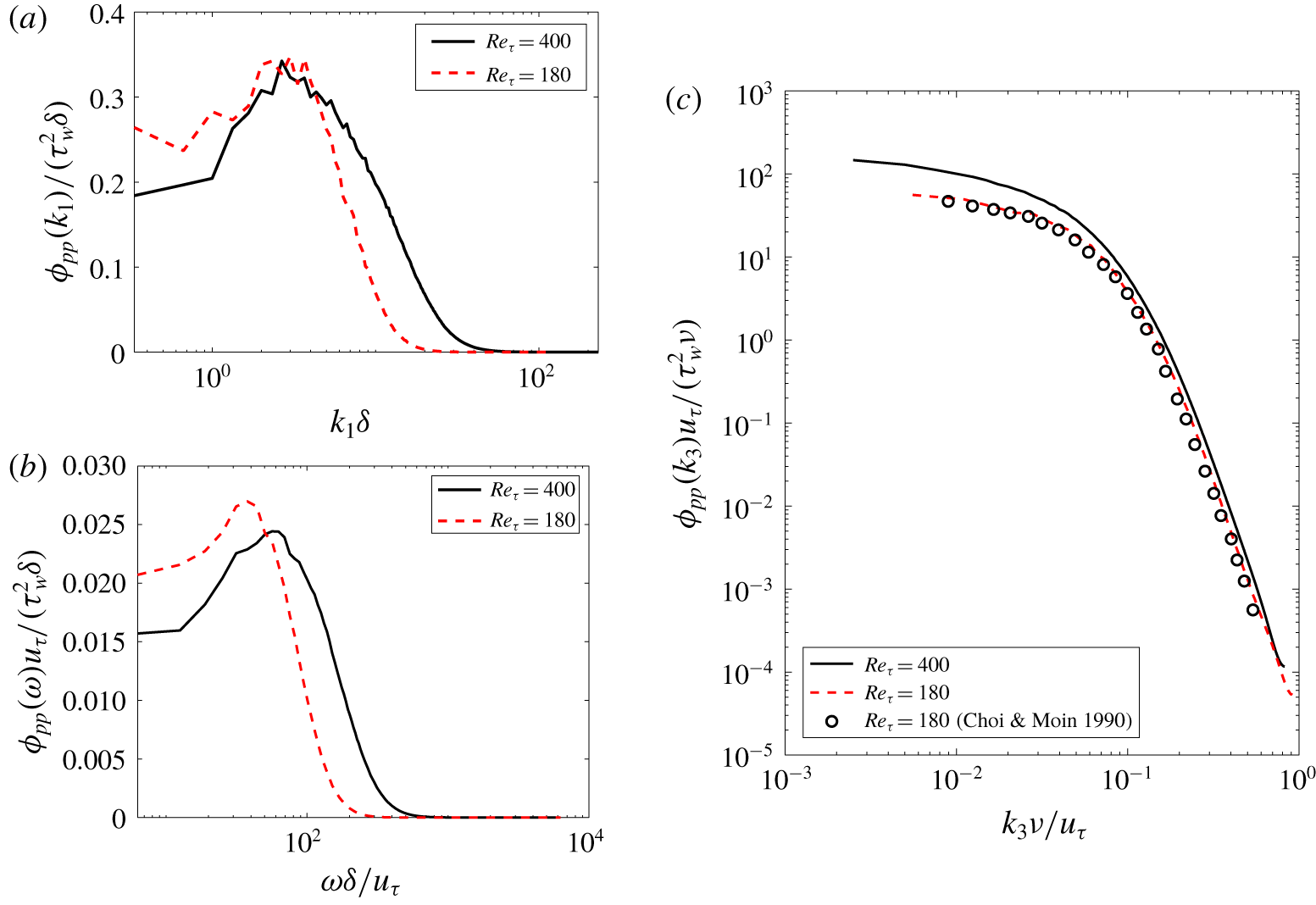
The wall-pressure wavenumber spectra show a low-wavenumber peak around $k_{1}\unicode[STIX]{x1D6FF}\approx 3$ for both $Re_{\unicode[STIX]{x1D70F}}=180$ and 400, respectively, when the $y$-axis is plotted in linear coordinates (figure 4a). This corresponds to streamwise wavelengths $\unicode[STIX]{x1D706}_{1}/\unicode[STIX]{x1D6FF}$ of ${\sim}2$. Such low-wavenumber peaks in the range $k_{x}\unicode[STIX]{x1D6FF}\approx 2.5{-}3.4$ ($\unicode[STIX]{x1D706}_{x}/\unicode[STIX]{x1D6FF}\approx 1.8{-}2.4$) have been previously observed by Abe et al. (Reference Abe, Matsuo and Kawamura2005) and Panton et al. (Reference Panton, Lee and Moser2017) in a turbulent channel for friction Reynolds numbers ranging from 180 to 5000. We observe the corresponding low-frequency peak in the wall-pressure PSD at $\unicode[STIX]{x1D714}\unicode[STIX]{x1D6FF}/u_{\unicode[STIX]{x1D70F}}=37.6$ and 50.2 for $Re_{\unicode[STIX]{x1D70F}}=180$ and 400, respectively (shown in figure 4b). Later, we identify the decorrelated fluid sources responsible for this low-frequency peak in the PSD using spectral POD and relate this to the observations of Abe et al. (Reference Abe, Matsuo and Kawamura2005).

Figure 4(c) shows the spanwise wavenumber spectrum of the wall-pressure fluctuations in inner units. The spectrum at $Re_{\unicode[STIX]{x1D70F}}=180$ agrees well with Choi & Moin (Reference Choi and Moin1990). Therefore, the spanwise resolution is sufficient enough to resolve the fine scale spanwise features of wall-pressure fluctuations.

Figure 3.

Diagnostic function to verify region of $-5$ slope in the $Re_{\unicode[STIX]{x1D70F}}=400$ (a) power and (b) streamwise wavenumber spectrum. The dashed-dotted horizontal lines in (a) and (b) indicate constant values of 0.42 and $2.53\times 10^{-5}$, respectively.

Figure 4.

(a) Wall-pressure fluctuation streamwise wavenumber spectrum with linear $y$-axis. (b) Wall-pressure fluctuation PSD with linear $y$-axis. (c) Wall-pressure fluctuation spanwise wavenumber spectrum in inner units.

Figure 5.

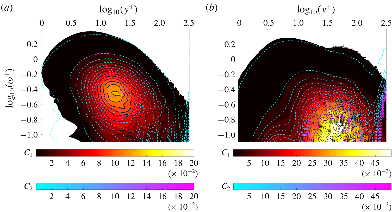
(a) Real part of premultiplied wall-pressure fluctuation – net source CSD ($y^{+}\unicode[STIX]{x1D714}^{+}Re(\unicode[STIX]{x1D6F9}(y^{+},\unicode[STIX]{x1D714}^{+}))/\langle p^{2}\rangle$) for $Re_{\unicode[STIX]{x1D70F}}=400$ (black solid lines with filled contours with colour map $C_{1}$) and 180 (line contours with colour map $C_{2}$). Contour lines are 20 equally spaced values between $4\times 10^{-4}$ and $2\times 10^{-1}$. (b) Premultiplied net source PSD $(y^{+}\unicode[STIX]{x1D714}^{+}\unicode[STIX]{x1D6E4}(y^{+},y^{+},\unicode[STIX]{x1D714}^{+})/\langle \unicode[STIX]{x1D6E4}^{2}\rangle )$ for $Re_{\unicode[STIX]{x1D70F}}=400$ (black solid lines with filled contours with colour map $C_{1}$) and 180 (line contours with colour map $C_{2}$). Contour lines are 20 equally spaced values between $4\times 10^{-5}$ and $5\times 10^{-2}$.

4.2 Wall-pressure source distribution analysis

The wall-parallel plane that contributes the most to the wall-pressure PSD can be determined from the real part of the wall-pressure fluctuation – net source CSD $\unicode[STIX]{x1D6F9}(y^{+},\unicode[STIX]{x1D714}^{+})$ (defined in § 3.1). Figure 5(a) shows the wall-pressure fluctuation – net source CSD in premultiplied form normalized by the root mean square (r.m.s.) of the wall-pressure fluctuations ($y^{+}\unicode[STIX]{x1D714}^{+}Re(\unicode[STIX]{x1D6F9}^{+}(y^{+},\unicode[STIX]{x1D714}^{+}))/\langle p^{2}\rangle ^{+}$); $y^{+}$ is the distance from the wall in viscous units. The coordinates $(\unicode[STIX]{x1D714}_{p}^{+},y_{p}^{+})$ of the peak value in the contours are $(0.35,16.5)$ and $(0.35,18.4)$ for $Re_{\unicode[STIX]{x1D70F}}=180$ and $400$, respectively. The frequency coordinate of the peak in the contour levels ($\unicode[STIX]{x1D714}^{+}=0.35$) is the same as the premultiplied power spectrum peak location shown in figure 1(b). Therefore, the corresponding wall-normal coordinate yields the location of the wall-parallel plane that contributes the most to the premultiplied power spectrum peak. Specifically, it is the cross-correlation with this dominant plane that contributes the most. This coincidence is not surprising since integrating figure 5(a) in the wall-normal direction yields figure 1(b) (normalized by $\langle p^{2}\rangle$). The wall-normal coordinate of the peak indicates that it is the correlations with the buffer region that contribute the most to the wall-pressure PSD at the Reynolds numbers considered.

Even though the peak location differs slightly in inner units for the two $Re_{\unicode[STIX]{x1D70F}}$, the main implication of this result is that the peak lies in the buffer region. Further, we cannot expect the same location of the peak for both $Re_{\unicode[STIX]{x1D70F}}$. This is because the real part of the peak wall-pressure fluctuation – net source CSD includes the contribution from the correlations with the rest of the channel (since $\unicode[STIX]{x1D6F9}(y_{p}^{+},\unicode[STIX]{x1D714})=\int _{-\unicode[STIX]{x1D6FF}}^{+\unicode[STIX]{x1D6FF}}\unicode[STIX]{x1D6E4}(y_{p}^{+},y^{\prime },\unicode[STIX]{x1D714})\,\text{d}y^{\prime }$) and not just the inner layer. Therefore, the peak need not necessarily scale in inner units. We believe that changing the Reynolds number would not affect this main finding. We expect the peak value of wall-pressure fluctuation – net source CSD to still occur in the buffer layer.

The phase difference between the wall-pressure and the dominant net source obtained from the argument of $\unicode[STIX]{x1D6F9}(y_{p}^{+},\unicode[STIX]{x1D714}_{p}^{+})$ is $0.013\unicode[STIX]{x03C0}$ and $0.016\unicode[STIX]{x03C0}$ for $Re_{\unicode[STIX]{x1D70F}}=180$ and 400 respectively, is very small. Hence, the dominant net sources and the wall-pressure fluctuation are in phase with each other. The contour levels of the normalized wall-pressure fluctuation – net source CSD plotted in figure 5(a) almost overlap in the range $\unicode[STIX]{x1D714}^{+}>0.3\sim 10^{-0.5}$. This indicates that the high-frequency contribution to the r.m.s. scales in inner units. However, in the near-wall region ($y^{+}<10$), the overlap in the contours is observed for a much larger frequency range $\unicode[STIX]{x1D714}^{+}>0.16\sim 10^{-0.8}$. This implies that for most of the frequency range, the contribution to wall-pressure PSD from the near-wall region scales in inner units.

Next, we investigate whether the net source PSD can be used to infer the location of the dominant source of wall-pressure fluctuation instead of the wall-pressure fluctuation – net source CSD. Figure 5(b) shows the contours of the premultiplied net source PSD $\unicode[STIX]{x1D6E4}(y^{+},y^{+},\unicode[STIX]{x1D714}^{+})$ in fractional form for both $Re_{\unicode[STIX]{x1D70F}}$. The main contribution to the net source PSD is seen to be from the region around $y^{+}\approx 30$ and at frequencies much lower than $\unicode[STIX]{x1D714}^{+}\approx 0.35$. There is no signature of the distinct premultiplied peak observed in figure 5(a). From visual inspection at low frequencies ($\unicode[STIX]{x1D714}^{+}<1$), the shape of the contours in figure 5(b) do not have similar shape to those in figure 5(a). 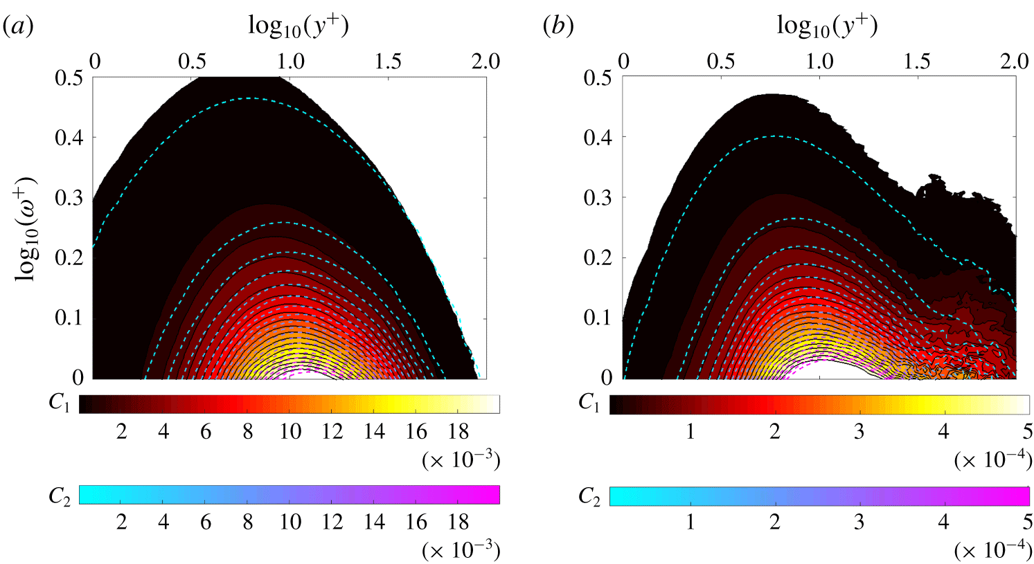However, at high frequencies $\unicode[STIX]{x1D714}^{+}>1$, we observe from figure 6(a,b) that the contour shapes near the wall ($y^{+}<30$) are almost identical. 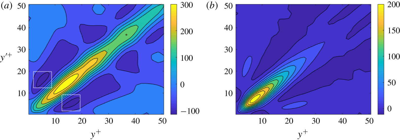Therefore, the net source PSD $\unicode[STIX]{x1D6E4}(y^{+},y^{+},\unicode[STIX]{x1D714}^{+})$ is a good proxy for wall-pressure fluctuation – net source CSD $\unicode[STIX]{x1D6F9}(y^{+},\unicode[STIX]{x1D714}^{+})$ at high frequencies to obtain the pattern of the net sources. The reason for this behaviour can be understood from the near-wall contours of the real part of the net source CSD shown in figure 7. Figures 7(a) and 7(b) show the contours at frequencies $\unicode[STIX]{x1D714}^{+}=0.35$ and $\unicode[STIX]{x1D714}^{+}=1$, respectively, for $Re_{\unicode[STIX]{x1D70F}}=180$. Clearly, the low-frequency ($\unicode[STIX]{x1D714}^{+}=0.35$) contours show a large negatively cross-correlated region around $(y^{+},{y^{\prime }}^{+})=(5,15)$ (shown by white boxes). These dominant negative regions found at low frequencies contribute to the wall-pressure fluctuation – net source CSD (3.10) leading to different shapes compared to the net source PSD. However, such negative regions are not present at the higher frequency $\unicode[STIX]{x1D714}^{+}=1$. Therefore, the wall-pressure fluctuation – net source CSD and the net source CSD have similar shapes near to the wall at high frequencies.

Figure 6.

(a) Real part of the high-frequency premultiplied wall-pressure fluctuation – net source CSD ($y^{+}\unicode[STIX]{x1D714}^{+}Re(\unicode[STIX]{x1D6F9}(y^{+},\unicode[STIX]{x1D714}^{+}))/\langle p^{2}\rangle$) for $Re_{\unicode[STIX]{x1D70F}}=400$ (black solid lines with filled contours with colour map $C_{1}$) and 180 (line contours with colour map $C_{2}$). Contour lines are 20 equally spaced values between $4\times 10^{-5}$ and $2\times 10^{-2}$. (b) High-frequency premultiplied fractional net source power spectral density $y^{+}\unicode[STIX]{x1D714}^{+}\unicode[STIX]{x1D6E4}(y^{+},y^{+},\unicode[STIX]{x1D714}^{+})/\langle \unicode[STIX]{x1D6E4}^{2}\rangle$ for $Re_{\unicode[STIX]{x1D70F}}=400$ (black solid lines with filled contours with colour map $C_{1}$) and 180 (line contours with colour map $C_{2}$). Contour lines are 20 equally spaced values between $4\times 10^{-6}$ and $2\times 10^{-2}$.

Figure 7.

Real part of $\unicode[STIX]{x1D6E4}(r,s,\unicode[STIX]{x1D714})$ (normalized by $\unicode[STIX]{x1D719}_{pp}(\unicode[STIX]{x1D714})$) at (a) $\unicode[STIX]{x1D714}^{+}\approx 0.35$ and (b) $\unicode[STIX]{x1D714}^{+}\approx 1$ for $Re_{\unicode[STIX]{x1D70F}}=180$.

Figure 8.

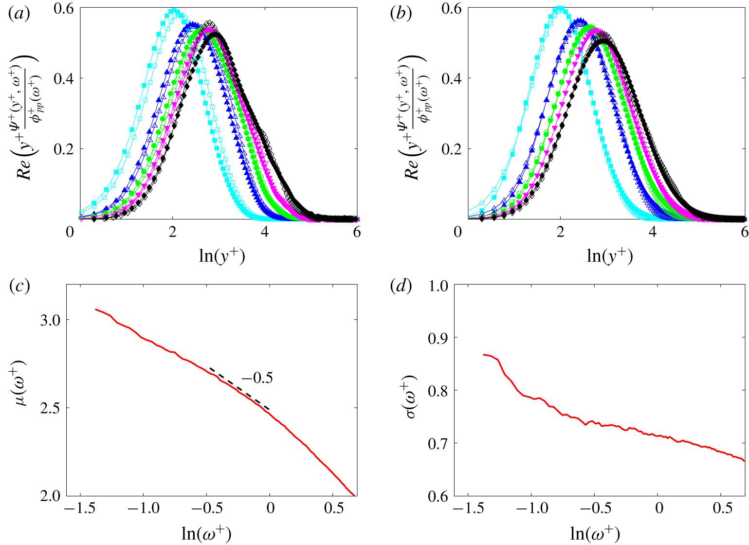
(a) Premultiplied wall-pressure fluctuation – net source CSD ($y^{+}\unicode[STIX]{x1D6F9}^{+}(y^{+},\unicode[STIX]{x1D714}^{+})/\unicode[STIX]{x1D719}_{pp}^{+}(\unicode[STIX]{x1D714}^{+})$) at different frequencies for $Re_{\unicode[STIX]{x1D70F}}=180$ (empty markers) and 400 (filled markers). (b) Comparison of fitted log-normal Gaussians (filled markers) to the wall-pressure fluctuation – net source for $Re_{\unicode[STIX]{x1D70F}}=400$ (empty markers). (c) Variation of mean $\unicode[STIX]{x1D707}(\unicode[STIX]{x1D714}^{+})$ and (d) standard deviation $\unicode[STIX]{x1D70E}(\unicode[STIX]{x1D714}^{+})$ of the fitted log-normal profile for $Re_{\unicode[STIX]{x1D70F}}=400$. ♢, ♦: $\unicode[STIX]{x1D714}^{+}\approx 0.35$, ▿, ▾: $\unicode[STIX]{x1D714}^{+}\approx 0.5$, ○, ●: $\unicode[STIX]{x1D714}^{+}\approx 0.7$, ▵, ▴: $\unicode[STIX]{x1D714}^{+}\approx 1$, ▫, ▪: $\unicode[STIX]{x1D714}^{+}\approx 2$.

The wall-pressure fluctuation – net source CSD (normalized with wall-pressure PSD) is plotted in premultiplied form for selected frequencies between $\unicode[STIX]{x1D714}^{+}=0.35$ and $\unicode[STIX]{x1D714}^{+}=2$ in figure 8(a). Due to the normalization, each profile has unit area under it. From the figure, we can observe that the curves for $Re_{\unicode[STIX]{x1D70F}}=180$ and 400 are very close to each other for the different frequencies plotted. Further, visual inspection shows that we can model the profiles using log-normal function in $y^{+}$. Therefore, normalized log-normal profiles of the form

(4.1)$$\begin{eqnarray}f(y^{+},\unicode[STIX]{x1D714}^{+})={\displaystyle \frac{1}{\unicode[STIX]{x1D70E}(\unicode[STIX]{x1D714}^{+})\sqrt{2\unicode[STIX]{x03C0}}}}\exp \left(-\left({\displaystyle \frac{\ln (y^{+})-\unicode[STIX]{x1D707}(\unicode[STIX]{x1D714}^{+})}{\sqrt{2}\unicode[STIX]{x1D70E}(\unicode[STIX]{x1D714}^{+})}}\right)^{2}\right)\end{eqnarray}$$

are fitted to the $Re_{\unicode[STIX]{x1D70F}}=400$ data for different $\unicode[STIX]{x1D714}^{+}$ using a nonlinear least squares fit and plotted in figure 8(b).

The mean and standard deviation of the fitted log-normal curves characterize the location and the width of the dominant net source respectively as a function of frequency. The correlation between the planes contained in this width have a sizeable contribution to wall-pressure PSD. Figures 8(c) and 8(d) show the mean ($\unicode[STIX]{x1D707}(\unicode[STIX]{x1D714}^{+})$) and standard deviation ($\unicode[STIX]{x1D70E}(\unicode[STIX]{x1D714}^{+})$) as a function of frequency respectively. We define the location of the dominant net source $y_{p}^{+}(\unicode[STIX]{x1D714}^{+})$ as $y_{p}^{+}(\unicode[STIX]{x1D714}^{+})=\exp (\unicode[STIX]{x1D707}(\unicode[STIX]{x1D714}^{+}))$. From figure 8(c), we observe that the location of the dominant net source moves closer to the wall with increase in frequency through a power law dependence $y_{p}^{+}\sim (\unicode[STIX]{x1D714}^{+})^{m}$. The value of $m$ depends on the frequency range. In the low $(-1.5<\ln (\unicode[STIX]{x1D714}^{+})<0.5)$, mid ($-0.5<\ln (\unicode[STIX]{x1D714}^{+})<0$) and high $(\unicode[STIX]{x1D714}^{+}>1)$ frequency range, the value of the exponent $m$ is larger than $-0.5$, equal to $-0.5$ and smaller than $-0.5$ respectively.

Figure 8(d) shows that the standard deviation of the log-normal profiles decreases with increasing frequency. We use the standard deviation profile to show that for $\unicode[STIX]{x1D714}^{+}>e^{-1}$, the width of the dominant net source is proportional to its location. We define the wall-normal width of the net source $\unicode[STIX]{x0394}y^{+}(\unicode[STIX]{x1D714}^{+};\unicode[STIX]{x1D6FC},\unicode[STIX]{x1D70E})$ as

(4.2)$$\begin{eqnarray}\unicode[STIX]{x0394}y^{+}(\unicode[STIX]{x1D714}^{+};\unicode[STIX]{x1D6FC},\unicode[STIX]{x1D70E})=y_{max}^{+}(\unicode[STIX]{x1D714}^{+};\unicode[STIX]{x1D6FC},\unicode[STIX]{x1D70E})-y_{min}^{+}(\unicode[STIX]{x1D714}^{+};\unicode[STIX]{x1D6FC},\unicode[STIX]{x1D70E}),\end{eqnarray}$$

where $y_{max}^{+},y_{min}^{+}$ and $y_{p}^{+}$ are related as

(4.3)$$\begin{eqnarray}\left.\begin{array}{@{}c@{}}\ln (y_{max}^{+}(\unicode[STIX]{x1D714}^{+};\unicode[STIX]{x1D6FC},\unicode[STIX]{x1D70E}))-\ln (y_{min}^{+}(\unicode[STIX]{x1D714}^{+};\unicode[STIX]{x1D6FC},\unicode[STIX]{x1D70E}))=2\unicode[STIX]{x1D6FC}\unicode[STIX]{x1D70E}(\unicode[STIX]{x1D714}^{+}),\\ \ln (y_{p}^{+}(\unicode[STIX]{x1D714}^{+}))-\ln (y_{min}^{+}(\unicode[STIX]{x1D714}^{+};\unicode[STIX]{x1D6FC},\unicode[STIX]{x1D70E}))=\unicode[STIX]{x1D6FC}\unicode[STIX]{x1D70E}(\unicode[STIX]{x1D714}^{+}).\end{array}\right\}\end{eqnarray}$$

The parameter $\unicode[STIX]{x1D6FC}$ is the proportion of the standard deviation used to define the width of the net source. Using the above expressions, the width $\unicode[STIX]{x0394}y^{+}(\unicode[STIX]{x1D714}^{+};\unicode[STIX]{x1D6FC},\unicode[STIX]{x1D70E})$ can be shown to be

(4.4)$$\begin{eqnarray}\left.\begin{array}{@{}c@{}}\unicode[STIX]{x0394}y^{+}(\unicode[STIX]{x1D714}^{+};\unicode[STIX]{x1D6FC},\unicode[STIX]{x1D70E})=C(\unicode[STIX]{x1D714}^{+};\unicode[STIX]{x1D6FC},\unicode[STIX]{x1D70E})y_{p}^{+}(\unicode[STIX]{x1D714}^{+}),\\ C(\unicode[STIX]{x1D714}^{+};\unicode[STIX]{x1D6FC},\unicode[STIX]{x1D70E})=(\text{e}^{\unicode[STIX]{x1D6FC}\unicode[STIX]{x1D70E}(\unicode[STIX]{x1D714}^{+})}-\text{e}^{-\unicode[STIX]{x1D6FC}\unicode[STIX]{x1D70E}(\unicode[STIX]{x1D714}^{+})}).\end{array}\right\}\end{eqnarray}$$

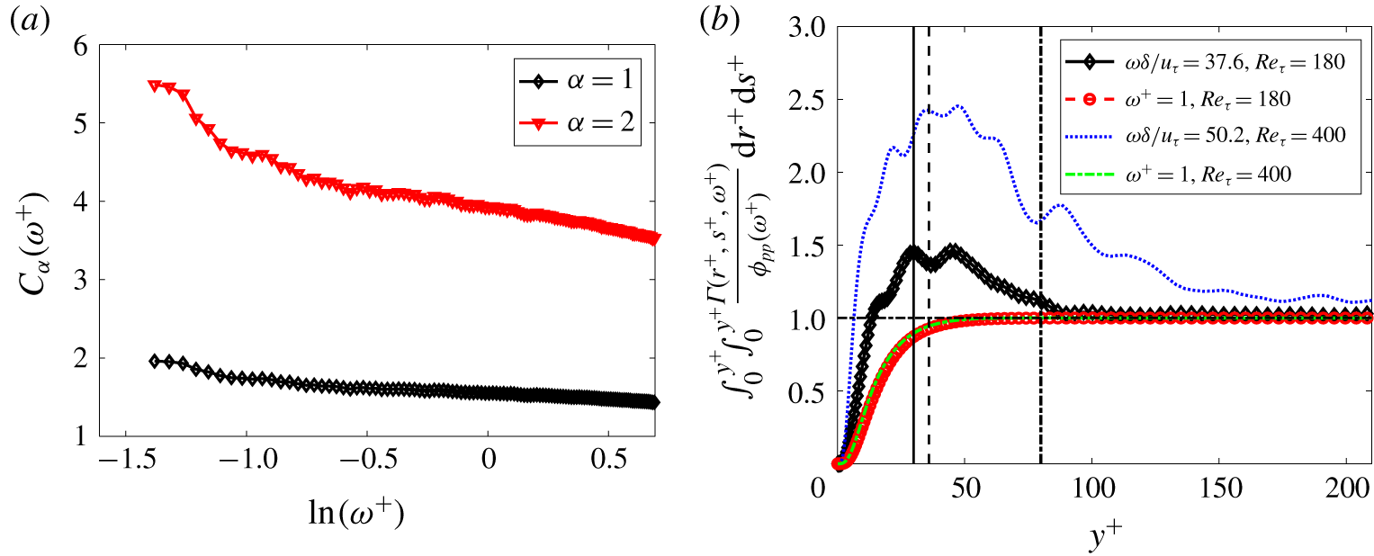
The variation of $C_{\unicode[STIX]{x1D6FC}}(\unicode[STIX]{x1D714}^{+})$ for $\unicode[STIX]{x1D6FC}=1,2$ using $Re_{\unicode[STIX]{x1D70F}}=400$ data is shown in figure 9(a). The proportionality constant is observed to vary slowly for $\unicode[STIX]{x1D714}^{+}>\ln (-1)$. Hence, in this frequency range, the width of the dominant net source is proportional to its location.

Figure 9.

(a) Variation of $C_{\unicode[STIX]{x1D6FC}}(\unicode[STIX]{x1D714}^{+})$ for $Re_{\unicode[STIX]{x1D70F}}=400$. (b) Partial wall-pressure fluctuation spectra from sources that extend from the wall to a particular $y^{+}$ for $Re_{\unicode[STIX]{x1D70F}}=180$ and 400 in near-wall region. The vertical solid, dashed, dash-dotted lines denote $y^{+}=30$, $y/\unicode[STIX]{x1D6FF}=0.2$ for $Re_{\unicode[STIX]{x1D70F}}=180$ and $y/\unicode[STIX]{x1D6FF}=0.2$ for $Re_{\unicode[STIX]{x1D70F}}=400$, respectively. The horizontal dash-dotted line denotes partial contribution equal to 1.

The contribution of the interaction between the net sources in the inner and overlap/outer region to wall-pressure PSD can be investigated using the wall-pressure fluctuation – net source CSD. Figure 9(b) shows the partial contribution (normalized by the wall-pressure PSD) $\int _{0}^{y^{+}}\int _{0}^{y^{+}}\unicode[STIX]{x1D6E4}(r^{+},s^{+},\unicode[STIX]{x1D714}^{+})/\unicode[STIX]{x1D719}_{pp}(\unicode[STIX]{x1D714}^{+})\text{d}r^{+}\text{d}s^{+}$ from the net sources contained between the wall and a given $y^{+}$ for two selected frequencies. At the low-frequency wall-pressure linear PSD peak (which is $\unicode[STIX]{x1D714}\unicode[STIX]{x1D6FF}/u_{\unicode[STIX]{x1D70F}}=37.6$ and $\unicode[STIX]{x1D714}\unicode[STIX]{x1D6FF}/u_{\unicode[STIX]{x1D70F}}=50.2$ for $Re_{\unicode[STIX]{x1D70F}}=180$ and 400, respectively), we observe that the partial contribution first increases and then decreases. However, a monotonically increasing behaviour is observed for the high frequency. In order to investigate the implication of the non-monotonic low-frequency behaviour, we split the domain $0<y/\unicode[STIX]{x1D6FF}<1$ into an inner region $0<y^{+}<30$, an outer/overlap region $30<y^{+}<Re_{\unicode[STIX]{x1D70F}}$. The contribution to wall-pressure PSD from sources within $y/\unicode[STIX]{x1D6FF}=1$ can then be accordingly split as

(4.5)$$\begin{eqnarray}\displaystyle & & \displaystyle \int _{0}^{Re_{\unicode[STIX]{x1D70F}}}\int _{0}^{Re_{\unicode[STIX]{x1D70F}}}{\displaystyle \frac{\unicode[STIX]{x1D6E4}(r^{+},s^{+},\unicode[STIX]{x1D714}^{+})}{\unicode[STIX]{x1D719}_{pp}(\unicode[STIX]{x1D714}^{+})}}\,\text{d}r^{+}\,\text{d}s^{+}\nonumber\\ \displaystyle & & \displaystyle \quad =\int _{0}^{30}\int _{0}^{30}{\displaystyle \frac{\unicode[STIX]{x1D6E4}(r^{+},s^{+},\unicode[STIX]{x1D714}^{+})}{\unicode[STIX]{x1D719}_{pp}(\unicode[STIX]{x1D714}^{+})}}\,\text{d}r^{+}\,\text{d}s^{+}+\int _{30}^{Re_{\unicode[STIX]{x1D70F}}}\int _{30}^{Re_{\unicode[STIX]{x1D70F}}}{\displaystyle \frac{\unicode[STIX]{x1D6E4}(r^{+},s^{+},\unicode[STIX]{x1D714}^{+})}{\unicode[STIX]{x1D719}_{pp}(\unicode[STIX]{x1D714}^{+})}}\,\text{d}r^{+}\,\text{d}s^{+}\nonumber\\ \displaystyle & & \displaystyle \qquad +\,2Re\left(\int _{0}^{30}\int _{30}^{Re_{\unicode[STIX]{x1D70F}}}{\displaystyle \frac{\unicode[STIX]{x1D6E4}(r^{+},s^{+},\unicode[STIX]{x1D714}^{+})}{\unicode[STIX]{x1D719}_{pp}(\unicode[STIX]{x1D714}^{+})}}\,\text{d}r^{+}\,\text{d}s^{+}\right).\end{eqnarray}$$

From figure 9(b), we observe that at the lower frequency, this contribution from sources within $y/\unicode[STIX]{x1D6FF}=1$ is smaller than the inner region contribution $\int _{0}^{30}\int _{0}^{30}(\unicode[STIX]{x1D6E4}(r^{+},s^{+},\unicode[STIX]{x1D714}^{+})/\unicode[STIX]{x1D719}_{pp}(\unicode[STIX]{x1D714}^{+}))\,\text{d}r^{+}\,\text{d}s^{+}$. Therefore,

(4.6)$$\begin{eqnarray}\int _{30}^{Re_{\unicode[STIX]{x1D70F}}}\int _{30}^{Re_{\unicode[STIX]{x1D70F}}}{\displaystyle \frac{\unicode[STIX]{x1D6E4}(r^{+},s^{+},\unicode[STIX]{x1D714}^{+})}{\unicode[STIX]{x1D719}_{pp}(\unicode[STIX]{x1D714}^{+})}}\,\text{d}r^{+}\,\text{d}s^{+}\leqslant -2Re\left(\int _{0}^{30}\int _{30}^{Re_{\unicode[STIX]{x1D70F}}}{\displaystyle \frac{\unicode[STIX]{x1D6E4}^{+}(r^{+},s^{+},\unicode[STIX]{x1D714}^{+})}{\unicode[STIX]{x1D719}_{pp}(\unicode[STIX]{x1D714}^{+})}}\,\text{d}r^{+}\,\text{d}s^{+}\right).\end{eqnarray}$$

Note the left-hand side of the above inequality is a positive real number. This indicates that (i) the contribution from the cross-correlations between the inner and the overlap/outer region dominates the contribution from the outer/overlap region alone, (ii) the phase difference between the net sources in these two regions is predominantly in the range $\unicode[STIX]{x03C0}/2$ to $\unicode[STIX]{x03C0}$ or $-\unicode[STIX]{x03C0}$ to $-\unicode[STIX]{x03C0}/2$. In other words, a positive (or negative) low-frequency event in the near-wall region is predominantly correlated with a negative (or positive) low-frequency event in the overlap/outer region. Therefore, the observed non-monotonic behaviour at low frequencies implies a dominant interaction between the net sources in the inner and outer regions of the channel at such frequencies. Such inner–outer interaction at long streamwise wavelengths has been previously observed for the streamwise velocity fluctuations by Del Álamo & Jiménez (Reference Del Álamo and Jiménez2003) and Morrison (Reference Morrison2007), and is the reason for the mixed scaling (De Graaff & Eaton Reference De Graaff and Eaton2000) of the streamwise velocity r.m.s. peak in wall-bounded flows.

We further investigate the fractional contributions of the wall-pressure sources in the inner ($y^{+}<30$), overlap ($30<y^{+}<0.2Re_{\unicode[STIX]{x1D70F}}$) and outer regions ($0.2<y/\unicode[STIX]{x1D6FF}<1$) and their cross-correlations to the wall-pressure PSD by splitting $\int _{0}^{Re_{\unicode[STIX]{x1D70F}}}\int _{0}^{Re_{\unicode[STIX]{x1D70F}}}(\unicode[STIX]{x1D6E4}(r^{+},s^{+},\unicode[STIX]{x1D714}^{+})/\unicode[STIX]{x1D719}_{pp}(\unicode[STIX]{x1D714}^{+}))\,\text{d}r^{+}\,\text{d}s^{+}$ into the sum,

(4.7)$$\begin{eqnarray}\displaystyle & & \displaystyle \int _{0}^{Re_{\unicode[STIX]{x1D70F}}}\int _{0}^{Re_{\unicode[STIX]{x1D70F}}}{\displaystyle \frac{\unicode[STIX]{x1D6E4}(r^{+},s^{+},\unicode[STIX]{x1D714}^{+})}{\unicode[STIX]{x1D719}_{pp}(\unicode[STIX]{x1D714}^{+})}}\,\text{d}r^{+}\,\text{d}s^{+}=\underbrace{\int _{0}^{30}\int _{0}^{30}{\displaystyle \frac{\unicode[STIX]{x1D6E4}(r^{+},s^{+},\unicode[STIX]{x1D714}^{+})}{\unicode[STIX]{x1D719}_{pp}(\unicode[STIX]{x1D714}^{+})}}\,\text{d}r^{+}\,\text{d}s^{+}}_{C_{11}}\nonumber\\ \displaystyle & & \displaystyle \quad +\,\underbrace{\int _{30}^{0.2Re_{\unicode[STIX]{x1D70F}}}\int _{30}^{0.2Re_{\unicode[STIX]{x1D70F}}}{\displaystyle \frac{\unicode[STIX]{x1D6E4}(r^{+},s^{+},\unicode[STIX]{x1D714}^{+})}{\unicode[STIX]{x1D719}_{pp}(\unicode[STIX]{x1D714}^{+})}}\,\text{d}r^{+}\,\text{d}s^{+}}_{C_{22}}+\underbrace{\int _{0.2Re_{\unicode[STIX]{x1D70F}}}^{Re_{\unicode[STIX]{x1D70F}}}\int _{0.2Re_{\unicode[STIX]{x1D70F}}}^{Re_{\unicode[STIX]{x1D70F}}}{\displaystyle \frac{\unicode[STIX]{x1D6E4}(r^{+},s^{+},\unicode[STIX]{x1D714}^{+})}{\unicode[STIX]{x1D719}_{pp}(\unicode[STIX]{x1D714}^{+})}}\,\text{d}r^{+}\,\text{d}s^{+}}_{C_{33}}\nonumber\\ \displaystyle & & \displaystyle \quad +\,2Re\!\left(\underbrace{\int _{0}^{30}\int _{30}^{0.2Re_{\unicode[STIX]{x1D70F}}}{\displaystyle \frac{\unicode[STIX]{x1D6E4}(r^{+},s^{+},\unicode[STIX]{x1D714}^{+})}{\unicode[STIX]{x1D719}_{pp}(\unicode[STIX]{x1D714}^{+})}}\,\text{d}r^{+}\,\text{d}s^{+}}_{C_{12}}+\underbrace{\int _{30}^{0.2Re_{\unicode[STIX]{x1D70F}}}\int _{0.2Re_{\unicode[STIX]{x1D70F}}}^{Re_{\unicode[STIX]{x1D70F}}}{\displaystyle \frac{\unicode[STIX]{x1D6E4}(r^{+},s^{+},\unicode[STIX]{x1D714}^{+})}{\unicode[STIX]{x1D719}_{pp}(\unicode[STIX]{x1D714}^{+})}}\,\text{d}r^{+}\,\text{d}s^{+}}_{C_{23}}\right.\nonumber\\ \displaystyle & & \displaystyle \quad +\left.\underbrace{\int _{0.2Re_{\unicode[STIX]{x1D70F}}}^{Re_{\unicode[STIX]{x1D70F}}}\int _{0}^{30}{\displaystyle \frac{\unicode[STIX]{x1D6E4}(r^{+},s^{+},\unicode[STIX]{x1D714}^{+})}{\unicode[STIX]{x1D719}_{pp}(\unicode[STIX]{x1D714}^{+})}}\,\text{d}r^{+}\,\text{d}s^{+}}_{C_{31}}\right)\!.\end{eqnarray}$$

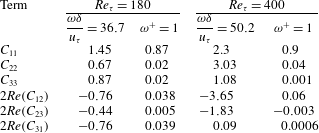
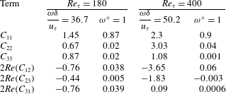
Table 2 shows the value of each term on the right-hand side of the above equation at the two $Re_{\unicode[STIX]{x1D70F}}$ for the same frequencies chosen in figure 9(b). For the lower frequency, we observe that the magnitude of the contribution from the cross-correlations between the regions is comparable to the contribution within the regions. However, at high frequency, the contribution within each region dominates over the cross-correlation between the regions. The real part of the cross-correlations is negative at the lower frequency for $Re_{\unicode[STIX]{x1D70F}}=180$. As discussed in the previous paragraph, this implies that the phase difference of the wall-pressure sources in the different regions lie in the range $\unicode[STIX]{x03C0}/2$ to $\unicode[STIX]{x03C0}$ or $-\unicode[STIX]{x03C0}/2$ to $-\unicode[STIX]{x03C0}$. For the higher $Re_{\unicode[STIX]{x1D70F}}$, except the inner and outer regions $(2Re(C_{31}))$, the phase difference between all the other regions lies in the same range as the lower $Re_{\unicode[STIX]{x1D70F}}$. Overall, we observe that the cross-correlations between the wall-pressure sources present in the inner, overlap and outer regions are important contributors to the PSD at low frequency but not at high frequency.

Further, this framework can be used to identify the location of the dominant sources that lead to the $\unicode[STIX]{x1D714}^{-1}$ behaviour of the wall-pressure PSD in the mid-frequency range (observed at very high Reynolds numbers). Farabee & Casarella (Reference Farabee and Casarella1991) noted that the $\unicode[STIX]{x1D714}^{-1}$ behaviour is responsible for the logarithmic dependence of the wall-pressure r.m.s. on Reynolds number (Abe et al. Reference Abe, Matsuo and Kawamura2005; Hu et al. Reference Hu, Morfey and Sandham2006; Jimenez & Hoyas Reference Jimenez and Hoyas2008).

Table 2.

Fractional contributions of the inner, overlap and outer regions to the wall-pressure fluctuation PSD. For definitions of $C_{11}$, $C_{22}$, $C_{33}$, $C_{12}$, $C_{23}$ and $C_{31}$, see (4.7).

4.3 Spectral POD of net source CSD

Before we investigate the spectral POD modes of the net source CSD, we first examine the relevance of the modes to wall-pressure fluctuation. We can decompose the wall-pressure fluctuation $p(x,0,z,t)$ at a typical point $(x,z)$ on the wall by expressing its Fourier transform $\hat{p}(x,0,z,\unicode[STIX]{x1D714})$ (equation (3.5)) in terms of the spectral POD modes. We have

(4.8)$$\begin{eqnarray}\displaystyle & \displaystyle p(x,0,z,t)=\int _{-\infty }^{+\infty }\hat{p}(x,0,z,\unicode[STIX]{x1D714})\text{e}^{\text{i}\unicode[STIX]{x1D714}t}\,\text{d}\unicode[STIX]{x1D714}, & \displaystyle\end{eqnarray}$$

(4.9)$$\begin{eqnarray}\displaystyle & \displaystyle p(x,0,z,t)=\int _{-\infty }^{+\infty }\left(\int _{-\unicode[STIX]{x1D6FF}}^{+\unicode[STIX]{x1D6FF}}\hat{f}_{G}(x,y,z,\unicode[STIX]{x1D714})\,\text{d}y\right)\text{e}^{\text{i}\unicode[STIX]{x1D714}t}\,\text{d}\unicode[STIX]{x1D714}. & \displaystyle\end{eqnarray}$$

We use the decomposition in (3.18) to express $\hat{f}_{G}(x,y,z,\unicode[STIX]{x1D714})$ in terms of the spectral POD modes and obtain

(4.10)$$\begin{eqnarray}p(x,0,z,t)=\int _{-\infty }^{+\infty }\mathop{\sum }_{j=1}^{\infty }\unicode[STIX]{x1D6FC}_{i}(x,z,\unicode[STIX]{x1D714})\left(\int _{-\unicode[STIX]{x1D6FF}}^{+\unicode[STIX]{x1D6FF}}\unicode[STIX]{x1D6F7}_{j}^{\ast }(y,\unicode[STIX]{x1D714})\,\text{d}y\right)\text{e}^{\text{i}\unicode[STIX]{x1D714}t}\,\text{d}\unicode[STIX]{x1D714}.\end{eqnarray}$$

Rearranging the integral and writing $\unicode[STIX]{x1D6F7}_{j}(y,\unicode[STIX]{x1D714})$ as $|\unicode[STIX]{x1D6F7}_{j}(y,\unicode[STIX]{x1D714})|\text{e}^{-\text{i}\angle \unicode[STIX]{x1D6F7}_{j}(y,\unicode[STIX]{x1D714})}$, we obtain

(4.11)$$\begin{eqnarray}p(x,0,z,t)=\int _{-\unicode[STIX]{x1D6FF}}^{+\unicode[STIX]{x1D6FF}}\int _{-\infty }^{+\infty }\mathop{\sum }_{j=1}^{\infty }\unicode[STIX]{x1D6FC}_{j}(x,z,\unicode[STIX]{x1D714})|\unicode[STIX]{x1D6F7}_{j}(y,\unicode[STIX]{x1D714})|\text{e}^{\text{i}(-\angle \unicode[STIX]{x1D6F7}_{j}(y,\unicode[STIX]{x1D714})+\unicode[STIX]{x1D714}t)}\,\text{d}\unicode[STIX]{x1D714}\,\text{d}y.\end{eqnarray}$$

The above equation expresses the wall-pressure fluctuation as a contribution from each spectral POD mode. Recall that the individual contributions are decorrelated, i.e. $\langle \unicode[STIX]{x1D6FC}_{i}(x,z,\unicode[STIX]{x1D714})\unicode[STIX]{x1D6FC}_{j}^{\ast }(x,z,\unicode[STIX]{x1D714}_{o})\rangle =\unicode[STIX]{x1D706}_{i}(\unicode[STIX]{x1D714})\unicode[STIX]{x1D6FF}_{ij}\unicode[STIX]{x1D6FF}(\unicode[STIX]{x1D714}-\unicode[STIX]{x1D714}_{o})$, where $\unicode[STIX]{x1D6FF}$ is the Dirac delta function. Note that, since we integrate over all wavenumbers, the contribution of coherent structures of all length scales is included.

The wall-normal phase velocity of the net sources represented by the $i\text{th}$ spectral POD mode can be quantified as a function of the wall-normal distance using the phase $\angle \unicode[STIX]{x1D6F7}_{i}(y,\unicode[STIX]{x1D714})$. We define a local wall-normal phase velocity $c_{i}^{+}(y^{+},\unicode[STIX]{x1D714}^{+})$ in viscous units as

(4.12)$$\begin{eqnarray}c_{i}^{+}(y^{+},\unicode[STIX]{x1D714}^{+})=\unicode[STIX]{x1D714}^{+}/k_{i}^{+}(y^{+},\unicode[STIX]{x1D714}^{+}),\end{eqnarray}$$

where the local wavenumber $k_{i}^{+}(y^{+},\unicode[STIX]{x1D714}^{+})$ is defined as $k_{i}^{+}(y^{+},\unicode[STIX]{x1D714}^{+})=\unicode[STIX]{x2202}\angle \unicode[STIX]{x1D6F7}_{i}(y^{+},\unicode[STIX]{x1D714}^{+})/\unicode[STIX]{x2202}y^{+}$. Note that a negative phase velocity indicates an enclosed wave travelling towards the wall and vice versa. Also, this is similar to estimating the instantaneous frequency of a temporal signal using Hilbert transform (Huang & Shen Reference Huang and Shen2014).

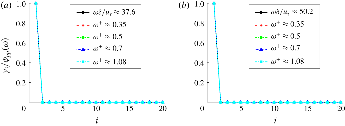
We found that, for a wide range of frequencies, setting $\unicode[STIX]{x1D6FD}$ (3.16) to 0.1 gives a dominant spectral POD mode ($\unicode[STIX]{x1D6F7}_{1}$) that contributes to all of the wall-pressure PSD (see figure 10). This observation is consistent with the discussion after (3.20). Note that the lowest frequency in figure 10 corresponds to the low-frequency peak in the linear PSD. Also, $\unicode[STIX]{x1D714}^{+}=0.35$ is the location of the premultiplied PSD peak. Therefore, the dominant modes at these peak frequencies represent the decorrelated source responsible for the peaks.

Further, the dominant mode represents the active part of the net source Fourier transform ($\hat{f}_{G}(x,y,z,\unicode[STIX]{x1D714})$). It is active in the sense that it contributes to the entire PSD. The remaining portion of $\hat{f}_{G}(x,y,z,\unicode[STIX]{x1D714})$ is inactive in the sense that it does not contribute to the wall-pressure PSD. The suboptimal spectral POD modes comprise this inactive portion. Essentially, the contribution of the suboptimal modes from different wall-normal locations undergo destructive interference resulting in zero net contribution. Since the active and inactive parts of $\hat{f}_{G}(x,y,z,\unicode[STIX]{x1D714})$ stem from different modes, they are decorrelated.

Separating the active and inactive parts of $\hat{f}_{G}(x,y,z,\unicode[STIX]{x1D714})$ in (3.18), we have

(4.13)$$\begin{eqnarray}\left.\begin{array}{@{}c@{}}\hat{f}_{g}(x,y,z,\unicode[STIX]{x1D714})=\unicode[STIX]{x1D6FC}_{1}(x,z,\unicode[STIX]{x1D714})\unicode[STIX]{x1D6F7}_{1}^{\ast }(y,\unicode[STIX]{x1D714})+I(x,y,z,\unicode[STIX]{x1D714}),\\ I(x,y,z,\unicode[STIX]{x1D714})=\displaystyle \mathop{\sum }_{j=2}^{\infty }\unicode[STIX]{x1D6FC}_{j}(x,z,\unicode[STIX]{x1D714})\unicode[STIX]{x1D6F7}_{j}^{\ast }(y,\unicode[STIX]{x1D714}),\end{array}\right\}\end{eqnarray}$$

where $\unicode[STIX]{x1D6FC}_{1}(x,z,\unicode[STIX]{x1D714})\unicode[STIX]{x1D6F7}_{1}^{\ast }(y,\unicode[STIX]{x1D714})$ and $I(x,y,z,\unicode[STIX]{x1D714})$ are the active and inactive portions of $\hat{f}_{G}(x,y,z,\unicode[STIX]{x1D714})$, respectively. Correlating the two, we obtain

(4.14)$$\begin{eqnarray}\displaystyle \langle \unicode[STIX]{x1D6FC}_{1}^{\ast }(x,z,\unicode[STIX]{x1D714})\unicode[STIX]{x1D6F7}_{1}(r,\unicode[STIX]{x1D714})I(x,s,z,\unicode[STIX]{x1D714}_{o})\rangle & = & \displaystyle \mathop{\sum }_{j=2}^{\infty }\langle \unicode[STIX]{x1D6FC}_{1}^{\ast }(x,z,\unicode[STIX]{x1D714})\unicode[STIX]{x1D6FC}_{j}(x,z,\unicode[STIX]{x1D714})\rangle \unicode[STIX]{x1D6F7}_{1}(r,\unicode[STIX]{x1D714})\unicode[STIX]{x1D6F7}_{j}^{\ast }(s,\unicode[STIX]{x1D714}_{o})\nonumber\\ \displaystyle & = & \displaystyle \mathop{\sum }_{j=2}^{\infty }\unicode[STIX]{x1D706}_{1}\unicode[STIX]{x1D6FF}_{j1}\unicode[STIX]{x1D6F7}_{1}(r,\unicode[STIX]{x1D714})\unicode[STIX]{x1D6F7}_{j}^{\ast }(s,\unicode[STIX]{x1D714}_{o})\;(\text{using }(3.18))\nonumber\\ \displaystyle & = & \displaystyle 0.\end{eqnarray}$$

Therefore, both parts are decorrelated. Note that $I(x,y,z,\unicode[STIX]{x1D714})$, the inactive part, is orthogonal to the eigenfunction $\bar{\unicode[STIX]{x1D6F7}}_{1}^{\ast }(y,\unicode[STIX]{x1D714})$ (equation (3.15)) in the $L^{2}$ inner product. Decreasing $\unicode[STIX]{x1D6FD}$ to even smaller values does not affect the mode shape or the eigenvalues for the frequencies in figure 10.

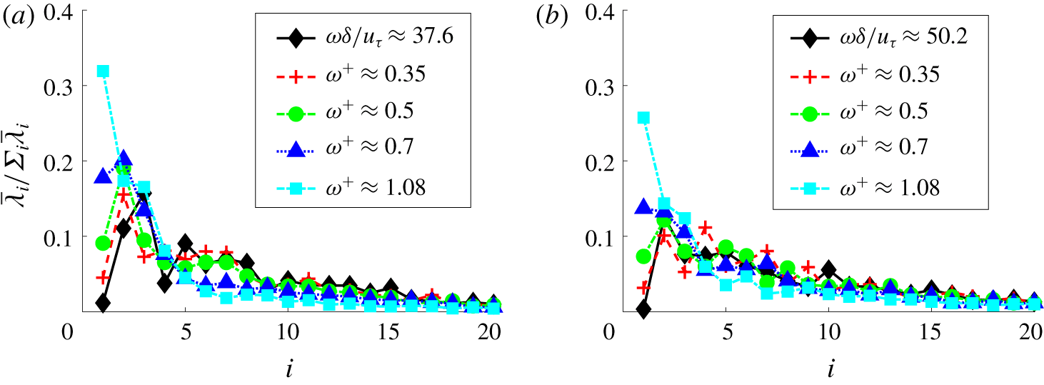
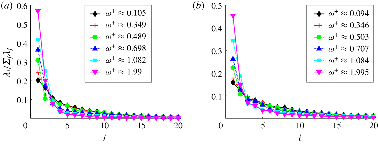
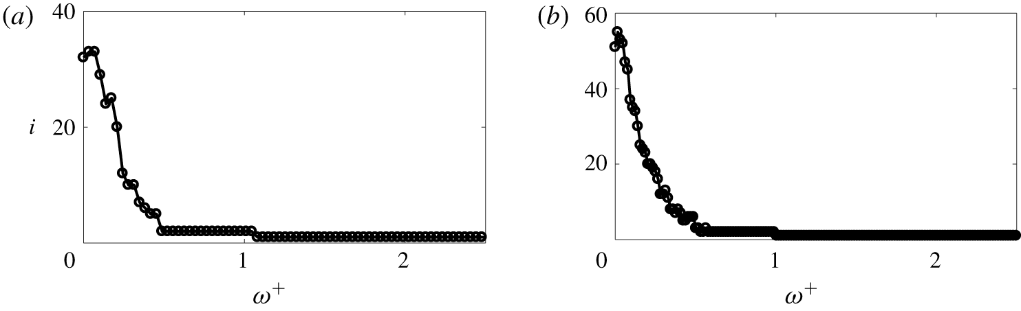
Since we use a Poisson inner product, the dominant spectral POD mode need not be energetically dominant. In other words, it need not contribute the most to the integrated net source PSD ($\int _{-\unicode[STIX]{x1D6FF}}^{+\unicode[STIX]{x1D6FF}}\unicode[STIX]{x1D6E4}(r,r,\unicode[STIX]{x1D714})\,\text{d}r$). Figure 11 shows this behaviour for low frequencies. In the figure, $\bar{\unicode[STIX]{x1D706}}_{j}(\unicode[STIX]{x1D714})=\unicode[STIX]{x1D706}_{j}(\unicode[STIX]{x1D714})|\int _{-\unicode[STIX]{x1D6FF}}^{+\unicode[STIX]{x1D6FF}}\unicode[STIX]{x1D6F7}_{j}(y,\unicode[STIX]{x1D714})\,\text{d}y|^{2}$ is the contribution of the $j$th mode to the integrated PSD. We observe that the fractional contribution of the dominant mode increases with frequency. At $\unicode[STIX]{x1D714}^{+}=1$, the dominant spectral POD mode is the energetically dominant mode.

Figure 10.

Fractional contribution of the first 20 spectral POD modes computed using the Poisson inner product ($\unicode[STIX]{x1D6FD}=0.1$) to the wall-pressure PSD for (a) $Re_{\unicode[STIX]{x1D70F}}=180$ and (b) $Re_{\unicode[STIX]{x1D70F}}=400$ at different frequencies.

Figure 11.

Fractional contribution of the first 20 spectral POD modes computed using the Poisson inner product ($\unicode[STIX]{x1D6FD}=0.1$) to the integrated net source PSD for (a) $Re_{\unicode[STIX]{x1D70F}}=180$ and (b) $Re_{\unicode[STIX]{x1D70F}}=400$ at different frequencies.

Figure 12.

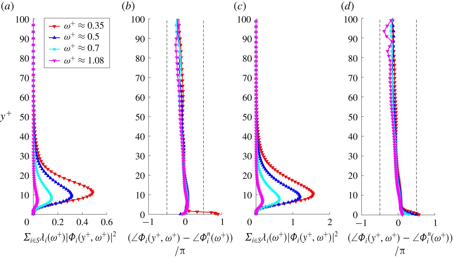
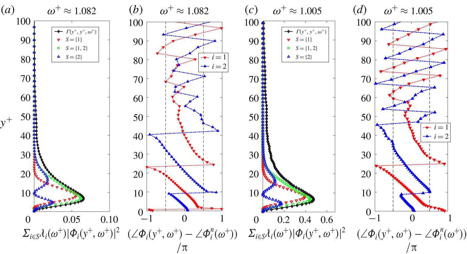
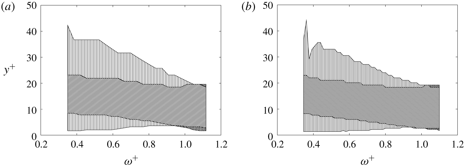
Envelope (a,c) and phase (b,d) of the dominant spectral POD mode computed using the Poisson inner product ($\unicode[STIX]{x1D6FD}=0.1$) for a few selected high frequencies. Panels (a,b) and (c,d) are for $Re_{\unicode[STIX]{x1D70F}}=180$ and 400, respectively. The left and right dashed black solid line in (b,d) indicate $\angle \unicode[STIX]{x1D6F7}_{i}(y^{+},\unicode[STIX]{x1D714}^{+})-\angle \unicode[STIX]{x1D6F7}_{i}^{n}(\unicode[STIX]{x1D714}^{+})$ equal to $-\unicode[STIX]{x03C0}/2$ and $\unicode[STIX]{x03C0}/2$, respectively.

Figure 12 shows the wall-normal variation of the envelope and phase of the dominant mode at the premultiplied spectrum peak $\unicode[STIX]{x1D714}^{+}=0.35$ and a few higher frequencies $\unicode[STIX]{x1D714}^{+}=0.5$, 0.7 and 1. The dominant modes have a similar shape in inner units for both $Re_{\unicode[STIX]{x1D70F}}$. Its envelope (figure 12a,c) represents sources confined near the wall with intensities peaking in the buffer layer. With increasing frequency, the wall-normal location of the peak moves closer to the wall, and the width of the envelope decreases. This behaviour of the dominant mode is consistent with that of the wall-pressure fluctuation – net source CSD. The phase (figure 12b,d) of the dominant mode varies between $-\unicode[STIX]{x03C0}/2$ and $\unicode[STIX]{x03C0}/2$. Therefore, the contributions from different wall-normal locations undergo constructive interference. Further, the phase variation is almost linear with a negative slope, at least around the envelope peak. The negative slope indicates that the envelope encloses a wave travelling towards the wall.

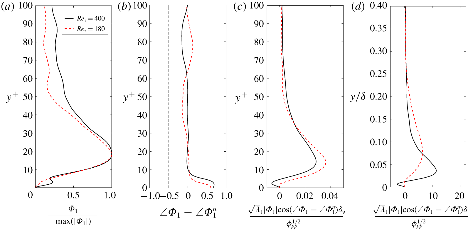
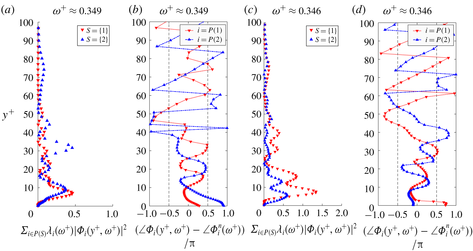
Figures 13(a) and 13(b) show the magnitude and phase, respectively, of the dominant spectral POD mode at the low-frequency linear PSD peak (figure 4). Recall that the frequencies are $\unicode[STIX]{x1D714}\unicode[STIX]{x1D6FF}/u_{\unicode[STIX]{x1D70F}}=37.6$ for $Re_{\unicode[STIX]{x1D70F}}=180$ and 50.2 for $Re_{\unicode[STIX]{x1D70F}}=400$. The envelope of the dominant mode peaks around $y^{+}\approx 15$ for both $Re_{\unicode[STIX]{x1D70F}}$. The phase variation does not show any noticeable slope indicating that the different wall-normal locations are in phase with each other, at least around the envelope peak.

In figures 13(c) and 13(d), we show the wall-normal contribution of the dominant mode to the wall-pressure PSD in inner and outer units, respectively. The curves are normalized to obtain unit integral along the $y$-axis. The contribution peaks at $y^{+}\approx 15$ for both $Re_{\unicode[STIX]{x1D70F}}$. Also, figure 13(c) shows a negative contribution close to the wall for $Re_{\unicode[STIX]{x1D70F}}=400$ that is not present for $Re_{\unicode[STIX]{x1D70F}}=180$. We observe that the region $y^{+}>30$ contributes more for the higher Reynolds number, signifying an increase in the outer region contribution. Further, from figure 13(d), we observe that the width of this dominant source is around $0.25\unicode[STIX]{x1D6FF}$ since the $y$-coordinate is significant for $y<0.25\unicode[STIX]{x1D6FF}$. Overall, at the low-frequency PSD peak, the contribution from the dominant mode peaks at $y^{+}=15$, and its width is around $0.25\unicode[STIX]{x1D6FF}$.

Figure 13.

Envelope (a) and phase (b) of the dominant spectral POD mode computed using the Poisson inner product at the low-frequency linear PSD peak. Panels (c,d) show the normalized wall-normal contribution of the dominant mode to the wall-pressure PSD in inner and outer units, respectively.

Figure 14.

Representative net source $\tilde{f}_{G}$ at the premultiplied spectrum peak (a,b) and the linear spectrum peak (c,d). Panels (a,c) are for $Re_{\unicode[STIX]{x1D70F}}=180$, and (b,d) are for $Re_{\unicode[STIX]{x1D70F}}=400$. Contours in (a,b) are 10 equally spaced values between the minimum and maximum of $\tilde{f}_{G}$. Contours in (c,d) are $[\pm 0.05\,\pm 0.1\,\pm 0.2\,\pm 0.5\,\pm 0.8]$ times the maximum value of $\tilde{f}_{G}$.

We create a representative net source field that gives the two-dimensional structure implied by a spectral POD mode. The representative field $\tilde{f}_{G}(x,y,z,t)$ implied by mode $\unicode[STIX]{x1D6F7}_{j}(y,\unicode[STIX]{x1D714}_{o})$ at frequency $\unicode[STIX]{x1D714}_{o}$ is constructed as

(4.15)$$\begin{eqnarray}\tilde{f}_{G}(x,y,z,t)=Re(\unicode[STIX]{x1D6FC}(x,z,\unicode[STIX]{x1D714}_{o})\text{e}^{-\text{i}\angle \unicode[STIX]{x1D6F7}_{j}(y,\unicode[STIX]{x1D714}_{o})}|\unicode[STIX]{x1D6F7}_{j}(y,\unicode[STIX]{x1D714}_{o})|\text{e}^{\text{i}\unicode[STIX]{x1D714}_{o}t}),\end{eqnarray}$$

where $Re(f)$ is the real part of $f$. Since $\unicode[STIX]{x1D6FC}(x,z,\unicode[STIX]{x1D714}_{o})$ is homogeneous in $x$ and $z$, we decompose it using the Fourier transform. Intuitively, we expect the streamwise convective Fourier component $\text{e}^{-\text{i}\unicode[STIX]{x1D714}_{o}x/c_{o}(\unicode[STIX]{x1D714}_{o})}$ of $\unicode[STIX]{x1D6FC}(x,z,\unicode[STIX]{x1D714}_{o})$ to be the most dominant one. Here, $c_{o}(\unicode[STIX]{x1D714}_{o})$ is the convective velocity at frequency $\unicode[STIX]{x1D714}_{o}$. For simplicity, we assume no spanwise variation of the representative net source. Substituting $\unicode[STIX]{x1D6FC}(x,z,\unicode[STIX]{x1D714}_{o})=\text{e}^{-\text{i}\unicode[STIX]{x1D714}_{o}x/c_{o}(\unicode[STIX]{x1D714}_{o})}$ in the above equation, we obtain the representative field

(4.16)$$\begin{eqnarray}\tilde{f}_{G}(x,y,z,t)=Re(\text{e}^{-\text{i}\unicode[STIX]{x1D714}_{o}x/c_{o}(\unicode[STIX]{x1D714}_{o})}\text{e}^{-\text{i}\angle \unicode[STIX]{x1D6F7}_{j}(y,\unicode[STIX]{x1D714}_{o})}|\unicode[STIX]{x1D6F7}_{j}(y,\unicode[STIX]{x1D714}_{o})|\text{e}^{\text{i}\unicode[STIX]{x1D714}_{o}t}).\end{eqnarray}$$

To create the representative field at a frequency $\unicode[STIX]{x1D714}_{o}$, we need three inputs – the mode $\unicode[STIX]{x1D6F7}_{j}(y,\unicode[STIX]{x1D714}_{o})$, the convection velocity $c_{o}(\unicode[STIX]{x1D714}_{o})$ and the time $t$. Figure 14 shows the representative net source field constructed from the dominant spectral POD mode. Figures 14(a,b) are at the premultiplied PSD peak frequency and figures 14(c,d) are at the linear PSD peak frequency. We use a convection velocity defined as $c_{o}(\unicode[STIX]{x1D714}_{o})/u_{\unicode[STIX]{x1D70F}}=(\unicode[STIX]{x1D714}_{o}\unicode[STIX]{x1D6FF}/u_{\unicode[STIX]{x1D70F}})/k_{p}(\unicode[STIX]{x1D714}_{o})\unicode[STIX]{x1D6FF}$, where $k_{p}(\unicode[STIX]{x1D714}_{o})$ is the peak wavenumber coordinate at frequency $\unicode[STIX]{x1D714}_{o}$ in the wavenumber–frequency spectrum of wall-pressure. We choose time $t$ to be 0.

Figure 14(a,b) shows a convecting coherent structure inclined in the downstream direction. Essentially, this is because of the negative slope in the phase of the mode. As the inclined structures convect across a fixed streamwise location $x_{o}^{+}$, the wall-normal intensity (magnitude of the field that depends on $y$ and $x_{o}$) propagates towards the wall as indicated by the negative slope.

Figure 14(c,d) shows the coherent structure represented by the dominant POD mode at the linear PSD peak. These structures are vertical, with almost no inclination in the downstream direction, as indicated by almost no slope in the phase of the mode. Such large scale vertical patterns with streamwise spacing of ${\sim}2\unicode[STIX]{x1D6FF}$ have been previously observed in the instantaneous rapid pressure fields for $Re_{\unicode[STIX]{x1D70F}}\sim 1000$ by Abe et al. (Reference Abe, Matsuo and Kawamura2005). They proposed that these patterns are responsible for the low-wavenumber peak in the wall-pressure spectra. The coherent structures in figure 14(c,d) further support this case.

Overall, the dominant spectral POD mode represents the active portion of the net source that contributes to the entire wall-pressure PSD. The remaining POD modes that comprise the inactive portion make zero contribution to the PSD. Further, the active and inactive parts are decorrelated. At high frequencies ($\unicode[STIX]{x1D714}^{+}\geqslant 0.35$), the shape of the dominant POD mode is similar in inner units for the two $Re_{\unicode[STIX]{x1D70F}}$. The two-dimensional (2-D) coherent structure at the premultiplied PSD peak inclines in the downstream direction. At the low-frequency linear PSD peak, the wall-normal contribution peaks in the buffer layer at $y^{+}\approx 15$ with a width of $y/\unicode[STIX]{x1D6FF}\approx 0.25$. The corresponding 2-D structure has a large scale vertical pattern similar to the previous observations of the instantaneous rapid pressure field by Abe et al. (Reference Abe, Matsuo and Kawamura2005).

We expect the similarity of the high-frequency dominant modes in inner units to continue at even higher Reynolds numbers. In the low wavenumber/frequency wall-pressure linear spectrum peak, the outer region $(y^{+}>30)$ contributes more for $Re_{\unicode[STIX]{x1D70F}}=400$ than for $Re_{\unicode[STIX]{x1D70F}}=180$. This low wavenumber/frequency peak is present in the linear wall-pressure spectra up to $Re_{\unicode[STIX]{x1D70F}}=5000$ (Abe et al. Reference Abe, Matsuo and Kawamura2005; Panton et al. Reference Panton, Lee and Moser2017). With increasing Reynolds number, we expect this contribution from the outer region to grow larger. Further, at $Re_{\unicode[STIX]{x1D70F}}\approx 5000$, the low- and high-wavenumber contributions to the premultiplied wall-pressure spectra show mild separation. We expect the spectral POD modes responsible for the low-wavenumber peak to depend on outer units. Further, high Reynolds number effects like amplitude modulation (Tsuji, Marusic & Johansson Reference Tsuji, Marusic and Johansson2016) in the wall-pressure sources could be studied using the above spectral POD framework.

Figure 15.

Spectral POD eigenvalues computed using the $L^{2}$ inner product for (a) $Re_{\unicode[STIX]{x1D70F}}=180$ and (b) $Re_{\unicode[STIX]{x1D70F}}=400$ at different frequencies.

Figure 16.

Contribution of the first 20 spectral POD modes computed using the $L^{2}$ inner product (normalized by the wall-pressure PSD) to wall-pressure PSD for (a) $Re_{\unicode[STIX]{x1D70F}}=180$ and (b) $Re_{\unicode[STIX]{x1D70F}}=400$ at different frequencies.

Figure 17.

Index of the spectral POD (computed using $L^{2}$ inner product) that contributes the most to the wall-pressure PSD for (a) $Re_{\unicode[STIX]{x1D70F}}=180$ and (b) $Re_{\unicode[STIX]{x1D70F}}=400$.

4.3.1 Remark on spectral POD with the $L^{2}$ inner product

We also performed spectral POD of the net source CSD using the $L^{2}$ inner product. Figure 15 shows the obtained eigenvalues for both $Re_{\unicode[STIX]{x1D70F}}$. The eigenvalues give the contribution of each POD mode to the wall-normal integral of the net source PSD. The POD modes obtained with the $L^{2}$ inner product, by definition, optimally decompose the integral of the net source PSD. However, the dominant POD mode might not contribute significantly to the wall-pressure PSD. Clearly, figure 16 shows this behaviour for $\unicode[STIX]{x1D714}^{+}<1$.

To investigate this further, we plot the index of the POD mode that contributes the most to the wall-pressure PSD as a function of frequency in figure 17. In the frequency ranges $0.55<\unicode[STIX]{x1D714}^{+}<1$ and $\unicode[STIX]{x1D714}^{+}>1$, the dominant wall-pressure mode (largest $\unicode[STIX]{x1D6FE}_{i}(\unicode[STIX]{x1D714})$) is the second and the first spectral POD mode, respectively. At low frequencies $\unicode[STIX]{x1D714}^{+}<0.55$, the dominant wall-pressure mode index is larger than or equal to 3. The dominant spectral POD mode is not the dominant wall-pressure mode because of destructive interference. The contributions of the dominant spectral POD mode from different wall-normal regions cancel each other out. For more details, we refer the reader to appendix D.

Figure 18.

Envelope (a,c) and phase (b,d) of the two dominant spectral POD modes computed using the $L^{2}$ inner product at different frequencies. Panels (a,b) and (c,d) are for $Re_{\unicode[STIX]{x1D70F}}=180$ and 400, respectively. The left and right dashed black solid lines in (b,d) indicate $\angle \unicode[STIX]{x1D6F7}_{i}(y^{+},\unicode[STIX]{x1D714}^{+})-\angle \unicode[STIX]{x1D6F7}_{i}^{n}(\unicode[STIX]{x1D714}^{+})$ equal to $-\unicode[STIX]{x03C0}/2$ and $\unicode[STIX]{x03C0}/2$, respectively.

The magnitude and phase of the first two dominant spectral POD modes at a high frequency of $\unicode[STIX]{x1D714}^{+}\approx 1$ are shown in figure 18. Note that, for this frequency, the dominant spectral POD and wall-pressure modes coincide. Clearly, we observe that the dominant modes resemble wavepackets. For both $Re_{\unicode[STIX]{x1D70F}}$, the envelope and phase of the wavepackets have a similar shape, which indicates similarity of the dominant modes at high frequencies. The envelope shows that dominant modes correspond to sources in the near-wall region ($y^{+}<30$). The first and second dominant mode envelopes have one and two lobes respectively (figure 18a,c). Since the slope of the phase variation of both modes is negative near the wall (figure 18b,d), equation (4.12) implies that these modes correspond to sources moving towards the wall.

Figure 19.

Envelope (a,c) and phase (b,d) of the two dominant wall-pressure modes computed using the $L^{2}$ inner product at $\unicode[STIX]{x1D714}^{+}=0.35$. Panels (a,b) and (c,d) are for $Re_{\unicode[STIX]{x1D70F}}=180$ and 400, respectively. The left and right dashed black solid lines in (b,d) indicate $\angle \unicode[STIX]{x1D6F7}_{i}(y^{+},\unicode[STIX]{x1D714}^{+})-\angle \unicode[STIX]{x1D6F7}_{i}^{n}(\unicode[STIX]{x1D714}^{+})$ equal to $-\unicode[STIX]{x03C0}/2$ and $\unicode[STIX]{x03C0}/2$, respectively. $P(S)$ is the spectral POD mode index of the $S$th dominant wall-pressure mode.

Next, we investigate the first two dominant wall-pressure modes at $\unicode[STIX]{x1D714}^{+}=0.35$, which together contribute approximately 50 % to the wall-pressure PSD in figure 19. Note that the premultiplied spectrum peak occurs at this frequency (figure 1b). The magnitude and phase variation shows that these modes do not resemble a near-wall wavepacket. The envelope is not localized and the phase variation shows no sign of linear variation. Not much can be said of the pattern of these low-frequency wall-pressure sources, except that the contributions from different wall-normal regions undergo constructive interference. This is because the phase of the mode varies mostly between the two dashed lines. Further, several suboptimal spectral POD modes each contribute a small fraction the wall-pressure PSD at this frequency (figure 16). Thus, the individual dominant wall-pressure mode obtained using the $L^{2}$ inner product does not give us much information of the wall-pressure sources. However, the mode obtained using the Poisson inner product with $\unicode[STIX]{x1D6FD}=0.1$ (figure 12) gives useful information of the wall-pressure source.

Therefore, spectral POD using the Poisson inner product performs better than the $L^{2}$ inner product in isolating dominant wall-pressure sources for both low and high frequencies. This is because the Poisson inner product decomposes the integral $\iint _{-\unicode[STIX]{x1D6FF}}^{+\unicode[STIX]{x1D6FF}}(G(s,r,(\unicode[STIX]{x1D6FD}/1-\unicode[STIX]{x1D6FD}),0)/1-\unicode[STIX]{x1D6FD})\unicode[STIX]{x1D6E4}(r,s,\unicode[STIX]{x1D714})\,\text{d}r\,\text{d}s$ as the sum of eigenvalues. For small enough $\unicode[STIX]{x1D6FD}$, this integral is a good proxy for wall-pressure PSD. On the other hand, the $L^{2}$ inner product decomposes the integrated net source PSD ($\int _{-\unicode[STIX]{x1D6FF}}^{+\unicode[STIX]{x1D6FF}}\unicode[STIX]{x1D6E4}(r,r,\unicode[STIX]{x1D714}),\text{d}r$) instead which is not a good proxy for the wall-pressure PSD.