Buoyancy-induced, columnar vortices

Mark W. Simpson; Ari Glezer

doi:10.1017/jfm.2016.541

Buoyancy-induced, columnar vortices

Published online by Cambridge University Press: 13 September 2016

Mark W. Simpson and

Ari Glezer

Show author details

Mark W. Simpson*: Affiliation:
George W. Woodruff School of Mechanical Engineering, Georgia Institute of Technology, Atlanta, GA 30332, USA
Ari Glezer: Affiliation:
George W. Woodruff School of Mechanical Engineering, Georgia Institute of Technology, Atlanta, GA 30332, USA
*: †Email address for correspondence: mws247@gmail.com

Article contents

Abstract
Introduction
Dimensional considerations
Experimental methodology
The structure of the columnar vortex
The near-surface vortex structure
Concluding remarks
References

Rights & Permissions

Abstract

A buoyancy-induced, columnar vortex is deliberately triggered in the unstably stratified air layer over a heated ground plane and is anchored within, and scales with, an azimuthal array of vertical, stator-like planar flow vanes that form an open-top enclosure and impart tangential momentum to the radially entrained air flow. The columnar vortex comprises three coupled primary flow domains: a spiraling surface momentum boundary layer of ground-heated air, an inner thermally driven vertical vortex core and an outer annular flow that is bounded by a helical shear layer and the vanes along its inner and outer edges, respectively, and by the spiraling boundary layer from below. In common with free buoyant columnar (dust devil) vortices that occur spontaneously over solar-heated terrain in the natural environment, the stationary anchored vortex is self-sustained by the conversion of the potential energy of the entrained surface-heated air layer to the kinetic energy of the induced vortical flow that persists as long as the thermal stratification is maintained. This conversion occurs as radial vorticity produced within the surface boundary layer is tilted vertically near the vortex centreline by the buoyant air to form the core of the columnar vortex. The structure and dynamics of the buoyant vortex are investigated using high-resolution stereo particle image velocimetry with specific emphasis on the evolution of the vorticity distributions and their effects on the characteristic scales of the ensuing vortex and on the kinetic energy of the induced flow.

JFM classification

Convection: Buoyancy-driven instability Vortex Flows: Vortex dynamics Vortex Flows: Vortex Flows

Information

Type: Papers
Information: Journal of Fluid Mechanics , Volume 804 , 10 October 2016, pp. 712 - 748
DOI: https://doi.org/10.1017/jfm.2016.541 [Opens in a new window]
Copyright: © 2016 Cambridge University Press

1 Introduction

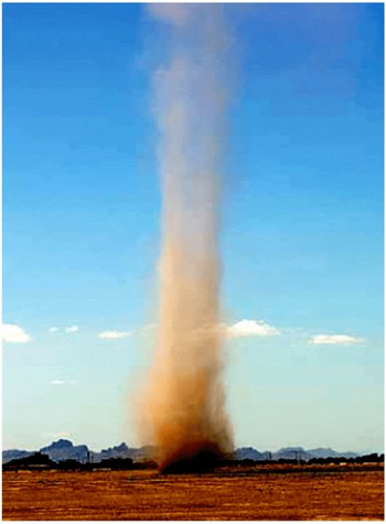
Buoyancy-induced, columnar vortices occur in the lowest part of the atmospheric boundary layer as a result of thermal instabilities of ground-heated, stratified air in areas with sufficient insolation. These buoyancy-induced vortices, often referred to as dust devils (figure 1), effectively convert the low-grade heat available in the air layer over the warm surface into a concentrated fluid motion with significant kinetic energy. Field investigations of naturally occurring dust devils reported vortices with diameters measuring up to 50 m that can extend as high as 1 km, with tangential and vertical wind speeds that can each exceed $50~\text{km h}^{-1}$ (Fitzjarrald Reference Fitzjarrald1973a ,Reference Fitzjarrald b ; Sinclair Reference Sinclair1973; Renno Reference Renno2004).

While the formation (or triggering) of the naturally occurring vortices requires a sufficiently large thermal stratification, the considerable kinetic energy contained within the vortex column cannot be accounted for by buoyancy alone (Carroll & Ryan Reference Carroll and Ryan1970). The axial fluxes of kinetic and thermal energy in the columnar vortex are at least an order of magnitude larger than the corresponding fluxes in non-rotating plumes that form under the same thermal conditions (Kaimal & Busigner Reference Kaimal and Busigner1970), and these increases are attributable to the presence of axial vorticity within the vortex core. As noted by Maxworthy (Reference Maxworthy1973), and later by Kanak, Lilly & Snow (Reference Kanak, Lilly and Snow2000), naturally occurring vortices can evolve from buoyant plumes by the appearance of concentrations of axial vorticity, although the origin of these vorticity concentrations is not well understood. One proposed mechanism was the presence of concentrated ambient, pre-existing eddies aided by wind shear (Morton Reference Morton1966), however, a number of investigators (Sinclair Reference Sinclair1969; Carroll & Ryan Reference Carroll and Ryan1970; Hess & Spillane Reference Hess and Spillane1990) have shown that naturally occurring dust devils can also form in near-calm conditions. Another mechanism that was proposed for formation of axial vorticity is tilting of ambient horizontal vorticity concentrations above the surface by near-surface wind (Maxworthy Reference Maxworthy1973). More recent investigations conjectured that the horizontal vorticity is produced near the surface by air motions within atmospheric convective cells (Kanak et al. Reference Kanak, Lilly and Snow2000; Kanak Reference Kanak2005), or baroclinically within the ground-plane boundary layer by a combination of thermal stratification and radial pressure gradients that are induced by these convective cells (Zhao et al. Reference Zhao, Gu, Yu, Ge, Li and Feng2004).

Figure 1.

Naturally occurring atmospheric buoyant column vortex, or dust devil, formed in a California desert (source: NASA).

Atmospheric vortices such as tornadoes (Snow Reference Snow1982; Brady & Szoke Reference Brady and Szoke1989; Varaksin, Romash & Kopeitsev Reference Varaksin, Romash and Kopeitsev2011; Rotunno Reference Rotunno2013) and waterspouts (Renno & Bluestein Reference Renno and Bluestein2001; Gaya et al. Reference Gaya, Homar, Romero and Ramis2001) have been thoroughly investigated. These more intense flows, while similarly scaled and dynamically related, derive their energy from latent heat transfer from the atmosphere and oceans, respectively, and not the sensible heat flux from the sun-heated ground. Numerical studies (Smith & Leslie Reference Smith and Leslie1976; Zhao et al. Reference Zhao, Gu, Yu, Ge, Li and Feng2004) and field measurements (Sinclair Reference Sinclair1969; Fitzjarrald Reference Fitzjarrald1973a ,Reference Fitzjarrald b ; Sinclair Reference Sinclair1973; Renno Reference Renno2004) of naturally occurring dust devils have provided significant insight into the structure of the vortex column and the flow dynamics. However, understanding of the vortex formation and sustainment mechanisms (Niino, Nakanishi & Tanaka Reference Niino, Nakanishi and Tanaka2006; Ohno & Takemi Reference Ohno and Takemi2010) and prediction of the vortex type and scale (Kurgansky Reference Kurgansky2006; Pathare et al. Reference Pathare, Balme, Meztger, Spiga, Towner and Renno2010) is still scant, and their dependence on the environmental conditions is not well understood (Ryan Reference Ryan1972; Kurgansky et al. Reference Kurgansky, Montecinos, Villagran and Metzger2011). To address these questions, several investigators have modelled the vortex flow with the goal of predicting its strength and scale, and have shown good agreement with existing field measurements (Barcilon Reference Barcilon1967a ,Reference Barcilon b ; Logan Reference Logan1971; Ryan Reference Ryan1972; Fiedler Reference Fiedler1998; Renno, Burkett & Larkin Reference Renno, Burkett and Larkin1998).

The present investigation is concerned with a variant of free, naturally occurring dust devil vortices, and focuses on buoyant columnar vortices that are deliberately triggered and anchored within open-top enclosures formed by azimuthal arrays of flow vanes with the ultimate objective of providing a thermomechanical link for harvesting low-grade waste heat in the solar-heated air by coupling the anchored vortex to a vertical axis turbine (e.g. Lucier Reference Lucier1981; Michaud Reference Michaud1999; Glezer & Simpson Reference Glezer and Simpson2014; Zhang et al. Reference Zhang, Luo, Li, Zhang, Meng, Kase, Wada, Yu and Gu2015). Deliberately triggered, buoyancy-induced anchored columnar vortices have been investigated in a few laboratory experiments using heated surfaces to mimic the solar-heated ground and an azimuthal array of flow vanes to impart tangential momentum to the entrained ambient air. Fitzjarrald (Reference Fitzjarrald1973a ,Reference Fitzjarrald b ) used such a set-up to measure distributions of the tangential velocity and temperature within the enclosure and observed different columnar vortex structures with up- and down-draft motion along the vortex centreline depending on the vane angle and plate temperature. In a later study, Mullen & Maxworthy (Reference Mullen and Maxworthy1977) measured distributions of the temperature and tangential velocity outside of the core of the columnar vortex and showed details of the formation of single- or two-cell vortex cores that are characterized by the absence and presence of down-draft axial flow along the axis of rotation depending on the swirl induced by the vanes. In a series of preliminary investigations, Simpson & Glezer (Reference Simpson and Glezer2012), Simpson, Pearlstein & Glezer (Reference Simpson, Pearlstein and Glezer2012, Reference Simpson, Pearlstein and Glezer2013a ), Simpson et al. (Reference Simpson, Reeve, Pearlstein and Glezer2013b ) used stereo particle image velocimetry and a similar experimental apparatus to study the formation of anchored columnar vortices with particular emphasis on scaling the induced flow field for the production of electric power. Baker (Reference Baker1981) investigated the swirling boundary layer of a columnar vortex induced by suction from above, and highlighted several features of the columnar vortices, including the development and growth of the spiraling momentum boundary layer. The surface pressure distributions induced by the swirling boundary layer were later measured in the experiments of Greeley et al. (Reference Greeley, Balme, Iversen, Metzger, Mickelson, Phoreman and White2003) with particular emphasis on the central stagnation point and its role in the transport of airborne particulates into the forming vortex. In a separate study using the same experimental set-up, Neakrase & Greeley (Reference Neakrase and Greeley2010) considered the effects of surface roughness on the formation of the suction-induced columnar vortices, and showed that the frictional velocity of the spiraling boundary layer can have a significant impact on the pressure deficit between the vortex core and the ambient.

Although naturally occurring and anchored buoyancy-induced vortices have been the subject of several earlier investigations, the fundamental mechanisms that govern their formation and sustainment are not fully understood. As noted above, current knowledge has mostly been pieced together from scant field data of naturally occurring vortices, and some earlier laboratory investigations that were primarily restricted to flow visualization studies (Mullen & Maxworthy Reference Mullen and Maxworthy1977). Therefore, the primary goals of the present experimental investigation are to elucidate and characterize in detail the formation and flow mechanisms of buoyancy-driven columnar vortices in controlled laboratory settings, with specific emphasis on the axial evolution of the vortex structure and on the production and advection of vorticity concentrations. As in most laboratory investigations of atmospheric flows, the present laboratory experiments clearly cannot match the characteristic formation parameters (e.g. Gr) of natural vortices nor do they include the effects of ambient air currents. Rather, the present experiments are designed to isolate crucial aspects of the formation and vorticity dynamics of the natural vortices in an experimental set-up that mimics the salient large-scale features and dynamics of the atmospheric flows (e.g. Morton Reference Morton1966; Cermak & Arya Reference Cermak and Arya1970; Maxworthy Reference Maxworthy1981).

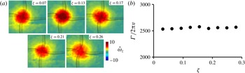
The time-averaged three-dimensional flow and temperature fields of the anchored vortex are measured in detail within the flow enclosure of the laboratory set-up using high-resolution stereo particle image velocimetry (SPIV) and thermocouple thermometry (§ 3). Using similarity analysis of the flow within the vortex column (§ 2), the structure, dynamics and distribution of momenta and kinetic energy flux of the inner and outer flow domains of the vortex column are described in § 4 (in good agreement with Kuo 1966). A detailed analysis of the flow dynamics of the ground-plane boundary layer is included in § 5, with emphasis on vorticity dynamics and vortex sustainment mechanism. It is shown that horizontal vorticity produced within the spiraling ground-plane boundary layer is tilted by horizontal velocity gradients induced by the buoyant instability along the flow’s centreline to form the axial vorticity within the core of a columnar vortex. This mechanism, which is in agreement with conjectures of earlier investigators, can be sustained as long as surface heating is present, even in the absence of ambient eddies or wind shear.

2 Dimensional considerations

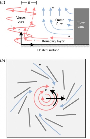
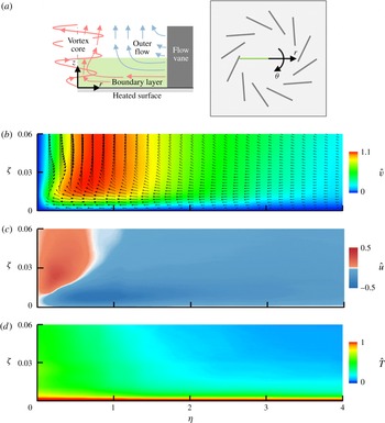
The three-dimensional flow field of a single-cell stationary, columnar vortex (Mullen and Maxworthy 1977) that forms above a heated surface within an enclosure bounded by an azimuthal array of stator-like vertical flow vanes consists of three primary, coupled domains (figure 2): (i) spiraling momentum and surface thermal boundary layers that advect heated air and vorticity into the core of the columnar vortex; (ii) an inner, thermally driven vertical vortex core; and (iii) an outer annular flow that is bounded by a helical shear layer and the vanes along its inner and outer edges, respectively, and by the spiraling boundary layer from below. Azimuthally entrained, surface-heated ambient air within and above the boundary layer sustains the vortex and acquires tangential momentum as it passes through the vanes. As conjectured by Rotunno (Reference Rotunno1980), the spiraling wall boundary layer that is entrained through the azimuthal array of vanes concentrates horizontal vorticity into an initial thermal plume, where it is buoyantly tilted vertically to form the axial vorticity within the core of a columnar vortex. Once rotation begins, the columnar vortex is strengthened and sustained by the generation of additional radial vorticity within the boundary layer that is continuously advected towards the centreline and tilted axially by the buoyancy-driven air motions. As noted in § 1, this formation mechanism requires only sufficient surface heating to trigger the buoyant instability, without the need for ambient eddies or wind shear and is sustained as long as heating continues.

Figure 2.

Schematic representation of the location of the three primary domains of the buoyancy-induced flow field in the ( $a$ ) $r$ – $z$ and ( $b$ ) $r$ – $\unicode[STIX]{x1D703}$ planes with experimental coordinate frame ( $r$ , $\unicode[STIX]{x1D703}$ , $z$ ) and velocity field ( $u$ , $v$ , $w$ ).

The flow domain is described using cylindrical coordinates $(r,\unicode[STIX]{x1D703},z)$ such that the $z$ -axis is coincident with the centreline of the columnar vortex, and the corresponding velocity field is denoted by $\boldsymbol{V}=(u,v,w)$ . Using the Boussinesq approximation, variations in fluid properties due to temperature are assumed to be small and are neglected, except when they contribute to buoyancy effects. Following the formulation of Rajaratnam (Reference Rajaratnam1976) for a free axisymmetric swirling jet, the axisymmetric continuity and radial and axial momentum equations that describe the vertical flow near the centreline and sufficiently far from the ground plane are given by:

(2.1)

$$\begin{eqnarray}\displaystyle & \displaystyle \frac{\unicode[STIX]{x2202}(ru)}{\unicode[STIX]{x2202}r}+\frac{\unicode[STIX]{x2202}(rw)}{\unicode[STIX]{x2202}z}=0 & \displaystyle\end{eqnarray}$$

(2.2)

$$\begin{eqnarray}\displaystyle & \displaystyle \frac{v^{2}}{r}=\frac{1}{\unicode[STIX]{x1D70C}}\frac{\unicode[STIX]{x2202}P}{\unicode[STIX]{x2202}r} & \displaystyle\end{eqnarray}$$

(2.3)

$$\begin{eqnarray}\displaystyle & \displaystyle u\frac{\unicode[STIX]{x2202}w}{\unicode[STIX]{x2202}r}+w\frac{\unicode[STIX]{x2202}w}{\unicode[STIX]{x2202}z}=-\frac{1}{\unicode[STIX]{x1D70C}}\frac{\unicode[STIX]{x2202}P}{\unicode[STIX]{x2202}z}+g^{\prime }+\frac{1}{\unicode[STIX]{x1D70C}r}\frac{\unicode[STIX]{x2202}(r\unicode[STIX]{x1D70F}_{rz})}{\unicode[STIX]{x2202}r}, & \displaystyle\end{eqnarray}$$

with the addition of the adjusted gravitational acceleration or weight deficiency, $g^{\prime }=((\unicode[STIX]{x1D70C}_{\infty }-\unicode[STIX]{x1D70C}(r,z))/\unicode[STIX]{x1D70C}_{\infty })g$ ( $g$ , the gravitational acceleration and $\unicode[STIX]{x1D70C}_{\infty }$ , the ambient air density, are constant) to account for the effects of buoyancy (Turner Reference Turner1973) and $\unicode[STIX]{x1D70F}_{rz}=\unicode[STIX]{x1D707}(\unicode[STIX]{x2202}w/\unicode[STIX]{x2202}r)$ is the shear stress.

The axial momentum equation (2.3) can be rewritten, using the continuity equation (2.1), multiplying through by $\unicode[STIX]{x1D70C}r$ , and integrating with respect to $r$ from 0 to $\infty$ using the boundary conditions $u(0,z)=0$ , $u(\infty ,z)=0$ and $\unicode[STIX]{x1D70F}_{rz}(\infty ,z)=0$ to produce

(2.4)

$$\begin{eqnarray}\frac{\text{d}}{\text{d}z}\int _{0}^{\infty }(\unicode[STIX]{x1D70C}w^{2}+P)r\,\text{d}r=\int _{0}^{\infty }\unicode[STIX]{x1D70C}g^{\prime }r\,\text{d}r.\end{eqnarray}$$

Based on the radial momentum equation (2.2) the pressure term in equation (2.4) can be rewritten in terms of the tangential velocity using the boundary conditions $(\unicode[STIX]{x2202}p/\unicode[STIX]{x2202}z)(r\rightarrow \infty ,z)=0$ and that $(\unicode[STIX]{x2202}p/\unicode[STIX]{x2202}z)(0,z)$ is finite,

(2.5)

$$\begin{eqnarray}\displaystyle & & \displaystyle \int _{0}^{\infty }\frac{\unicode[STIX]{x2202}p}{\unicode[STIX]{x2202}z}r\,\text{d}r=\left|\frac{r^{2}}{2}\frac{\unicode[STIX]{x2202}p}{\unicode[STIX]{x2202}z}\right|_{0}^{\infty }-\int _{0}^{\infty }\frac{r^{2}}{2}\frac{\unicode[STIX]{x2202}}{\unicode[STIX]{x2202}r}\left(\frac{\unicode[STIX]{x2202}p}{\unicode[STIX]{x2202}z}\right)\text{d}r\nonumber\\ \displaystyle & & \displaystyle \quad =-\int _{0}^{\infty }\frac{r^{2}}{2}\frac{\unicode[STIX]{x2202}}{\unicode[STIX]{x2202}z}\frac{\unicode[STIX]{x2202}p}{\unicode[STIX]{x2202}r}\,\text{d}r=-\int _{0}^{\infty }\frac{r^{2}}{2}\frac{\unicode[STIX]{x2202}}{\unicode[STIX]{x2202}z}\left(\frac{\unicode[STIX]{x1D70C}v^{2}}{r}\right)\text{d}r\end{eqnarray}$$

and therefore the axial momentum within the vortex column becomes

(2.6)

$$\begin{eqnarray}\frac{\text{d}}{\text{d}z}\int _{0}^{\infty }\unicode[STIX]{x1D70C}\left(w^{2}-\frac{1}{2}v^{2}\right)r\,\text{d}r=\int _{0}^{\infty }\unicode[STIX]{x1D70C}g^{\prime }r\,\text{d}r.\end{eqnarray}$$

Equation (2.6) shows that the axial momentum flux through the vortex core varies with elevation as long as the local weight deficiency, $g^{\prime }$ , does not vanish. Furthermore, since the integrand of the integral on the right-hand side of (2.6) is positive definite, in the absence of viscous effects the axial momentum flux must increase with elevation.

As the vortex structure evolves above the heated surface, the formation of a helical shear layer between the thermally driven core (ii) and the outer flow (iii) results in radial entrainment of ambient air along the periphery of the vortex column. Following the approach formulated by Morton, Taylor & Turner (Reference Morton, Taylor and Turner1956) for thermal plumes, this entrainment is modelled as the time-averaged radial inflow at the edge of the vortex core that, at some elevation, well above the ground-plane boundary layer, is taken to be proportional to the local characteristic vertical velocity, $u_{e}=\unicode[STIX]{x1D6FC}\bar{w}$ (i.e. the radial distribution of the axial velocity is characterized by the radius of the vortex core $R$ denoted in figure 2). Using this relationship, the continuity (2.1) defines a ray that coincides with the edge of the vortex core and emanates from an imaginary source beneath the heated surface along which

(2.7)

$$\begin{eqnarray}\frac{R}{z}\sim \left.\frac{u_{e}}{\bar{w}}\right|_{r=R}=\unicode[STIX]{x1D6FC},\end{eqnarray}$$

where the entrainment coefficient, $\unicode[STIX]{x1D6FC}$ , (Taylor Reference Taylor1945) is proportional to the rate of entrainment of ambient air at the edge of vortex core. This coefficient is ubiquitous in the analysis of thermal plumes for quantifying the axial variation of radial entrainment due to mixing along the peripheral edge of the flow (Turner Reference Turner1962, Reference Turner1969; van den Bremer & Hunt Reference van den Bremer and Hunt2014). Equation (2.7) indicates that the radial extent of the vortex core is linearly proportional to elevation and this proportionality is used to define dimensionless similarity coordinates for the vortex flow.

The buoyancy-induced columnar vortex may be thought of as a ‘superposition’ of a momentum-driven, swirling jet and a non-rotating, thermal plume, and therefore it stands to reason that the flow field of the vortex should also have corresponding similarity characteristics. The dependence of the velocity and weight deficiency distributions on the similarity variables $\unicode[STIX]{x1D702}=r/R$ and $\unicode[STIX]{x1D701}=\unicode[STIX]{x1D6FC}z/R$ above the boundary layer (demonstrated experimentally in § 4.2) allows these distributions to be written as

(2.8)

$$\begin{eqnarray}\displaystyle \left.\begin{array}{@{}c@{}}w(r/R,\unicode[STIX]{x1D6FC}z/R)=w(1,\unicode[STIX]{x1D701})f(\unicode[STIX]{x1D702})\\ v(r/R,\unicode[STIX]{x1D6FC}z/R)=v(1,\unicode[STIX]{x1D701})h(\unicode[STIX]{x1D702})\\ g^{\prime }(r/R,\unicode[STIX]{x1D6FC}z/R)=g^{\prime }(0,\unicode[STIX]{x1D701})m(\unicode[STIX]{x1D702}),\end{array}\right\} & & \displaystyle\end{eqnarray}$$

where $R(z)$ is the radial location at which the tangential velocity has a maximum and denotes the characteristic radius of the vortex core. The radial and axial velocities are scaled by their respective maximum values at $\unicode[STIX]{x1D702}=1$ ( $r=R$ ) and the weight deficiency is scaled by its value at the vortex centreline ( $\unicode[STIX]{x1D702}=0$ ). As noted above, the radial variations of $f(\unicode[STIX]{x1D702})$ , $h(\unicode[STIX]{x1D702})$ and $m(\unicode[STIX]{x1D702})$ are obtained experimentally. The axial momentum equation (2.6) can be rewritten in similarity form using (2.8) as

(2.9)

$$\begin{eqnarray}\displaystyle \frac{\unicode[STIX]{x1D6FC}}{R}\frac{\text{d}}{\text{d}\unicode[STIX]{x1D701}}\int _{0}^{\infty }\unicode[STIX]{x1D70C}\left[w(1,\unicode[STIX]{x1D701})^{2}f(\unicode[STIX]{x1D702})^{2}-\frac{1}{2}v(1,\unicode[STIX]{x1D701})^{2}h(\unicode[STIX]{x1D702})^{2}\right]R^{2}\unicode[STIX]{x1D702}\,\text{d}\unicode[STIX]{x1D702}=\int _{0}^{\infty }\unicode[STIX]{x1D70C}g^{\prime }(0,\unicode[STIX]{x1D701})m(\unicode[STIX]{x1D702})R^{2}\unicode[STIX]{x1D702}\,\text{d}\unicode[STIX]{x1D702}. & & \displaystyle \nonumber\\ \displaystyle & & \displaystyle\end{eqnarray}$$

At each axial elevation the coefficients of the similarity parameters are invariant and the axial momentum equation (2.8) can be written for a specific elevation $\unicode[STIX]{x1D701}=Z$ as

(2.10)

$$\begin{eqnarray}\frac{\text{d}}{\text{d}\unicode[STIX]{x1D701}}\int _{0}^{\infty }[2f(\unicode[STIX]{x1D702})^{2}-S(Z)^{2}h(\unicode[STIX]{x1D702})^{2}]\unicode[STIX]{x1D702}d\unicode[STIX]{x1D702}=[Fr(Z)]^{-2}\int _{0}^{\infty }m(\unicode[STIX]{x1D702})\unicode[STIX]{x1D702}\,\text{d}\unicode[STIX]{x1D702},\end{eqnarray}$$

where the swirl number $S(Z)=v(1,Z)/w(1,Z)$ is the ratio of the tangential and axial velocity components at the core radius, and $Fr(Z)=([\unicode[STIX]{x1D6FC}w^{2}(1,Z)]/[2g^{\prime }R(Z)])^{1/2}$ is an adjusted Froude number that measures the ratio of the axial kinetic energy to the buoyant, gravitational potential energy in the buoyancy-driven flow. In the two limits, $Fr=0$ when $w=0$ characterizes stratified but motionless fluid and $Fr\rightarrow \infty$ when the flow is purely momentum driven. In the latter limit, (2.10) describes the flow of an isothermal, swirling jet. The tangential velocity at $\unicode[STIX]{x1D702}=1$ ( $r=R$ ) can be expressed in terms of the angular velocity of the solid-body rotation of the vortex core, $\unicode[STIX]{x1D6FA}$ , so the swirl number is rewritten as $S(Z)=(\unicode[STIX]{x1D6FA}R)/w(1,Z)$ . In the present investigation, the vortex strength is described by the core Reynolds number, $Re=\unicode[STIX]{x1D6E4}_{z}/(2\unicode[STIX]{x03C0}\unicode[STIX]{x1D708})$ where $\unicode[STIX]{x1D6E4}_{z}$ is the axial circulation of the vortex column obtained from PIV measurements and $\unicode[STIX]{x1D708}$ is the kinematic viscosity.

Figure 3.

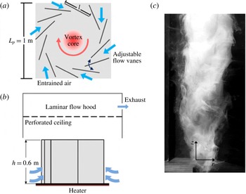
The buoyancy-induced, columnar vortex facility: (a,b) top and side views of experimental set-up showing heated surface, adjustable azimuthal flow vanes, and laminar flow hood with schematic representation of entrainment and vortex core and ( $c$ ) smoke visualization of the laboratory vortex (the image field of view measures $20~\text{cm}\times 45~\text{cm}$ ).

3 Experimental methodology

The laboratory investigations of the formation and evolution of a stationary (anchored) buoyancy-driven columnar vortex are conducted in a metre-scale facility (figure 3). The vortex is centred above a heated ground plane and the flow is described using a cylindrical $(r,\unicode[STIX]{x1D703},z)$ coordinate system as shown in figure 2(a,b) (the $z$ -axis coincides with the centreline of the column vortex, as shown in figure 3(c)). Ground heating is simulated by a planar square (1 $\text{m}^{2}$ ) 4.8 kW controllable heater that is attached to the bottom surface of a 2 cm thick square aluminium plate measuring $L_{p}=1$ m on the side. The power delivered to the heated surface is maintained using a proportional–integral–derivative (PID) controller based on temperature measurements of a radial array of thermocouples embedded within the aluminium plate at a 1.0 mm depth from the upper surface, while the ‘ambient’ air temperature is controlled using the laboratory ventilation system. The surface temperature, $T_{p}$ , is adjustable from ambient to $150\,^{\circ }\text{C}$ producing a maximum Grashof number of $12\times 10^{7}$ , where $Gr=[g\unicode[STIX]{x1D6FD}(T_{p}-T_{\infty })L^{3}]/\unicode[STIX]{x1D708}^{2}$ , $g$ is the gravitational acceleration, $\unicode[STIX]{x1D6FD}$ is the coefficient of thermal expansion, $L=A/P=L_{p}/2$ is the hydraulic diameter of the heated surface, $\unicode[STIX]{x1D708}$ is the kinematic viscosity and fluid properties are calculated based on the film temperature, $T_{film}=0.5(T_{p}+T_{\infty })$ . The Grashof number of the present experiments is sufficiently large such that the transfer of thermal energy from the laboratory heated surface into the air is dominated by natural convection, and therefore the heat flux into the air is approximated to be nominally invariant over the entire surface. Based on thermal boundary layer profiles, measured at multiple radial stations within the vane enclosure and its periphery for $T_{p}=100\,^{\circ }\text{C}$ , the estimated heat flux, $q^{\prime \prime }=-k\,(\text{d}T/\text{d}z)|_{z=0^{+}}$ , from the plate into the air is nominally $450~\text{W m}^{-2}$ , similar to the measured sensible heat flux (350–400 $\text{W m}^{-2}$ ) from the ground into the adjacent air layers at midday in desert-type environments. The entrained flow is directed through an azimuthal array of twelve adjustable vanes ( $l=35~\text{cm}\times h=60~\text{cm}$ , 1.5 mm thick) distributed azimuthally around the centre of the plate. Each vane is hinged 28 cm from its inner edge at a radius of 46 cm (relative to the centreline), and imparts angular momentum to the air flow that is entrained by the central, buoyancy-driven vortex. The vane angle can be varied in the range $0^{\circ }<\unicode[STIX]{x1D719}<60^{\circ }$ where $\unicode[STIX]{x1D711}$ is measured relative to the inward radial direction. The rising air is captured using an adjustable laminar flow hood with minimal disturbance to the anchored vortex flow (figure 3 b). Smoke visualization of the self-sustained vortex core is shown in figure 3(c). Depending on the experimental parameters, the vortex can have a core diameter, $2R$ , varying from 5 and 25 cm and, in the absence of the laminar flow hood, a height of as much as 3 m.

Radial temperature distributions of the core of the vortex and outer flow are measured using an array of miniature thermocouple sensors that was constructed especially for the present investigations. The array comprises thermocouple sensors that are each mounted within a 1.6 mm diameter, 19 mm long stainless steel tube. The sensors are mounted along the leading edge of a symmetric stainless steel airfoil tube (having maximum thickness of 9.5 mm) that houses the sensors wiring and is placed in the vortex flow field. While the presence of the thermocouple array clearly has some effect on the local flow, its low form factor and small scale relative to the scale of the facility, and the care that was exercised in its placement within the facility are deemed sufficient to yield thermal measurements that are very close to the undisturbed flow. Measurements at multiple elevations are obtained using a rake of 16 thermocouple sensors, spaced 1 cm apart for $r\leqslant 8$ cm and 2 cm apart for $r>8$ cm. Boundary layer temperature distributions are measured at multiple radial stations using a vertical rake of 9 thermocouple sensors equally spaced 3 mm apart within $0\leqslant z\leqslant 24$ mm. The temperature data are sampled at 10 Hz and time averaged over 6000 samples.

The three-dimensional flow field within the vortex enclosure is measured using high-resolution SPIV in horizontal ( $r$ – $\unicode[STIX]{x1D703}$ ) and vertical ( $r$ – $z$ ) planes using two identical $1600\times 1200$ pixel, 14-bit charge-coupled device (CCD) cameras. The cameras are arranged in an angular displacement configuration in which their optical axes intersect at a set angle ( $40^{\circ }$ in the present experiments) such that its bisector is normal to the two co-planar overlapping imaging planes. The image distortion caused by the angular deflection of the optical axis of each camera relative to the bisector is corrected using a Scheimpflug adapter. The image captured by each camera is corrected using a three-dimensional gridded calibration target ( $20~\text{cm}\times 20~\text{cm}$ with $\unicode[STIX]{x0394}x=\unicode[STIX]{x0394}y=2$ cm spacing). Both cameras are mounted on the same side of the laser sheet and a mapped-stereo algorithm using a pin-hole calibration method is used to determine image distance from each camera sensor for calculation of the velocity field. The ambient flow (outside of the array vanes) is seeded using a glycol–water theatrical fog so that particles are entrained naturally into the vane enclosure. The measurements are acquired using a 180 mJ Nd:YAG laser with nominal laser sheet thickness of 1.5 mm and repetition frequency of 10 Hz. The measurements in a horizontal ( $r$ – $\unicode[STIX]{x1D703}$ ) plane are acquired using 35 mm lenses producing a planar measurement domain of $320\times 241$ mm with a spatial resolution of 4.98 pixels per mm. Using an interrogation window of $32\times 32$ pixels the spatial resolution provides particle density of 15–25 particles per interrogation window. Similarly, the measurements in a vertical ( $r$ – $z$ ) plane are acquired using 105 mm lenses producing a planar measurement domain of $89.5\times 67$ mm and spatial resolution of 17.9 pixels per mm. All PIV data are time averaged and include 750 individual image pairs to provide sufficient data to allow temporal convergence. The spatial average of the root mean square deviation of pixel displacement corresponding to the three velocity components is computed within the outer flow where the characteristic velocity fluctuations are reasonably small, and is found to be 0.208 pixels. This residual displacement is used to estimate an upper bound of 4.1% on the error in the magnitude of each velocity component measured in the current SPIV configuration. It should be noted that this error accounts for uncertainties that are associated with both the measurement errors and the inherent velocity fluctuations.

Velocity data are computed from the PIV images using a commercial algorithm (DaVis 8.1.6). The vortex core in each horizontal ( $r$ – $\unicode[STIX]{x1D703}$ ) plane is offset relative to the centre of the image to extend the radial domain of the measurements. The vortex centreline ( $r=0$ ) is located by using a cross-correlation of the velocity magnitude $(u^{2}+v^{2}+w^{2})^{1/2}$ , which has a local minimum along the vortex centreline, with the second eigenvalue $(\unicode[STIX]{x1D706}_{2})$ of the symmetric tensor $(\overline{\overline{\unicode[STIX]{x1D6EC}}}^{2}+\overline{\overline{\unicode[STIX]{x1D714}}}^{2})$ where $\overline{\overline{\unicode[STIX]{x1D6EC}}}$ and $\overline{\overline{\unicode[STIX]{x1D714}}}$ are the rate of strain and vorticity tensors respectively. This eigenvalue locates the pressure minimum in a two-dimensional plane (the $\unicode[STIX]{x1D706}_{2}$ -criterion, Jeong & Hussain Reference Jeong and Hussain1995; Haller Reference Haller2005). The locations of the minima from these calculations are compared to identify the vortex centreline and the data are mapped from the measurement coordinate frame ( $x$ , $y$ ) to a polar grid ( $r$ , $\unicode[STIX]{x1D703}$ ) centred about the vortex centreline. Radial distributions of the velocity vector, $\boldsymbol{V}=(u,v,w)$ , are obtained using an azimuthal average from $-\unicode[STIX]{x03C0}/12$ to $\unicode[STIX]{x03C0}/12$ , to account for the 12-fold symmetry associated with the array of flow vanes and $\unicode[STIX]{x1D703}=0^{\circ }$ is prescribed as the azimuthal location which provides the shortest distance between the vortex centreline ( $r=0$ ) and the right edge of the ground plane. The components of the vorticity vector $(\unicode[STIX]{x1D74E}=(\unicode[STIX]{x1D714}_{r},\unicode[STIX]{x1D714}_{\unicode[STIX]{x1D703}},\unicode[STIX]{x1D714}_{z})=(-\unicode[STIX]{x2202}v/\unicode[STIX]{x2202}z,\unicode[STIX]{x2202}u/\unicode[STIX]{x2202}z-\unicode[STIX]{x2202}w/\unicode[STIX]{x2202}r,r^{-1}\unicode[STIX]{x2202}(rv)/\unicode[STIX]{x2202}r))$ normal to the measurement planes $r$ – $\unicode[STIX]{x1D703}$ and $r$ – $z$ , $\unicode[STIX]{x1D714}_{\text{z}}$ and $\unicode[STIX]{x1D714}_{\unicode[STIX]{x1D703}}$ respectively, are calculated using the circulation about each grid point (Raffel et al. Reference Raffel, Willert, Wereley and Kompenhans2007). Vorticity components in the $r$ – $\unicode[STIX]{x1D703}$ and $r$ – $z$ planes [ $(\unicode[STIX]{x1D714}_{r},\unicode[STIX]{x1D714}_{\unicode[STIX]{x1D703}})$ and $(\unicode[STIX]{x1D714}_{r},\unicode[STIX]{x1D714}_{z})$ , respectively] are calculated using a second-order, central difference method where azimuthal derivatives are neglected and out-of-plane gradients are calculated using parallel measurement planes when available. The near-surface SPIV measurements of the boundary layer in the $r$ – $z$ plane are constructed from four, partially overlapping separate measurement windows and the vortex centreline ( $r=0$ ) is determined by finding the minimum magnitude of the horizontal velocity component $(u^{2}+v^{2})^{1/2}$ .

It should be noted that in the present experiments the turbulent characteristics of the vortex core (e.g. distributions of the Reynolds stresses) cannot be assessed from the time-averaged flow field owing to inherent instantaneous lateral spatial and temporal jitter of the core. Absent simultaneous measurements of an entire segment of the vortex that also includes its centreline either in the $r$ – $\unicode[STIX]{x1D703}$ or $z$ – $r$ planes, this jitter makes it impossible to distinguish between turbulent fluctuations and natural lateral motion of the core. Therefore, conventional estimates of the Reynolds stresses based on the time-averaged velocity field would be overestimated in terms of magnitude and spatial extent and are not included in the present data analysis.

As described by Fitzjarrald (Reference Fitzjarrald1973a ) and Mullen & Maxworthy (Reference Mullen and Maxworthy1977), (cf. § 1), the columnar vortex can develop a two-cell structure when a down-draft cell forms along its axis of rotation as a result of forced changes to the radial entrainment into the vortex core. While a single-cell vortex in characterized by up-draft flow throughout its core and a central stagnation point at the intersection of the axis of rotation with the ground plane, in a two-cell vortex a helical domain of axial down-draft forms along the axis of rotation and is surrounded by helical up-draft flow. Similar to the earlier observations, the present facility can form single- or two-cell columnar vortices by regulation of the entrained flow through the azimuthal vertical vanes and of the thermal resources. For given thermal resources, a single-cell (up-draft) vortex typically forms at small vane angles in which the tangential momentum of the entrained flow and pressure drops across the vane array are low. At moderate vane angles, the angular velocity of the vortex core increases and the spacing between adjacent vanes decreases, resulting in a larger pressure drop that limits entrainment into the enclosure. Both effects lead to a reduction in the rotation-induced pressure within the core of the vortex, increasing the magnitude of the axial pressure gradient along the centreline and leading to the formation of a two-cell vortex. Finally, when the vane angle is sufficiently large, the down-draft cell extends to the ground plane and the stagnation point that forms on the flow axis between the two cells migrates towards, and attaches to, the heated surface.

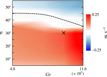
A transition map of the vortex structure in the present laboratory facility is constructed in terms of $\unicode[STIX]{x1D711}$ and $Gr~(5^{\circ }<\unicode[STIX]{x1D711}<55^{\circ },4.8\times 10^{7}\leqslant Gr\leqslant 11.6\times 10^{7})$ using a colour raster plot of the time-averaged centreline ( $r=0$ ) axial velocity $\bar{w}$ at $z/h=0.17$ above the heated surface (figure 4). The detached stagnation point at the interface between the upward and downward flow on the centreline is marked by $\bar{w}=0$ (shown using a dashed contour). When $\bar{w}>0$ the vortex at this elevation is single cell and when $\bar{w}<0$ the vortex is two cell. Flow visualization and measurements demonstrated that for $\unicode[STIX]{x1D711}\leqslant 30^{\circ }$ the single-cell core structure is maintained throughout the height of the vane array, and their structure and spatial evolution are the primary focus of the present paper.

Figure 4.

Transition map of the vortex cell structure using colour raster plots of the variation with $\unicode[STIX]{x1D711}$ and $Gr$ of the time-averaged axial velocity $\bar{w}$ ( $b$ , $c$ ) at $r=0$ at $z/h=0.17$ . The location of $\bar{w}=0$ is denoted with dashed lines. The nominal single-cell vortex that is the focus of the present investigation is marked by ‘ $\times$ ’.

4 The structure of the columnar vortex

The flow field of the buoyancy-induced vortex is separated into two primary domains, namely the vortex column, consisting of the core and surrounding outer flow and the momentum and thermal boundary layers near the heated surface. In this section, the flow field of the vortex column is characterized, while the flow structure within the ground-plane boundary layer is described in § 5.

Figure 5.

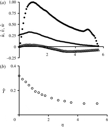
Time-averaged radial distributions of the nominal vortex at $\unicode[STIX]{x1D701}=0.12$ ( $z=10$ cm): ( $a$ ) normalized tangential (●), axial (♦) and radial (▵) velocity components and ( $b$ ) normalized temperature (○) within the vortex column.

4.1 Radial structure of the vortex column

The evolution of the vortex core is first explored well above the surface layer at an elevation of $z=10$ cm, ( $z/h=0.17$ , $\unicode[STIX]{x1D701}=0.12$ ). Velocity measurements in the $r$ – $\unicode[STIX]{x1D703}$ plane show that the nominal vortex ( $\unicode[STIX]{x1D711}=30^{\circ }$ , $Gr=9.7\times 10^{7}$ ) has a core angular velocity $\unicode[STIX]{x1D6FA}=15~\text{s}^{-1}$ , core radius $R=4.5$ cm. Time- and azimuthally averaged radial distributions of the tangential ( $\hat{v}$ ), radial ( $\hat{u}$ ) and axial ( ${\hat{w}}$ ) velocity components (normalized by $\unicode[STIX]{x1D6FA}\cdot R$ ) and air temperature $\hat{T}=(T-T_{\infty })/(T_{p}-T_{\infty })$ ( $T_{\infty }$ is the laboratory ambient) are shown in figure 5(a,b). Note that each distribution extends radially past the inner vertical edge of the vanes ( $\unicode[STIX]{x1D702}=5.44$ ), into the space between adjacent vanes to $\unicode[STIX]{x1D702}=5.66$ (cf. figure 3).

The base flow is dominated by the (clockwise, as viewed from above) tangential velocity which at $\unicode[STIX]{x1D702}=1$ is 3.2 and 27 times as large as ${\hat{w}}$ and $\hat{u}$ , respectively. Within the inner vortex core ( $\unicode[STIX]{x1D702}<0.5$ ), the tangential velocity varies nearly linearly, with $\unicode[STIX]{x1D702}$ resembling solid-body rotation and then begins to level off before reaching its maximum (at $\unicode[STIX]{x1D702}=1$ ), followed by a monotonic decay similar to a potential vortex ( $\hat{v}\propto \unicode[STIX]{x1D702}^{-1}$ ). The presence of a wall jet of entrained flow emanating from each azimuthal flow vane is evident within the domain $4.5<\unicode[STIX]{x1D702}<5.7$ leading to a local maximum of the tangential velocity at $\unicode[STIX]{x1D702}=4.9$ . When $\unicode[STIX]{x1D702}<4.5$ , the structure of the anchored vortex is similar to that of a free, unbounded columnar vortex. The wall jet imparts angular momentum into the outer flow and disrupts the monotonic decrease of $\hat{v}$ near the inner edge of the vane array. Therefore, the tangential velocity within the outer flow of the columnar vortex is simultaneously affected by the angular momentum of its inner core ( $\unicode[STIX]{x1D702}<1$ ) and of the entrained flow through the vanes ( $\unicode[STIX]{x1D702}>4.5$ ). The axial velocity component ${\hat{w}}$ is positive throughout the measurement domain, and has a local maximum at $\unicode[STIX]{x1D702}=0.85$ , slightly within the vortex core, and a local minimum at $\unicode[STIX]{x1D702}=0$ . The axial velocity decays within the outer flow near the inner edge of the vanes, so that the tangential entrainment jet is nominally two-dimensional. The radial velocity component $\hat{u}$ is an order of magnitude smaller than $\hat{v}$ and ${\hat{w}}$ and changes sign at $\unicode[STIX]{x1D702}=$ 1.8, such that $\hat{u} >0$ for $\unicode[STIX]{x1D702}<1.8$ indicates the radial spreading of the vortex core, and $\hat{u} <0$ for $\unicode[STIX]{x1D702}>1.8$ denotes inward radial entrainment of fluid. Based on the distribution of the tangential velocity component and the time-averaged location at which $\hat{u} =0$ , it is argued that the annular domain $1<\unicode[STIX]{x1D702}<1.8$ is a transition region through the helical shear layer between the inner vortex core, which undergoes solid-body rotation, and the outer flow, which is characteristic of a potential vortex. Therefore, $\unicode[STIX]{x1D702}=1.8$ , where $\hat{u} =0$ , marks the time- and azimuthally averaged radial division between the spreading vortex column and the outer flow.

Figure 5(b) shows the radial temperature distribution within the vortex column measured using the radial array of thermocouple sensors (cf. § 2). For the surface temperature of $T_{p}=100\,^{\circ }\text{C}$ ( $\hat{T}=1$ ), the maximum air temperature, located at the vortex centreline ( $\unicode[STIX]{x1D702}=0$ , $\unicode[STIX]{x1D701}=0.12$ ), is $47.6\,^{\circ }\text{C}$ ( $\hat{T}=0.32$ ) and the largest radial thermal gradients lie within the vortex core and the annular transition domain ( $0<\unicode[STIX]{x1D702}<1.8$ ). Within the outer flow, the temperature continues to decrease and approaches a minimum of $\hat{T}=0.09$ at $\unicode[STIX]{x1D702}=5.31$ . The elevated temperature at this radial location, compared to the laboratory ambient, indicates that within the vane enclosure significant mixing occurs between surface-heated air that rises into the vortex core and spreads radially, warm (but cooler) air advected from the outer edge of the surface thermal boundary layer, and ambient air (at approximately $\hat{T}=0$ ) entrained through the flow vanes above the boundary layer.

The radial pressure gradient induced by the rotation of the vortex core and outer flow is computed from the measured three-dimensional flow field using a second-order central finite difference approximation of the radial Navier–Stokes equation in cylindrical coordinates following the procedure of Honohan (Reference Honohan2003) and Liu & Katz (Reference Liu and Katz2006). In these calculations, the spatial resolution is limited by the SPIV measurements ( $\unicode[STIX]{x0394}x=\unicode[STIX]{x0394}y=3.2$ mm) yielding $\unicode[STIX]{x0394}\unicode[STIX]{x1D702}=0.07$ at $\unicode[STIX]{x1D701}=0.12$ . It is assumed that the axial gradient of the radial velocity $\unicode[STIX]{x2202}u/\unicode[STIX]{x2202}z$ is negligible and fluid properties are axisymmetric and depend only on the local temperature, measured using a radial array of thermocouple sensors (cf. § 3) and interpolated onto the SPIV grid. The Reynolds stresses are estimated from the instantaneous SPIV data. 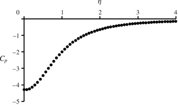These data show that the radial pressure gradient, $\unicode[STIX]{x2202}\hat{p}/\unicode[STIX]{x2202}\unicode[STIX]{x1D702}$ , increases monotonically with $\unicode[STIX]{x1D702}$ from 0 at the centreline to a local maximum at $\unicode[STIX]{x1D702}=0.65$ , and decreases asymptotically to zero near the edge of the measurement domain. The measured tangential velocity is used to approximate the pressure at the radial edge of the measurement domain using (2.2) and the radial pressure gradient is integrated using this boundary condition to yield the radial pressure distribution, $C_{p}(\unicode[STIX]{x1D702})=\unicode[STIX]{x0394}p/([\unicode[STIX]{x1D70C}_{f}(\unicode[STIX]{x1D6FA}R)^{2}]/2)$ (figure 6), where density, $\unicode[STIX]{x1D70C}_{f}$ , is defined using the film temperature ( $T_{f}$ , cf. § 3) and $\unicode[STIX]{x1D6FA}$ and $R$ are the angular velocity and radius of the vortex core at $\unicode[STIX]{x1D701}=0.12$ , respectively. The minimum pressure occurs at the vortex centreline, and monotonically increases with increasing $\unicode[STIX]{x1D702}$ , asymptotically approaching $C_{p}=-0.25$ at $\unicode[STIX]{x1D702}=4$ . $C_{p}$ does not vanish within the vane enclosure [ $p(\unicode[STIX]{x1D702}=5.44)<p_{\infty }$ ] due to the pressure imposed by the array of flow vanes as a result of the induced tangential velocity component of the entrained flow. Therefore, in addition to the global length scale, the vanes also impose a pressure boundary condition at $r=R_{i}$ that intensifies the low pressure along the centreline of the anchored vortex. We note in passing that for atmospheric vortices with sufficiently large Rossby numbers ( $Ro=U/(Lf)=\unicode[STIX]{x1D6FA}/f$ , where $\unicode[STIX]{x1D6FA}$ is the angular velocity of the vortex core and $f$ is the Coriolis frequency defined as twice the rotation rate of the Earth multiplied by the sine of the latitude), the state of the flow is referred to as a cyclostrophic balance (Holton Reference Holton2004) between the local radial pressure induced by the rotating fluid column and the centrifugal force (cf. equation (2.2) in § 2). While the Coriolis forces are negligible for a natural dust devil and the Rossby number is typically $O$ (100–10 000) (Logan Reference Logan1971), it is as high as 200 000 for the laboratory-scale vortex.

Figure 6.

Radial distribution of the pressure coefficient relative to the ambient pressure.

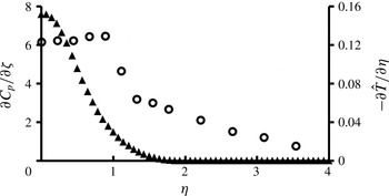
Axial accelerations within the flow field are affected by the local radial temperature gradient that provides a radial buoyancy force. Figure 7 shows the radial distribution the radial gradient of normalized temperature, $-\unicode[STIX]{x2202}\hat{T}/\unicode[STIX]{x2202}\unicode[STIX]{x1D702}$ . These data show that the temperature gradient has a local maximum near $\unicode[STIX]{x1D702}=1$ , drops sharply within $1<\unicode[STIX]{x1D702}<1.33$ to $0.5(-\unicode[STIX]{x2202}\hat{T}/\unicode[STIX]{x2202}\unicode[STIX]{x1D702})_{max}$ and thereafter decreases. However, within the vortex core, where $-\unicode[STIX]{x2202}\hat{T}/\unicode[STIX]{x2202}\unicode[STIX]{x1D702}$ is nearly invariant ( $\hat{T}$ decreases nearly linearly from $0<\unicode[STIX]{x1D702}<1$ , cf. figure 5 b), ${\hat{w}}$ decreases towards the centreline (cf. figure 5 a). As shown in (2.10), the radial distribution of axial momentum depends on both the local $\hat{T}(\unicode[STIX]{x1D702})$ (i.e. $g^{\prime }$ ) and the axial component of the gradient of the pressure coefficient, $\unicode[STIX]{x2202}C_{p}/\unicode[STIX]{x2202}\unicode[STIX]{x1D701}$ . The pressure within the vortex core is lowest near the surface where the tangential velocity has a maximum and increases in the vertical direction, leading to a downward force that reduces the effect of buoyancy and leads to the reduction in axial velocity along the axis of symmetry. The radial variation of the axial component of the gradient of the pressure coefficient (figure 7) is only non-zero when $\unicode[STIX]{x1D702}<1.5$ . These data indicate that the vertical pressure gradient along the centreline deflects the axial flow radially and thereby affects a local maximum of the axial velocity near $\unicode[STIX]{x1D702}\approx 1$ , in contrast to non-rotating, thermal plumes which typically have an axial velocity maximum along the vertical axis of symmetry. Therefore, while the axial momentum of the columnar vortex is affected by the radial distributions of both the radial temperature and axial pressure gradients (cf. § 2), each is dominant in a different radial domain.

Figure 7.

Radial variation of the normalized radial temperature gradient (○) and the axial component of the gradient of the pressure coefficient (▴).

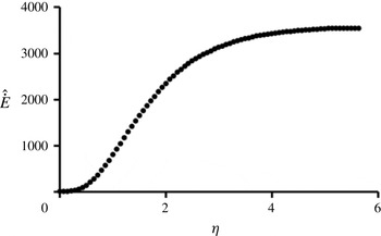
The axial velocity distribution, coupled with the angular momentum of the rotating vortex column, determine the magnitude and radial distribution of kinetic energy flux within the vortex core and the outer flow. The radial distribution of the integral of the kinetic energy flux ${\dot{E}}=2\unicode[STIX]{x03C0}\int _{0}^{r}(\unicode[STIX]{x1D70C}/2)(v^{2}+w^{2})(\boldsymbol{V}\cdot \hat{n})r^{\prime }\,\text{d}r^{\prime }$ through a radially expanding, circular surface of radius $r$ , centred about the $z$ axis at a fixed height $\unicode[STIX]{x1D701}=0.12$ and $\hat{{\dot{E}}}={\dot{E}}/(\unicode[STIX]{x1D70C}\unicode[STIX]{x1D708}gR^{2})$ is shown in figure 8. The contribution of the radial velocity component to the second factor in the integrand is neglected because $u$ is small compared to $v$ and $w$ (cf. figure 5). Within the inner domain of the vortex core, $\unicode[STIX]{x1D702}<0.5$ , the integral of the kinetic energy flux is negligible ( $\hat{{\dot{E}}}<0.04\hat{{\dot{E}}}_{max}$ ). Near $\unicode[STIX]{x1D702}=1$ , the integral of flux increases rapidly, and for $\unicode[STIX]{x1D702}>2$ , begins to level off, reaching a nominally invariant value near $\unicode[STIX]{x1D702}=4$ . At this distance from the vortex centreline, the magnitude of the axial velocity decreases (cf. figure 5 a), resulting in a reduction in the flux of energy through the control surface near the outer edge of the vane enclosure. The distribution of kinetic energy therefore implies that the majority of the energy within the vane enclosure is available within the outer flow domain of the vortex column ( $1<\unicode[STIX]{x1D702}<4$ ), i.e. outside the core itself ( $\unicode[STIX]{x1D702}<1$ ). Although the flow field maintains a considerable fluid torque outside of the annular domain ( $\unicode[STIX]{x1D702}>4$ ) due to the significant tangential velocity (cf. figure 5(a)) associated with the entrained flow, the small axial velocity at $\unicode[STIX]{x1D702}>4$ reduces the contributions of this angular momentum to ${\dot{E}}$ .

Figure 8.

Radial distribution of the normalized integrated kinetic energy flux through $\unicode[STIX]{x1D701}=0.12$ at varying circular control surface radii.

4.2 Axial similarity

The vertical evolution of the vortex core and surrounding outer flow is investigated by considering the axial similarity of the nominal vortex. As noted in § 2, in the absence of external flow boundaries, buoyancy-induced columnar vortices may be thought of as a ‘superposition’ of two self-similar flows (i.e. non-rotating, thermal plumes and momentum-driven, swirling jets) and, therefore, it is hypothesized that a free buoyant, columnar vortex may also be self-similar. This hypothesis is tested using the anchored vortex in the laboratory facility.

The flow field of the nominal anchored, columnar vortex is investigated using radial distributions of the time- and azimuthally averaged tangential and axial velocity components and temperature at ten equally spaced horizontal planes, 2.5 cm apart ( $\unicode[STIX]{x0394}z/h=0.042$ ), above the heated surface starting at $z=2.5$ cm ( $z/h=0.042$ ). Additional SPIV measurements are acquired in a vertical plane ( $r$ – $z$ ) at $\unicode[STIX]{x1D703}=0^{\circ }$ (corresponding to the azimuthal location between the enclosure centreline and a vane pivot, cf. figure 15(a)) above the heated surface ( $0.0015\leqslant z/h\leqslant 0.082$ , with resolution of $\unicode[STIX]{x0394}z/h=0.0015$ ), augmented by temperature measurements using a vertical array of thermocouple sensors (placed $\unicode[STIX]{x0394}z/h=0.005$ apart, cf. § 3). These data are recorded for a single $\unicode[STIX]{x1D703}$ -plane, and the time-averaged flow is assumed to be axisymmetric, which neglects the 12-fold symmetry of the enclosure. Following the analysis in § 2, the measured velocity field is used to extract the axial variation of each characteristic scale of the nominal vortex flow, the core radius $R(z)$ (defined by the radial location of the peak tangential velocity), centreline weight deficiency $g^{\prime }(0,z)\;[g^{\prime }=g(T-T_{\infty })/T_{\infty }]$ , and tangential and axial velocity components at $r=R$ , namely $v(R,z)$ and $w(R,z)$ respectively. The axial variations are plotted in figures 9(a) through (d) with respect to $z/h$ , a dimensionless geometric height normalized by the height of the array of azimuthal flow vanes ( $h=0.6$ m).

Figure 9.

Axial variations of the: ( $a$ ) vortex core radius, ( $b$ ) centreline weight deficiency, ( $c$ ) tangential velocity and ( $d$ ) axial velocity at $r=R$ ( $\unicode[STIX]{x1D702}=1$ ) for ( $Gr=9.7\times 10^{7}$ , $\unicode[STIX]{x1D711}=30^{\circ }$ ). The functional fit of each data set is shown using a dashed line (– –).

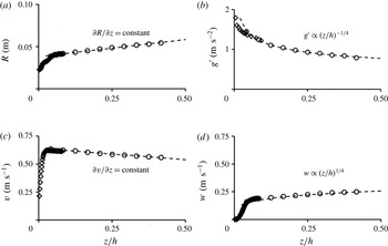
Figure 9(a) shows that for $z/h>0.038$ , the vortex core radius (defined by $R$ ) increases linearly with elevation, $\unicode[STIX]{x2202}R/\unicode[STIX]{x2202}z=0.056$ , as the vortex core spreads radially due to entrainment along the edge of the vortex core. The characteristic height, $\unicode[STIX]{x1D6FF}_{d}=z/h=0.038$ , denotes the top of the development region that includes the surface boundary layer (cf. figure 2) and the lowest extent of the nominal vortex column above which the flow can be described as self-similar. As discussed in § 2, the scaling of the continuity equation yields $R/z\propto (u_{e}/\bar{w})|_{r=R}$ . Therefore, along the ray $R=\unicode[STIX]{x1D6FC}z$ , $u/w=\unicode[STIX]{x1D6FC}$ and the entrainment coefficient of the nominal (base) vortex as defined by the slope of the dashed line in figure 9(a), is 0.056 which is lower than the entrainment coefficient of a corresponding thermal plume ( $\unicode[STIX]{x1D6FC}=O[0.1]$ , Turner Reference Turner1962). This difference may be attributed to enhanced exchange of mass and momentum within the outer flow region of the columnar vortex compared to a corresponding non-rotating, thermal plume. As a result of the diminished entrainment and mixing of cool ambient air into the core of the columnar vortex, the centreline weight deficiency (i.e. centreline air temperature) decreases at a lower rate, $g^{\prime }\propto z^{-1/4}$ (figure 9 b) compared to the axial rate of a non-rotating, thermal plume in an unstably stratified air layer over a horizontal heated surface ( $g^{\prime }\propto z^{-1/3}$ , Turner Reference Turner1969). Previous investigators (e.g. Kaimal & Busigner Reference Kaimal and Busigner1970) argued that for given thermal resources, the axial fluxes of mass and momentum within columnar vortices are at least an order of magnitude larger than the corresponding fluxes in nonrotating plumes. Therefore, since the entrainment coefficient of a round plume is larger than that of a columnar vortex, the bulk of the contribution to these fluxes must originate within the radially unbounded flow along the heated ground plane as alluded to by figure 9(b). This also indicates that while the concept of a virtual origin is appropriate for scaling of relevant axisymmetric shear flows that are characterized by conserved global momentum flux or heat flux (Morton et al. Reference Morton, Taylor and Turner1956; Hunt & Kaye Reference Hunt and Kaye2001), its applicability to a buoyancy-induced columnar vortex, in which the axial momentum flux increases with elevation as implied by (2.6), is questionable. Although the collapse of the radial distributions of the axial and tangential velocity components (cf. figure 11) indicates fixed axial momentum flux and azimuthal momentum, the distribution of the collapsed weight deficiency (cf. figure 11) does not vanish for large $r$ since the axisymmetric flow along the heated ground plane that ultimately converges into the vortex core is, in principle, radially unbounded. In fact, the present data (figure 9 b) indicate that the buoyancy flux through the columnar vortex is not conserved, $\unicode[STIX]{x2202}{\dot{B}}/\unicode[STIX]{x2202}z\neq 0$ , due to the stratified environment surrounding the vortex core within the enclosure volume ( $\unicode[STIX]{x2202}\unicode[STIX]{x1D70C}_{\infty }/\unicode[STIX]{x2202}z\neq 0$ for $r>R$ , Turner Reference Turner1973).

As shown in figure 9(c), the peak tangential velocity decreases linearly with elevation at a rate $\unicode[STIX]{x2202}[v(R)]/\unicode[STIX]{x2202}(z/h)=-0.2$ , similar to non-buoyant, swirling jets (e.g. Chigier & Chervinsky Reference Chigier and Chervinsky1967). However, in contrast to the decay of the axial velocity in similar non-buoyant, swirling flows ( $w\propto z^{-3/2}$ , Rajaratnam Reference Rajaratnam1976) the axial velocity in the buoyant, columnar vortex continues to accelerate well above the development region, $\unicode[STIX]{x1D6FF}_{d}$ , owing to the non-zero weight deficiency within its core. The vertical evolution of axial velocity at $r=R$ ( $\unicode[STIX]{x1D702}=1$ ) increases like $z^{1/4}$ , slower than a corresponding thermal plume formed from natural convection ( $w\propto z^{1/3}$ , Turner Reference Turner1969) ostensibly owing to the downward pressure force, that does not occur in non-rotating plumes and which counters the upward force of buoyancy within the vortex core (cf. § 4.1, figure 7).

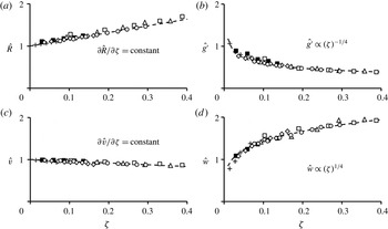
The axial similarity is extended to include a range of formation parameters (i.e. $Gr$ and $\unicode[STIX]{x1D711}$ ). Figure 10 shows the axial variation with the similarity coordinate $\unicode[STIX]{x1D701}$ ( $\unicode[STIX]{x1D6FC}z/R$ ) of the vortex core radius, centreline weight deficiency, tangential velocity and axial velocity measured at $r=R$ ( $\unicode[STIX]{x1D702}=$ 1). Each of these variables is normalized by its respective asymptotic characteristic scale $R_{0}$ , $v_{0}$ , $w_{0}$ and ${g^{\prime }}_{0}$ at $\unicode[STIX]{x1D701}=0.01$ (since $w_{0}$ and ${g^{\prime }}_{0}$ vanish at $\unicode[STIX]{x1D701}=0$ ). To demonstrate a broader range of the similarity, these data are acquired at $Gr=4.8$ , 9.7, and $11.6\times 10^{7}$ and $\unicode[STIX]{x1D711}=20^{\circ }$ and $30^{\circ }$ . These data clearly exhibit a collapse that is similar to figure 9. It is noted that the entrainment coefficient depends both on $Gr$ and $\unicode[STIX]{x1D711}$ and for the present data varies between 0.02 and 0.07. It was found that $\unicode[STIX]{x1D6FC}$ decreases monotonically with $Gr$ as the vortex entrains less fluid along its periphery (well above the ground plane) and the cross-stream spreading of its radius $R$ diminishes with increasing thermal forcing. Therefore, the normalized height of the measurement domain ( $0.042<z/h<0.42$ ) decreases and the magnitudes of the characteristic scales change less rapidly with increased $Gr$ . 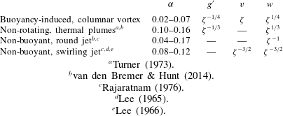The axial scaling of the primary parameters of the columnar vortex in figure 10 is compared with the scaling of a thermal plume, a round jet, and a swirling jet, in table 1.

Figure 10.

Axial variations within the similarity domain of ( $a$ ) vortex core radius, ( $b$ ) centreline weight deficiency, ( $c$ ) tangential velocity and ( $d$ ) axial velocity at $r=R$ ( $\unicode[STIX]{x1D702}=1$ ) measured at $\unicode[STIX]{x1D711}=20^{\circ }$ and $30^{\circ }$ for $Gr=4.8\times 10^{7}$ (▵, ▫), $9.7\times 10^{7}$ (♢, ○) and $11.6\times 10^{7}$ ( $+$ , ▪). The functional fit of each data set is shown using a dashed line (– –).

Table 1.

Comparison of the axial scaling of the primary parameters in figure 10 with a thermal plume, round jet and a swirling jet.

$^{a}$ Turner (Reference Turner1973).

$^{b}$ van den Bremer & Hunt (Reference van den Bremer and Hunt2014).

$^{c}$ Rajaratnam (Reference Rajaratnam1976).

$^{d}$ Lee (Reference Lee1965).

$^{e}$ Lee (Reference Lee1966).

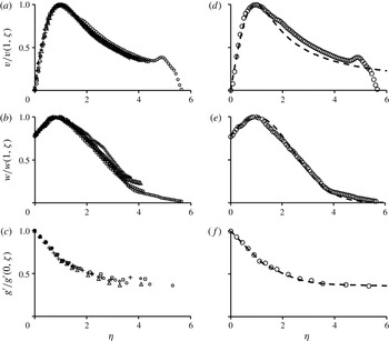
The similarity of the nominal vortex is further investigated by examining radial distributions within the vertical domain $0.042<z/h<0.42$ ( $2.5~\text{cm}<z<25~\text{cm}$ ). Figures 11(a–c) show radial distributions of time- and azimuthally averaged tangential and axial velocity components and weight deficiency in similarity coordinates [ $\unicode[STIX]{x1D702}=r/R(\unicode[STIX]{x1D701}),\unicode[STIX]{x1D701}=\unicode[STIX]{x1D6FC}z/R(\unicode[STIX]{x1D701})$ ] at five equally spaced axial elevations $\unicode[STIX]{x0394}z=$ 5 cm apart starting at $z=5$ cm ( $\unicode[STIX]{x1D701}\approx 0.07$ ). At each elevation, each velocity component is scaled by its value at $\unicode[STIX]{x1D702}=1$ and the weight deficiency is scaled by its value at $\unicode[STIX]{x1D702}=0$ . At $\unicode[STIX]{x1D701}=0.07$ , 0.17, 0.22 and 0.26 the radial extent of the measurement domain is $0<\unicode[STIX]{x1D702}<4.5$ , while at $\unicode[STIX]{x1D701}=0.12$ the radial domain extends past the inner edge of the vanes to $\unicode[STIX]{x1D702}=5.66$ . The collapse of these data indicates that, for the nominal, anchored vortex, the axial evolution of the core and surrounding outer flow is reasonably self-similar within $0<\unicode[STIX]{x1D702}<4.5$ , despite the length scale imposed by the array of vanes.

Figure 11.

Radial distributions of the time- and azimuthally averaged ( $a$ ) tangential and ( $b$ ) axial velocity components and ( $c$ ) weight deficiency at elevations $\unicode[STIX]{x1D701}=0.07$ (▫), 0.12 (○) 0.17 (▵), 0.22 (♢) and 0.26 ( $+$ ) normalized by their respective maxima at each elevation. Fitted variation to each measured distribution is shown on the right ( $d,e$ and $f$ ) using dashed lines (– –) along with the corresponding measured distribution at $\unicode[STIX]{x1D701}=0.12$ (○).

The radial distributions of tangential velocity in similarity coordinates (figure 11 a) imply that the linear variation of peak tangential velocity with $\unicode[STIX]{x1D701}$ at $\unicode[STIX]{x1D702}=1$ (cf. figure 9 c) holds for all $\unicode[STIX]{x1D702}$ within the domain $0<\unicode[STIX]{x1D702}<4.5$ . An approximate functional dependence for the radial distribution of tangential velocity, $h(\unicode[STIX]{x1D702})$ (cf. equation 2.8) is inspired by the tangential velocity of the Lamb–Oseen two-dimensional model of a viscous vortex, $v=\unicode[STIX]{x1D6E4}(1-\text{e}^{-(r/R)^{2}})/(2\unicode[STIX]{x03C0}r)$ . Using the axial circulation of the vortex column, computed from the measured radial distribution of tangential velocity, $\unicode[STIX]{x1D6E4}_{z}=2\unicode[STIX]{x03C0}\int -\unicode[STIX]{x2202}(rv)/\unicode[STIX]{x2202}r\,\text{d}r$ , the tangential velocity distribution in similarity coordinates is given by $v(\unicode[STIX]{x1D702},\unicode[STIX]{x1D701})=v(R,\unicode[STIX]{x1D701})h(\unicode[STIX]{x1D702})=\unicode[STIX]{x1D6E4}_{z}(\unicode[STIX]{x1D701})(1-\text{e}^{-\unicode[STIX]{x1D702}^{2}})/(2\unicode[STIX]{x03C0}\unicode[STIX]{x1D702}R(\unicode[STIX]{x1D701}))$ , plotted in figure 11(d) along with the data measured at $\unicode[STIX]{x1D701}=0.12$ . These data show reasonable agreement for $0\leqslant \unicode[STIX]{x1D702}\leqslant 1.75$ . Since the anchored, columnar vortex is radially confined by the vanes, the tangential velocity distribution does not vanish at large $\unicode[STIX]{x1D702}$ as is predicted by the Lamb–Oseen model. It is therefore conjectured that the slight mismatch between $h(\unicode[STIX]{x1D702})$ and the measured distributions within the annular domain $1.75<\unicode[STIX]{x1D702}<4.5$ , results from the azimuthal momentum contributed to the outer flow by the entrainment wall jet.

Unlike the tangential velocity, the radial distributions of the axial velocity (figure 11 b) exhibit some dispersion with increasing elevation for $\unicode[STIX]{x1D702}>2$ , ostensibly as a result of the variation of the entrainment through the vanes with elevation. The measured radial distributions are used to obtain a functional fit, $f(\unicode[STIX]{x1D702})$ (cf. equation 2.8), to describe $w(\unicode[STIX]{x1D702},\unicode[STIX]{x1D701})$ based on a Gaussian function, which is frequently used to approximate the time-averaged distribution of axial velocity in non-rotating thermal plumes and jets. Since the radial distribution of the axial velocity in the columnar vortex has a maximum away from the centreline (cf. figure 5), $f(\unicode[STIX]{x1D702})$ is a shifted Gaussian centred at $\unicode[STIX]{x1D702}=0.85$ and scaled by the radial location at which the magnitude of the normalized axial velocity, ${\hat{w}}$ is $\text{e}^{-1}$ of the peak value (i.e. $\unicode[STIX]{x1D702}\approx 3$ ). Using this description, the axial velocity in similarity coordinates is approximated by $w(\unicode[STIX]{x1D702},\unicode[STIX]{x1D701})=w(1,\unicode[STIX]{x1D701})f(\unicode[STIX]{x1D702})=w(1,\unicode[STIX]{x1D701})\text{e}^{-(\unicode[STIX]{x1D702}-1)^{2}/4}$ shown in figure 11(e) with the measured axial velocity at $\unicode[STIX]{x1D701}=0.12$ . Good agreement is obtained over the entire measurement domain ( $0<\unicode[STIX]{x1D702}<5.66$ ).

The weight deficiency of the columnar vortex is plotted in similarity coordinates in figure 11(c) and shows good collapse for each measurement plane. Similar to the distributions of tangential velocity, the presence of the vanes prevents $g^{\prime }$ from vanishing for large $\unicode[STIX]{x1D702}$ , because $T(\unicode[STIX]{x1D702}=5.44)>T_{\infty }$ at all elevations within the vane enclosure volume. Due to the form of the radial distribution of weight deficiency, it is necessary to divide the fit, $m(\unicode[STIX]{x1D702})$ (cf. equation 2.8), into two domains: the vortex core ( $\unicode[STIX]{x1D702}<1$ ) and outer flow ( $1<\unicode[STIX]{x1D702}$ ). Outside the vortex core, $\unicode[STIX]{x1D702}>1$ , the weight deficiency assumes a Gaussian distribution centred about $\unicode[STIX]{x1D702}=0,g^{\prime }(\unicode[STIX]{x1D702},\unicode[STIX]{x1D701})=g^{\prime }(0,\unicode[STIX]{x1D701})m(\unicode[STIX]{x1D702})=g^{\prime }(0,\unicode[STIX]{x1D701})[\unicode[STIX]{x1D6FE}\{1-g^{\prime }(5.44,\unicode[STIX]{x1D701})/g^{\prime }(0,\unicode[STIX]{x1D701})\}\text{e}^{-\unicode[STIX]{x1D702}^{2}/4}+g^{\prime }(5.44,\unicode[STIX]{x1D701})/g^{\prime }(0,\unicode[STIX]{x1D701})]$ scaled by a fraction, $\unicode[STIX]{x1D6FE}$ , of its centreline value and offset such that $g^{\prime }\rightarrow g^{\prime }(5.44,\unicode[STIX]{x1D701})$ at the radial edge of the vane enclosure. The measured temperatures within the vortex core show a linear increase of weight deficiency, described by $g^{\prime }(\unicode[STIX]{x1D702},\unicode[STIX]{x1D701})=g^{\prime }(0,\unicode[STIX]{x1D701})m(\unicode[STIX]{x1D702})=g^{\prime }(0,\unicode[STIX]{x1D701})[1+\unicode[STIX]{x1D702}(g^{\prime }(1,\unicode[STIX]{x1D701})/g^{\prime }(0,\unicode[STIX]{x1D701})-1)]$ for $\unicode[STIX]{x1D702}<1$ . The fit (figure 11 f) is in good agreement with the measured data for $\unicode[STIX]{x1D701}=0.12$ . Typically, for non-rotating thermal plumes, it is assumed that the radial distribution of weight deficiency has a Gaussian shape (Turner Reference Turner1969). Clearly, the weight deficiency of the nominal vortex deviates from this distribution when $\unicode[STIX]{x1D702}<1$ , displaying elevated temperatures within this domain compared to the inwardly extended Gaussian distribution used to describe the outer flow with $g^{\prime }(0,\unicode[STIX]{x1D701})_{Gaussian}/g^{\prime }(0,\unicode[STIX]{x1D701})_{actual}=\unicode[STIX]{x1D6FE}=0.6$ . Therefore, the nominal vortex displays a warmer core (cf. figure 9 b) than would be expected for a non-rotating plume formed under the same thermal conditions, again owing to the reduction of entrainment along the edge of the vortex core (cf. figure 9 a).

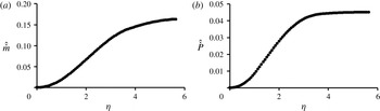
The radial distribution of the axial velocity at $\unicode[STIX]{x1D701}=0.12$ in figure 11(e) is used to compute the integrals of the axial mass and momentum fluxes through a circular surface of radius $r$ centred about the $z$ axis where ${\dot{m}}=\int _{0}^{2\unicode[STIX]{x03C0}}\int _{0}^{r}\unicode[STIX]{x1D70C}wr^{\prime }\,\text{d}r^{\prime }\,\text{d}\unicode[STIX]{x1D703}=2\unicode[STIX]{x03C0}\unicode[STIX]{x1D70C}w(1,\unicode[STIX]{x1D701})R^{2}\int _{0}^{\unicode[STIX]{x1D702}}f(\unicode[STIX]{x1D702}^{\prime })\unicode[STIX]{x1D702}^{\prime }\,\text{d}\unicode[STIX]{x1D702}^{\prime }$ and ${\dot{P}}=\int _{0}^{2\unicode[STIX]{x03C0}}\int _{0}^{r}\unicode[STIX]{x1D70C}w^{2}r^{\prime }\,\text{d}r^{\prime }\,\text{d}\unicode[STIX]{x1D703}=2\unicode[STIX]{x03C0}\unicode[STIX]{x1D70C}w(1,\unicode[STIX]{x1D701})^{2}R^{2}\int _{0}^{\unicode[STIX]{x1D702}}f(\unicode[STIX]{x1D702}^{\prime })^{2}\unicode[STIX]{x1D702}^{\prime }\,\text{d}\unicode[STIX]{x1D702}^{\prime }$ (figures 12 a,b). The integrals of the mass and axial momentum fluxes are each normalized by a reference flux $(\hat{{\dot{m}}}={\dot{m}}/{\dot{m}}_{ref},\hat{{\dot{P}}}={\dot{P}}/{\dot{P}}_{ref})$ based on a radially uniform distribution of the characteristic axial velocity $w=w(\unicode[STIX]{x1D702}=1,\unicode[STIX]{x1D701}=0.12)$ through the cross-section of the vortex core $(0<\unicode[STIX]{x1D702}<1)$ . While $\hat{{\dot{m}}}$ increases monotonically throughout the radial domain, $\hat{{\dot{P}}}$ increases linearly within the domain $1<\unicode[STIX]{x1D702}<3$ and saturates to $\hat{{\dot{P}}}=2.6$ at $\unicode[STIX]{x1D702}\approx 3.5$ , indicating an upper bound on the integral of the axial flux of linear axial momentum, resulting in the invariance of the integral of the kinetic energy flux for $\unicode[STIX]{x1D702}>4$ . From the expressions obtained in figure 10, the axial variation of the integrals of the mass and axial momentum fluxes can be written as $2\unicode[STIX]{x03C0}\unicode[STIX]{x1D70C}_{0}w(1,\unicode[STIX]{x1D701})R(\unicode[STIX]{x1D701})^{2}\unicode[STIX]{x1D701}^{9/4}$ and $2\unicode[STIX]{x03C0}\unicode[STIX]{x1D70C}_{0}w(R,\unicode[STIX]{x1D701})^{2}R(\unicode[STIX]{x1D701})^{2}\unicode[STIX]{x1D701}^{5/2}$ , respectively, in a form similar to the expressions derived by Batchelor (Reference Batchelor1954) and Turner (Reference Turner1973) for turbulent, non-rotating thermal plumes in an unstably stratified environment (for which ${\dot{m}}\propto \unicode[STIX]{x1D701}^{7/3}$ and ${\dot{P}}\propto \unicode[STIX]{x1D701}^{8/3}$ ). The present measurements show that the axial rate of increase of the integrals of the mass and axial momentum fluxes within the nominal vortex is smaller than the corresponding quantity in the thermal plume, consistent with the fact that the entrainment coefficient, $\unicode[STIX]{x1D6FC}$ , is smaller than that of a nominal non-rotating, thermal plume (cf. table 1). This result is evident in (2.10), which shows that the axial gradient of the axial momentum is diminished in the presence of a non-zero tangential velocity owing to the adverse axial pressure gradient imposed within the rotation of the core flow, which counteracts the buoyancy and ultimately leads to a reduction in the axial velocity along the axis of rotation.

Figure 12.

Radial variation of normalized integrals of the ( $a$ ) mass and ( $b$ ) axial momentum flux through $\unicode[STIX]{x1D701}=0.12$ at varying circular control surface radii ( $Gr=9.7\times 10^{7}$ , $\unicode[STIX]{x1D711}=30^{\circ }$ ).

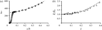
The axial variation of the normalized integral of the kinetic energy flux, $\hat{\dot{E}}={\dot{E}}/[\unicode[STIX]{x1D70C}\unicode[STIX]{x1D708}g(4R)^{2}]$ , is shown in figure 13(a) ( $Gr=9.7\times 10^{7}$ , $\unicode[STIX]{x1D711}=30^{\circ }$ ). These data are integrated across a horizontal cross-section of radius $\unicode[STIX]{x1D702}=4$ that corresponds to the radial location at which $\hat{\dot{E}}$ saturates with $\unicode[STIX]{x1D702}$ (cf. figure 8). The flux is computed at ten equally spaced axial elevations ( $0.042<z/h<0.42$ ) and augmented with SPIV measurements within the $r$ – $z$ plane ( $0<z/h<0.08$ ). These data show two distinct axial domains. Close to the surface, within $0\leqslant z/h\leqslant 0.04$ , $\hat{{\dot{E}}}$ increases rapidly from 0 to approximately 300. This sharp rise occurs as flow near the surface is turned vertically near the central stagnation point, resulting in significantly larger axial velocities than can be induced by buoyancy alone. In the second domain ( $0.04\leqslant z/h\leqslant 0.42$ ), the axial rate of change of the integral of the kinetic energy flux diminishes considerably, and the axial acceleration is dominated by buoyancy. Within this domain, the available extractable power increases nearly 2-fold [ $\hat{{\dot{E}}}(z/h=0.05)=1.9\hat{{\dot{E}}}(z/h=0.42)$ ] and varies as $(z/h)^{2}$ . The increase in the integral of the kinetic energy flux with elevation continues as long as the axial velocity accelerates due to buoyancy [cf. (2.10)]. While the rotation-induced, axially adverse pressure gradient within the core of the vortex somewhat mutes the effect of the buoyancy force and, therefore, the axial rate of increase in axial momentum flux, this pressure gradient is far weaker within the outer flow. The axial and azimuthal flows within this outer annular domain include the majority of the kinetic energy (cf. figure 8) and are driven by the motions of the inner core flow and the entrainment through the vanes. This axial and azimuthal flow generates significantly more power than could be produced by natural convection alone. The similarity variation of the integral of the kinetic energy flux is extended over a range of formation parameters $Gr=4.8$ , 9.7 and $11.6\times 10^{7}$ and $\unicode[STIX]{x1D711}=20^{\circ }$ and $30^{\circ }$ as shown in figure 13(b) scaling the axial coordinate as $\unicode[STIX]{x1D701}(\unicode[STIX]{x1D6FC}z/R)$ (cf. figure 10 a) and normalizing $\hat{\dot{E}}$ by the respective asymptotic characteristic scale ${\dot{E}}_{0}$ , as $\unicode[STIX]{x1D701}\rightarrow 0$ . As shown in figure 13(b), these data show that the similarity of the base flow extends over a broad range of formation parameters and the extractable power varies as $\unicode[STIX]{x1D701}^{2}$ . The magnitude of increase of the integral of the kinetic energy flux, ${\dot{E}}_{0}$ , decreases with $Gr$ (cf. figure 10) and, therefore, the majority of increase is primarily attributed to the entrainment of heated flow along the ground plane.

Figure 13.

( $a$ ) Variation of the normalized integral of kinetic energy flux with elevation ( $Gr=9.7\times 10^{7}$ , $\unicode[STIX]{x1D711}=30^{\circ }$ ) and ( $b$ ) axial variations of the normalized integral of kinetic energy flux at $\unicode[STIX]{x1D711}=20^{\circ }$ for $Gr=4.8$ (▵), 9.7 (♢) and $11.6\times 10^{7}$ ( $+$ ) and $\unicode[STIX]{x1D711}=30^{\circ }$ for $Gr=4.8$ (▫), 9.7 (○) and $11.6\times 10^{7}$ (▪).

As shown in (2.10), the axial momentum equation in similarity variables depends on two (dimensionless) parameters at each elevation $\unicode[STIX]{x1D701}=Z$ , namely, the swirl number and Froude number [ $S(Z)=v(1,Z)/w(1,\text{Z})$ , and $Fr(Z)=([\unicode[STIX]{x1D6FC}w^{2}(1,Z)]/[2g^{\prime }R(Z)])^{1/2}$ ]. The axial variations of $S(\unicode[STIX]{x1D701})$ and $Fr(\unicode[STIX]{x1D701})$ within the domain $0.036<\unicode[STIX]{x1D701}<0.26$ (in which the vortex is self-similar, cf. figure 9) are shown in figure 14. These data show that $S(\unicode[STIX]{x1D701})$ , which measures the vertical pitch of the helical motion at the edge of the vortex core and scales the axial pressure gradient term in the axial momentum equation [cf. (2.10)], decreases with elevation owing to the increase in axial velocity, $w\propto \unicode[STIX]{x1D701}^{1/4}$ (cf. figure 10(d) accompanied by a decrease in the tangential velocity (cf. figure 10 c). The rate of decrease of $S(\unicode[STIX]{x1D701})$ diminishes with elevation, and $S$ decays to less than 2 within the measurement domain. Concomitantly, $Fr$ , which measures the ratio of axial kinetic to buoyant potential energy, increases from 0.18 to 0.3 between $\unicode[STIX]{x1D701}=0.036$ and 0.26 as thermal energy is continually converted into mechanical (kinetic) energy. As noted in connection with the axial momentum (2.10), the dimensionless buoyant forcing term $\int _{0}^{\infty }m(\unicode[STIX]{x1D702})\unicode[STIX]{x1D702}\,\text{d}\unicode[STIX]{x1D702}$ is scaled by $Fr^{-2}$ , and so long as $Fr<1$ , the effect of the buoyancy is amplified. The Froude number increases with elevation, due to the decrease in weight deficiency in the vortex core, entrainment of cooler air along its vertical edge and a net increase in the axial velocity, in turn due to buoyancy-induced axial accelerations (as long as $g^{\prime }>0$ ). Therefore, the effect of buoyancy in (2.10) diminishes with elevation as the vortex core continues to cool. Eventually $g^{\prime }(0,\unicode[STIX]{x1D701})\rightarrow 0$ , $Fr\rightarrow \infty$ , and the flow is well approximated by a non-buoyant, swirling jet.

Figure 14.

Axial variation of ( $a$ ) Swirl ( $S$ ) and ( $b$ ) Froude ( $Fr$ ) numbers ( $Gr=9.7\times 10^{7}$ , $\unicode[STIX]{x1D711}=30^{\circ }$ ).

The radial distributions of local $S(\unicode[STIX]{x1D702})$ and $Fr(\unicode[STIX]{x1D702})$ are shown in figures 15(a) and 15(b), respectively, for $\unicode[STIX]{x1D701}=0.12$ , and are divided into three annular regimes based on the magnitude of the swirl number. While $S(\unicode[STIX]{x1D702})$ is computed directly from the velocity (SPIV) data (for which $\unicode[STIX]{x0394}\unicode[STIX]{x1D702}\approx 0.07$ ), the radial variation of $Fr(\unicode[STIX]{x1D702})$ is calculated at the location of each radial temperature measurement ( $\unicode[STIX]{x0394}\unicode[STIX]{x1D702}\approx 0.22$ for $\unicode[STIX]{x1D702}<1.76$ and $\unicode[STIX]{x0394}\unicode[STIX]{x1D702}=0.44$ for $\unicode[STIX]{x1D702}>1.76$ ). Region I ( $\unicode[STIX]{x1D702}<0.5$ ) is the inner vortex core in which $v$ increases faster than $w$ and $S$ increases nearly linearly. Within this domain, the weight deficiency and $Fr$ have a local maximum and minimum, respectively, along the centreline. Within Region II ( $0.5<\unicode[STIX]{x1D702}<3$ ) $S$ is nearly invariant through the edge of the core (at $\unicode[STIX]{x1D702}=1$ ), in the transition domain ( $1<\unicode[STIX]{x1D702}<1.8$ ) [cf. figure 5 a], and well into the outer flow. The vertical pitch of the helically swirling flow is nearly invariant over a wide range of $\unicode[STIX]{x1D702}$ . On the other hand, $Fr$ has a local maximum at $\unicode[STIX]{x1D702}=1$ (where $Fr=0.21$ ) and thereafter decreases nearly linearly to 0.09 at $\unicode[STIX]{x1D702}=3$ . Region III ( $\unicode[STIX]{x1D702}>3$ ) is characterized by the effects of the entrained flow, which leads to a radial increase in the tangential velocity, while $w(\unicode[STIX]{x1D702})$ decreases monotonically (cf. figure 5 a). As a result, $S$ increases sharply and has a peak of 20.5 at $\unicode[STIX]{x1D702}=4.9$ . $Fr$ continues to decrease with the axial velocity even as the weight deficiency remains nearly invariant with $\unicode[STIX]{x1D702}$ .

Figure 15.

Radial variation of ( $a$ ) Swirl ( $S$ ) and ( $b$ ) Froude ( $Fr$ ) numbers ( $\unicode[STIX]{x1D701}=0.12$ , $Gr=9.7\times 10^{7}$ , $\unicode[STIX]{x1D711}=30^{\circ }$ ).

5 The near-surface vortex structure

The mechanisms that drive the formation and sustainment of the vortex core and its outer flow take place within a relatively thin [ $z/h\approx O(0.017)$ ] swirling boundary layer over the heated surface. It is the interaction of this boundary layer with the induced buoyant instability and near-surface pressure forces that is responsible for the conversion of the thermal energy from the heated surface to the kinetic energy associated with the vortical flow. The conversion mechanism that generates and sustains the buoyancy-induced columnar vortex is associated with the production, and eventual tilting, of the induced horizontal vorticity concentrations within the ground-plane boundary layer.

5.1 The flow field near the ground plane

The thermal energy and vorticity concentrations that affect the structure and dynamics of the columnar vortex originate from the ground-plane boundary layer of entrained air over the heated surface. For $\unicode[STIX]{x1D711}=30^{\circ }$ and $Gr=9.7\times 10^{7}$ , the time-averaged flow field in an azimuthal plane passing through the centreline of the columnar vortex ( $\unicode[STIX]{x1D702}=0$ ) and the pivot location of an azimuthal vane and extending to the ground plane (figure 16 a) is shown in figure 16(b) using vectors of radial and axial velocity overlaid on a raster plot of the normalized tangential velocity, $\hat{v}$ , distribution. A raster plot of the corresponding normalized radial velocity, $\hat{u}$ , and normalized temperature distribution, $(T-T_{\infty })/(T_{p}-T_{\infty })$ , are shown in figures 16(c,d), respectively. These data are not azimuthally averaged and the flow field is assumed to be axisymmetric despite the 12-fold symmetry of the vane enclosure. These SPIV measurements are taken in four segments, assembled to form the investigation domain $0<r<18$ cm, $0<z<5$ cm. The data are normalized and similarity variables are defined using the core radius (4.5 cm) and angular velocity ( $15~\text{s}^{-1}$ ) of the vortex core at $z=10$ cm ( $\unicode[STIX]{x1D701}=0.12$ ) so that the interrogation domain in similarity coordinates is $0<\unicode[STIX]{x1D702}<4$ , $0<\unicode[STIX]{x1D701}<0.06$ and can readily be compared to the radial distributions of figure 5. Temperature measurements are recorded at $\unicode[STIX]{x0394}r=1$ cm ( $\unicode[STIX]{x0394}\unicode[STIX]{x1D702}=0.22$ ) increments using the vertical thermocouple rake over the identical radial plane ( $0<r<18$ cm, $0<z<5$ cm; $0<\unicode[STIX]{x1D702}<4$ , $0<\unicode[STIX]{x1D701}<0.06$ ). The velocity distributions elucidate several distinguishing characteristics of the single-cell vortex flow near the surface. As the flow near the edge of the measurement domain is entrained towards the centreline within the ground-plane boundary layer, the radial velocity at the top edge of the boundary layer ( $\unicode[STIX]{x1D6FF}=10.1$ mm at $\unicode[STIX]{x1D702}=4$ ), increases and develops a local maximum (e.g. $\unicode[STIX]{x1D6FF}=8.26$ mm at $\unicode[STIX]{x1D702}=2$ ) that monotonically increases and moves closer to the surface as $\unicode[STIX]{x1D702}$ decreases (see also figure 17). Simultaneously, the axial velocity component begins to increase at higher elevations, and closer to the centreline. Figure 16(d) shows that for a given elevation above the surface the temperature of the entrained air increases with decreasing $\unicode[STIX]{x1D702}$ , and, thereby, the effect of buoyancy is intensified and contributes to the increase in the magnitude of the axial velocity with elevation (cf. figure 9 d).

Figure 16.

( $a$ ) Side and top view of $\unicode[STIX]{x1D702}$ – $\unicode[STIX]{x1D701}$ measurement plane highlighted in green to denote the location of the laser sheet, and colour raster plots of ( $b$ ) normalized tangential velocity distributions superposed with vertical distributions of the in-plane velocity vectors, ( $c$ ) normalized radial velocity distributions and ( $d$ ) normalized temperature distribution in the $\unicode[STIX]{x1D702}$ – $\unicode[STIX]{x1D701}$ plane ( $Gr=9.7\times 10^{7}$ , $\unicode[STIX]{x1D711}=30^{\circ }$ ).

Figure 17.

Axial distributions of normalized radial velocity above the surface at $\unicode[STIX]{x1D702}=1$ , 2, 3 and 4 (○). The dashed line (– –) marks the location and trajectory of the maximum radial velocity at each radial station.

As the entrained flow near the ground plane approaches the centreline, it is turned upward and accelerated axially, forming a central stagnation point on the surface beneath the vortex column at $\unicode[STIX]{x1D702}=0$ , $\unicode[STIX]{x1D701}=0$ . This process is accompanied by a significant thickening of the thermal layer ( $\unicode[STIX]{x1D702}<1$ , figure 16 d) as the axial velocity leads to vertical advection of surface heated air into the vortex core. The upward turning of the flow is accompanied by a change in direction (and sign) of radial velocity, marked by the contour $u=0$ (white) in figure 16(c). The turning flow contracts at $\unicode[STIX]{x1D701}=0.02$ ( $z/h=0.027$ ) and the narrowest radial extent of its edge, defined by the maximum tangential velocity located at $\unicode[STIX]{x1D702}=0.67$ and referred to as a ‘vortex jump’ by Mullen & Maxworthy (Reference Mullen and Maxworthy1977), is discussed further in connection with figure 19. Following this contraction, the flow expands rapidly (as is evident by the increase of the domain in which $u>0$ ), and ultimately reaches a nominally invariant (self-similar) core radius at higher elevations, as discussed in § 4.2. Below $\unicode[STIX]{x1D701}<0.03$ ( $z/h<0.04$ ) a clear division between the domains containing $u>0$ and $u<0$ is identified. Above this elevation, negligible radial velocity is recorded in an increasingly larger radial band as the location of zero entrainment moves radially outwards towards $\unicode[STIX]{x1D702}=1.8$ at $\unicode[STIX]{x1D701}=0.12$ (cf. figure 5 a). As also shown in figure 16(b), the tangential velocity intensifies, reaches a maximum velocity at the location of the vortex contraction ( $\unicode[STIX]{x1D702}=0.67$ , $\unicode[STIX]{x1D701}=0.02$ ), and then migrates radially outward as the elevation increases, from $\unicode[STIX]{x1D702}=0.77$ at $\unicode[STIX]{x1D701}=0.03$ to $\unicode[STIX]{x1D702}=0.85$ at $\unicode[STIX]{x1D701}=0.06$ . For $\unicode[STIX]{x1D701}>0.03$ , the radial location of $v_{max}$ and the rate of spreading of the vortex core are determined by the entrainment coefficient, $\unicode[STIX]{x1D6FC}$ .

The evolution of the flow near the surface is shown in axial distributions of the radial velocity at $\unicode[STIX]{x1D702}=1$ , 2, 3 and 4 (figure 17). As the flow is entrained towards the base of the vortex column, the velocity distribution of the radial boundary layer evolves from a typical viscous layer (at $\unicode[STIX]{x1D702}=4$ ) into a distribution reminiscent of a wall jet (at $\unicode[STIX]{x1D702}=1$ ), as a result of the vortex-induced radial pressure gradient. As noted in § 4.1, the upper vortex column is in cyclostrophic balance (i.e. $\unicode[STIX]{x1D70C}v^{2}/r=\unicode[STIX]{x2202}p/\unicode[STIX]{x2202}r$ ). However, within the boundary layer, this force balance is modified by viscous effects at the heated surface, which slow the overlying flow, thus reducing the centripetal force and resulting in a net radial inward force due to the radial pressure gradient. As is evident in figure 17, the wall-jet flow near the surface couples the surface boundary layer and the overlying entrainment-driven flow (e.g. Wilson & Rotunno Reference Wilson and Rotunno1982) above and below the velocity peak that are each characterized by a layer of vorticity concentration of opposite sign (cf. figure 19). Baker (Reference Baker1981) showed experimentally that the combined thickness of the two vorticity layers should remain nominally invariant, while the height of the viscous layer becomes progressively smaller as the flow is entrained toward the vortex centreline. This observation is confirmed by the current measurements and denoted by the dashed line in figure 17. It is noteworthy that while the flow within the boundary layer accelerates with decreasing $\unicode[STIX]{x1D702}$ , the magnitude of the radial velocity above the boundary layer decreases as the flow approaches the centreline and is turned upward by the vertical motions of the vortex core, eventually changing signs for $\unicode[STIX]{x1D701}>0.03$ at $\unicode[STIX]{x1D702}\approx 0.8$ (cf. figure 16 b,c).

Assuming axisymmetry (i.e. disregarding the non-axisymmetric effects of the 12 vanes), the time-averaged data in the $r$ – $z$ plane shown in figure 16 are azimuthally swept to produce a three-dimensional volume that includes the swirling boundary layer and the bottom edge of the vertical vortex column. Streamlines are calculated from the time-averaged data by numerically releasing particles near the edge of the measurement domain within the boundary layer to obtain particle path lines of the steady flow field, and are displayed in an isometric view of the cylindrical domain $0<h<4$ and $0<z<0.06$ (figure 18) where the plane $z=0$ is a surface streamline. In the boundary layer, far from the vortex centreline, the radial and tangential velocities are comparable in magnitude and the entrained air spirals inward. The strength and direction of the swirling flow are determined by a balance between the angle set by the azimuthal flow vanes and the strength of the vortex-induced radial pressure gradient. As the flow approaches the centreline, the radial velocity increases and concentrates the flow at the base of the column, where it ultimately turns upward at the surface stagnation point and is accelerated by buoyancy. Once the flow is turned upwards, the streamlines that extend into the vortex column initially contract inwards before expanding radially and forming a helical pattern throughout the remainder of the vortex core.

Figure 18.

Three-dimensional path lines in the axisymmetric flow field showing the near-surface flow evolving into the columnar vortex located at the centre of the cylindrical domain created by the array of vanes.

Figure 19.

Colour raster plots of normalized vorticity concentrations in the $\unicode[STIX]{x1D702}$ – $\unicode[STIX]{x1D701}$ plane overlaid with in-plane velocity vectors: ( $a$ ) radial, ( $b$ ) azimuthal and ( $c$ ) axial ( $Gr=9.7\times 10^{7}$ , $\unicode[STIX]{x1D711}=30^{\circ }$ ).

5.2 Vorticity production mechanism

Buoyancy-induced, columnar vortices contain significant amounts of kinetic energy compared to nonrotating thermal plumes formed under the same conditions, due to the advection, tilting and stretching of the boundary layer vorticity. The axial turning of the surface flow near the centreline of the vortex is affected by the radial pressure gradient which, in turn, is affected by the angular momentum of the flow. Because the angular momentum is ultimately affected by the axial vorticity, it is instructive to examine the source of the vorticity within the vortex core. Contour plots of the three components of the time-averaged vorticity vector, $\unicode[STIX]{x1D74E}=(\unicode[STIX]{x1D714}_{r},\unicode[STIX]{x1D714}_{\unicode[STIX]{x1D703}},\unicode[STIX]{x1D714}_{z})=[-\unicode[STIX]{x2202}v/\unicode[STIX]{x2202}z,\unicode[STIX]{x2202}u/\unicode[STIX]{x2202}z-\unicode[STIX]{x2202}w/\unicode[STIX]{x2202}r,r^{-1}\unicode[STIX]{x2202}(rv)/\unicode[STIX]{x2202}r]$ , within the domain shown in figure 16(a), normalized by the angular velocity of the vortex core at $z/h=0.17$ ( $\unicode[STIX]{x1D6FA}=15~\text{s}^{-1}$ ) and calculated by assuming that azimuthal variation in the time-averaged data is negligible, are shown as $\hat{\unicode[STIX]{x1D714}}_{r}$ , $\hat{\unicode[STIX]{x1D714}}_{\unicode[STIX]{x1D703}}$ , and $\hat{\unicode[STIX]{x1D714}}_{z}$ in figures 19(a) through (c), respectively, overlaid with vectors of radial and axial velocity. The radial component of vorticity (figure 19 a) is positive throughout the boundary layer (the sign of the radial vorticity depends on the direction of rotation induced by the azimuthal flow vanes). These data show that radial vorticity is primarily concentrated within the surface layer, indicating that the axial variation of tangential velocity is comparatively small elsewhere (cf. figure 9 c). The radial vorticity has a local maximum at $\unicode[STIX]{x1D702}\approx 0.50$ and $0<\unicode[STIX]{x1D701}<0.01$ , beneath the vortex contraction (located at $\unicode[STIX]{x1D701}=0.02$ [ $z/h=0.027$ ]) where the tangential velocity is largest. The azimuthal vorticity (figure 19 b) exhibits the two layers of opposite sign associated with a wall-jet flow structure (cf. figure 17). Radial variations in the axial velocity within the contraction region of the forming vortex core contribute to the concentration of positive azimuthal vorticity layer along the periphery of the vortex core. The onset of the core of the columnar vortex can be inferred from axial vorticity concentrations (figure 19 c). These data show that the largest concentration of axial vorticity is confined to the domain $\unicode[STIX]{x1D702}<1$ . Within the columnar vortex, the peak axial vorticity occurs at the height of the vortex contraction along the vortex centreline ( $\unicode[STIX]{x1D702}=0$ , $\unicode[STIX]{x1D701}=0.02$ ) corresponding to the elevation where the angular velocity attains a maximum. For the current clockwise (from above) columnar vortex, the axial vorticity is negative.

The measured vorticity components are used to compute vortex lines (parallel to the vorticity vector at each point). Several vortex lines, originating within the near-wall region of the radial boundary layer, are shown in figure 20 along with vertical slices of axial vorticity at $\unicode[STIX]{x1D703}=0$ , $\unicode[STIX]{x03C0}/2$ , $\unicode[STIX]{x03C0}$ and $3\unicode[STIX]{x03C0}/2$ . The vortex core is distinguished by axial vorticity centred at $\unicode[STIX]{x1D702}=0$ , and can be considered as a concentration of vortex filaments stretched vertically. Within the viscous section of the radial boundary layer, the vortex lines form horizontal clockwise spirals, similar to the path lines shown in figure 18. The directional agreement between the vortex and streamlines does not occur for a vortex undergoing counter-clockwise (cyclonic) rotation, as the inward radial entrainment generates negative azimuthal vorticity within the viscous boundary layer regardless of the direction of the vortex rotation. In contrast, in a non-rotating thermal plume, the vortex lines within the boundary layer of the radially entrained flow form azimuthaly closed circles (or rings) centred around $\unicode[STIX]{x1D702}=0$ . These rings of azimuthal vorticity are compressed as they advect radially inward, before they are transported vertically by the axial flow. The swirling flow induced by the azimuthal flow vanes prevents the formation of closed, circular vortex rings around the axis of symmetry and allows for the spiraling vortex lines to be tilted axially. These vortex lines spiral inward at a nominally invariant pitch until reaching the domain directly beneath the core of the columnar vortex, where they are tilted. Once inside the vortex core, the helical (axial and azimuthal) vortex lines are stretched by axial gradients of vertical velocity. Note that, owing to the sign of the two layers of azimuthal vorticity, vortex lines that originate from within the positive azimuthal vorticity layer (above the local peak in the radial velocity component, cf. figures 16 c and 17) lead to vortex lines that spiral in an opposite direction than those shown in figure 20, and are ultimately tilted vertically outside the core ( $\unicode[STIX]{x1D702}>1$ ) of the vortex.

Figure 20.

Calculated vortex lines originating within the radial viscous boundary layer and tilted into the axial direction with contours of normalized axial vorticity denoting the location of the vortex core.

The tilting of horizontal vortex lines into the vertical direction is a result of the large gradients in velocity accompanying the vortex contraction. The axial vorticity transport equation shows that radial vorticity can be tilted in the vertical direction by radial gradients in the axial velocity: $\unicode[STIX]{x1D714}_{r}(\unicode[STIX]{x2202}w/\unicode[STIX]{x2202}r)$ . This term is computed from the SPIV data, normalized by the square of the angular velocity of the vortex core $\unicode[STIX]{x1D6FA}^{2}$ at $z/h=0.17$ , and displayed using a colour raster plot in figure 21(a). This figure also shows overlaid contour lines of the axial component of the vorticity vector (with an increment of $\unicode[STIX]{x0394}\unicode[STIX]{x1D714}_{z}/\unicode[STIX]{x1D6FA}=-1$ , starting at $\unicode[STIX]{x1D714}_{z}/\unicode[STIX]{x1D6FA}=-3$ ). These data show that the magnitude of the tilting term is significant within the domain directly below the vortex core ( $\unicode[STIX]{x1D702}<1$ , $\unicode[STIX]{x1D701}<0.02$ ), where the horizontal vortex lines are tilted into the axial direction in figure 20, and confirm that the interaction between the radial vorticity and radial gradient of axial velocity converts horizontal vorticity within the ground-plane boundary layer into axial vorticity within the core of the columnar vortex. It is also evident that additional tilting occurs above the location of the vortex contraction. At this location, a concentration of negative radial vorticity, centred about $\unicode[STIX]{x1D702}=0.2$ and $\unicode[STIX]{x1D701}=0.025$ (cf. figure 19 a), is generated due to the rapid radial expansion of the vortex column, and produces large axial gradients in tangential velocity ( $\unicode[STIX]{x1D714}_{r}=-\unicode[STIX]{x2202}v/\unicode[STIX]{x2202}z$ ). This additional tilting is visible in figure 20, where the vortex lines, once tilted axially, are directed radially outward above the vortex contraction before becoming nominally two-dimensional (axial and azimuthal) and forming a helical pattern in the remainder of the vortex column ( $\unicode[STIX]{x1D701}>0.03$ ; $z/h>0.044$ ). The axial circulation is computed from the radial distribution of tangential velocity as $\unicode[STIX]{x1D6E4}_{z}=2\unicode[STIX]{x03C0}\int -\unicode[STIX]{x2202}(rv)/\unicode[STIX]{x2202}r\text{d}r=-2\unicode[STIX]{x03C0}\unicode[STIX]{x1D6FA}R^{2}\int \unicode[STIX]{x2202}(\unicode[STIX]{x1D702}\hat{v})/\unicode[STIX]{x2202}\unicode[STIX]{x1D702}\text{d}\unicode[STIX]{x1D702}$ , (assuming axisymmetry) and is shown in figure 21(b). The contours clearly depict the tilting of the near-surface, horizontal vorticity within the viscous boundary layer into the vortex core. In fact, a given contour indicates the transition from low to high aspect ratio (axial to radial) cylindrical domains that bound the horizontal vorticity concentrations within the surface boundary layer and the axial vorticity concentrations within the core of the vortex. This is indicative of the change from the cross-stream scale of the boundary layer to the scale of the core of the vortex ( $z/r=0.23$ for $\unicode[STIX]{x1D6E4}_{z}/(2\unicode[STIX]{x03C0}\unicode[STIX]{x1D6FA}R^{2})=1$ ).

Figure 21.

( $a$ ) Colour raster plot of the normalized radial vorticity tilting term in the axial vorticity transport equation, overlaid with line contours of the axial vorticity and ( $b$ ) line contours of normalized axial circulation.

Since only the radial vorticity component contributes to the formation of axial vorticity within the core of the columnar vortex (the azimuthal vorticity does not change direction while it is advected into the vortex core), the radial circulation, $\unicode[STIX]{x1D6E4}_{r}$ , through the cross-section of a vortex tube within the surface boundary layer, should equal the axial circulation, $\unicode[STIX]{x1D6E4}_{z}$ , along the same variable-radius streamtube within the vortex core. For an axisymmetric flow,

(5.1)

$$\begin{eqnarray}\displaystyle \unicode[STIX]{x1D6E4}_{r}=\iint \unicode[STIX]{x1D714}_{r}r\,\text{d}\unicode[STIX]{x1D703}\,\text{d}z=-\mathop{\oint }_{2\unicode[STIX]{x03C0}}^{0}vr\,\text{d}\unicode[STIX]{x1D703}=2\unicode[STIX]{x03C0}rv=2\unicode[STIX]{x03C0}\unicode[STIX]{x1D6FA}R^{2}\unicode[STIX]{x1D702}\hat{v} & & \displaystyle\end{eqnarray}$$

and

(5.2)

$$\begin{eqnarray}\displaystyle \unicode[STIX]{x1D6E4}_{z}=\iint \unicode[STIX]{x1D714}_{z}r\,\text{d}\unicode[STIX]{x1D703}\,\text{d}r=\mathop{\oint }_{0}^{2\unicode[STIX]{x03C0}}vr\,\text{d}\unicode[STIX]{x1D703}=2\unicode[STIX]{x03C0}rv=2\unicode[STIX]{x03C0}\unicode[STIX]{x1D6FA}R^{2}\unicode[STIX]{x1D702}\hat{v}. & & \displaystyle\end{eqnarray}$$

The integrals of the radial and axial vorticity components are computed over the circumferential and top surfaces of a cylindrical control volume, respectively, of variable radius $0<r<18$ cm ( $0<\unicode[STIX]{x1D702}<4$ ) and a fixed height $0<z<5$ cm ( $0<\unicode[STIX]{x1D701}<0.06$ ). As shown in figure 22, the radial distributions of the normalized radial and axial circulations are nearly identical, demonstrating that the flux of radial vorticity into the columnar vortex is the sole source of the axial vorticity within the vortex core. Therefore, the contours of constant $\unicode[STIX]{x1D6E4}_{z}$ in figure 21(b) bound axisymmetric cylindrical bundles of vortex lines that bound the vertical core and the momentum boundary layer. Hence, the strength of the columnar vortex is completely determined by the production and tilting of the radial vorticity due to the azimuthal flow within the swirling ground-plane boundary layer.

Figure 22.

Comparison of normalized radial (●) and axial circulation (○) at varying cylindrical control surface radii.

Radial distributions of normalized axial ( $\hat{\unicode[STIX]{x1D714}}_{z}$ ) and azimuthal ( $\hat{\unicode[STIX]{x1D714}}_{\unicode[STIX]{x1D703}}$ ) vorticity components within the developed vortex column are computed at $\unicode[STIX]{x1D701}=0.12$ in the baseline vortex $\unicode[STIX]{x1D711}=30^{\circ }$ and $Gr=9.7\times 10^{7}$ ) and shown in figure 23. Within the inner core of the vortex, the axial vorticity rapidly decreases from its maximum along the centreline to $0.2\hat{\unicode[STIX]{x1D714}}_{z,max}$ at $\unicode[STIX]{x1D702}=1$ . Outside the vortex core, the magnitude of the axial vorticity continues to decrease before vanishing completely at $\unicode[STIX]{x1D702}=2$ , corresponding to the location where the radial distribution of tangential velocity resembles a potential vortex. Within the vortex column, the azimuthal vorticity, $(\unicode[STIX]{x2202}u/\unicode[STIX]{x2202}z)-(\unicode[STIX]{x2202}w/\unicode[STIX]{x2202}r)$ , is dominated by the radial gradient of axial velocity. It is negative within the inner core, with a local minimum at $\unicode[STIX]{x1D702}=0.55$ before changing sign at $\unicode[STIX]{x1D702}\approx 0.85$ at the maximum axial velocity (cf. figure 5 a). The magnitudes of the peak negative and positive azimuthal vorticity concentrations within and outside the core are comparable, and $\hat{\unicode[STIX]{x1D714}}_{\unicode[STIX]{x1D703}}$ decays and vanishes for $\unicode[STIX]{x1D702}>3$ . This distribution of $\hat{\unicode[STIX]{x1D714}}_{\unicode[STIX]{x1D703}}$ is consistent with the negative and positive vorticity layers within the radial boundary layer, where the negative $\unicode[STIX]{x1D714}_{\unicode[STIX]{x1D703}}$ produced within the viscous layer is advected into the vortex core while the positive $\unicode[STIX]{x1D714}_{\unicode[STIX]{x1D703}}$ advects to the domain $\unicode[STIX]{x1D702}>1$ . These data show that the flow region outside the vortex core is not strictly irrotational. As demonstrated in figure 22, within the vortex core the axial circulation does not increase linearly with $\unicode[STIX]{x1D702}$ and reaches only $0.67\unicode[STIX]{x1D6E4}_{z,max}$ at $\unicode[STIX]{x1D702}=1$ . Beyond the radial peak in the tangential velocity, the axial circulation becomes invariant with $\unicode[STIX]{x1D702}$ , as $\unicode[STIX]{x1D714}_{z}$ vanishes at $\unicode[STIX]{x1D702}=2$ . The asymptotic level of the axial circulation is referred to as the total circulation, or vortex strength, and the baseline single-cell vortex has a core Reynolds number [ $Re=\unicode[STIX]{x1D6E4}_{z}/(2\unicode[STIX]{x03C0}\unicode[STIX]{x1D708})$ , cf. § 2] of the order of 2500.

Figure 23.

Radial distributions of normalized axial (●) and azimuthal (○) vorticity ( $\unicode[STIX]{x1D701}=0.12$ , $Gr=9.7\times 10^{7}$ , $\unicode[STIX]{x1D711}=30^{\circ }$ ).

Colour raster plots of time-averaged distributions of the axial vorticity are shown at five equally spaced elevations $\unicode[STIX]{x0394}\unicode[STIX]{x1D701}\approx 0.05$ apart, starting at $\unicode[STIX]{x1D701}=0.07$ (figure 24 a). These images show that within this domain the axial vorticity remains nominally invariant with elevation, with a small decrease in magnitude as a result of the spreading of the vortex core. Figure 24(b) shows that the corresponding core Reynolds number (i.e. axial circulation) remains roughly invariant (slightly decreasing) in the vertical direction. This is in agreement with the vorticity production mechanism discussed above, since no additional axial vorticity is generated once the near-surface radial vorticity is turned upwards.

Figure 24.

( $a$ ) Time-averaged colour raster plot of normalized axial vorticity superposed with radial distributions of tangential velocity vectors showing the vertical evolution of the axial vorticity distribution, and ( $b$ ) the axial variation of core Reynolds number ( $Gr=9.7\times 10^{7}$ , $\unicode[STIX]{x1D711}=30^{\circ }$ ).

The mechanism for vorticity production in columnar buoyant vortices discussed in this section is in good agreement with the mechanism previously proposed by Rotunno (Reference Rotunno1980). A significant attribute of this mechanism is that it does not rely on the presence of ambient axial vorticity or ambient horizontal wind shear as suggested earlier by Maxworthy (Reference Maxworthy1973). Furthermore, this mechanism enables continued sustainment of the columnar vortex as long as the buoyant instability is present (i.e. the surface is heated) and does not necessitate the production of randomly directed horizontal vorticity via unpredictable vertical wind shear or through induced baroclinic effects. The production, and ultimately distribution, of the axial vorticity is the link that enables the conversion of thermal energy from the heated surface into significant kinetic energy within the vortex flow. Furthermore, these findings suggest that the vortex structure and strength, and therefore its kinetic energy, can be intensified by alterations in the production and advection of radial vorticity within the ground-plane boundary layer.

6 Concluding remarks

A variant of a free, naturally occurring buoyant columnar (dust devil) vortex within the unstably stratified air layers over solar-heated terrain, is deliberately triggered and anchored within an array of vertical, stator-like flow vanes with the potential to provide a thermomechanical link for harvesting low-grade waste heat. Laboratory experiments are designed to understand the formation and sustainment of the columnar vortex anchored within an open-top cylindrical enclosure over a heated ground plane in isolation from the atmospheric environment of free dust devil vortices (albeit at a lower Grashof number). A single-cell stationary, buoyancy-driven columnar vortex that forms within the vane enclosure comprises three coupled, primary domains namely, a spiraling surface momentum boundary layer of ground-heated air, an inner thermally driven vertical vortex core and outer annular flow that is bounded by a helical shear layer and the vanes along its inner and outer edges and the spiraling boundary layer from below. Radially entrained, surface-heated ambient air within and above the boundary layer sustains the vortex and acquires tangential momentum as it passes through the vanes.

Analysis of the flow field of the buoyant columnar vortex shows that well above the near-surface formation domain, the flow lends itself to a similarity formulation in which the rate of horizontal entrainment into the vortex core above the ground-plane boundary layer is linearly proportional (through the entrainment coefficient) to the local vertical velocity component, and the core diameter varies linearly with elevation. The dimensionless axial momentum equation depends on two parameters namely, the swirl number (ratio of tangential and axial velocity components) and a modified Froude number (ratio of the axial kinetic energy and the buoyant potential energy). While the enclosure clearly imposes a global length scale on the flow field of the anchored vortex, the present investigations show that the field of a nominal, single-cell vortex (vane angle $30^{\circ }$ , Grashof number $9.7\times 10^{7}$ ) is nearly self-similar, indicating only weak dependence on this global scale. At the same time, the inner diameter and direction (and therefore azimuthal spacing) of the vanes set the strength and direction of the azimuthal jets that form between them and provide angular momentum to the vortex and regulate the cyclostrophic balance between the radial pressure and centripetal forces. However, the rotation-induced pressure force (adverse axial pressure gradient) along the axis of the vortex is lowest near the surface where the tangential velocity has a maximum and increases with elevation along the vortex centreline. This axial pressure distribution diminishes the effect of buoyancy and therefore the axial velocity and effectively contributes to radial spreading of the core. In fact, the rotation set by the vanes can result in a reversal of the axial velocity within the core and in the formation of a two-cell vortex column. This adverse axial pressure gradient weakens radially and vanishes for $\unicode[STIX]{x1D702}>1.5$ where the axial motion is dominated by buoyancy, leading to a local maximum of the axial velocity near $\unicode[STIX]{x1D702}\approx 1$ in contrast to thermal plumes in which the axial velocity has a maximum along the centreline. Distributions of kinetic energy flux within the vortex column show that the bulk of the available power is contributed within the annular domain $1<\unicode[STIX]{x1D702}<3$ , i.e. outside of the vortex core and well within the edge of the vanes where the fluid torque is largest.

Similarity analysis of the velocity field demonstrates that the measured primary variables of the swirl and Froude numbers, namely, the buoyancy weight function ( $g^{\prime }$ ) and the tangential ( $v$ ) and axial ( $w$ ) velocity components are nearly spatially self-similar. This finding enables determination of the experimentally determined functional dependence of the single-cell vortex on the similarity variables within the cylindrical domain $\unicode[STIX]{x1D702}<4.5$ . It is shown that the nominal buoyant columnar vortex entrains less cool ambient fluid along its periphery above the ground plane than a nonrotating, thermal plume, and, as a result, the centreline weight deficiency (as measured by the air temperature) decreases at a lower axial rate $g^{\prime }\propto z^{-1/4}$ than in a non-rotating thermal plume ( $g^{\prime }\propto z^{-1/3}$ ). The peak tangential velocity at $\unicode[STIX]{x1D702}=1$ decreases linearly with elevation at a rate similar to that for non-buoyant swirling jets having similar swirl numbers, and its functional dependence on the similarity coordinates follows that for the Lamb–Oseen two-dimensional viscous vortex model. Owing to the non-zero weight deficiency within the vortex core, the axial flow continues to accelerate well above the near-surface (development) region, although at a lower rate than in a non-rotating thermal plume as a result of the rotation-induced adverse axial pressure gradient (e.g. at $\unicode[STIX]{x1D702}=1$ , $w$ increases like $z^{1/4}$ in the vortex and like $z^{1/3}$ in the plume). This axial acceleration is in contrast to the decay of the axial velocity in non-buoyant swirling jets ( $w\propto z^{-1}$ ). The presence of the vanes is clearly manifested by the radial truncation of $g^{\prime }$ and $v$ which do not vanish for large $\unicode[STIX]{x1D702}$ .

The flow within the vortex core is primarily driven by the relatively thin [ $z/h\approx O(0.03)$ ] boundary layer of ground-heated air that is forced to swirl within the enclosure. It is the interaction of this boundary layer with the buoyantly unstable flow near the centreline of the vortex that leads to the conversion of thermal energy of the surface-heated air into mechanical (kinetic) energy within the inner and outer flow of the vortex column. The present investigation shows that as the flow over the heated surface approaches the centreline, it is accelerated by the vortex-induced radial pressure gradient and the cross-stream swirl (radial and tangential) velocity distribution becomes reminiscent of a wall jet with a distinct peak in the radial velocity (e.g. $\unicode[STIX]{x1D701}=0.02$ , $\unicode[STIX]{x1D702}=0.7$ ). A central, surface stagnation domain dominates the near-surface flow in the vicinity of the centreline, and forces vertical (axial) turning of the swirling flow, and, as a result, an increase in the axial velocity component as the flow spirals upward into the core of the vortex. Perhaps the most prominent feature of the flow structure is the formation of a converging–diverging flow tube with a contraction-like throat that leads to a significant increase in the magnitude of the axial velocity component. This streamtube is bounded radially by the outer flow and is marked by a surface on which the time-averaged radial velocity component (and hence entrainment) vanishes. The flow of surface-heated air into the vortex column is accompanied by an increase in the temperature of the air within the core above the surface, intensifying the buoyancy and thereby contributing to an increase in the magnitude of the axial velocity.

The formation and sustainment of the buoyancy-induced columnar vortex are associated with the production, and eventual tilting, of spiraling horizontal (azimuthal and radial) vorticity concentrations that are induced within the ground-plane boundary layer by the combination of the rotating outer flow above the surface and by radial entrainment. The present measurements show that spiraling vortex lines within the boundary layer are advected towards the base of the vortex column, and are tilted by radial gradients of the buoyancy-driven axial velocity in the vortex contraction to form axial vorticity within the vortex core. This mechanism is absent in non-rotating plumes, where azimuthal vortex lines form closed circuits about the axis of symmetry. Once tilted axially, the vortex lines expand radially outward above the vortex contraction, and ultimately form a helical pattern as the vortex flow becomes nearly self-similar. Distributions of the axial circulation demonstrate the transition from low to high aspect ratio (axial to radial) cylindrical domains that bound the horizontal vorticity concentrations within the surface boundary layer, and bound the axial vorticity concentrations within the core of the vortex that mark the change from the cross-stream scale of the boundary layer to the scale of the core of the vortex. Furthermore, it is shown that the circulation of the radial vorticity measured by the flux through a cylindrical shell that is centred on the vortex centreline and intersects the surface boundary layer, is equal to the circulation of the axial vorticity within the vortex core, thus confirming that only the radial vorticity component contributes to the formation of axial vorticity within the core of the columnar vortex. Therefore, the production and ultimate tilting of radial vorticity within the swirling boundary layer determines the strength of the columnar vortex regardless of cellular structure, and the formation mechanism does not rely on the presence of ambient axial vorticity or ambient horizontal wind shear as suggested previously. This mechanism enables the columnar vortex to be sustained and regulated as long as the buoyant instability is present. For the single-cell vortex, the variation of the integrated kinetic energy flux with elevation demonstrates that nearly 60 % of the measured kinetic energy flux at the top of the enclosure is generated between the heated surface and the top of the vortex contraction during the tilting process of vorticity concentrations within the spiraling boundary layer. This indicates that enhancement of the available kinetic energy can be achieved through augmentation of the near-surface production and tilting of vorticity concentrations that will be addressed in future, follow-on work.

Acknowledgements

This work was supported in part by the Georgia Institute of Technology and by ARPA-E.

References

Baker, G. L.1981 Boundary layers in laminar vortex flows. PhD thesis, Purdue University.Google Scholar

Barcilon, A. 1967a A theoretical and experimental model for a dust devil. J. Atmos. Sci. 24, 453–466.2.0.CO;2>CrossRef Google Scholar

Barcilon, A. 1967b Vortex decay above a stationary boundary. J. Fluid Mech. 27, 155–175.CrossRef Google Scholar

Batchelor, G. K. 1954 Heat convection and buoyancy effects in fluids. Q. J. R. Meteorol. Soc. 80, 339–358.CrossRef Google Scholar

Brady, R. H. & Szoke, E. J. 1989 A case study of nonmesocyclone tornado development in northeast Colorado: similarities to waterspout formation. Mon. Weath. Rev. 117, 843–856.2.0.CO;2>CrossRef Google Scholar

van den Bremer, T. S. & Hunt, G. R. 2014 Two-dimensional planar plumes and fountains. J. Fluid. Mech. 750, 210–244.CrossRef Google Scholar

Carroll, J. J. & Ryan, J. A. 1970 Atmospheric vorticity and dust devil rotation. J. Geophys. Res. 20, 5179–5184.CrossRef Google Scholar

Cermak, J. E. & Arya, S. P. S. 1970 Problems of atmospheric shear flows and their laboratory simulation. Boundary-Layer Meteorol. 1, 40–60.CrossRef Google Scholar

Chigier, N. A. & Chervinsky, A. 1967 Experimental investigation of swirling vortex motion in jets. Trans. ASME J. Appl. Mech. 43, 443–451.CrossRef Google Scholar

Fiedler, B. H. 1998 Wind-speed limits in numerically simulated tornadoes with suction vorticies. Q. J. R. Meteorol. Soc. 124, 2377–2392.Google Scholar

Fitzjarrald, D. E. 1973a A field investigation of dust devils. J. Appl. Meteorol. 12, 808–813.2.0.CO;2>CrossRef Google Scholar

Fitzjarrald, D. E. 1973b A laboratory simulation of convective vortices. J. Atmos. Sci. 30, 894–902.2.0.CO;2>CrossRef Google Scholar

Gaya, M., Homar, V., Romero, R. & Ramis, C. 2001 Tornadoes and waterspouts in the Balearic islands: phenomena and environment characterization. Atmos. Res. 56, 253–267.CrossRef Google Scholar

Glezer, A. & Simpson, M.2014 Power generation using buoyancy-induced vortices. U.S. Patent 8875509.Google Scholar

Greeley, R., Balme, M. R., Iversen, J. D., Metzger, S., Mickelson, R., Phoreman, J. & White, B. 2003 Martian dust devils: laboratory simulations of particle threshold. J. Geophys. Res. 108, 7-1–7-12.Google Scholar

Haller, G. 2005 An objective definition of a vortex. J. Fluid Mech. 525, 1–26.CrossRef Google Scholar

Hess, G. D. & Spillane, K. T. 1990 Characteristics of dust devils in Australia. J. App. Met. 29, 498–507.2.0.CO;2>CrossRef Google Scholar

Holton, J. R. 2004 An Introduction to Dynamic Meteorology, 4th edn. Elsevier Academic.Google Scholar

Honohan, A. M.2003 The interaction of synthetic jets with cross flow and modification of aerodynamic surfaces. PhD thesis, Georgia Institute of Technology.Google Scholar

Hunt, G. R. & Kaye, N. G. 2001 Virtual origin correction for lazy turbulent plumes. J. Fluid Mech. 435, 337–396.CrossRef Google Scholar

Jeong, J. & Hussain, F. 1995 On the identification of a vortex. J. Fluid Mech. 285, 69–94.CrossRef Google Scholar

Kaimal, J. C. & Busigner, J. A. 1970 Case studies of a convective plume and a dust devil. J. Appl. Meteorol. 9, 612–620.2.0.CO;2>CrossRef Google Scholar

Kanak, K. M., Lilly, D. K. & Snow, J. T. 2000 The formation of vertical vortices in the convective boundary layer. Q. J. R. Meteorol. Soc. 126, 2789–2810.CrossRef Google Scholar

Kanak, K. M. 2005 Numerical simulation of dust devil-scale vortices. Q. J. R. Meteorol. Soc. 131, 1271–1292.CrossRef Google Scholar

Kurgansky, M. V. 2006 Size distribution of dust devils in the atmosphere. Atmos. Ocean. Phys. 42, 319–325.CrossRef Google Scholar

Kurgansky, M. V., Montecinos, A., Villagran, V. & Metzger, S. M. 2011 Micrometeorological conditions for dust-devil occurrence in Atacama desert. Boundary-Layer Meteorol. 138, 285–298.CrossRef Google Scholar

Lee, S. L. 1965 Axisymmetrical turbulent swirling jet. J. Appl. Mech. 32, 258–262.CrossRef Google Scholar

Lee, S. L. 1966 Axisymmetrical turbulent swirling natural-convection plume. Part 2. Experimental investigation. J. Appl. Mech. 33, 656–661.CrossRef Google Scholar

Liu, X. & Katz, J. 2006 Instantaneous pressure and material acceleration measurements using a four-exposure PIV system. Exp. Fluids 41, 227–240.CrossRef Google Scholar

Logan, S. E. 1971 An approach to the dust devil vortex. AIAA J. 9, 660–665.CrossRef Google Scholar

Lucier, R. E.1981 System for converting solar heat to electrical energy. U.S. Patent 4275309.Google Scholar

Maxworthy, T. 1973 A vorticity source for large-scale dust devils and other comments on naturally occurring columnar vortices. J. Atmos. Sci. 30, 1717–1722.2.0.CO;2>CrossRef Google Scholar

Maxworthy, T. 1981 The Laboratory Modelling of Atmospheric Vortices: A Critical Review. Springer.Google Scholar

Michaud, L. M. 1999 Vortex process for capturing mechanical energy during upward heat-convection in the atmosphere. Appl. Energy 62, 241–251.CrossRef Google Scholar

Morton, B. R. 1966 Geophysical vortices. Prog. Aeronaut. Sci. 7, 145–194.CrossRef Google Scholar

Morton, B. R., Taylor, G. I. & Turner, J. S. 1956 Turbulent gravitational convection from maintained and instantaneous sources. Proc. R. Soc. Lond. A 234, 1–23.Google Scholar

Mullen, J. B. & Maxworthy, T. 1977 A laboratory model of dust devil vortices. Dyn. Atmos. Oceans 1, 181–214.CrossRef Google Scholar

Neakrase, L. D. V. & Greeley, R. 2010 Dust devils in the laboratory: effect of surface roughness on vortex dynamics. J. Geophys. Res. 115, E05003.Google Scholar

Niino, H., Nakanishi, M. & Tanaka, R.2006 On the conditions for a dust devil genesis in a large eddy simulation. 4th International Symposium on Computational Wind Engineering, Yokohama, Japan. IAWE.Google Scholar

Ohno, H. & Takemi, T. 2010 Mechanisms for intensification and maintenance of numerically simulated dust devils. Atmos. Sci. Lett. 11, 27–32.CrossRef Google Scholar

Pathare, A. V., Balme, M. R., Meztger, S. M., Spiga, A., Towner, M. C. & Renno, N. O. 2010 Assessing the power law hypothesis for the size – frequency distribution of terrestrial and martian dust devils. Icarus 209, 851–853.CrossRef Google Scholar

Raffel, M., Willert, C. E., Wereley, S. T. & Kompenhans, J. 2007 Post-processing of PIV Data: Particle Image Velocimetry. Springer.CrossRef Google Scholar

Rajaratnam, N. 1976 Developments in Water Science 5: Turbulent Jets. Elsevier.Google Scholar

Renno, N. O. 2004 MATADOR 2002: A pilot field experiment on convective plumes and dust devils. J. Geophys. Res. 109, E07001.Google Scholar

Renno, N. O. & Bluestein, H. B. 2001 A simple theory for waterspouts. J. Atmos. Sci. 58, 927–932.2.0.CO;2>CrossRef Google Scholar

Renno, N. O., Burkett, M. L. & Larkin, M. P. 1998 A simple thermodynamical theory for dust devils. J. Atmos. Sci. 55, 3244–3252.2.0.CO;2>CrossRef Google Scholar

Rotunno, R. 1980 Vorticity dynamics of a convective swirling boundary layer. J. Fluid Mech. 97, 623–640.CrossRef Google Scholar

Rotunno, R. 2013 The fluid dynamics of tornadoes. Annu. Rev. Fluid Mech. 45, 59–84.CrossRef Google Scholar

Ryan, J. A. 1972 Relation of dust devil frequency and diameter to atmospheric temperature. J. Geophys. Res. 77, 7133–7137.CrossRef Google Scholar

Simpson, M. W. & Glezer, A.2012 Electric power generation using buoyancy-induced vortices. In 10th International Energy Conversion Engineering Conference, Atlanta, Georgia. Paper no. AIAA 2012-4243. AIAA.CrossRef Google Scholar

Simpson, M. W., Pearlstein, A. J. & Glezer, A.2012 Power generation by concentrated solar-heated air using buoyancy-induced vortices. In ASME 2012 6th International Conference on Energy Sustainability, Parts A and B, San Diego, California. Paper no. ES2012-91437, pp. 585–593. ASME.CrossRef Google Scholar

Simpson, M. W., Pearlstein, A. J. & Glezer, A. 2013a Electric power generation using buoyancy-induced vorticies. Renew. Energy Power Qual. J. 1, 847–851.CrossRef Google Scholar

Simpson, M. W., Reeve, H. M., Pearlstein, A. J. & Glezer, A.2013b Electric power generation using buoyancy-induced vortices sustained by entrained solar-heated air. In ASME 2013 7th International Conference on Energy Sustainability, Minneapolis, Minnesota. Paper no. ES2013-18352. ASME.CrossRef Google Scholar

Sinclair, P. C. 1969 General characteristics of dust devils. J. App. Met. 8, 32–45.2.0.CO;2>CrossRef Google Scholar

Sinclair, P. C. 1973 The lower structure of dust devils. J. Atmos. Sci. 30, 1599–1619.2.0.CO;2>CrossRef Google Scholar

Smith, R. K. & Leslie, L. M. 1976 Thermally driven vortices: a numerical study with application to dust-devil dynamics. Q. J. R. Meteorol. Soc. 102, 791–804.Google Scholar

Snow, J. T. 1982 A review of recent advances in tornado vortex dynamics. Rev. Geophys. Space Phys. 20, 953–964.CrossRef Google Scholar

Taylor, G. I.1945 Dynamics of a mass of hot gas rising in air. U.S. Atomic Energy Commission MDDC 919. LADC 276.Google Scholar

Turner, J. S. 1962 The ‘Starting Plume’ in neutral surroundings. J. Fluid Mech. 13, 356–368.CrossRef Google Scholar

Turner, J. S. 1969 Buoyant plumes and thermals. Annu. Rev. Fluid Mech. 1, 29–44.CrossRef Google Scholar

Turner, J. S. 1973 Buoyancy Effects in Fluids. Cambridge University Press.CrossRef Google Scholar

Varaksin, A. Y., Romash, M. E. & Kopeitsev, V. N. 2011 Tornado-like non-stationary vortices: experimental modelling under laboratory conditions. Nat. Sci. 3, 907–913.Google Scholar

Wilson, T. & Rotunno, R. 1982 Numerical simulation of a laminar vortex flow. In Computational Methods and Experimental Measurements, pp. 203–215. Springer.CrossRef Google Scholar

Zhang, M., Luo, X., Li, T., Zhang, L., Meng, X., Kase, K., Wada, S., Yu, C. & Gu, Z. 2015 From dust devil to sustainable swirling wind energy. Sci. Rep. 5, 1–5.Google Scholar PubMed

Zhao, Y. Z., Gu, X. L., Yu, Y. Z., Ge, Y., Li, Y. & Feng, X. 2004 Mechanism and large eddy simulation of dust devils. Atmos.-Ocean 42, 61–84.CrossRef Google Scholar

Figure 1.Naturally occurring atmospheric buoyant column vortex, or dust devil, formed in a California desert (source: NASA).

Figure 2.Schematic representation of the location of the three primary domains of the buoyancy-induced flow field in the ($a$) $r$–$z$ and ($b$) $r$–$\unicode[STIX]{x1D703}$ planes with experimental coordinate frame ($r$, $\unicode[STIX]{x1D703}$, $z$) and velocity field ($u$, $v$, $w$).

Figure 3.The buoyancy-induced, columnar vortex facility: (a,b) top and side views of experimental set-up showing heated surface, adjustable azimuthal flow vanes, and laminar flow hood with schematic representation of entrainment and vortex core and ($c$) smoke visualization of the laboratory vortex (the image field of view measures $20~\text{cm}\times 45~\text{cm}$).

Figure 4.Transition map of the vortex cell structure using colour raster plots of the variation with $\unicode[STIX]{x1D711}$ and $Gr$ of the time-averaged axial velocity $\bar{w}$ ($b$, $c$) at $r=0$ at $z/h=0.17$. The location of $\bar{w}=0$ is denoted with dashed lines. The nominal single-cell vortex that is the focus of the present investigation is marked by ‘$\times$’.

Figure 5.Time-averaged radial distributions of the nominal vortex at $\unicode[STIX]{x1D701}=0.12$ ($z=10$ cm): ($a$) normalized tangential (●), axial (♦) and radial (▵) velocity components and ($b$) normalized temperature (○) within the vortex column.

Figure 6.Radial distribution of the pressure coefficient relative to the ambient pressure.

Figure 7.Radial variation of the normalized radial temperature gradient (○) and the axial component of the gradient of the pressure coefficient (▴).

Figure 8.Radial distribution of the normalized integrated kinetic energy flux through $\unicode[STIX]{x1D701}=0.12$ at varying circular control surface radii.

Figure 9.Axial variations of the: ($a$) vortex core radius, ($b$) centreline weight deficiency, ($c$) tangential velocity and ($d$) axial velocity at $r=R$ ($\unicode[STIX]{x1D702}=1$) for ($Gr=9.7\times 10^{7}$, $\unicode[STIX]{x1D711}=30^{\circ }$). The functional fit of each data set is shown using a dashed line (– –).

Figure 10.Axial variations within the similarity domain of ($a$) vortex core radius, ($b$) centreline weight deficiency, ($c$) tangential velocity and ($d$) axial velocity at $r=R$ ($\unicode[STIX]{x1D702}=1$) measured at $\unicode[STIX]{x1D711}=20^{\circ }$ and $30^{\circ }$ for $Gr=4.8\times 10^{7}$ (▵, ▫), $9.7\times 10^{7}$ (♢, ○) and $11.6\times 10^{7}$ ($+$, ▪). The functional fit of each data set is shown using a dashed line (– –).

Table 1.Comparison of the axial scaling of the primary parameters in figure 10 with a thermal plume, round jet and a swirling jet.

Figure 11.Radial distributions of the time- and azimuthally averaged ($a$) tangential and ($b$) axial velocity components and ($c$) weight deficiency at elevations $\unicode[STIX]{x1D701}=0.07$ (▫), 0.12 (○) 0.17 (▵), 0.22 (♢) and 0.26 ($+$) normalized by their respective maxima at each elevation. Fitted variation to each measured distribution is shown on the right ($d,e$ and $f$) using dashed lines (– –) along with the corresponding measured distribution at $\unicode[STIX]{x1D701}=0.12$ (○).

Figure 12.Radial variation of normalized integrals of the ($a$) mass and ($b$) axial momentum flux through $\unicode[STIX]{x1D701}=0.12$ at varying circular control surface radii ($Gr=9.7\times 10^{7}$, $\unicode[STIX]{x1D711}=30^{\circ }$).

Figure 13.($a$) Variation of the normalized integral of kinetic energy flux with elevation ($Gr=9.7\times 10^{7}$, $\unicode[STIX]{x1D711}=30^{\circ }$) and ($b$) axial variations of the normalized integral of kinetic energy flux at $\unicode[STIX]{x1D711}=20^{\circ }$ for $Gr=4.8$ (▵), 9.7 (♢) and $11.6\times 10^{7}$ ($+$) and $\unicode[STIX]{x1D711}=30^{\circ }$ for $Gr=4.8$ (▫), 9.7 (○) and $11.6\times 10^{7}$ (▪).

Figure 14.Axial variation of ($a$) Swirl ($S$) and ($b$) Froude ($Fr$) numbers ($Gr=9.7\times 10^{7}$, $\unicode[STIX]{x1D711}=30^{\circ }$).

Figure 15.Radial variation of ($a$) Swirl ($S$) and ($b$) Froude ($Fr$) numbers ($\unicode[STIX]{x1D701}=0.12$, $Gr=9.7\times 10^{7}$, $\unicode[STIX]{x1D711}=30^{\circ }$).

Figure 16.($a$) Side and top view of $\unicode[STIX]{x1D702}$–$\unicode[STIX]{x1D701}$ measurement plane highlighted in green to denote the location of the laser sheet, and colour raster plots of ($b$) normalized tangential velocity distributions superposed with vertical distributions of the in-plane velocity vectors, ($c$) normalized radial velocity distributions and ($d$) normalized temperature distribution in the $\unicode[STIX]{x1D702}$–$\unicode[STIX]{x1D701}$ plane ($Gr=9.7\times 10^{7}$, $\unicode[STIX]{x1D711}=30^{\circ }$).

Figure 17.Axial distributions of normalized radial velocity above the surface at $\unicode[STIX]{x1D702}=1$, 2, 3 and 4 (○). The dashed line (– –) marks the location and trajectory of the maximum radial velocity at each radial station.

Figure 18.Three-dimensional path lines in the axisymmetric flow field showing the near-surface flow evolving into the columnar vortex located at the centre of the cylindrical domain created by the array of vanes.

Figure 19.Colour raster plots of normalized vorticity concentrations in the $\unicode[STIX]{x1D702}$–$\unicode[STIX]{x1D701}$ plane overlaid with in-plane velocity vectors: ($a$) radial, ($b$) azimuthal and ($c$) axial ($Gr=9.7\times 10^{7}$, $\unicode[STIX]{x1D711}=30^{\circ }$).

Figure 20.Calculated vortex lines originating within the radial viscous boundary layer and tilted into the axial direction with contours of normalized axial vorticity denoting the location of the vortex core.

Figure 21.($a$) Colour raster plot of the normalized radial vorticity tilting term in the axial vorticity transport equation, overlaid with line contours of the axial vorticity and ($b$) line contours of normalized axial circulation.

Figure 22.Comparison of normalized radial (●) and axial circulation (○) at varying cylindrical control surface radii.

Figure 23.Radial distributions of normalized axial (●) and azimuthal (○) vorticity ($\unicode[STIX]{x1D701}=0.12$, $Gr=9.7\times 10^{7}$, $\unicode[STIX]{x1D711}=30^{\circ }$).

Figure 24.($a$) Time-averaged colour raster plot of normalized axial vorticity superposed with radial distributions of tangential velocity vectors showing the vertical evolution of the axial vorticity distribution, and ($b$) the axial variation of core Reynolds number ($Gr=9.7\times 10^{7}$, $\unicode[STIX]{x1D711}=30^{\circ }$).

Article contents

Buoyancy-induced, columnar vortices

Abstract

JFM classification

Information

1 Introduction

2 Dimensional considerations

3 Experimental methodology

4 The structure of the columnar vortex

4.1 Radial structure of the vortex column

4.2 Axial similarity

5 The near-surface vortex structure

5.1 The flow field near the ground plane

5.2 Vorticity production mechanism

6 Concluding remarks

Acknowledgements

References

Save article to Kindle

Save article to Dropbox

Save article to Google Drive

Reply to: Submit a response

Your details

You have entered the maximum number of contributors

Conflicting interests