1 Introduction
Turbulent plumes are observed in a variety of natural flows, such as the fluid columns that rise above hydrothermal vents in the deep ocean (Lupton et al. Reference Lupton, Delaney, Johnson and Tivey1985) or volcanic vents during an eruption (Sparks et al. Reference Sparks, Bursik, Carey, Gilbert, Glaze, Sigurdsson and Woods1997; Woods Reference Woods2010). At a range of different scales, turbulent plumes are also encountered in industrial flows, including discharges of smoke from chimneys, effluents from submerged pollutant outlets and leaks from pipelines (Campbell & Cardoso Reference Campbell and Cardoso2010). While rising above a localised source of buoyancy, plumes entrain fluid from the surrounding ambient (Morton, Taylor & Turner Reference Morton, Taylor and Turner1956), leading to a progressive dilution of the source fluid. Internal processes such as chemical reaction, dissolution and phase change may also contribute to buoyancy changes in the plume.
A number of recent studies have considered the interaction of chemical reaction and the buoyant flow in turbulent plumes. Most of these have focused on the effects of reaction on buoyancy, through a change in composition or enthalpy, and its influence on the flow field. Conroy & Llewellyn Smith (Reference Conroy and Llewellyn Smith2008) and Campbell & Cardoso (Reference Campbell and Cardoso2010) investigated the behaviour of a single-phase plume with internal buoyancy generation. Their numerical and analytical studies describe the behaviour of the plume both in the region near the source and in the far field, and quantify the impacts of different buoyancy fluxes produced by the reaction relative to the flux at the plume source. In the context of carbon dioxide and methane releases in the ocean, Cardoso & McHugh (Reference Cardoso and McHugh2010) and Domingos & Cardoso (Reference Domingos and Cardoso2013) considered a two-phase plume with a first-order reaction at the interface between the droplets/bubbles and the plume liquid. They identified the conditions for which the plume buoyancy is controlled either by the density stratification in the environment or by the chemical dissolution. Woods & Caulfield (Reference Woods and Caulfield1992) noted that when a sufficiently large flux of negative buoyancy is generated during the nonlinear mixing of the plume and ambient fluids, then the bulk density of the plume fluid may become larger than that of the surrounding ambient fluid at a finite distance from the source. In this case the plume gradually transitions into a collapsing fountain. Woods & Caulfield (Reference Woods and Caulfield1992, Reference Caulfield and Woods1995) explored some of the dynamics of this transition using experiments involving mixtures of methanol and ethylene glycol (MEG) with water, which exhibit a reversal of buoyancy as the MEG mixes with water. They reported intermittent formation of collapsing fountains and convective plumes in a range of experimental conditions.
When the chemical interaction has negligible effects on the buoyancy of the plume, the dynamics of the flow is described by the classical theory (cf. Morton et al. Reference Morton, Taylor and Turner1956), while the kinetics of the reaction determines the process of consumption of reactants in the fluid. For example, when warm, acidic industrial discharges are released into the natural environment, buoyant plumes rise through and mix with the surrounding ambient fluid. Ulpre, Eames & Greig (Reference Ulpre, Eames and Greig2013) presented the results of a series of laboratory experiments, in which an acidic plume descended through a tank containing an alkaline solution. They quantified the distance from the source at which the plume fluid reaches the stoichiometric dilution, and measured the longitudinal concentration of source chemical in the two cases of a strong acidic plume descending through either (i) a strong or (ii) a weak alkaline ambient.
In all the above studies, it was assumed that the chemical reaction occurs on a larger time scale than the small-scale mixing in the plume. Indeed, few studies have considered plume flows where the reaction is limited by turbulent mixing. Komori & Ueda (Reference Komori and Ueda1984) measured the concentration of chemical species in a gaseous plume undergoing a moderately fast, second-order chemical reaction and found that the turbulence effects on the reaction rate are significant. In particular, they noted that the effect of the concentration fluctuations on the reaction rate can be as much as 20 times larger than that of the mean concentrations. Domingos & Cardoso (Reference Domingos and Cardoso2015) demonstrated that turbulent thermals undergoing an instantaneous chemical reaction are non-uniformly mixed, and quantified the delay in the completion of the reaction, compared to the classical well-mixed scenario.
In the present study, we address this gap in knowledge by investigating the behaviour of a steady-state plume with a second-order chemical reaction that does not affect the buoyancy flux of the plume. We present and contrast the results of a series of new laboratory experiments focusing on two limiting scenarios, those of fast and slow reactions compared to the mixing across the plume. We measure for the first time the size of eddies containing reactant and its evolution along the plume. We show that a fast reaction occurs mainly at the periphery of the turbulent eddies and we relate the local rate of chemical conversion to that of mixing on the Batchelor scale. We propose a new theoretical model to predict the length scale for complete reaction as a function of the small-scale mixing in the plume. Our model is validated with the experimental results, and shows that, in the limit of an instantaneous reaction, the distance from the source at which the source reactant in the plume is consumed can be significantly larger than that at which the stoichiometric dilution is achieved. This means that reactive discharges of buoyant fluid will be fully neutralised at larger distances from the source than previously reported by Ulpre et al. (Reference Ulpre, Eames and Greig2013). The experimental observations presented in the paper enable us to quantify these distances, as well as the longitudinal concentration profiles of source reactant in the plume.
The structure of the paper is as follows. In § 2, we describe the experiments and the technique used to process the data. In § 3, we describe the chemical reactions used in the experiments, and give details about their kinetics. In § 4, we discuss the main experimental observations and the different processes of consumption of reactants in plumes with a fast or a slow reaction. We present the new model in § 5 and draw conclusions in § 6.
Schematic representation of the experimental set-up.

2 Set-up and calibration of experiments
2.1 Experimental set-up
A series of experiments was carried out to explore the behaviour of turbulent, single-phase plumes with a chemical reaction. The experiments were run in a Perspex tank of dimensions
 $40~\text{cm}\times 40~\text{cm}\times 70~\text{cm}$
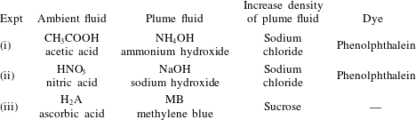
(figure 1). Before the beginning of each experiment, the tank was filled with a dilute aqueous solution of an acid: (i) acetic, (ii) nitric, or (iii) ascorbic acid were used to investigate the effects of different reactions (see table 1). To study the impacts of different source conditions, two round nozzles of radius 0.6 and 1.2 mm were used in the experiments. During each experiment, one of the nozzles was placed at the top of the tank and was connected to a glass beaker containing an aqueous solution of (i) ammonium hydroxide, (ii) sodium hydroxide, or (iii) methylene blue (see table 1). To increase the density of the source fluid in the beaker relative to that of the fluid in the tank, either sodium chloride or sucrose was added to the solution (see table 1). In experiments (i) and (ii), a few drops of phenolphthalein colour indicator were added to the clear fluid in the beaker (see table 1); the addition of the indicator did not affect the density or viscosity of the fluid. Owing to the presence of methylene blue in the solution, no extra dye was added to the fluid in the beaker in experiments (iii).
Reactive systems used in the experiments.
Conditions for experiments (i): ammonium hydroxide and acetic acid (see § 3.1). Here
 $Q_{0}$
(m
 $^{3}$
s
 $^{-1}$
) denotes the source volume flux;
 $r_{0}$
(m) is the radius of the nozzle;
 $\unicode[STIX]{x1D70C}_{b}^{0}/\unicode[STIX]{x1D70C}_{a}$
is the ratio between the density of the plume fluid at the source and that of the ambient fluid;
 $B$
(
 $\text{m}^{4}~\text{s}^{-3}$
) is the buoyancy flux;
 $\unicode[STIX]{x1D6E4}_{0}$
is the Morton number at the source (see appendix A);
 $L_{M_{0}}$
(m) is the length scale for the near-source region in which the flow is affected by the supplied momentum flux (see appendix A);
 $C_{a}$
(M) is the concentration of acetic acid in the ambient fluid;
 $C_{b}^{0}$
(M) is the concentration of ammonium hydroxide in the plume fluid at the source;
 $D_{s}$
is the stoichiometric dilution coefficient given by (5.12); and
 $L_{s}$
(m) is the stoichiometric length scale given by (5.13). In our calculations, we use
 $\unicode[STIX]{x1D708}=1.0\times 10^{-6}~\text{m}^{2}~\text{s}^{-1}$
as the kinematic viscosity of water at
 $20\,^{\circ }\text{C}$
(Atkins Reference Atkins1978). In all experiments, the Reynolds number at the source is
 $Re_{0}=1061$
, the Schmidt number associated with the plume fluid is
 $Sc_{b}=502$
(Perry & Green Reference Perry and Green2008), and that associated with the ambient fluid is
 $Sc_{a}=829$
(Vitagliano & Lyons Reference Vitagliano and Lyons1956).

Conditions for experiments (ii): sodium hydroxide and nitric acid (see § 3.2). In all experiments, the Reynolds number at the source is
 $Re_{0}=1061$
, the Schmidt number associated with the plume fluid is
 $Sc_{b}=517$
(Noulty & Leaist Reference Noulty and Leaist1984), and that associated with the ambient fluid is
 $Sc_{a}=337$
(Yeh & Wills Reference Yeh and Wills1971).

Conditions for experiments (iii): methylene blue and ascorbic acid (see § 3.3). In all experiments, the Reynolds number at the source is
 $Re_{0}=1061$
, the Schmidt number associated with the plume fluid is
 $Sc_{b}=1209$
(Leaist Reference Leaist1988), and that associated with the ambient fluid is
 $Sc_{a}=880$
(Shamim & Baki Reference Shamim and Baki1980).

During each experiment, the relatively dense fluid in the beaker was supplied to the tank using a peristaltic pump at a controlled flow rate
 $Q_{0}$
in the range
 $(1{-}2)\times 10^{-6}~\text{m}^{3}~\text{s}^{-1}$
(see tables 2–4). On entering the tank, the outflow from the nozzle rapidly became turbulent (see appendix A), and formed a dense plume that descended through the surrounding ambient fluid. The tank was backlit using a light panel of dimensions
 $50~\text{cm}\times 80~\text{cm}$
(manufactured by Electro-LuminX Lighting Co.) positioned at the rear of the tank (see figure 1). A Nikon D300 camera, located in front of the tank, was used to capture pictures at a frequency of 5 Hz (figure 2
a). Each image had 2136 pixels in the horizontal direction and 3212 pixels in the vertical direction, resulting in a resolution of
 $0.218~\text{mm}~\text{pixel}^{-1}$
. The experiments were performed in a dark room, and so the only light detected by the camera had been transmitted through the fluid in the tank. While passing through the tank during an experiment, the light was attenuated by the dyed plume fluid. For sufficiently low concentrations of dye, the light attenuation produced by a unit volume of dyed fluid was linearly proportional to the concentration of dye in the fluid (see figure 3; cf. Allgayer & Hunt Reference Allgayer and Hunt2012), and so the line-of-sight average concentration of dye in the plume could be inferred based on the distribution of the light attenuation in the images (figure 2
b). Each experiment typically lasted 2.5–3 min, during which approximately 750–900 photographs were captured. A time average of these photographs was calculated for each experiment to estimate the average distribution of the dye concentration in the plume during the experiment (figure 2
c). In order to ensure that the results are repeatable and reproducible, each reactive experiment was repeated up to three times. In figures 4, 7, 10 and 11 we show the different results obtained when repeating experiment 5; these results are labelled ‘5a’, ‘5b’ and ‘5c’. For all other experiments, we plot the average of the results obtained from each run. For calibration purposes, and in order to compare the properties of a plume with chemical reaction to those of an inert plume, each reactive experiment was also repeated using fresh water as the ambient fluid in the tank.
(a) Photograph of an inert plume descending through fresh water. (b) The depth-averaged concentration of dye in the plume is visualised using false colours. (c) Time- and depth-averaged concentration of dye in the plume. This image has been obtained by averaging 200 photographs which were captured during 40 s over the course of the experiment.

Light attenuation produced by an aqueous solution of (a) phenolphthalein and (b) methylene blue dye. A 2 cm thick cell containing the dyed fluid was positioned in front of the experimental light sheet (see § 2.1). Different dye concentrations were tested, ranging between 0 and 0.2 ppm. The fraction
 $\unicode[STIX]{x1D6F7}$
of light absorbed by the dyed fluid was measured using the experimental set-up described in § 2.1. Each experiment was repeated three times.

2.2 Turbulent plumes in fresh water
The outcomes of the inert experiments were analysed first, in order to: (i) estimate the errors associated with the light attenuation experimental technique; (ii) identify the virtual origin of the plume and estimate its entrainment coefficient; and (iii) measure the time-averaged light attenuation produced by the plume fluid as it becomes increasingly diluted while descending through the tank.
In a steady-state plume descending through an inert unstratified ambient, the buoyancy flux
 $$\begin{eqnarray}B=2\unicode[STIX]{x03C0}\int _{0}^{\infty }\frac{\unicode[STIX]{x1D70C}-\unicode[STIX]{x1D70C}_{a}}{\unicode[STIX]{x1D70C}_{a}}\,rgw\,\text{d}r\end{eqnarray}$$
is conserved (Morton et al.
Reference Morton, Taylor and Turner1956); here,
 $\unicode[STIX]{x1D70C}$
and
 $\unicode[STIX]{x1D70C}_{a}$
(kg m
 $^{-3}$
) are the densities of the plume and the ambient fluids, respectively,
 $r$
(m) is the radial distance of a parcel of fluid from the plume centreline,
 $g$
(m s
 $^{-2}$
) is the gravitational acceleration, and
 $w$
(m s
 $^{-1}$
) is the downward speed of the plume fluid. In order to estimate the errors associated with the image analysis technique, the photographs captured during each inert experiment were used to quantify the flux of dye in the plume as a function of distance from the source,
 $F(z)$
, and verify whether this flux was conserved. Figure 4 illustrates how
 $F(z)$
was measured. For each picture captured during an experiment, we measured the horizontally averaged profile of dye concentration in the plume. A time series of these profiles is plotted in figure 4(a): dark fronts stretching diagonally are observed in this image, illustrating the downward motion of the plume eddies over time. We used the Hough transform as available in MATLAB to identify the fronts (red lines in figure 4
a), measure their gradients, and thereby estimate the mean speed of the eddies as a function of distance below the source,
 $u_{e}(z)$
(cf. Mingotti & Woods Reference Mingotti and Woods2016). Figure 4(b) shows that our estimates were in good agreement with the expected speed of the plume fluid based on Morton et al. (Reference Morton, Taylor and Turner1956). Finally, we multiplied each cross-sectional dye concentration profile by the associated speed profile to infer the magnitude of the flux of dye in the plume,
 $F(z)$
. Figure 4(c) shows that, across a number of experiments, the time-averaged fluxes of dye in the plume were approximately conserved, with fluctuations of the order of 5 %–7 % about the mean value
 $\bar{F}$
. This confirms that in our experiments the attenuation of the light produced by a unit volume of dyed fluid in the tank was proportional to the concentration of dye in the fluid (see figure 3), and the errors associated with the image analysis technique were of the order of 5 %–7 %.
(a) Time series of the horizontally averaged profiles of dye concentration in the plume. (b) The measured profiles of the time-averaged eddy velocity,
 $u_{e}(z)$
, compared with the expected top-hat speed profiles,
 $u_{e_{ref}}(z)$
(Morton et al.
Reference Morton, Taylor and Turner1956). (c) Each measured flux of dye in the plume,
 $F(z)$
, is scaled by the vertically averaged mean flux,
 $\bar{F}$
. It is seen that
 $F(z)$
is approximately constant in the tank, with deviations of the order of 5 %–7 % associated with the limitations of the image analysis technique. In panels (b) and (c), the vertical distance below the source,
 $z$
, is scaled by the height of the tank,
 $H$
(m). Error bars are plotted for experiment 6 (see table 2).

Plume theory indicates that, in the absence of any chemical reaction, the reduced gravity of the plume fluid
 $g^{\prime }$
and the plume radius
 $b$
vary with distance from the source,
 $z$
(Morton et al.
Reference Morton, Taylor and Turner1956) according to
 $$\begin{eqnarray}g^{\prime }(z+z_{0})=\frac{B}{Q(z+z_{0})}\propto B^{2/3}(z+z_{0})^{-5/3}\end{eqnarray}$$
and
 $$\begin{eqnarray}b(z+z_{0})={\textstyle \frac{6}{5}}\unicode[STIX]{x1D6FC}(z+z_{0}),\end{eqnarray}$$
respectively. Here, top-hat radial profiles are assumed (cf. Morton et al.
Reference Morton, Taylor and Turner1956; Papanicolau & List Reference Papanicolau and List1988), while
 $z_{0}$
(m) denotes the vertical distance between the actual source and the virtual source of the plume (Hunt & Kaye Reference Hunt and Kaye2001) and
 $\unicode[STIX]{x1D6FC}$
is the entrainment coefficient (Morton et al.
Reference Morton, Taylor and Turner1956). Two filling-box inert experiments were carried out in the tank using the method described by Linden, Lane-Serff & Smeed (Reference Linden, Lane-Serff and Smeed1990) to measure
 $z_{0}=(5.2\pm 0.3)\times 10^{-3}$
m and
 $\unicode[STIX]{x1D6FC}=0.10\pm 0.02$
(see appendix A). Our estimates of both
 $z_{0}$
and
 $\unicode[STIX]{x1D6FC}$
are in good agreement with the literature (e.g. Bower et al.
Reference Bower, Caulfield, Fitzgerald and Woods2008).
3 Reactive systems
3.1 Fast reaction between acetic acid and ammonium hydroxide
Two sets of experiments have been carried out to explore the behaviour of plumes with a fast chemical reaction. In the first set, an aqueous solution of acetic acid was used as the ambient fluid in the tank, and a solution of ammonium hydroxide was used as the plume fluid (see tables 1 and 2). The concentrations of chemicals used in this set of experiments are listed in table 2 and discussed in appendix B. Within the range of concentrations used, the chemical reaction between acetic acid and ammonium hydroxide had negligible effects on the density of the solutions (Domingos & Cardoso Reference Domingos and Cardoso2015), and did not affect the entrainment coefficient
 $\unicode[STIX]{x1D6FC}$
(see § 2.2 and appendix A). Inert sodium chloride was added to the plume fluid to increase its density relative to the ambient fluid. The products of the reaction between acetic acid and ammonium hydroxide are ammonium acetate and water:

The rate law of this second-order reaction is

with
 $k_{r_{1}}\approx 10^{11}~\text{M}^{-1}~\text{s}^{-1}$
at
 $20\,^{\circ }\text{C}$
(Someya et al.
Reference Someya, Yoshida, Tabata and Okamoto2009). Acetic acid and ammonium hydroxide are a weak acid and a weak base, respectively, and therefore they are partly dissociated in their solutions, according to the following chemical equilibria (Housecroft & Constable Reference Housecroft and Constable2002)

and

It follows that the equilibrium constant for the reaction between acetic acid and ammonium hydroxide is given by

in which
 $K_{w}$
(M
 $^{2}$
) is the dissociation constant for ionised water,

Since the constant given by (3.5) is large, the reaction is product-favoured and driven practically to completion (Housecroft & Constable Reference Housecroft and Constable2002).
To observe the motion of the plume fluid in the tank and track the progress of the reaction, a few drops of phenolphthalein indicator were added to the solution of ammonium hydroxide and sodium chloride just before the beginning of each experiment. Phenolphthalein is a weak acid, which reacts according to the following equilibrium (Housecroft & Constable Reference Housecroft and Constable2002)

In (3.7), HInd is the colourless acidic form of phenolphthalein, while Ind
 $^{-}$
is the conjugate basic form, which is characterised by a pink/purple colour (Domingos & Cardoso Reference Domingos and Cardoso2015). Hence, an alkaline solution containing phenolphthalein is coloured; however, the colour fades when the pH of the solution decreases beyond neutralisation (Wittke Reference Wittke1983). The relationship between colour intensity and depletion of chemical is linear (Domingos & Cardoso Reference Domingos and Cardoso2015).
3.2 Fast reaction between nitric acid and sodium hydroxide
In the second set of experiments involving a fast reaction between the plume and the ambient fluid, a solution of nitric acid was used as the ambient fluid in the tank, and a solution of sodium hydroxide was used as the plume fluid (see tables 1 and 3). Within the range of concentrations used, the chemical reaction between nitric acid and sodium hydroxide did not affect the density of the solutions (Ulpre et al.
Reference Ulpre, Eames and Greig2013), nor the entrainment coefficient
 $\unicode[STIX]{x1D6FC}$
(see § 2.2 and appendix A). Just as in the first set of experiments, inert sodium chloride and a few drops of phenolphthalein indicator were added to the solution to control its density and colour. The products of the reaction are sodium nitrate and water (Ulpre et al.
Reference Ulpre, Eames and Greig2013):

Nitric acid and sodium hydroxide are a strong acid and a strong base, respectively, and therefore we expect them to be completely dissociated in their solutions. The reaction given in (3.8) is instantaneous (Atkins Reference Atkins1978).
(a,b) Instantaneous and (c,d) time-averaged concentrations of phenolphthalein dye in a plume of ammonium hydroxide descending through (a,c) fresh water or (b,d) a solution of acetic acid. A comparison of the time- and depth-averaged profiles of dye concentration along the plume’s centreline is given in (e).

3.3 Slower reaction between ascorbic acid and methylene blue
A third set of experiments was carried out to observe the behaviour of plumes with a slower chemical reaction. In these experiments, a solution of methylene blue was used as the plume fluid, while a solution of ascorbic acid was used as the ambient fluid in the tank (see tables 1 and 4). Within the range of concentrations used, the chemical reaction between ascorbic acid and methylene blue did not affect the density of the solutions (Domingos & Cardoso Reference Domingos and Cardoso2015), nor the entrainment coefficient
 $\unicode[STIX]{x1D6FC}$
(see § 2.2 and appendix A). Inert sucrose was added to the plume fluid to increase its density relative to the ambient fluid. The products of the reaction between methylene blue (MB) and ascorbic acid (H
 $_{2}$
A) are leucomethylene blue (LB) and dehydroascorbic acid (DHA):

Mowry & Ogren (Reference Mowry and Ogren1999) measured the rate law of this second-order reaction,

and found
 $k_{r_{2}}\approx 1\pm 0.2~\text{M}^{-1}~\text{s}^{-1}$
at
 $20\,^{\circ }\text{C}$
. Snehalatha, Rajanna & Saiprakash (Reference Snehalatha, Rajanna and Saiprakash1997) proposed two different mechanisms for the reaction between ascorbic acid and methylene blue. Both mechanisms are irreversible and second order. As a result of the irreversible reaction, the colour of a mixture of methylene blue and ascorbic acid gradually fades. In our experiments, we track the progress of the reaction in the plume by observing the change in the colour of the plume fluid (see § 5.2).
It should be noted that, for the reaction to produce significant effects within a relatively short time during each experiment, sufficiently large concentrations of ascorbic acid and methylene blue were used in this set of experiments (see table 4). At these concentrations, the colour of the plume fluid near the source was very dark, making it difficult to measure the concentration of dye in the plume eddies using the light attenuation technique in this region. However, the colour of the plume fluid rapidly became lighter as the fluid became increasingly dilute while descending through the tank. For this reason, in plotting figures 7(d), 9 and 12 (§§ 4 and 5), we will only consider the portion of the tank in which the concentration of dye in the plume fluid could be measured using the experimental technique described in § 2.
4 Experimental observations
Instantaneous images of a fast reaction, an alkaline plume descending through (a) fresh water and (b) an acidic environment: a rainbow colour map is used to illustrate the concentration of phenolphthalein dye in the plume. In (c) and (d), the same images are processed to highlight the descending eddies. A white/red colour map is used to highlight the regions of the plume in which the instantaneous dye concentration exceeds the time-averaged mean concentration.

4.1 Time-averaged concentration of the plume fluid
Figure 5 shows a side-by-side comparison of the outcomes of two experiments in which the same alkaline plume fluid descended through either fresh water or an acidic solution (experiment 1 in table 2). In figure 5(a,c), the tank was filled with fresh water. Both the instantaneous and the time-averaged images show that, while descending through the tank, the plume fluid became increasingly dilute as a result of the entrainment of ambient fluid. Figure 5(b,d) illustrate the results of an experiment in which the tank was filled with a solution of acetic acid. In this case, the plume was subjected to both dilution and chemical reaction, leading to a faster reduction in the pH of the fluid, which in turn resulted in a faster reduction in the concentration of dye in the fluid (figure 5 e).
The red line in figure 5(e) shows that at distances below the source greater than
 $z/H>0.7{-}0.8$
approximately, the plume in the reactive system produced a negligible amount of light attenuation through the tank. At this distance from the source, all the phenolphthalein dye contained in the supplied fluid had turned colourless, and this indicates that the pH of the fluid had decreased beyond neutralisation as a result of the chemical reaction (see § 2.1; cf. Wittke Reference Wittke1983).
Time-averaged mean (a,c) size of the parcels of reactive fluid relative to the size of the eddies in an inert plume,
 $D_{r}/D_{i}$
, and (b,d) concentration of dye per unit volume in a parcel of reactive fluid relative to the concentration in a parcel of inert plume fluid,
 $C_{r}/C_{i}$
, for (a,b) fast and (c,d) slow reactions. All data are presented as a function of the distance from the plume source,
 $z$
, scaled by the tank’s height,
 $H$
. In (a) and (b), error bars are plotted for experiment 6 (see table 2), while in (c) and (d) error bars are plotted for experiment 19 (see table 4). In (a,b) the variation between the results of different experiments is larger at small distances below the source,
 $z/H<0.05{-}0.01$
(i.e.
 $z<3.5$
–7 cm below the nozzle approximately, see tables 2 and 3). In this near-source region, the flow in the plume is still transitional or just settling into full turbulence. It should be noted that the magnitude of the discrepancies between the results depicted in (a) and (b) is typically smaller than the expected errors associated with the image analysis technique, as discussed in § 2.

4.2 Distribution and concentration of the reactive fluid in plume eddies
While comparing the time-averaged concentration profiles depicted in figure 5(e) enables us to identify the distance from the source at which the chemical reaction is complete, we should note that turbulent plumes are effectively composed of transient or intermittent eddies (Mingotti & Woods Reference Mingotti and Woods2015a ,Reference Mingotti and Woods b ). It is interesting to observe how the concentration of the reactants varies in the eddies as a function of distance from the source and of the reaction rate.
In figure 6(a), we use false colours to illustrate the concentration of phenolphthalein dye in a plume that descends through fresh water. In order to identify the turbulent eddies in this picture, we first subtract the time-averaged mean concentration of dye from the instantaneous concentration depicted in the image. We then use a red colour map to illustrate the fractional amplitude of the fluctuations above the mean (figure 6
c). We measure the horizontal equatorial length or diameter of each eddy in the plume as a function of distance from the source. We observe that, as the inert plume fluid descends through fresh water, the time-averaged mean diameter of the eddies,
 $D_{i}$
, increases with distance from the source due to the entrainment of ambient fluid (figure 6
c), while the mean concentration of dye in the eddies,
 $C_{i}$
, decreases as a result of dilution (figure 6
a).
We repeat the same analysis for all the images captured during each experiment: as an example, figure 6(b,d) show the results obtained when processing one of the pictures captured during experiment 1 (fast reaction, see table 2). Using these figures, we measure the equatorial diameter,
 $D_{r}$
, and concentration,
 $C_{r}$
, of each parcel of dyed fluid in the reactive plume. Figure 7 illustrates the results of our measurements. It is seen that the mean diameter of the parcels of dyed fluid in a plume with a fast chemical reaction is similar to that of the eddies of an inert plume near the source; however, the ratio
 $D_{r}/D_{i}$
decreases progressively with distance from the source (figure 7
a). On the other hand, we observe that the mean concentration of phenolphthalein indicator in a unit volume of dyed fluid in a plume with a fast chemical reaction is approximately equal to that produced by a unit volume of dyed fluid in an inert plume at all distances from the source,
 $C_{r}/C_{i}\approx 1$
(figure 7
b).
The results obtained when analysing the pictures captured during the slow reaction experiments are different. Figure 7(c) shows that the size of the parcels of dyed fluid in a plume with a slow reaction was similar to that of the eddies in an inert plume at all distances from the source in our experiments,
 $D_{r}/D_{i}\approx 1$
. On the other hand, the concentration of methylene blue dye in a plume with a slow reaction decreased progressively with distance from the source relative to that in an inert plume,
 $C_{r}/C_{i}<1$
(figure 7
d).
Cartoon illustrating the different distributions of reactants in the two cases of a fast and slow chemical reaction.

These experimental observations suggest that the process of consumption of the chemical species in a plume with a fast reaction is different from that in a plume with a slower reaction (see figure 8). When the time required for the reaction to develop is smaller than the time required for a parcel of dyed plume fluid to mix with the entrained fluid, then the reaction primarily takes place near the edges of the parcel (dashed black lines in figure 8
b). In this border region, the dyed fluid mixes locally with the entrained fluid: as the two fluids react, the colour of the dyed fluid rapidly fades. This leads to a reduction in the diameter of the parcel of dyed reactive fluid,
 $D_{r}$
, as illustrated in figure 7(a). The fluid in the core of the parcel, however, is not affected by the fast chemical reaction, and so its concentration
 $C_{r}$
is only subjected to the effects of dilution: hence,
 $C_{r}$
decreases with distance from the source at a rate similar to that of the concentration of dye in an inert plume,
 $C_{i}$
(see figure 7
b).
On the other hand, in the case of a slower reaction, the time required for the convective mixing of the entrained fluid into an eddy is shorter than the time required for the reaction to develop. In this situation, the entrained reactants are continuously distributed throughout the entire volume of the eddy,
 $D_{r}\sim D_{i}$
(figures 7
c and 8
c). The fluid in the bulk of the eddy is consequently subjected to the effects of both dilution and reaction, and so
 $C_{r}$
decreases more rapidly than
 $C_{i}$
with distance from the source (see figure 7
d).
Motivated by these experimental results, in the next section we develop a simple model based on plume theory to quantify the concentration of the supplied reactants in the plume fluid as a function of distance from the source. We then test the model by comparing the outcome of the experiments with the model predictions.
5 Model
In this section, plume theory is used to build a model that quantifies the concentration of reactants in the plume fluid as a function of distance from the source in the two limiting cases of a slow and of an instantaneous reaction. In § 5.1, we compare the length and time scales that govern the processes of entrainment, dilution and chemical reaction within the plume, and identify the parameters that control the progress of slow and fast chemical reactions in the plume. In § 5.2, we focus on slow reactions, and quantify the concentration of the supplied reactants in the plume fluid as a function of time and distance from the source. In § 5.3, we focus on fast reactions. We estimate the fraction of the entrained fluid that mixes and reacts within the plume as a function of distance from the source. In the limit of an instantaneous reaction, we calculate the distance at which the reaction is complete.
5.1 Slow and fast chemical reactions in a turbulent plume
5.1.1 Entrainment of ambient fluid
Plume theory indicates that, as a result of entrainment of ambient fluid, the plume volume flux,
 $Q$
(m
 $^{3}$
s
 $^{-1}$
), increases with distance from the source,
 $z$
(Morton et al.
Reference Morton, Taylor and Turner1956) as
 $$\begin{eqnarray}Q=\unicode[STIX]{x1D706}B^{1/3}z^{5/3},\end{eqnarray}$$
where
 $B$
(
 $\text{m}^{4}~\text{s}^{-3}$
) is the buoyancy flux and
 $$\begin{eqnarray}\unicode[STIX]{x1D706}={\textstyle \frac{6}{5}}\unicode[STIX]{x1D6FC}({\textstyle \frac{9}{10}}\unicode[STIX]{x1D6FC})^{1/3}\unicode[STIX]{x03C0}^{2/3}\end{eqnarray}$$
is a universal constant dependent on the entrainment coefficient
 $\unicode[STIX]{x1D6FC}$
(Linden et al.
Reference Linden, Lane-Serff and Smeed1990). Both the plume radius
 $b$
and the mean diameter of the eddies in the plume increase linearly with distance from the source (Papanicolau & List Reference Papanicolau and List1988). Consequently, the mean top-hat speed of the fluid,
 $u$
(m s
 $^{-1}$
), decreases with distance from the source as
 $$\begin{eqnarray}u=\frac{Q}{\unicode[STIX]{x03C0}b^{2}}\sim \unicode[STIX]{x1D6FC}^{-2}\unicode[STIX]{x1D706}B^{1/3}z^{-1/3}.\end{eqnarray}$$
It follows that the turbulent motion of the plume fluid and the entrainment of ambient fluid into the plume are governed by the following length and time scales (cf. table 5):
 $$\begin{eqnarray}L_{e}=\unicode[STIX]{x1D6FC}z\end{eqnarray}$$
and
 $$\begin{eqnarray}\unicode[STIX]{x1D70F}_{e}=\frac{L_{e}}{u}=\unicode[STIX]{x1D6FC}^{3}\unicode[STIX]{x1D706}^{-1}B^{-1/3}z^{4/3}.\end{eqnarray}$$
Length and time scales used in the model.

5.1.2 Time scale for stoichiometric dilution of the supplied fluid
We let
 $Q_{0}$
(m
 $^{3}$
s
 $^{-1}$
) denote the plume volume flux at the source. We assume that the supplied fluid contains an alkaline solution, MOH, and we let
 $C_{b}^{0}$
(M) denote the initial concentration of this solution. As the plume descends through the surrounding ambient, the supplied fluid is diluted through the addition of a volume flux
 $Q_{e}$
of entrained acid, HA, of a uniform concentration
 $C_{a}$
. As indicated by Ulpre et al. (Reference Ulpre, Eames and Greig2013), the chemical reaction between the fluids is governed by the conservation of charge

and by the conservation of mass of acid and alkali, respectively,

and

We let
 $K_{a}$
and
 $K_{b}$
(M) denote the dissociation constants of the acidic and of the alkaline solutions, respectively,

and

We define the dilution coefficient
 $D$
as the ratio between the volume flux of the entrained fluid and that of the supplied fluid at a given distance from the source. Using a combination of (5.7)–(5.10), this coefficient is given by

As the volume flux of entrained fluid increases with distance from the source, the number of moles of entrained acid and the dilution coefficient also increase. We let
 $D_{s}$
denote the critical stoichiometric dilution at which the supplied alkali and entrained acid are present in the plume in stoichiometric amounts. At this critical dilution, the mean concentration of hydrogen ions equals that of hydroxide ions in the solution,
 $[\text{H}^{+}]=[\text{OH}^{-}]$
, and so using (3.6) and (5.6) we obtain
 $$\begin{eqnarray}D_{s}=\frac{C_{b}^{0}K_{b}(K_{a}+K_{w}^{1/2})}{C_{a}K_{a}(K_{b}+K_{w}^{1/2})}.\end{eqnarray}$$
Using a combination of (5.1) and (5.12), we calculate that the distance between the plume source and the level at which the stoichiometric dilution is achieved is given by
 $$\begin{eqnarray}L_{s}=\unicode[STIX]{x1D706}^{-3/5}Q_{0}^{3/5}B^{-1/5}(1+D_{s})^{3/5}\end{eqnarray}$$
as listed in table 5. Equations (5.3) and (5.13) are then used to estimate that the time required for the plume fluid to flow from the source to the stoichiometric level scales by
 $$\begin{eqnarray}\unicode[STIX]{x1D70F}_{s}=\frac{L_{s}}{u}=\unicode[STIX]{x1D6FC}^{2}\unicode[STIX]{x1D706}^{-8/5}Q_{0}^{3/5}B^{-8/15}z^{1/3}(1+D_{s})^{3/5}.\end{eqnarray}$$
5.1.3 Time scale for chemical reaction
In our experiments, the volumetric flow rate of ambient fluid entrained into the plume becomes larger than that of source fluid at short distances from the source. The concentration of the ambient chemical species in the plume is therefore approximately constant in the plume, and the chemical reaction between the source and the entrained fluid may be treated as a pseudo-first-order reaction (Domingos & Cardoso Reference Domingos and Cardoso2015). The time scale for a change in the concentration of the chemical species in the plume fluid is therefore given by (see table 5)
 $$\begin{eqnarray}\unicode[STIX]{x1D70F}_{r}=(k_{r}C_{a})^{-1},\end{eqnarray}$$
while the distance travelled by the plume fluid during this time scales as
 $$\begin{eqnarray}L_{r}=u\unicode[STIX]{x1D70F}_{r}=\unicode[STIX]{x1D6FC}^{-2}\unicode[STIX]{x1D706}B^{1/3}z^{-1/3}(k_{r}C_{a})^{-1}.\end{eqnarray}$$
We compare the time scale for achieving the stoichiometric dilution,
 $\unicode[STIX]{x1D70F}_{s}$
, with the reaction time scale,
 $\unicode[STIX]{x1D70F}_{r}$
, in our experiments. In the slow reaction experiments (see § 3.3 and table 4), the ratio
 $\unicode[STIX]{x1D70F}_{s}/\unicode[STIX]{x1D70F}_{r}$
is typically of the order of
 $10^{-3}{-}10^{-2}$
. This indicates that the plume rapidly entrains a large amount of ambient fluid while descending to the stoichiometric level
 $L_{s}$
; however, the chemical reaction is comparatively slow. Hence, we expect the consumption of the supplied chemicals to be controlled by the reaction time scale (see table 5), and most of the effects of the reaction to be visible at distances larger than
 $L_{s}$
. On the other hand, in our fast reaction experiments (see §§ 3.1 and 3.2 and tables 2 and 3),
 $\unicode[STIX]{x1D70F}_{s}/\unicode[STIX]{x1D70F}_{r}$
is typically of the order of
 $10^{7}{-}10^{8}$
. This suggests that as soon as a parcel of acidic fluid is entrained from the ambient and mixed within the plume, it immediately reacts with the descending fluid. Hence, we expect the consumption of the supplied chemicals to be controlled by the entrainment and mixing time scales (see table 5), and most of the effects of the reaction to be visible at distances smaller than
 $L_{s}$
.
5.2 Consumption of the chemical species in a plume with a slow reaction
In this section, we focus on slow reactions and quantify the concentration of the supplied chemicals in the plume fluid as a function of distance from the source. Both dilution and reaction lead to a gradual reduction in the concentration of the supplied chemical species
 $C_{b}$
(cf. Domingos & Cardoso Reference Domingos and Cardoso2013). Using (5.1) and (5.15), this concentration varies with time according to
 $$\begin{eqnarray}\frac{\text{d}C_{b}}{\text{d}t}=-\frac{5}{4}\frac{C_{b}}{t}-\frac{C_{b}}{\unicode[STIX]{x1D70F}_{r}}.\end{eqnarray}$$
The ratio between the concentration in a reactive system (
 $C_{a}>0,~\unicode[STIX]{x1D70F}_{r}>0$
) and that in an inert system (
 $C_{a}=0,~\unicode[STIX]{x1D70F}_{r}\rightarrow \infty$
) is then
 $$\begin{eqnarray}\frac{C_{b,reaction}}{C_{b,inert}}=\exp \!\left(-\frac{t}{\unicode[STIX]{x1D70F}_{r}}\right).\end{eqnarray}$$
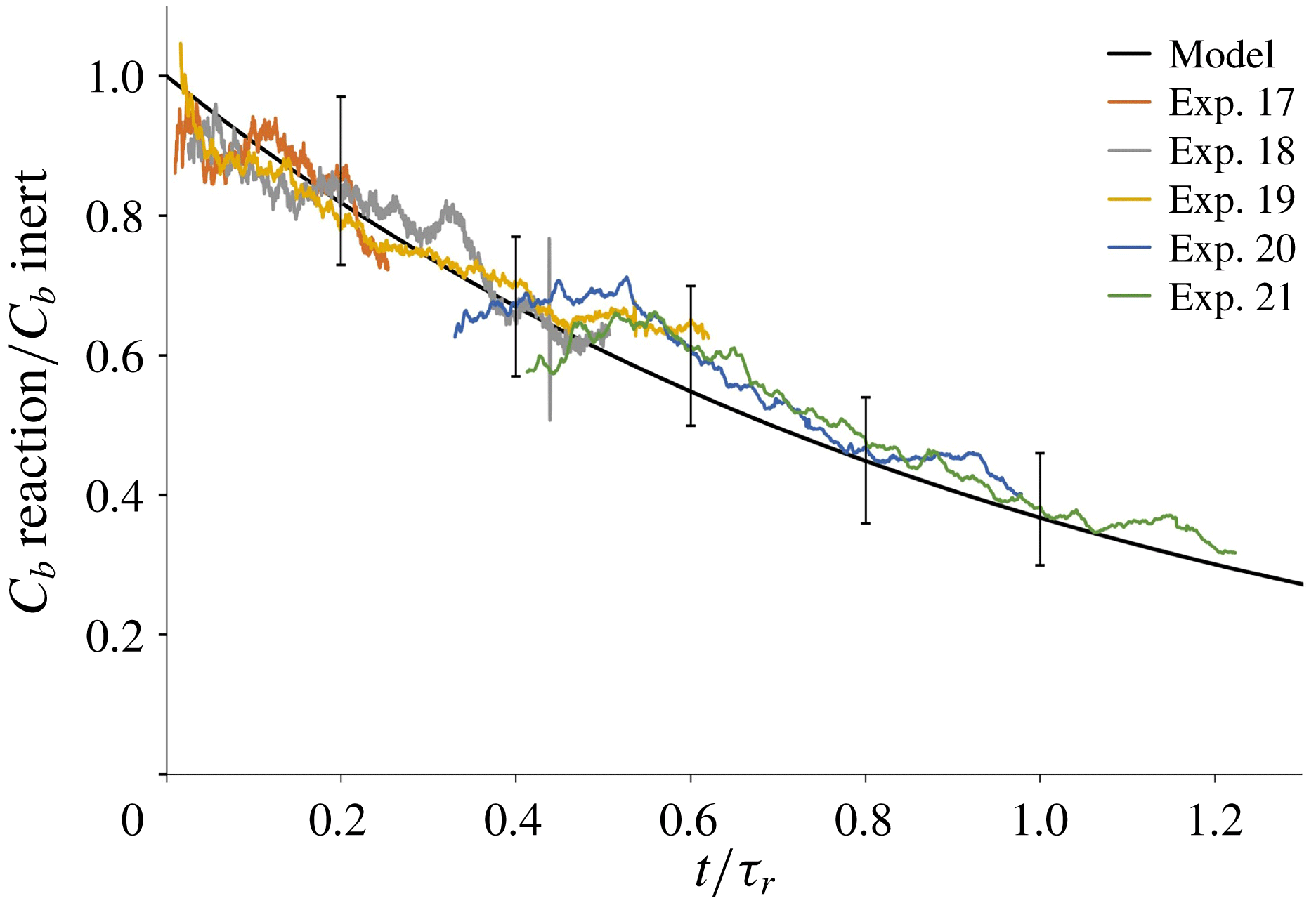
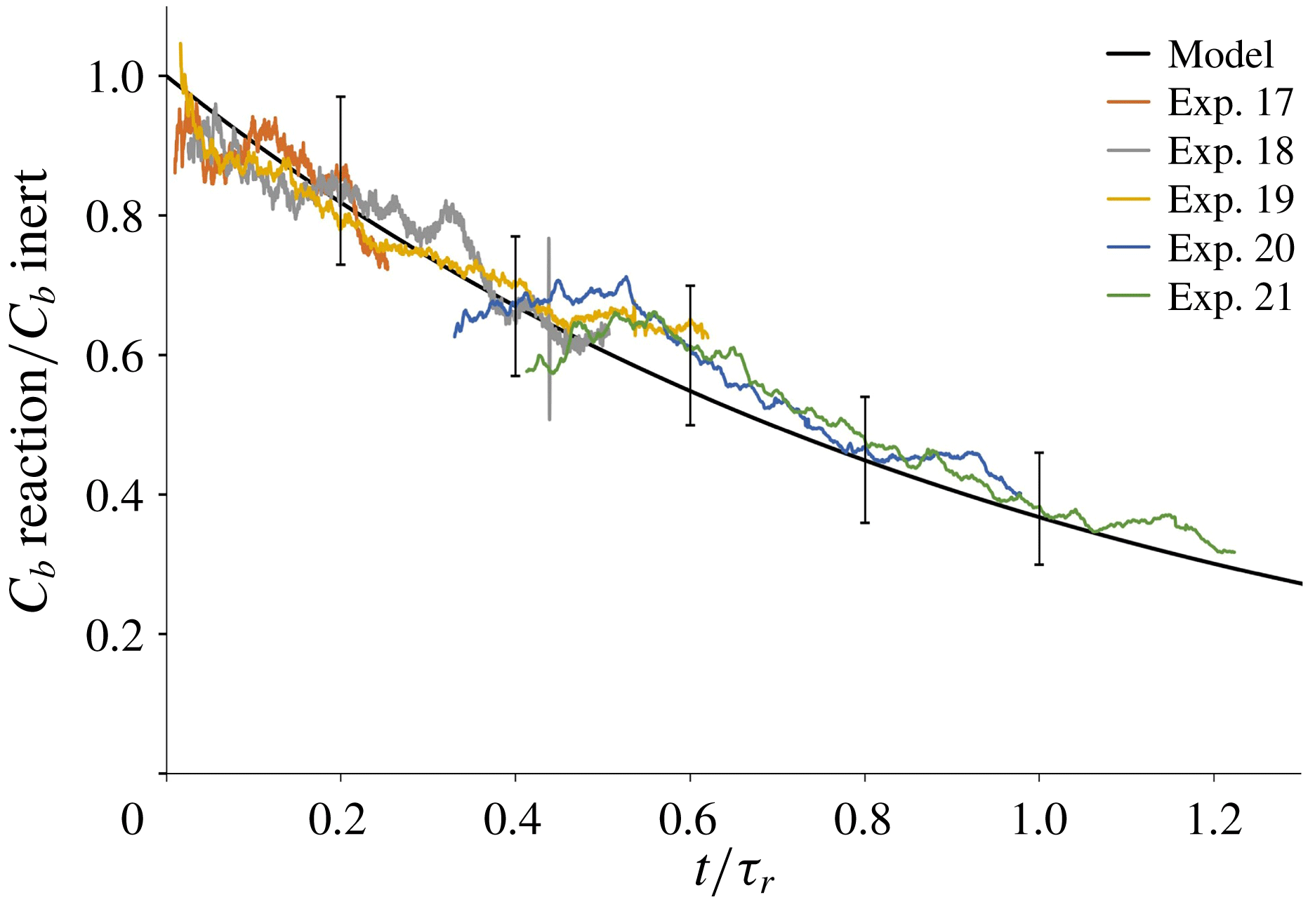
Our model of the consumption of reactants in a plume with a slow chemical reaction is tested against the results of the laboratory experiments described in § 3.3. For each of the experiments listed in table 4, we calculate the ratio between the time-averaged light attenuation produced by a methylene blue plume that descends through an acidic environment, and that produced by the associated inert plume that descends through fresh water (cf. figure 7 d). Figure 9 shows that the model prediction (black line, based on (5.18)) is in good agreement with the results of the experiments, with deviations of the order of 10 %, which are compatible with the expected errors associated with the image processing technique (see § 2.2).
5.3 Consumption of the chemical species in a plume with a fast reaction
We now consider the case of a fast reaction between the supplied and the entrained fluid in the plume. In the limit
 $\unicode[STIX]{x1D70F}_{s}/\unicode[STIX]{x1D70F}_{r}\gg 1$
, we assume the reaction to be instantaneous (
 $\unicode[STIX]{x1D70F}_{r}=L_{r}=0$
), and the supplied chemical species to be progressively consumed in the region
 $0<z<L_{s}$
as an increasing flux of ambient fluid is entrained and mixed within the plume.
5.3.1 Time scale for mixing at the Batchelor scale
Domingos & Cardoso (Reference Domingos and Cardoso2015) previously observed non-uniform distributions of reactants in single-phase thermals with a fast reaction, and found the progress of the reaction to be controlled by the local mixing of the reactive fluids. Similarly, in § 4.2 we observed that sufficiently fast reactions may develop only in a portion of the plume’s volume, with chemically active regions near the edges of each parcel of reactive fluid, and inactive regions in the core of each parcel of fluid (see figure 8
b). Based on these experimental observations and on the previous findings by Domingos & Cardoso, we let
 $\unicode[STIX]{x1D70F}_{m}$
denote the time scale for the local mixing of the fluids at the Batchelor scale. For sufficiently large Reynolds and Schmidt numbers associated with the plume flow (see tables 2 and 3; cf. Fox Reference Fox2003), this time scale is given by
 $$\begin{eqnarray}\unicode[STIX]{x1D70F}_{m}={\textstyle \frac{1}{2}}\ln Sc_{b}\cdot \unicode[STIX]{x1D70F}_{e}Re^{-1/2}\sim \ln Sc_{b}\cdot \unicode[STIX]{x1D6FC}^{7/2}\unicode[STIX]{x1D706}^{-3/2}\unicode[STIX]{x1D708}^{1/2}B^{-1/2}z,\end{eqnarray}$$
in which
 $Sc_{b}$
is the Schmidt number associated with the plume (see tables 2 and 3),
 $\unicode[STIX]{x1D708}$
(
 $\text{m}^{2}~\text{s}^{-1}$
) is the kinematic viscosity of the mixture (Pope Reference Pope2000; Kundu, Cohen & Dowling Reference Kundu, Cohen and Dowling2015) and
 $$\begin{eqnarray}Re=\frac{uL_{e}}{\unicode[STIX]{x1D708}}=\unicode[STIX]{x1D6FC}^{-1}\unicode[STIX]{x1D706}\unicode[STIX]{x1D708}^{-1}B^{1/3}z^{2/3}\end{eqnarray}$$
is the Reynolds number associated with the plume eddies. For each of our experiments, we calculate
 $\unicode[STIX]{x1D70F}_{m}$
as a function of distance from the source using (5.19) and the experimental measurements of the speed and size of the eddies in the plume (see § 2.2). Figure 10(a) shows that the time required for the turbulent convection of the fluid in an eddy is always much larger than the time required for the local mixing of the fluid at the Batchelor scale in our experiments,
 $\unicode[STIX]{x1D70F}_{e}\gg \unicode[STIX]{x1D70F}_{m}$
. Hence, we expect that fast chemical reactions will develop primarily at this latter scale, and that the depth of the chemically active region in the periphery of each parcel of reactive fluid will be controlled by the Batchelor length scale,
 $L_{m}$
(Batchelor Reference Batchelor1959; Fox Reference Fox2003):
 $$\begin{eqnarray}L_{m}=Sc_{b}^{-1/2}L_{e}Re^{-3/4}=Sc_{b}^{-1/2}\unicode[STIX]{x1D6FC}^{7/4}\unicode[STIX]{x1D706}^{-3/4}\unicode[STIX]{x1D708}^{3/4}B^{-1/4}z^{1/2}.\end{eqnarray}$$
For each experiment with a fast reaction,
 $L_{m}$
is estimated using (5.21) and the experimental measurements of the time-averaged speed and size of the eddies in the plume (see § 2.2). In figure 10(b,c), we compare
 $L_{m}$
with the mean diameters of the eddies,
 $D_{i}$
, and of the parcels of reactive fluid in our experiments,
 $D_{r}$
(see figure 6). It is seen that, in the region
 $0<z<L_{s}$
, the Batchelor length scale is much smaller than both diameters: this is consistent with our experimental observation of the chemical reaction developing in a relatively thin region near the edge of each parcel of reactive fluid in the plume (see figure 8
b). The mixture of ambient and entrained fluid in this region rapidly becomes neutralised, leading to a reduction in the parcel’s size (see figure 7). As a result of the slower process of large-scale mixing, some of the neutralised fluid is subsequently entrained and diluted into the core of the parcel of fluid; however, we expect that no chemical reaction will develop there.
Experimental measurements of (a) the ratio between the time scale for convective mixing of the fluid in an eddy and the Batchelor time scale,
 $\unicode[STIX]{x1D70F}_{e}/\unicode[STIX]{x1D70F}_{m}$
(Batchelor Reference Batchelor1959; Fox Reference Fox2003); (b) the ratio between the time-averaged mean diameter of the eddies and the Batchelor length scale,
 $D_{i}/L_{m}$
; and (c) the ratio between the time-averaged mean diameter of the parcels of reactive fluid and the Batchelor length scale,
 $D_{r}/L_{m}$
. All data are presented as a function of the distance from the virtual origin of the plume, scaled by
 $L_{s}$
(5.13).

5.3.2 Critical distance
 $z_{crit}$

Using (5.19) and (5.21), we estimate that the volume flux of fluid that is mixed within the plume by a micro-scale eddy in a unit of time, herein denoted by
 $Q_{m}$
, scales by
 $$\begin{eqnarray}\frac{\text{d}Q_{m}}{\text{d}t}\sim \frac{L_{m}^{3}}{\unicode[STIX]{x1D70F}_{m}^{2}}=\frac{\unicode[STIX]{x1D6FC}^{-7/4}\unicode[STIX]{x1D706}^{3/4}\unicode[STIX]{x1D708}^{5/4}B^{1/4}z^{-1/2}}{Sc_{b}^{3/2}(\ln Sc_{b})^{2}}.\end{eqnarray}$$
In turn, plume theory indicates that the volume flux of ambient fluid that is entrained into the plume by a macro-scale eddy in a unit of time scales by
 $$\begin{eqnarray}\frac{\text{d}Q}{\text{d}t}\sim \frac{L_{e}^{3}}{\unicode[STIX]{x1D70F}_{e}^{2}}=\unicode[STIX]{x1D6FC}^{-3}\unicode[STIX]{x1D706}^{2}B^{2/3}z^{1/3}.\end{eqnarray}$$
At all times, the volume flux of fluid that is mixed within the plume must be smaller than or equal to the volume flux of fluid that is entrained from the ambient. Using (5.22) and (5.23), we estimate that the fraction of the entrained volume flux that mixes and reacts with some of the supplied fluid in the plume decreases with distance from the source as
 $$\begin{eqnarray}\frac{\text{mixed volume flux}}{\text{entrained volume flux}}=\min \left(\frac{\unicode[STIX]{x1D6FC}^{5/4}\unicode[STIX]{x1D6FD}\unicode[STIX]{x1D706}^{-5/4}\unicode[STIX]{x1D708}^{5/4}B^{-5/12}z^{-5/6}}{Sc_{b}^{3/2}(\ln Sc_{b})^{2}};~1\right),\end{eqnarray}$$
where
 $\unicode[STIX]{x1D6FD}$
is a dimensionless constant, which represents the effective number of micro-scale eddies involved in complete reaction of the chemicals per unit macro-scale eddy associated with the entrainment and large-scale mixing in the plume. Equation (5.24) indicates that a critical distance from the source exists, at which the volume flux of fluid that is entrained by the plume is equal to that mixed by the small-scale turbulence:
 $$\begin{eqnarray}z_{crit}=\left(\frac{\unicode[STIX]{x1D6FD}^{3}}{Sc_{b}^{2}(\ln Sc_{b})^{6}}\right)^{2/5}\frac{L_{m}^{2}}{L_{e}}.\end{eqnarray}$$
For
 $z<z_{crit}$
, the volume of fluid entrained by the plume is smaller than the maximum volume that can be mixed at the Batchelor scale: we therefore expect that all the fluid entrained by the plume will mix with a portion of the supplied plume fluid and react, but the overall progress of the reaction will be limited by the lack of entrained fluid. On the other hand, for
 $z>z_{crit}$
the volume of fluid that is entrained by the plume is larger than the maximum volume that can be mixed at the Batchelor scale: in this case, the reaction will only develop in a fraction of the entrained fluid due to incomplete mixing.
5.3.3 Progress of the reaction
Equation (5.25) suggests that in the case
 $z_{crit}<L_{s}$
, only a fraction of the entrained fluid will react with the supplied fluid in the region
 $z_{crit}<z<L_{s}$
. Consequently, the consumption of the chemical species will be reduced in this region, and the distance from the source at which the chemical reaction reaches completion,
 $z_{r}$
, will be larger than
 $L_{s}$
(5.13). To estimate this distance, we let
 $R$
denote the fraction of the supplied chemicals that are still reactive at a given distance from the source. Using (5.12), (5.24) and (5.25), we calculate that this fraction is given by
 $$\begin{eqnarray}R(z)=\left\{\begin{array}{@{}ll@{}}1-{\displaystyle \frac{Q(z)}{(1+D_{s})Q_{0}}}, & 0<z<z_{crit},\\ 1-{\displaystyle \frac{1}{(1+D_{s})Q_{0}}}\!\left(\!\unicode[STIX]{x1D706}B^{1/3}z_{crit}^{5/3}+\displaystyle \int _{z_{crit}}^{z}\!\frac{\unicode[STIX]{x1D6FC}^{5/4}\unicode[STIX]{x1D6FD}\unicode[STIX]{x1D708}^{5/4}B^{-5/12}\unicode[STIX]{x1D701}^{-5/6}}{\unicode[STIX]{x1D706}^{5/4}Sc_{b}^{3/2}(\ln Sc_{b})^{2}}\frac{\text{d}Q}{\text{d}\unicode[STIX]{x1D701}}\,\text{d}\unicode[STIX]{x1D701}\!\right), & z_{crit}<z<z_{r}.\end{array}\right.\end{eqnarray}$$
A combination of (5.1), (5.13) and (5.26) enables us to write
 $R$
as a function of the stoichiometric length scale,
 $L_{s}$
, and the critical distance,
 $z_{crit}$
:
 $$\begin{eqnarray}R(z)=\left\{\begin{array}{@{}ll@{}}1-\left({\displaystyle \frac{z}{L_{s}}}\right)^{5/3}, & 0<z<z_{crit},\\[3.0pt] 1+\left({\displaystyle \frac{z_{crit}}{L_{s}}}\right)^{5/3}-2\left({\displaystyle \frac{z}{L_{s}}}\right)^{5/6}\left({\displaystyle \frac{z_{crit}}{L_{s}}}\right)^{5/6}, & z_{crit}<z<z_{r}.\end{array}\right.\end{eqnarray}$$
Equation (5.27) indicates that the fraction of reactive chemicals in the plume decreases more rapidly in the region
 $0<z<z_{crit}$
, where all of the entrained fluid mixes with the descending fluid and reacts; however, for
 $z_{crit}<z<z_{r}$
, some of the entrained fluid does not react due to incomplete mixing, and so
 $R$
decreases more slowly in this region. Using (5.26), we calculate that the distance from the source at which the instantaneous reaction reaches completion (
 $R=0$
) is given by
 $$\begin{eqnarray}z_{r}=\left[\frac{(1+D_{s})Q_{0}+\unicode[STIX]{x1D6FC}^{5/2}\unicode[STIX]{x1D6FD}^{2}\unicode[STIX]{x1D706}^{-3/2}Sc_{b}^{-3}(\ln Sc_{b})^{-4}\unicode[STIX]{x1D708}^{5/2}B^{-1/2}}{2\unicode[STIX]{x1D6FC}^{5/4}\unicode[STIX]{x1D6FD}\unicode[STIX]{x1D706}^{-1/4}Sc_{b}^{-3/2}(\ln Sc_{b})^{-2}\unicode[STIX]{x1D708}^{5/4}B^{-1/12}}\right]^{6/5}.\end{eqnarray}$$
The ratio between this distance and the stoichiometric length scale is then obtained from (5.27) as
 $$\begin{eqnarray}\frac{z_{r}}{L_{s}}=2^{-6/5}\left[\left(\frac{z_{crit}}{L_{s}}\right)^{5/6}+\left(\frac{z_{crit}}{L_{s}}\right)^{-5/6}\right]^{6/5}.\end{eqnarray}$$
As expected, equation (5.29) indicates that
 $z_{r}/L_{s}=1$
when
 $z_{crit}=L_{s}$
so that all the fluid entrained by the plume mixes with the supplied fluid while descending from the source to the stoichiometric level. However, for
 $z_{crit}<L_{s}$
some of the entrained fluid does not immediately react within the plume, and this results in an increase in the distance required for the consumption of the supplied chemical species,
 $z_{r}/L_{s}>1$
.
5.3.4 Comparison with experimental results
Our model of the consumption of reactants in a plume with a fast chemical reaction is tested against the results of the laboratory experiments described in §§ 3.1 and 3.2. In doing so, we first use our measurements of the mean size of the inert and reactive parcels of fluid in the plume (
 $D_{i}$
and
 $D_{r}$
, respectively, see figure 7(a)) to estimate the value of the dimensionless coefficient
 $\unicode[STIX]{x1D6FD}$
introduced in (5.24). We then use this value and (5.29) to calculate the expected level at which the chemical reaction reaches completion, and we compare the prediction of the model with the outcome of the experiments.
While estimating the value of
 $\unicode[STIX]{x1D6FD}$
in our experiments, we assume as an approximation that the volume of each parcel of fluid in the plume is proportional to the third power of its diameter,
 $D$
. It follows that, as the plume entrains fluid from the surrounding ambient, the mean diameter of the plume eddies,
 $D_{i}$
, increases with distance from the source according to
 $$\begin{eqnarray}\frac{\text{d}Q}{\text{d}z}\approx \frac{1}{\unicode[STIX]{x1D70F}_{e}}\frac{\text{d}D_{i}^{3}}{\text{d}z}.\end{eqnarray}$$
A fraction of the entrained fluid mixes and reacts within the plume, leading to a reduction in the mean diameter of the parcels of reactive fluid (see figure 8
b). Using (5.12) and (5.22), we estimate that
 $D_{r}$
decreases with distance from the source according to
 $$\begin{eqnarray}\unicode[STIX]{x1D6FD}\left(\frac{1+D_{s}}{D_{s}}\right)\frac{\text{d}Q_{m}}{\text{d}z}\approx -\frac{4\unicode[STIX]{x03C0}D_{r}^{2}}{\unicode[STIX]{x1D70F}_{m}}\frac{\text{d}D_{r}}{\text{d}z}.\end{eqnarray}$$
Using a combination of (5.24), (5.30) and (5.31), we obtain
 $$\begin{eqnarray}\frac{\unicode[STIX]{x1D6FD}}{Sc_{b}^{3/2}(\ln Sc_{b})^{2}}\left(\frac{\unicode[STIX]{x1D6FC}^{5/4}\unicode[STIX]{x1D708}^{5/4}}{\unicode[STIX]{x1D706}^{5/4}B^{5/12}z^{5/6}}\right)\approx -\frac{4}{3}\frac{\unicode[STIX]{x03C0}D_{s}}{(1+D_{s})}\left(\frac{D_{r}^{2}\unicode[STIX]{x1D70F}_{e}}{D_{i}^{2}\unicode[STIX]{x1D70F}_{m}}\right)\frac{\text{d}D_{r}}{\text{d}D_{i}}+c_{1}.\end{eqnarray}$$
(a) We use equation (5.32) to estimate the value of
 $\unicode[STIX]{x1D6FD}$
in our experiments, based on the measurements of
 $D_{i}$
and
 $D_{r}$
illustrated in figure 7; (b) equation (5.29) and the measured constant
 $\unicode[STIX]{x1D6FD}Sc_{b}^{-3/2}(\ln Sc_{b})^{-2}$
are then used to estimate the distance below the source at which the instantaneous acid–base reaction is complete,
 $z_{r}$
(solid line). Filled and open circles are used to illustrate the results of experiments (i) and (ii), respectively (see tables 2 and 3). In plotting the symbols, horizontal error bars are included to illustrate the impacts of a
 $\pm 10\,\%$
deviation in the value of
 $\unicode[STIX]{x1D6FD}$
.
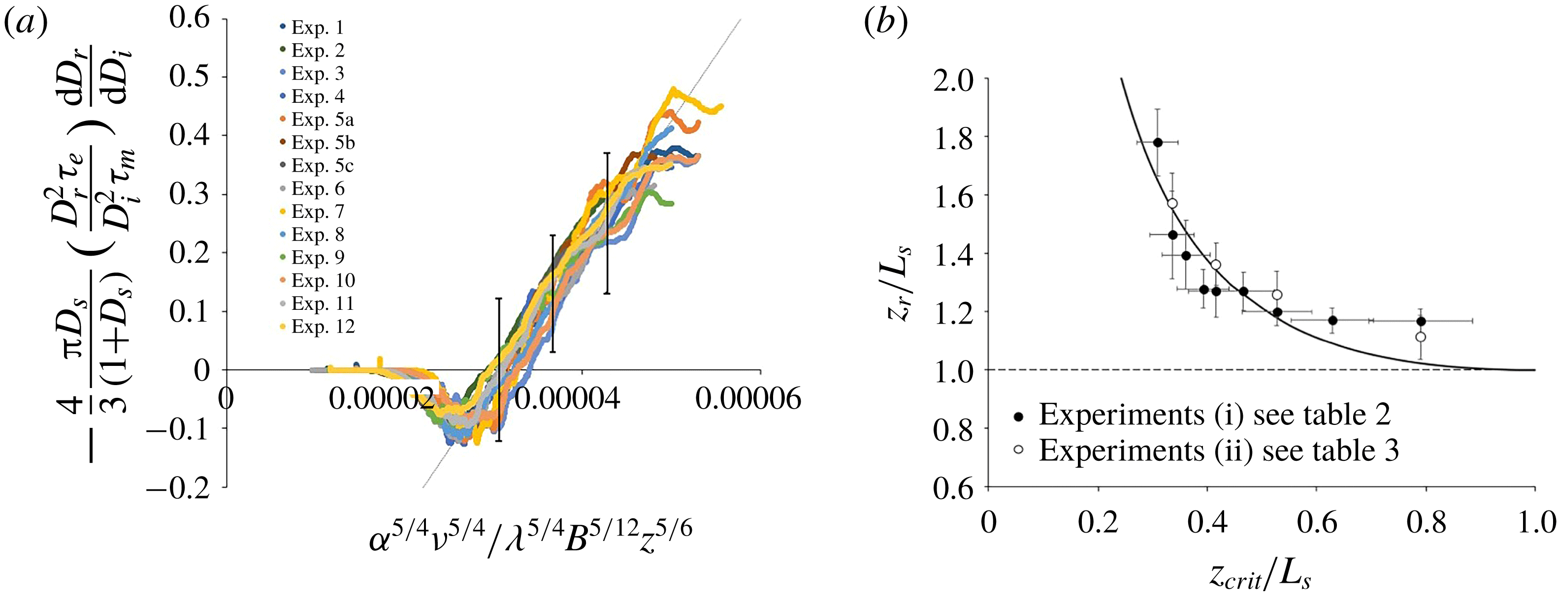
Equation (5.32) and the results of the experiments described in §§ 3.1 and 3.2 are used to plot figure 11(a). It is seen that for
 $z_{crit}<z<z_{r}$
, the data collected during a number of different experiments collapse onto a line: by measuring the slope of this line, we estimate that
 $\unicode[STIX]{x1D6FD}Sc_{b}^{-3/2}(\ln Sc_{b})^{-2}\approx \left(2.0\pm 0.14\right)\times 10^{4}$
in our experiments; given the values of
 $Sc_{b}$
listed in tables 2 and 3, we then obtain
 $\unicode[STIX]{x1D6FD}\approx \left(8.95\pm 0.63\right)\times 10^{9}$
. It should be noted that, since (5.30)–(5.32) are based on the approximation that the volume of each parcel of fluid in the plume is proportional to the third power of
 $D$
and involve a derivative of the experimental measurements, we should not expect the collapse of the experimental results depicted in figure 11(a) to be perfect. Furthermore, (5.32) only applies to the region of the flow in which the mixing of the entrained fluid is incomplete, and is not applicable to the near-source region,
 $0<z<z_{crit}$
(see (5.24)). For this reason, we do not expect the vertical intercepts of the sloping lines in figure 11(a) to be equal to zero, and a dimensionless constant
 $c_{1}$
has been added to (5.33) accordingly. Since both the buoyancy flux
 $B$
(
 $\text{m}^{4}~\text{s}^{-3}$
) and the viscosity
 $\unicode[STIX]{x1D708}$
(
 $\text{m}^{2}~\text{s}^{-1}$
) were typically of the order of
 $10^{-6}$
in our experiments (see tables 2 and 3), we calculate that
 $z_{crit}\approx 0.10$
m in our experiments (5.25). This implies that
 $z_{crit}<L_{s}$
in most of the experiments listed in tables 2 and 3.
The estimated value of
 $\unicode[STIX]{x1D6FD}$
and (5.29) are used to calculate how the ratio
 $z_{r}/L_{s}$
changes as a function of
 $z_{crit}/L_{s}$
. In figure 11(b), the prediction of the model (solid line) is compared with the results of the experiments (symbols). For each experiment, we detect the distance from the virtual source at which the time-averaged light attenuation produced by the reactive plume (red line in figure 5
e) is 20 times smaller than that produced by the inert plume (black line in figure 5
e). At this particular threshold, the light attenuation produced by the reactive plume is too faint to be perceived with the naked eye, but it can be captured and quantified using the image analysis technique described in § 2. At larger distances from the source, however, our experimental technique becomes less accurate as the signal-to-noise ratio of the light attenuation produced by the reactive plume decreases. For each experiment, the measured distance is scaled by the stoichiometric length scale
 $L_{s}$
, and the result is plotted in figure 11(b) using an open or filled circle. It is seen that our experimental results compare well with the predictions of the model, with discrepancies of the order of 5 %–10 % approximately.
5.3.5 Light attenuation profiles
The ratio between the critical distance
 $z_{crit}$
and the stoichiometric length scale
 $L_{s}$
can be given as a function of the entrainment, mixing and stoichiometric time scales (see table 5):
 $$\begin{eqnarray}\frac{z_{crit}}{L_{s}}=\frac{\unicode[STIX]{x1D6FE}^{6/5}\unicode[STIX]{x1D70F}_{m}^{3}}{\unicode[STIX]{x1D70F}_{s}\unicode[STIX]{x1D70F}_{e}^{2}},\end{eqnarray}$$
in which
 $$\begin{eqnarray}\unicode[STIX]{x1D6FE}=\frac{\unicode[STIX]{x1D6FD}}{Sc_{b}^{3/2}(\ln Sc_{b})^{9/2}}\end{eqnarray}$$
is used for convenience. Using (5.27) and (5.33), the fraction of the supplied chemicals that are still reactive at a distance
 $z$
below the source,
 $R$
, is given as a function of the time
 $t$
required for the plume fluid to flow from the source to
 $z$
, as
 $$\begin{eqnarray}R(t)=\left\{\begin{array}{@{}l@{}}\displaystyle 1-\left({\displaystyle \frac{t}{\unicode[STIX]{x1D70F}_{s}}}\right)^{5/3},\quad 0<{\displaystyle \frac{t}{\unicode[STIX]{x1D70F}_{s}}}<{\displaystyle \frac{\unicode[STIX]{x1D6FE}^{6/5}\unicode[STIX]{x1D70F}_{m}^{3}}{\unicode[STIX]{x1D70F}_{s}\unicode[STIX]{x1D70F}_{e}^{2}}},\\ \displaystyle 1+{\displaystyle \frac{\unicode[STIX]{x1D6FE}^{2}\unicode[STIX]{x1D70F}_{m}^{5}}{\unicode[STIX]{x1D70F}_{s}^{5/3}\unicode[STIX]{x1D70F}_{e}^{10/3}}}-{\displaystyle \frac{2\unicode[STIX]{x1D6FE}\unicode[STIX]{x1D70F}_{m}^{5/2}}{\unicode[STIX]{x1D70F}_{s}^{5/6}\unicode[STIX]{x1D70F}_{e}^{5/3}}}\left({\displaystyle \frac{t}{\unicode[STIX]{x1D70F}_{s}}}\right)^{5/6},\quad {\displaystyle \frac{\unicode[STIX]{x1D6FE}^{6/5}\unicode[STIX]{x1D70F}_{m}^{3}}{\unicode[STIX]{x1D70F}_{s}\unicode[STIX]{x1D70F}_{e}^{2}}}<{\displaystyle \frac{t}{\unicode[STIX]{x1D70F}_{s}}}<{\displaystyle \frac{t_{r}}{\unicode[STIX]{x1D70F}_{s}}}.\end{array}\right.\end{eqnarray}$$
In (5.35),
 $t_{r}$
denotes the time required for the plume fluid to flow from the source to the level at which the instantaneous chemical reaction reaches completion,
 $z_{r}$
. Using a combination of (5.29) and (5.33), we calculate that this time lapse is given by
 $$\begin{eqnarray}\frac{t_{r}}{\unicode[STIX]{x1D70F}_{s}}=\left(\frac{\unicode[STIX]{x1D6FE}^{2}\unicode[STIX]{x1D70F}_{m}^{5}+\unicode[STIX]{x1D70F}_{s}^{5/3}\unicode[STIX]{x1D70F}_{e}^{10/3}}{2\unicode[STIX]{x1D6FE}\unicode[STIX]{x1D70F}_{m}^{5/2}\unicode[STIX]{x1D70F}_{s}^{5/6}\unicode[STIX]{x1D70F}_{e}^{5/3}}\right)^{6/5}.\end{eqnarray}$$
Fraction of the supplied chemicals that are still reactive in the plume,
 $R$
, as a function of time. Equations (5.18) and (5.35) are used to plot the model predictions for slow and fast reaction experiments (red and black lines, respectively). Symbols are used to illustrate the ratio between the time-averaged mean light attenuation produced by a reactive plume and that produced by an inert plume as measured during our experiments. On the horizontal axis, time is scaled by the stoichiometric time scale
 $\unicode[STIX]{x1D70F}_{s}$
given by (5.14).

Equation (5.35) is used to plot the black solid curve in figure 12. This line illustrates the theoretical prediction of the minimum fraction of reactive chemicals in the plume fluid,
 $R(t)$
, in the case that the chemical reaction is instantaneous and mixing is complete (
 $z_{crit}\geqslant L_{s}$
). This theoretical prediction is compared with the results of the fast reaction experiments (black and grey symbols, see tables 2 and 3). Each symbol in figure 12 illustrates the ratio between the time- and depth-averaged mean intensity of light attenuation produced by a reactive plume and that produced by the associated inert plume at a given height in the tank during an experiment. It is seen that, at small distances and times from the source (
 $t/\unicode[STIX]{x1D70F}_{s}<0.3{-}0.5$
and
 $R>0.7{-}0.8$
approximately), there is a relatively good agreement between the results of the experiments and the model prediction illustrated by the black solid curve. However, for
 $t/\unicode[STIX]{x1D70F}_{s}>0.5$
and
 $R<0.7$
approximately, the experimental results deviate from the black solid curve: in this region, the mean concentration of reactive chemicals in the plume fluid in our experiments is larger than that predicted by (5.35) as a result of incomplete mixing. Given that
 $z_{crit}/L_{s}>0.30$
in all of our fast reaction experiments (see figure 11
b), we use (5.35) to plot the dashed black curve in figure 12, which illustrates the theoretical prediction for
 $R(t)$
in the case
 $z_{crit}/L_{s}=0.30$
. Figure 12 shows that most of the data points collected during the fast reaction experiments lie between the two black curves, as expected.
In figure 12, the model predictions and the results of our slow reaction experiments are plotted for comparison. For
 $\unicode[STIX]{x1D70F}_{s}/\unicode[STIX]{x1D70F}_{r}\ll 1$
, we assume that the chemical species are well mixed within the plume fluid (see § 2); this in turn implies that
 $R$
equals the ratio between the concentration of dye in the reactive plume fluid and that in the inert plume fluid,
 $C_{b,reaction}/C_{b,inert}$
. We therefore use (5.18) to plot the solid and the dashed red curves in figure 12: these lines illustrate the two bounding profiles associated with the maximum and minimum concentrations of reactants in the ambient fluid in our experiments. It is seen that all experimental results (yellow and red symbols, experiments 17–21 in table 4) lie between these two bounding profiles, as expected. Figure 12 shows that in the slow reaction experiments, a considerable amount of time is required for the consumption of the chemical species in the plume, and most of the reaction develops at times larger than
 $\unicode[STIX]{x1D70F}_{s}$
, i.e. at distances larger than
 $L_{s}$
below the source. Furthermore, as the concentration of the supplied chemical species in the plume fluid decreases, the rate of the pseudo-first-order reaction also decreases. As indicated by (5.18), the pseudo-first-order reaction only reaches completion when
 $t\rightarrow \infty$
.
6 Conclusions
We have explored the behaviour of a reactive turbulent plume in the two limiting cases of (i) a slow reaction, which develops on a time scale longer than the time required for the entrained fluid to be mixed in the plume, and (ii) a faster reaction, which develops in a fraction of the mixing time. New experiments have been carried out using light attenuation techniques for selected acid–base and redox chemical reactions. The measurements show that, when the reaction is sufficiently slow, the entrained and source chemicals are rapidly mixed, and the reaction takes place throughout the entire volume of each eddy in the plume. However, faster reactions develop only at the periphery of each eddy, where the plume and the entrained fluids are mixed locally at the Batchelor scale (see figure 8 b). The mixture of fluids in this border region becomes rapidly neutralised, while the concentration of reactants in the core of the parcel is not affected by the reaction.
Motivated by the experimental results, we have developed a model that quantifies the fraction of the entrained fluid that reacts with the source fluid in the plume. Our model indicates that the volume flux of entrained fluid increases with distance from the source (see (5.23)), while the volume flux of fluid that is mixed within the plume at the Batchelor scale decreases with distance from the source (see (5.22)). Hence, a critical level
 $z_{crit}$
exists at which the two fluxes are equal (see (5.25)). In the region spanning between the plume source and this critical level,
 $z<z_{crit}$
, the entire flux of entrained fluid is mixed locally and reacts within the plume, and so the progress of the reaction is limited by entrainment. However, at larger distances from the source,
 $z>z_{crit}$
, only a fraction of the entrained fluid is mixed locally within the plume, and the progress of the reaction is limited by incomplete mixing. The experimental measurements of the average size of the plume eddies,
 $D_{i}$
, and of the average size of the parcels of reactive fluid in the plume,
 $D_{r}$
(see figure 7), have enabled us to quantify
 $z_{crit}$
as a function of dimensionless coefficient
 $\unicode[STIX]{x1D6FD}$
(see (5.25) and figure 11
a). As a result of the non-uniform mixing of the fluids in the plume, the distance from the source at which an instantaneous reaction is complete,
 $z_{r}$
, is larger than that predicted using the classical plume theory,
 $L_{s}$
. Both the longitudinal concentration profile of source chemical in the plume and the ratio
 $z_{r}/L_{s}$
are shown to depend on
 $(z_{crit}/L_{s})^{5/6}$
.
Appendix A. Turbulent properties of the flow
A.1 Source Reynolds number, entrainment coefficient
In each of our experiments, a turbulent, negatively buoyant plume was formed by supplying relatively dense, dyed fluid through the nozzle located at the top of the tank (see figure 1). Based on the known source volume flux
 $Q_{0}$
and nozzle radius
 $r_{0}$
(see tables 2–4), we estimate that the mean flow speed at the nozzle was
 $u_{0}=0.45$
m s
 $^{-1}$
in experiments 1–16 (tables 2 and 3) and
 $u_{0}=0.88$
m s
 $^{-1}$
in experiments 17–21 (table 4). We then estimate the associated Reynolds number to be
 $Re_{0}=1061$
(see tables 2–4). It is seen that our experiments were conducted under
 $Re$
conditions comparable to or exceeding those of many published studies on turbulent plumes, including: George, Alpert & Tamanini (Reference George, Alpert and Tamanini1977),
 $Re_{0}=870$
; Papanicolau & List (Reference Papanicolau and List1988),
 $Re_{0}=600$
; Woods & Caulfield (Reference Woods and Caulfield1992),
 $Re_{0}\approx 200$
(where the authors note that the flow was laminar at the source, but became fully turbulent 2–3 cm below the source); and Ulpre et al. (Reference Ulpre, Eames and Greig2013),
 $Re_{0}=399$
.
The time-averaged, mean velocity of the fluid descending along the plume centreline at larger distances from the source was measured in a number of experiments using the procedure described in § 2.2. Figure 4(b) shows that the measured velocities decrease with distance from the source in agreement with the theoretical prediction for fully turbulent plumes (Morton et al. Reference Morton, Taylor and Turner1956).
As described in § 2.2, two filling-box experiments were performed in the tank to quantify the entrainment coefficient
 $\unicode[STIX]{x1D6FC}$
(cf. Linden et al.
Reference Linden, Lane-Serff and Smeed1990). During these experiments, the tank was initially filled with fresh water and relatively dense, dyed inert fluid was supplied through the nozzle. The supplied fluid descended through the tank in the form of a plume, and eventually accumulated at its base. As a result, the tank became stratified, with a sharp interface separating the clear fluid at the top of the tank from the dyed fluid underneath. During each filling-box experiment, we measured the rising speed of this interface, and used the collected data to estimate the volume flux in the plume as a function of distance from the source,
 $Q(z)$
. In both experiments, we found that
 $Q(z)\sim z^{5/3}$
, as predicted by the classical theory of turbulent plumes (Morton et al.
Reference Morton, Taylor and Turner1956). We then used the measured flow rates to estimate
 $\unicode[STIX]{x1D6FC}=0.10\pm 0.02$
(see § 2.2), which is consistent with the literature for turbulent plumes.
The results of the filling-box experiments also enabled us to quantify the time scale for the experimental tank to become contaminated during an experiment. Given that the buoyancy flux
 $B$
in our experiments was typically of the order of
 $10^{-6}~\text{m}^{4}~\text{s}^{-3}$
(see tables 2–4), and given that the height of the tank was
 $H=0.7$
m (see figure 1), the maximum volume flux in the plume at base of the tank was of the order of
 $Q_{max}\approx 5\times 10^{-5}~\text{m}^{3}~\text{s}^{-1}$
(see (5.1)). Since the volume of ambient fluid in the tank was of the order of 0.12 m
 $^{3}$
, we estimate the filling time scale to be larger than 2400 s (40 min) approximately. As discussed in § 2.1, each of our experiments typically lasted 2.5–3 min. We therefore conclude that the impact of environmental stratification was negligible during our experiments.
A.2 Impacts of source momentum flux
As discussed in § 2.1, the source plume fluid was supplied to the experimental tank using a peristaltic pump; hence, the source volume and momentum fluxes were finite. In order to estimate the impacts of the source conditions, for each experiment listed in tables 2–4, we calculate the Morton number
 $\unicode[STIX]{x1D6E4}_{0}$
(Hunt & van den Bremer Reference Hunt and van den Bremer2011):
 $$\begin{eqnarray}\unicode[STIX]{x1D6E4}_{0}=\frac{5BQ_{0}^{2}}{8\unicode[STIX]{x1D6FC}\unicode[STIX]{x03C0}^{1/2}M_{0}^{5/2}}.\end{eqnarray}$$
Tables 2–4 show that in our experiments
 $\unicode[STIX]{x1D6E4}_{0}$
was of the order of
 $10^{-2}$
; this indicates that our plumes were forced at the source, and that at small distances from the source the momentum
 $M(z)$
was larger than that of a pure plume. As a result, the descending flow behaves like a buoyant jet in the near-source region. Following Hunt & Kaye (Reference Hunt and Kaye2001), we calculate the length scale
 $L_{M_{0}}$
for the region in which the flow was affected by the initial momentum:
 $$\begin{eqnarray}L_{M_{0}}=2^{-3/2}\unicode[STIX]{x1D6FC}^{-1/2}M_{0}^{3/4}B^{-1/2}.\end{eqnarray}$$
Tables 2–4 show that
 $L_{M_{0}}\ll L_{s}$
in all our experiments. We also solve the classical plume equations for the mass flux
 $Q(z)=\unicode[STIX]{x03C0}q(z)$
, momentum flux
 $M(z)=\unicode[STIX]{x03C0}m(z)$
and buoyancy flux
 $B(z)=\unicode[STIX]{x03C0}b(z)$
integrated across each horizontal plane in the plume (cf. Turner Reference Turner1973):
 $$\begin{eqnarray}\frac{\text{d}q}{\text{d}z}=2\unicode[STIX]{x1D6FC}m^{1/2},\quad \frac{\text{d}m}{\text{d}z}=bq/m,\quad \frac{\text{d}b}{\text{d}z}=-N^{2}q=0,\end{eqnarray}$$
and compare the numerical solution for
 $q(z)$
with the analytical solution for a pure plume originating at the virtual origin
 $z_{0}$
(see (5.1)). We obtain that at distances 0.25–0.30 m below the source, the volume flux in the plume estimated using the analytical solution given in § 5.1.1 is in good agreement with that estimated using the system of (A 3), with errors of the order of 3 %–6 %. This confirms that, whereas the source momentum flux
 $M_{0}$
affected the flow in the near-source region, the entrainment of ambient fluid into the plume was governed by buoyancy beyond this region. Hence, our measurements of the critical distance from the source at which the chemical reaction reaches completion were only marginally affected by the initial momentum of the flow, and the errors associated with the source conditions were smaller than those associated with the image analysis technique (see § 2.2).
Appendix B. Ranges of chemical concentrations and buoyancy fluxes used in the experiments
The range of conditions used in our fast reaction experiments is given in tables 2 and 3. It is seen that a number of different experiments were conducted, using plumes with: (i) different buoyancy fluxes and (ii) different concentrations of chemicals. In a first group of fast reaction experiments (1–10 and 13–16 in tables 2 and 3), the source buoyancy flux
 $B$
was fixed, while the ratio between the concentration of the chemical species in the plume and in the ambient fluid,
 $C_{b}^{0}/Ca$
, was changed systematically. Since the chemical reactions used in these experiments did not affect
 $B$
, the plume radius, speed and density were identical in this set of experiments. Tables 2 and 3 show that the critical stoichiometric dilution
 $D_{s}$
ranged between 15 and 129 as a result of the different concentrations of chemical species used in the experiments (see (5.12)); this in turn led to the stoichiometric length scale
 $L_{s}$
varying between 10 and 38 cm in different experiments (see (5.13)). As discussed in § 5.3, owing to incomplete mixing of the fluid in the plume, the distance from the source at which the fast reaction reached completion was up to 1.6–1.8 times larger than
 $L_{s}$
in our experiments (see figure 11
b), leading to
 $z_{r}+z_{0}\approx 60{-}65$
cm. The investigation of the impact of a wider range of chemical concentrations would have been difficult in the laboratory. Lower concentrations of reactants in the plume fluid would have resulted in
 $D_{s}<10{-}15$
and
 $L_{s}<10$
cm (see table 2): in this case, the supplied chemical species would have been neutralised at small distances from the nozzle, where the plume flow may be somehow affected by the initial momentum and source conditions (see appendix A). Higher concentrations of supplied reactant would result in
 $D_{s}>130{-}150$
, and thus the reaction would have reached completion at large distances from the source, which are incompatible with the vertical dimension of the experimental tank.
Equations (5.21) and (5.25) indicate that there is one key parameter in the model,
 $z_{crit}$
, which varies as a function of the buoyancy flux, and is not affected by the concentration of chemical species in the plume. Hence, two additional experiments (11 and 12 in table 2) were performed using the same chemical properties as in experiment 4, but different buoyancy fluxes. In order to obtain different values of
 $B$
, either different densities of the plume fluid,
 $g_{0}^{\prime }$
, or different volumetric flow rates,
 $Q_{0}$
, could have been used at the plume source. For the source conditions of experiments 11 and 12 to be as close as possible to those of the other experiments, we chose only to let
 $g_{0}^{\prime }$
vary, and kept the source volume flux
 $Q_{0}$
fixed (see table 2). This resulted in
 $Re_{0}$
,
 $\unicode[STIX]{x1D6E4}_{0}$
and
 $L_{M_{0}}$
being the same across the different experiments. In order to increase the source density of the plume fluid, inert NaCl was added to the fluid as discussed in § 3.1. The ratio between the largest and the smallest values of
 $g_{0}^{\prime }$
that we could achieve was 4. Since
 $z_{crit}\sim B^{-1/2}$
(see (5.21) and (5.25)), this resulted in the critical distance
 $z_{crit}$
varying by a factor of 2 among the different experiments. The impacts of such a variation on the profile of concentration of chemical species in the plume were large enough that they could be measured using our experimental procedure.