2.1 Resource description framework (RDF)

Resource Description Framework (RDF) is a W3C recommendation for the notation of metadata on the World Wide Web (WWW) (RDF). The basic idea of RDF is a triple model, where:

1. • Anything is called ‘resource’. A resource (identified by International Resource Identifier IRI) has ‘properties’, and these properties have values, which may be literal values (e.g. string or integer) or other resources.

2. • The relationships among resources, properties, and values can be expressed by ‘statements’, which have the triple structure:

It is usually abbreviated as <s p o>. The subject or s identifies the thing that the statement is about, the predicate or p identifies the property or characteristic of the subject, and the object or o identifies the value of the property.

There are several kinds of syntax to describe RDF data such as Turtle family of RDF languages, JSON-LD (JSON-based RDF syntax), RDFa (for HTML and XML embedding), RDF/XML (XML syntax for RDF) RDF. Here is an example of an RDF triple with Turtle syntax to describe a statement ‘Baron Way Building is located in Amsterdam’:

Further, RDF Schema (RDFS) (RDF) can enrich and define semantic characteristics of RDF data. RDFS uses class (denoted by the syntactic form rdfs:Class) to specify categories that can be used to classify resources. The relation between an instance and its class is stated through the property type (rdf:type). With RDFS, one can create hierarchies of classes and subclasses (rdfs:subClassOf) and of properties and sub-properties (rdfs:subPropertyOf). Type restrictions on the subjects and objects of particular triples can be defined through domain (rdfs:domain) and range (rdfs:range) restrictions. Also, a set of entailment rules are defined for RDF and RDFS. Conceptually, these rules specify that an additional triple can be added to an RDF graph if the graph contains triples of a specific pattern. For example, if two triples (x, rdfs:subClassOf, y) and (y, rdfs:subClassOf, z), one can infer that (x, rdfs:subClassOf, z). Further, OWL (Web Ontology Language, 2012) adds more vocabulary than RDFS for describing properties and classes.

For example, one can state that the IRI http://www.example.org/friendOf can be used as a property and that the subjects and objects of http://www.example.org/friendOf triples must be resources of class http://www.example.org/Person . Such example can be expressed by the following triples (where http://www.example.org/ is denoted by the prefixe ‘ex’):

For indexing RDF data, the query language (SPARQL, 2013) has been the standardized query language for RDF. SPARQL is based on matching graph patterns. Most forms of SPARQL query contain a set of triple patterns called a basic graph pattern. Triple patterns are like RDF triples except that each of the subject, predicate, and object may be a variable. A basic graph pattern matches a subgraph of the RDF data when RDF terms from that subgraph may be substituted for the variables and the result is RDF graph equivalent to the subgraph. The variable bindings can be restricted through filters, which are essentially functions returning a Boolean. SPARQL specifies a number of built-in filter functions, such as regex or the usual comparison operators (>, $!=$ , …), and also allows additional filter functions that are identified by an IRI. Moreover, SPARQL also contains capabilities for querying required and optional graph patterns along with their conjunctions and disjunctions.

Please refer to (RDF) and (SPARQL, 2013) for more detailed introduction about RDF, RDFS, and SPARQL.

2.2 Spatial and spatiotemporal data

Here, we first recall several basic notions frequently mentioned in the later text. Raster and vector are two very different but common data representations, which are used to store geospatial data (Athanasiou et al., Reference Athanasiou, Bezati, Giannopoulos, Patoumpas and Skoutas2012). Vector data use x and y coordinates to define the locations of points, lines, and areas, or polygons, which correspond to physical entities in the real world, such as roads, parcels. Raster data use a matrix of square areas to define where physical entities are located, and such squares are also named as pixels, cells, and grids.

Moreover, features and geometries are two crucial geospatial concepts (ISO, 2004; Athanasiou et al., Reference Athanasiou, Bezati, Giannopoulos, Patoumpas and Skoutas2012):

1. • A feature is an abstraction of real-world phenomena (e.g. a Station, a Road, or Pretty much anything), which has some spatial location. A feature can occur as a type or an instance. Feature type or feature instance will be used when only one is meant. A feature type is a class of features having common characteristics. A feature instance is a single occurrence of the feature type and represented as an object in a dataset.

2. • A geometry can be any geometric shape, typically a point, a polyline or, a polygon, as well as several more complex variants (e.g. a polygon with holes). This geometry serves as the spatial location of a given feature using coordinates. Depending on the desired resolution and purpose of use, the location may be defined as one or more geometric shapes. For example, a train station may take the shape of a point (e.g. its centroid to be included in a city map), or a region (in a detailed map of more accuracy), and perhaps even a line (if only its boundary is important). A geometry can be a homogeneous collection (e.g. a multipoint denoting a set of measurements) or a heterogeneous one (e.g. a polygon along with its centroid can be considered as the representation of a region).

Note that every geometry must be always georeferenced at a well-defined system of coordinates (spatial reference systems SRS or coordinate reference systems CRS). A CRS defines how to relate the coordinates of a geometric object to real locations on the surface of Earth. An important part of the metadata associated with a geometry is its CRS. The elements of a coordinate reference system provide context for the coordinates that define a geometry in order to accurately describe their position and establish relationships between sets of coordinates. There are four parts that make up a CRS: a coordinate system, an ellipsoid, a datum, and a projection (Battle & Kolas, Reference Battle and Kolas2012; OGC GeoSPARQL 2012). Various types of CRS exist, for example, geographic CRS (latitude–longitude and optionally ellipsoidal height, e.g the World Geodetic System 1984-WGS84 is a well-known geographic CRS), 3-dimensional cartesian geocentric CRS (X, Y, Z), and projected (X, Y) (Koubarakis et al., Reference Koubarakis, Kyzirakos and Nikolaou2012). One common source of well-defined coordinate reference systems is the European Petroleum Survey Group (EPSG), where each CRS is assigned a unique identifier.

Spatial data types (Schneider, Reference Schneider2009) or geometric data types provide a fundamental abstraction for modeling the geometric structure of objects in space as well as their relations. One speaks of spatial objects as values of spatial data types. The familiar spatial data types include 2-dimensional data types for points (e.g. representing the location of a building), lines (e.g. describing the ramifications of the Nile Delta), regions (e.g. depicting air-polluted zones), spatial networks (e.g. representing the routes of the Metro), and spatial partitions (e.g. describing the states of a country and their exclusively given topological relationships of adjacency or disjointedness) as well as 3-dimensional data types for surfaces (e.g. modeling the shape of landscapes) or volumes (e.g. representing urban areas).

Spatial information is usually represented by the literals of the spatial data types (Smeros & Koubarakis, Reference Smeros and Koubarakis2016). WKT (Well-Known Text) (ISO 2004) (OGCSF) and GML (Geography Markup Language) (GML) are universally used for the serialization of spatial literals. WKT is an OGC (Open Geospatial Consortium) standard for the representation of vector geometry objects, CRSs (Coordinate Reference Systems), and transformation rules between different CRSs. It is also the ISO 19125-1 standard (ISO 2004), which deals with the representation and manipulation of simple features (a simple feature is a feature with all its spatial attributes described piecewise by straight line or planar interpolation between sets of points). As mentioned in Koubarakis et al. (Reference Koubarakis, Kyzirakos and Nikolaou2012), geometries in WKT are restricted to 0-, 1-, and 2-dimensional geometric objects that exist in 2-, 3-, or 4-dimensional coordinate space (i.e. $\mathbb{R}^{2}$ , $\mathbb{R}^{3}$ , or $\mathbb{R}^{4}$ ). Geometries that exsit in $\mathbb{R}^{2}$ consists of points with coordinates x and y, for example, POINT(1, 2). Geometries that exsit in $\mathbb{R}^{3}$ consists of points with coordinates x, y, and z or x, y, and m, where m is a measurement. For instance, POINT(37.96, 23.71, 27) denotes the temperature (measured in Celsius degree) of a city. Geometries that exsit in $\mathbb{R}^{4}$ haves points with coordinates x, y, z, and m, for example, POINT(1, 1, 2, 27). GML, developed by OGC as well, is the most common XML-based encoding standard for the representation of geospatial data, and provides XML schemas for defining a variety of concepts that are of use in Geography.

Further, the common spatial relations include topological, directional, and metric relations (Papadias & Theodoridis, Reference Papadias and Theodoridis1997; Chbeir et al., Reference Chbeir, Amghar and Flory2003). Topological relations describe concepts of neighborhood, incidence, and overlap and stay invariant under transformations such as scaling and rotation, and can be used to check the relative position of spatial objects to each other like overlap, meet, disjoint, or inside. RCC-8 model (Randell et al., Reference Randell, Cui and Cohn1992) and Egenhofer’s model (Egenhofer & Herring, Reference Egenhofer and Herring1991) are the widely used models for analyzing topological relations. Direction relations give a qualitative support to evaluate the relative position of spatial objects like north or southeast. Metric relations measure the distance between spatial objects like far or nearby. Moreover, there is a set of spatial operations that can be applied on spatial data (Gür et al., Reference Gür and Pedersen2018), including spatial aggregation, topological relations as mentioned above, and numeric operations. The spatial aggregation operators aggregate two or more spatial objects and return a new spatial object such as Union, Intersection, ConvexHull, and Minimum Bounding Rectangle (MBR). The numeric operations take one or more spatial objects and return a numeric value such as Perimeter, Area, NoOfInteriorRings, Distance, HaversineDistance, and NoOfGeometries.

Spatiotemporal data types (Schneider, Reference Schneider2009) are used to represent the temporal evolution of spatial objects over time, for example, as in the case of moving objects. Different temporal types are classified including user-defined time (which has no special semantics, e.g January 1, 1963 when John has his birthday), valid time (which is the time a fact is true in the application domain, e.g. the time 2000–2012 when John is a professor), transaction time (which is the time when a fact is current in the database, e.g. the system time that gives the exact period when the tuple representing that John is a professor from 2000 to 2012 is current in the database), combination of transaction time and valid time (Snodgrass & Ahn 1985; Date et al., Reference Date, Darwen and Lorentzos2002). These evolutions can be discrete or continuous. The common spatiotemporal data types include moving point (e.g. recording the route of a cell phone user), moving line (e.g. representing the boundary of a tsunami), and moving region (e.g. describing the motion of an air polluted cloud). Operations on spatiotemporal data types comprise, for instance, the spatiotemporal intersection, union, and difference of moving objects, the computation of the trajectory of a moving point as a line object, the determination of the location of a moving object at a particular time, the calculation of a moving object during a given set of intervals, and the test whether a moving point enters or crosses a moving region. Moreover, with the demand of spatiotemporal applications, a lot of work have been made to modeling, storing, and querying spatiotemporal data (Pelekis et al., Reference Pelekis, Theodoulidis and Kopanakis2004; Nandal, Reference Nandal2013; Rathee & Yadav, Reference Rathee and Yadav2013).

3.1 Spatial RDF representation

There have been several attempts for representing and managing geospatial data in RDF, and establishing geospatial RDF standard. As also mentioned in Athanasiou et al. (Reference Athanasiou, Bezati, Giannopoulos, Patoumpas and Skoutas2012) and Patroumpas et al. (Reference Patroumpas, Alexakis and Giannopoulos2014), early work including the W3C Basic Geo Vocabulary (W3C GEO 2003), which enabled the representation of points in WGS84 (World Geodetic System, 1984, the most common CRS for spatial data on the web), and GeoRDF as an RDF compatible profile for geographic information (points, lines and polygons). In particular, the OGC GeoSPARQL standard (Battle & Kolas, Reference Battle and Kolas2012; OGC GeoSPARQL 2012) supports representing and querying geospatial data. Table 1 first summarizes and compares the spatial RDF representation forms.

Table 1.

Summarization and comparison of spatial RDF representation

(1) GeoSPARQL (Battle & Kolas, Reference Battle and Kolas2012 ; OGC GeoSPARQL, 2012)

The OGC GeoSPARQL standard supports representing and querying geospatial data on the Semantic Web. GeoSPARQL defines a vocabulary for representing geospatial data in RDF, and it defines an extension to the SPARQL query language for processing geospatial data.

In detail, by following a modular design, GeoSPARQL comprises several different components for representing geospatial data in RDF:

1. • Core. Defines top-level RDFS classes for spatial objects. Two main classes are defined: geo:SpatialObject and geo:Feature, where geo is the XML namespace prefix of http://www.opengis.net/ont/geosparql$\#$. The geo:SpatialObject represents everything that can have a spatial representation. The geo:Feature represents the top-level feature type and is superclass of all feature types. Note that the geo:Feature is subclass of the geo:SpatialObject and is equivalent to the class GFI $\_$ Feature (ISO 19156) (where GFI $\_$ Feature represents the set of all classes which are feature types and is an instance of the $\ll metaclass\gg$ GF $\_$ FeatureType defined in ISO 19109 Rules for application schema (ISO 2005)).

2. • Topology Vocabulary Extension (relation $\_$ family). Defines RDF properties for asserting and querying topological relations between spatial objects. Such component is parameterized so that different families of topological relations (such as Simple Features relations (ISO 2004; OGCSF), RCC-8 relations (Randell et al., Reference Randell, Cui and Cohn1992), and Egenhofer’s Nine-Intersection relations (Egenhofer & Herring, Reference Egenhofer and Herring1991)) may be used. For example, the RDF properties geo:rcc8eq, geo:rcc8dc, geo:rcc8ec, geo:rcc8po, geo:rcc8tppi, geo:rcc8tpp, geo:rcc8ntpp, geo:rcc8ntppi can be used for representing the RCC-8 topological relations. Note that the OGC Simple Features relations build on the DE-9IM (Dimensionally Extended Nine-Intersection Model (Clementini & Di Felice, Reference Clementini and Di Felice1995)) and offer the relations: Equals, Disjoint, Intersects, Touches, Crosses, Within, Contains, Overlaps, and Relate.

3. • Geometry Extension (serialization, version). Defines RDFS data types for serializing geometry data, geometry-related RDF properties, and non-topological spatial query functions for geometry objects. The serialization specifies the serialization standard (e.g. WKT and GML as mentioned in Section 2.2) to use when generating geometry literals and also the supported geometry types. The version specifies the version of the serialization format used. Note that the serialization chosen strongly affects the geometry conceptualization. The WKT serialization aligns the geometry types with ISO 19125-1 Simple Features (ISO 2004). The GML serialization aligns the geometry types with ISO 19107 Spatial Schema (ISO 2003), which is a much wider range than the simple features allowed in WKT, including a lot of less commonly used types.

   In detail, a single root geometry class geo:Geometry is defined, which represents the top-level geometry type and is superclass of all geometry types. The class geo:Geometry is equivalent to the UML class GM $\_$ Object defined in ISO 19107 Spatial Schema (ISO 2003). Also, the class geo:Geometry is subclass of the geo:SpatialObject and is disjoint with the class geo:Feature. Moreover, two properties are defined for associating geometries with features. A property geo:hasGeometry is used to link a feature with a geometry that represents its spatial extent. A given feature may have many associated geometries. Also, a subproperty of the geo:hasGeometry, called geo:hasDefaultGeometry, is used to link a feature with its default geometry. In addition, several properties for geo:Geometry are defined for describing geometry metadata, such as geo:dimension, geo:coordinateDimension, geo:spatialDimension, geo:isEmpty, geo:isSimple, geo:hasSerialization, where the geo:hasSerialization property is used to connect a geometry with its text-based serialization (e.g. its WKT serialization). Further, an RDFS datatype geo:wktLiteral is defined for representing geometry data in RDF based on WKT as defined by ISO 19125-1 Simple Features (ISO 2004). For example, ‘Point(-83.38 33.95)’geo:wktLiteral encodes a point geometry using the default WGS 84 (World Geodetic System 1984, the most common CRS for spatial data on the web) geodetic longitude-latitude spatial reference system for Simple Features 1.0. At the same time, a subproperty of the geo:hasSerialization, called geo:asWKT is defined to link a geometry with its WKT serialization. Similarly, an RDFS datatype geo:gmlLiteral is defined for representing geometry data in RDF based on GML as defined by Geography Markup Language Encoding Standard OGC, and a subproperty of the geo:hasSerialization, called geo:asGML is defined to link a geometry with its GML serialization.

4. • Geometry Topology Extension (relation $\_$ family, serialization, version). Defines topological query functions, which will be introduced in the subsequent query section.

5. • RDFS Entailment Extension (relation $\_$ family, serialization, version). Defines a mechanism for matching implicit RDF triples that are derived based on RDF and RDFS semantics. For example, the ISO 19125-1 Simple Features (ISO 2004) specification presents a geometry class hierarchy. It is straightforward to represent this class hierarchy in RDFS. That is, the hierarchy relationship between Polygon and Surface classes from Simple Features 1.0 can be represented as <:Polygon rdfs:subClassOf :Surface>.

6. • Query Rewrite Extension (relation $\_$ family, serialization, version). Defines rules for transforming a simple triple pattern that tests a topological relation between two features into an equivalent query involving concrete geometries and topological query functions.

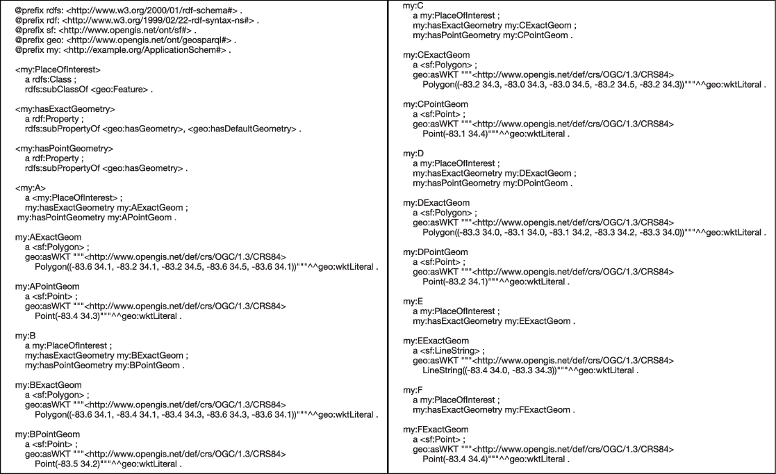
Figure 2 shows the GeoSPARQL RDF representation (RDF Turtle syntax) of an application-specific spatial data in Figure 1.

Figure 1.

The application-specific spatial data

Figure 2.

The GeoSPARQL RDF representation of the spatial data in Figure 1

(2) W3C Basic Geo Vocabulary (W3C GEO, 2003)

W3C Basic Geo Vocabulary (W3C GEO 2003) provides a basic RDF vocabulary for representing points, using WGS84 (World Geodetic System, 1984) as a reference datum.

The vocabulary defines a class ‘Point’, whose members are points. Points can be described using ‘lat (latitude)’, ‘long (longitude)’, and ‘alt (altitude)’ properties, as well as with other RDF properties defined elsewhere. The ‘lat’ and ‘long’ properties take literal (i.e. textual values), each in decimal degrees. The ‘alt’ property is decimal meters about local reference ellipsoid.

The following is a simple example.

Although the W3C Basic Geo vocabularies is widely used to describe WGS84 coordinates, it is does not allow the description of geometric shapes, such as the border of a country (Salas & Harth, Reference Salas and Harth2011). Similarly, as mentioned in Battle and Lolos (2012) and OGC GeoSPARQL (2012), The simple W3C Basic Geo vocabularies have limitations, for example, the inability to specify different datums and coordinate systems, and were therefore not used in GeoSPARQL. The most existing geometry data encoded using these simple W3C Basic Geo vocabularies can easily be converted into GeoSPARQL representations.

Moreover, GeoRSS (www.georss.org) provided support for more geometric objects (such as lines, rectangles, or polygons) and GML application profiles. It is designed as a lightweight, community-driven way to extend existing RSS (really simple syndication) feeds with simple geographic information. The main purpose of GeoRSS standard is not to represent geometry data in RDF, but to provide for encoding location in an interoperable manner so that applications can request, aggregate, share and map geographically tag feeds. The encoding may be expressed in a concrete form such as XML, RDF. GeoJSON (https://geojson.org) is a geospatial data interchange format based on JavaScript Object Notation (JSON) and can encode a variety of shapes (points, polygons, etc.).

Note that a further report is discussed by the W3C Geospatial Incubator Group (GeoXG) (W3C Geospatial Vocabulary 2007) to discuss the need for updating the W3C Basic Geo Vocabulary (W3C GEO 2003) following the GeoRSS feature model, and to allow for the description of points, lines, rectangles, and polygon geometries and their associated features.

(3) NeoGeo (Salas & Harth, Reference Salas and Harth2011 ; Salas et al ., Reference Salas and Harth2011 )

By analyzing the representation of several existing geospatial datasets, Salas et al. (Reference Salas and Harth2011) distill an integration vocabulary NeoGeo, which covers the core set of classes and properties in existing data. They identify four main kinds of representation (point, bounding box, points in lists, points using a single property and literals) to support typical geometric objects (Geometry, Point, MultiPoint, LineString, MultiLineString, LinearRing, Polygon, MultiPolygon, GeometryCollection), as well as WKT serialization.

In the NeoGeo Vocabulary, everything is represented as an RDF resource, maximizing the vocabulary’s expresivity. For example, the list of nodes, which form a polygon is an RDF collection containing an RDF resource for each node. That is, the polygons and lines are represented by an RDF collection of W3C Basic Geo points (W3C GEO 2003). The basic classes are spatial:Feature and geom:Geometry, which is connected via the geom:geometry property. In more detail, a geometry vocabulary (http://geovocab.org/geometry) for describing geographical regions in RDF is defined, which includes several classes (e.g. LineString and Polygon) and several properties (e.g. boundary and exterior). Also, a spatial vocabulary (http://geovocab.org/spatial) for describing RCC-8 topological relations between features is defined, which include a class Feature and several properties (e.g. DC(x, y) for ‘x is disconnected from y’ and EC(x, y) for ‘x is externally connected with y’).

The following example shows that Karlsruhe is a spatial:Feature, and is related to http://example.org/geo/kageo, which is a geom:Geometry. And the Argentina is defined to be a tangential proper part (RCC-8 TTP) of South America, and is externally connected (RCC-8 EC) to other countries like Uruguay, Brazil, Paraguay, Bolivia, and Chile.

Moreover, they publish two geospatial datasets NUTS and GADM, and also develop an algorithm for finding equivalences for geometric shapes across multiple datasets for integration and mapping of multiple datasets.

(4) Spatial Literals in RDF (Brodt et al. , Reference Brodt, Nicklas and Mitschang2010)

Brodt et al. (Reference Brodt, Nicklas and Mitschang2010) represent spatial features in RDF as literals of a complex geometry type and store them in RDF literals. The literals contain the spatial features expressed in the Well-Known Text (WKT) format, as standardized in the OpenGIS Simple Features Specification (OGCSF). The literals carry a type URI, which denotes that the literal is to be processed as a spatial feature rather than as an ordinary string. For example, the position of a gas station can be represented as <:Station1234 :locatedAt ‘POINT (48.77 9.18)’ ^ ^ geordf:geography>, where geordf is the namespace prefix of http://example.org/geo.

Note that the approach does not assign a IRI to a spatial feature, so that it cannot be directly referenced or augmented by metadata. Still, the place resources would keep all information related to geographic coordinates in the single RDF statement, which carries the spatial literal. All further statements related to the place resource are ‘ordinary RDF and can be designed in any ontology. The following example shows the gas station using a place resource:

(5) GeoRDF (GeoRDF)

GeoRDF was intended as an RDF compatible profile for geographic information (points, lines, and polygons). The representation of the points is similar to the W3C Basic Geo Vocabulary (W3C GEO 2003). The lines and polygons can be represented by ‘simple’ profile or ‘complex’ profile. The ‘simple’ profile is based on Mikel’s extension of the geo schema (http://mapufacture.com) and uses lists of comma-separated lat, long pair values to describe both lines and polygons as shown in the following example.The ‘complex’ profile is based on Chris Goad’s more complex formulation (http://fabl.net/lib/geometry/1.1/revision1.html) and uses an rdf:Seq to express a list of points that are a line, a polyline, or a polygon. Its two vocabularies (RDFGeom and its 2d companion RDFGeom2d) provide a framework that is extensible via subclassing to all kinds of geometric data.

(6) RDF ⁱ (Nikolaou & Koubarakis, Reference Nikolaou and Koubarakis2012 , Reference Nikolaou and Koubarakis 2013 )

Nikolaou and Koubarakis (Reference Nikolaou and Koubarakis2012); (Reference Nikolaou and Koubarakis2013) address the problem of representing and querying incomplete geospatial information in RDF using the framework named RDF ⁱ (where ‘i’ stands for ‘incomplete’), which extends RDF with the ability to represent property values that exist, but are unknown or partially known, using a quantifier-free formula of a first-order constraint language $\mathcal{L}$ . Formally, RDF ⁱ extends the concept of an RDF graph to the concept of an RDF ⁱ database, which is a pair (G, $\phi$ ) where G is an RDF graph possibly containing triples with e-literals in their object positions, and $\phi$ is a quantifier-free formula of $\mathcal{L}$ . RDF ⁱ extends RDF with the ability to define a new kind of literals for each datatype. These literals are called e-literals (‘e’ comes from the word ‘existential’). It should be noted that e-literals are allowed to appear only in the object position of triples in RDF ⁱ .

For example, a real-world situation that corresponds to a hotspot would be to state that there is a geographic region with unknown exact coordinates where a fire is taking place, and that region is included in a known 3 km by 3 km rectangle. Such case can be represented by RDF ⁱ as shown in the following example:

The fire fire1 (red area of Figure 3) is asserted to have taken place inside region $\_$ R1, which is an e-literal datatype and is asserted to be inside the rectangle formed by the points (6,8) and (23,19) (rectangle P of Figure 3). This is stated with a constraint expressed in the language PCL (Polygon Constraint Language), a first-order constraint language that allows to represent topological properties for polygons. NTPP is the ‘non-tangential-proper-part’ relation of RCC-8 (Randell et al., Reference Randell, Cui and Cohn1992). In general, constraints in PCL can be used to express qualitative and quantitative spatial information about regions in $\mathbb{Q}^{2}$ .

Figure 3.

Rectangles mentioned in the example of RDF ⁱ

3.2 Spatial RDF storage, querying, and performance assessment

Facilities for the storage and querying of large quantities of spatial data are important to many applications, and thus many geographic information systems and spatial databases are developed (Paton et al., Reference Paton, Williams and Dietrich2000). After RDF is employed to represent massive spatial application data as introduced in Section 3.1, there has been significant community and research interest in storing and querying geospatial data based on RDF management techniques. Accordingly, some spatial RDF storage and querying techniques are proposed.

For storing and querying spatial RDF data, some native architectures and hybrid architectures are developed. As mentioned in Quoca et al. (Reference Quoca, Serranob and Mauc2019), the native architecture needs to implement the data indexing system, the query engine, and the physical storage. The hybrid architecture uses existing systems as sub-components for the processing needed. Note that the data indexing has vital roles in the performance of data insertion and query. The query engine may include a query parser (parsing the input query), a query optimizer (determining the most efficient way to execute a given query by considering all the possible query execution plans), and query executor (processing and returning the query results). The physical storage can be classified into two types, namely native (persistent disk-based and main memory-based) and non-native storage (relies on the relational database management system RDBMS to store RDF data permanently). Moreover, as also mentioned in Kolas (Reference Kolas2008) and Patroumpas et al. (Reference Patroumpas, Alexakis and Giannopoulos2014), there are some primary types of spatial queries that should be covered, for example, location queries, range queries, spatial joins, and nearest neighbor search.

In addition, the performance study and assessment of spatial RDF querying and storage techniques is crucial to select a suitable RDF engine for some applications and promote the development of RDF data management techniques. In the following, the Subsection 3.2.1 will first summarize and compare the existing spatial RDF storage and querying techniques. Then, the Subsection 3.2.2 will summarize the existing work about the performance assessment of spatial RDF querying and storage techniques.

3.2.1 Spatial RDF storage and querying

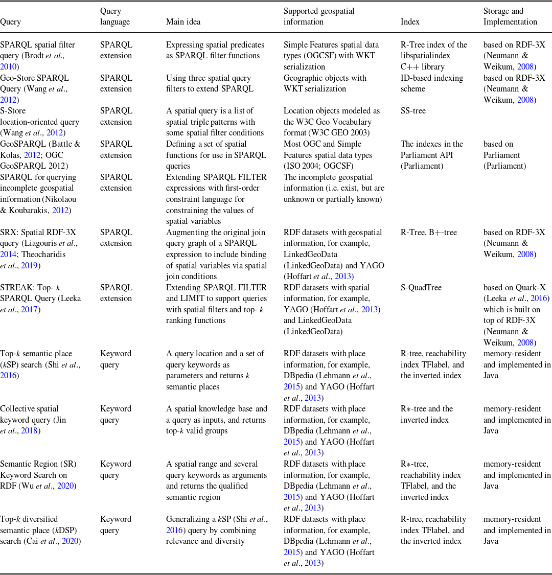
Table 2 first summarizes and compares the spatial RDF storage and querying techniques according to their support for spatial data management.

Table 2.

Qualitative comparison of spatial RDF storage and querying techniques

(1) SPARQL spatial filter queries (Brodt et al. , Reference Brodt, Nicklas and Mitschang2010)

In order that the data management systems are capable of querying large amounts of RDF data and supporting spatial query predicates, Brodt et al. (Reference Brodt, Nicklas and Mitschang2010) model spatial features as typed complex literals, and define spatial predicates as filter functions in SPARQL. The literals contain the spatial features expressed in the Well-Known Text (WKT) format, as standardized in the OpenGIS Simple Features Specification (OGCSF) as mentioned in Section 3.1. On this basis, they express spatial predicates as SPARQL filter functions on this type. This makes it possible to use W3C standardized SPARQL query language as-is, that is, without any modifications or extensions for spatial queries.

In more detail, the approach to express spatial query predicates in SPARQL uses filter functions that are identified by an IRI. It uses the functions of the OpenGIS Simple Features Specification (OGCSF) and defines an IRI for each of them. The filter functions act on variables, which bind a spatially typed literal as mentioned in Section 3.1. Geometry constants to compare the value of the variable are specified as spatially typed literals too; they are given in the well-known text (WKT) format and carry an IRI denoting the spatial type. They also implement a spatial index based on the R-Tree index of the libspatialindex C++ library (http://sourceforge.net/projects/spatialindexlib). The following example shows a fully standard-compliant SPARQL query to find all gas stations within a given area that specifies the spatial query predicate as a filter function (where geordf and geo are the namespace prefixes of http://example.org/geo and http://www.w3.org/2003/01/geo/wgs84_pos, respectively).

They finally implement the approach based on the architecture of the triple store RDF-3X (Neumann & Weikum, Reference Neumann and Weikum2008) and make some modifications to RDF-3X with spatial functionality. The evaluation shows that some of the modifications do create some extra overhead for queries selecting very large amounts of spatial features, but excellent performance for most common spatial query types.

(2) Geo-Store: spatially augmented SPARQL query (Wang et al ., Reference Wang, Ku and Chen2012)

Wang et al. (Reference Wang, Ku and Chen2012) propose Geo-Store, a novel spatially augmented SPARQL evaluation system. By using spatial query filters to extend the standard SPARQL query language, Geo-Store can handle complex spatial queries with common spatial constraints. These spatial filters are designed based on spatially aware mapping (SAM) scheme. With SAM, spatial data can be preprocessed and encoded with their Hilbert values by using the Hilbert curve to accelerate spatial query evaluation without any compromise in accuracy.

The major components of Geo-Store include a spatially aware mapping (SAM) module, an internal processing (IP) module, a spatial query analyzer (SQA) module, and a dictionary decoding (DD) module. By the SAM module, Hilbert curves are generated and Hilbert values (integers) of the literals containing coordinate information (latitude/longitude) are calculated and then appended to the original triple data source as location indicators. The IP module maintains in memory of all six possible permutations of <s p o> in six separate indices (i.e. SPO, SOP, OSP, OPS, PSO, and POS indices), and all six indices consist of integer IDs, which are assigned by SAM. Further, spatial queries are expressed by using spatial query filters in the SQA module. If a spatial filter is detected by SQA, the SQA will employ SAM to identify a list of Hilbert values (serving as location indicators) that are involved with the filter. Then, the SQA will translate the derived Hilbert values into query patterns and append them as clauses to the original SPARQL query expression. For multiple spatial query filters, the SQA will apply intersection operations to find the geographic locations satisfying all the spatial filters. Finally, the DD module transforms the obtained IDs back to their original literals as the query results.

Geo-Store supports three spatial filters, namely window filter, range filter, and nearby filter. These filters operate on geographic objects (and variable bindings) expressed in the Well-Known Text (WKT) format.

1. • Window filter: specifies a rectangular geographic constraint on a SPARQL variable. The syntax of this filter is within(?var, xmin, ymin, xmax, ymax). The following gives an example of a SPARQL query with a window filter. The query defines three query variables (?e, ?name, and ?location) and returns the name and location of records whose locations satisfy the window filter.

1. • Range filter: specifies a constraint region that is within a certain distance of a geographic point. This filter essentially defines a circular region around a central point. There are two variations of this filter, the first takes literal coordinates of the center and the second takes a variable as the center.

2. • Nearby filter: sorts the bounded values based on the Euclidean distance between the bounded values and a center point, and returns the closest k bindings.

The Geo-Store system is built on top of RDF-3X (Neumann & Weikum, Reference Neumann and Weikum2008), a scalable RDF triple store. Moreover, it provides a graphical query interface for the users to easily compose spatial and non-spatial constraints to construct SPARQL queries.

(3) S-store: location-oriented spatial SPARQL query (Wang et al ., Reference Wang, Ku and Chen2012)

In order to realize the location-oriented spatial information query, Wang et al. (Reference Wang, Ku and Chen2012) propose spatial SPARQL (a variant of SPARQL language) for querying RDF data with spatial features. In their work, a spatial triple pattern is a four-tuple s, p, o, l, where s, p, o, and l represent subject, predicate, object and location, respectively, and the ‘location’ feature is modeled as the W3C Geo Vocabulary format (W3C GEO 2003). In this case, a spatial query is a list of spatial triple patterns with some spatial filter conditions. If there’s no spatial filter condition, the spatial query is reduced to a traditional SPARQL query. For example, a location-oriented spatial query about a person who died in a popular place near coordinates (48.39841,9.99155) can be expressed as follows:

where sl(?y) denotes the spatial label of variable ?y. Besides, dist(a, b) < r denotes the Euclidean distance between a and b should below the threshold r, where a and b should be a specific location or a variable. If either of a and b is a constant, the query is called a range query. If both of a and b are variables, the query is called a spatial join query. Note that a spatial query can be a range query and a spatial join query at the same time.

Further, they classify the entities into two categories: the spatial entities and the non-spatial entities. Based on these two categories, they define a tree-style index structure (called SS-tree), which is a hybrid tree-style index integrating the semantic features and the spatial features. They finally evaluate their approach on YAGO2 (Hoffart et al., Reference Hoffart, Suchanek and Berberich2013).

(4) GeoSPARQL (Battle & Kolas, Reference Battle and Kolas2012 ; OGC GeoSPARQL, 2012)

In order to solve the problem of spatial inference with the amount of spatial context data, a SPARQL extension language, called GeoSPARQL, was developed in OGC GeoSPARQL (2012) and Battle and Kolas (Reference Battle and Kolas2012) for unifying the data access of the geospatial Semantic Web. GeoSPARQL is also the OGC (Open Geospatial Consortium) standard. GeoSPARQL defines a vocabulary for representing geospatial data in RDF as mentioned in Section 3.1, and it defines an extension to the SPARQL query language for processing geospatial data. Here, we will introduce the query part of GeoSPARQL in detail.

The GeoSPARQL specification contains three main components:

1. 1. The definition of a vocabulary to represent features, geometries, and their relationships as mentioned in Section 3.1.

2. 2. A set of domain-specific, spatial functions for use in SPARQL queries.

3. 3. A set of query transformation/rewrite rules, which allows for an additional layer of abstraction in SPARQL queries.

Regarding the spatial functions for use in SPARQL queries, GeoSPARQL provides two different types of functionality. First, there are operator functions, which take multiple geometries as predicates and produce either a new geometry or another datatype as a result. An example of this is the function geof:intersection (where geof is the prefix of http://www.opengis.net/def/function/geosparql/). This function takes two geometries and returns a geometry that is their spatial intersection. Other functions like geof:distance produce an xsd:double as a result. The second type of functionality is Boolean topological tests of geometries. An example of the topological functions is geof:sfContains, which returns true if one geometry contains another geometry (where sfContains represents the relartion contains of Simple Features relations (ISO 2004; OGCSF).

For example, given the spatial RDF data in Figures 1 and 2 in Section 3.1, the query ‘Find all features that feature my:A contains, where spatial calculations are based on my:hasExactGeometry.’ can be expressed in the following GeoSPARQL query:

In this example, the property geo:asWKT is defined to link a geometry with its WKT serialization as introduced in Section 3.1, and the sameTerm returns TRUE if term1 and term2 are the same RDF term. After running the query above, the features my:B and my:F in Figure 1 will be returned.

Moreover, they also have worked to update the open-source triple store Parliament to support GeoSPARQL. In addition, some work is attempted to further extend or use the GeoSPARQL for special applications. The work in Zhao et al. (Reference Zhao, Zhang and Anselin2015) proposes a parallel approach for improving the query performance of geospatial ontology in a GeoSPARQL query by separating spatial and non-spatial components. The work in Zhang et al. (Reference Zhang, Beetz and de Vries2018) proposes a BimSPARQL query language by extending SPARQL functions for querying Industry Foundation Classes (IFC) building 3D geometry data. Several simpler approaches in Xiao et al. (Reference Xiao, Huang and Zhai2009); Zhai et al. (Reference Zhai, Huang and Xiao2010) also discuss the need for adding topological predicates to SPARQL, and the OGC Simple Features relations (ISO 2004; OGCSF) and a subset of geometries are used as the basis for their ontologies.

(5) SPARQL for querying incomplete geospatial information (Nikolaou & Koubarakis, Reference Nikolaou and Koubarakis2012 )

As mentioned in Section 3.1, an RDF extension model, called RDF ⁱ is proposed for representing the incomplete geospatial information (i.e. exist, but are unknown or partially known) (Nikolaou & Koubarakis, Reference Nikolaou and Koubarakis2012; Nikolaou & Koubarakis, Reference Nikolaou and Koubarakis2013). Further, for querying the incomplete geospatial information, Nikolaou and Koubarakis (Reference Nikolaou and Koubarakis2012) define an extension language of SPARQL. For example, the query ‘Find all fires that have occurred in a region which is a non-tangential proper part (NTPP of RCC-8 (Randell et al., Reference Randell, Cui and Cohn1992)) of rectangle Q $_{1}$ of Figure 3’ may be expressed by the extension of SPARQL as follows:

From the example, they extend FILTER expressions of standard SPARQL and allow the expression of a first-order constraint language for constraining the values of spatial variables. More detailed definitions for the extension of SPARQL language can be found in Nikolaou and Koubarakis (Reference Nikolaou and Koubarakis2012).

(6) SRX: Spatial RDF-3X query (Liagouris et al ., Reference Liagouris, Mamoulis and Bouros2014 ; Theocharidis et al ., Reference Theocharidis, Liagouris and Mamoulis2019)

For efficiently supporting spatial queries, such as range selections (e.g. find entities within a given range) and spatial joins (e.g. find pairs of entities whose locations are close to each other), Liagouris et al. (Reference Liagouris, Mamoulis and Bouros2014) propose an extension for RDF stores that supports efficient spatial data management, including providing effective coding schemes for entities with spatial locations, introducing dynamic spatial filters and spatial join algorithms, and giving some optimizations that minimize the overhead of geometry and dictionary accesses.

In more detail, they present the details of a system by extending the open-source RDF-3X engine (Neumann & Weikum, Reference Neumann and Weikum2008) in the following several aspects (where RDF-3X encodes all values that appear in <s p o> triples by identifiers with a help of a dictionary and models the RDF knowledge base as a single, long table of ID triples. A SPARQL query can then be modeled as a multi-way join on the triples table.):

1. • Index Support for Spatial Queries. The system includes a spatial index R-tree for the geometries associated to the spatial entities.

2. • Spatial Encoding of Entities. The system encodes spatial approximations inside the IDs of entities (i.e. resources) associated to spatial locations and geometries.

3. • Spatial Join Algorithms. The system designs spatial join algorithms tailored to the above encoding scheme.

4. • Spatial Query Optimization. The system augments the original join query graph of a SPARQL expression to include the binding of spatial variables via spatial join conditions. That is, the Filter clause in a SPARQL query may include one or more spatial predicates. The system considers only WITHIN range predicates (for spatial selections, see Figure 4) and DISTANCE predicates (for spatial joins, see Figure 4). For example, an RDF knowldege base with spatial information and a corresponding SPARQL query including a spatial join predicate is shown in Figure 4.

   Figure 4.

   RDF spatial data and SPARQL spatial join predicate query in SRX

   

They experimentally evaluate the system using two real datasets LinkedGeoData (LDG) and YAGO2 (Hoffart et al., Reference Hoffart, Suchanek and Berberich2013). The work is further extended in Theocharidis et al. (Reference Theocharidis, Liagouris and Mamoulis2019), where a system called SRX (Spatial RDF-3X) was implemented, which extends RDF-3X with support for three types of spatial queries: range selections and spatial joins as mentioned above, and spatial k -nearest neighbors (e.g. find the three closest entities from a given location).

(7) STREAK:Top- k SPARQL Queries (Leeka et al ., Reference Leeka, Bedathur and Bera2017)

Leeka et al. (Reference Leeka, Bedathur and Bera2017) present an RDF data management system called STREAK to process kinds of queries with spatial filters (including complex joins, higher order relationships over spatially enriched datasets), along with top- k requirements over arbitrary user-defined ranking functions, expressed in the order by the LIMIT clauses. They consider the following SPARQL query structure:

where the FILTER clause restricts solutions to those that satisfy the spatial predicates. In their work, they focus only on the use of DISTANCE predicate for distance joins. The ORDER BY clause helps to establish the order of results using a user-defined ranking function. The LIMIT clause controls the number of results returned. Together, ORDER BY and LIMIT form the top- k result retrieval with ad hoc user-defined ranking function.

In the STREAK system, they present a S-QuadTree index, a novel RDF-specific extension of Quadtree (Finkel & Bentley, Reference Finkel and Bentley1974) (a popular in-memory spatial index structure). S-QuadTree stores all the spatial entities in the knowledge graph, and embeds the associated soft-schema information. Further, they propose a spatial join algorithm and an adaptive query plan generation algorithm called Adaptive Processing for Spatial filters (APS), which switches with very low plan-switching overhead to select between alternate query plans, based on a novel spatial join cost model.

They implement these features within their previous framework Quark-X (Leeka et al., Reference Leeka, Bedathur and Bera2016), a top-k SPARQL processing system based on RDF-3X (Neumann & Weikum, Reference Neumann and Weikum2008). They evaluate their approach on LinkedGeoData (LGD) and YAGO2 (Hoffart et al., Reference Hoffart, Suchanek and Berberich2013).

(8) Spatial Keyword Search on RDF data (Shi et al ., Reference Shi, Wu and Mamoulis2016 ; Jin et al ., Reference Jin, Shin and Jo2018 ; Cai et al ., Reference Cai, Kalamatianos and Fakas2020 ; Wu et al ., Reference Wu, Hou and Xiao2020)

Consider that RDF data are traditionally accessed using SPARQL as mentioned in Section 3.1. Some work stated that SPARQL may be not friendly to common users, since query issuers need to understand the language itself and to be aware of the data domain, and thus it limits data access mostly to domain experts. This leaves room for a keyword search model on RDF data. Therefore, some work investigated the spatial keyword search on RDF data.

Top- k relevant semantic place (kSP) search. Shi et al. (Reference Shi, Wu and Mamoulis2016) propose a novel way of searching spatial RDF data, namely top- k relevant Semantic Place retrieval (k SP) query. It takes a query location and a set of query keywords as parameters and combines keyword-based and location-based retrieval. The query returns k semantic places that are subgraphs rooted at place entities that have associated locations.

Semantic Region (SR) search. Wu et al. (Reference Wu, Hou and Xiao2020) propose a generalization of semantic place retrieval, namely semantic region (SR) retrieval. Specifically, an SR query takes a spatial range and a set of query keywords as arguments and returns the qualified semantic region that minimizes a scoring function. The semantic region is composed of a subgraph T(r, P) connecting a set of places that are in the query spatial range and the so-called keyword-relevant paths of the query keywords. The scoring function considers both the graph proximity of the occurrences of query keywords in the RDF graph to the places and the graph proximity among the places. An SR query aims to retrieve multiple places that are spatially close to the query location such that each place is relevant to one or more the query keywords. An algorithm and optimization techniques are proposed for the efficient processing of SR queries. The proposed techniques are evaluated on DBpedia (Lehmann et al., Reference Lehmann, Isele and Jakob2015) and YAGO (Hoffart et al., Reference Hoffart, Suchanek and Berberich2013), two large real RDF datasets. The results show that applying all techniques enables processing SR queries efficiently.

Top-k diversified semantic place (kDSP) search. Cai et al. (Reference Cai, Kalamatianos and Fakas2020) introduce diversified spatial keyword search on RDF data. Their framework enables a trade-off between relevance and diversity. Namely, the output places, in addition to being relevant to the query, should minimize the number of common nodes in their subgraphs and should have diverse locations w.r.t. direction. To this end, they propose a top- k diversified semantic place (k DSP) query, which generalizes the above k SP (Shi et al., Reference Shi, Wu and Mamoulis2016) query by combining a relevance function to the query and a diversity function on the set of query results that considers their relative location and content. Note that all of the keyword search approaches mentioned above use the index techniques such as R-tree, reachability index TFlabel, and the inverted index.

Collective spatial keyword query. Jin et al. (Reference Jin, Shin and Jo2018) stated that (k SP) query (Shi et al., Reference Shi, Wu and Mamoulis2016) aims to find a subtree that is rooted at a place vertex, covers all query keywords, and minimizes a ranking function. But user requirements may not be satisfied by a single subtree in some application scenarios. A group of subtrees should be combined together to collectively cover the query keywords. To this end, they propose and study a novel way of searching a spatial knowledge, namely collective spatial keyword query on a knowledge base (CoSKQ-KB). It takes a spatial knowledge base and a query as inputs, and returns top- k valid groups w.r.t. a ranking function. A valid group is composed of several semantic places, that is, the subtrees rooted at place vertices, and the member semantic places collectively cover all the query keywords. A ranking function is designed to measure the spatial closeness as well as the semantic keyword relevance of a valid group w.r.t. a query. The valid group with a lower ranking score has a higher chance to satisfy a user’s requirement. Further, they propose two algorithms for CoSKQ-KB, BCK and iSCK. BCK employs efficient pruning techniques to reduce search spaces. iSCK improves BCK with carefully designed dynamic bounds to terminate iterations earlier. Also, the R*-tree and the inverted indexes are used and the empirical experiments on DBpedia (Lehmann et al., Reference Lehmann, Isele and Jakob2015) and YAGO (Hoffart et al., Reference Hoffart, Suchanek and Berberich2013) are conducted to show the efficiency and effectiveness of the proposed algorithms.

(9) Some early spatial RDF storage and querying techniques

As already mentioned in Athanasiou et al. (Reference Athanasiou, Bezati, Giannopoulos, Patoumpas and Skoutas2012), Battle and Kolas (Reference Battle and Kolas2012), and Patroumpas et al. (Reference Patroumpas, Alexakis and Giannopoulos2014), there are several early spatial RDF storage techniques, including:

1. • Parliament: a high-performance triple store and reasoner, which is designed for the Semantic Web. The storage structure consists of a resource table, a statement table, and a resource dictionary. It also includes a rule engine for the inference, and currently supports RDFS plus parts of OWL. Parliament is compatible with the RDF, RDFS, OWL, SPARQL. With respect to the geospatial RDF, it supports GeoSPARQL standards, allowing GeoSPARQL data to be indexed and provides a query engine that supports GeoSPARQL queries using standard R-trees index.

2. • Virtuoso Universal Server: a middleware and database engine hybrid. For storing RDF data, it implememts a quad GSPO (i.e. Graph, Subject, Predicate, Object), and all quads are stored in one table that relies on an underlying RDBMS (relational database management system). SPARQL is embedded and translated into SQL for querying RDF data stored in the database. With respect to the geospatial RDF, it supports the W3C Basic Geo Vocabulary points (W3C GEO 2003) as mentioned in Section 3.1. Topological relations can be queried, but are limited to some built-in predicates (st $\_$ intersects, st $\_$ contains, st $\_$ within). Note that spatial types and functions are limited in Virtuoso and currently not compliant with GeoSPARQL.

3. • GraphDB (former OWLIM): a family of semantic repositories rebranded as GraphDB that intend to offer scalability, loading, and query evaluation performance for native RDF engines. It is compatible with all the common RDF syntaxes (XML, N3, N-Triples, Turtle, TRIG, TRIX) and supports the SPARQL, and also includes an inference engine. With respect to the geospatial RDF, it supports 2-dimensional points that use the W3C Basic Geo Vocabulary (W3C GEO 2003) with coordinates in WGS84, and supports the SPARQL to query points within ad hoc rectangles, polygons and circles and to compute distances (in kilometers) between points.

4. • uSeekM: an add-on library for Semantic Databases (also known as Triple-stores, Quad-stores, or RDF-databases) that use the Sesame (an open-source framework for storing, querying, and analyzing RDF data, now is RDF4J project (Sesame)) Java interface. uSeekM adds powerful indexing and querying capabilities to Semantic Databases, and provides integrations with other tools and frameworks. Most of its functionality is provided through wrappers. With respect to the geospatial RDF, it supports all OGC geometry types specified in the OGC Simple Features Implementation Specification for SQL and most operations in the GeoSPARQL standard.

5. • Stardog: a commercial knowledge graph product that supports parsing, storing, inferencing, and querying RDF data. It supports SPARQL 1.1 and both ontological and rule-based reasoning with a query rewriting strategy. It supports a few GeoSPARQL query functions.

3.2.2 Performance assessment of spatial RDF storage and querying techniques

With the widely use of RDF for representing and processing spatial data, some spatial RDF querying and storage framework are proposed as mentioned above. Accordingly, some work are developed for assessing spatially enabled RDF querying and storage techniques. Before the GeoSPARQL, in the early work, Kolas (Reference Kolas2008) extends LUBM (Lehigh University Benchmark, a well-known RDF benchmark) to include spatial entities and test the performance of spatially enabled RDF stores. Afterward, the GeoKnow project (2012) (Athanasiou et al., Reference Athanasiou, Bezati, Giannopoulos, Patoumpas and Skoutas2012) provides a survey and evaluation of spatially enabled RDF stores, and the selective stores in GeoKnow include Virtuoso, Parliament, OWLIM, uSeekM, and Strabon (a storage and query module for spatiotemporal RDF data as will be mentioned in the next Section 4), as well as spatially enabled relational databases, that is, Oracle Spatial and PostgreSQL with PostGIS extension. Battle and Kolas (Reference Battle and Kolas2012) demonstrate the geospatial capacity of Parliament and successfully achieved lots of GeoSPARQL-compliant queries as mentioned in Section 3.2.1. Patroumpas et al. (Reference Patroumpas, Alexakis and Giannopoulos2014) perform an evaluation of the performance of the geospatial RDF stores.

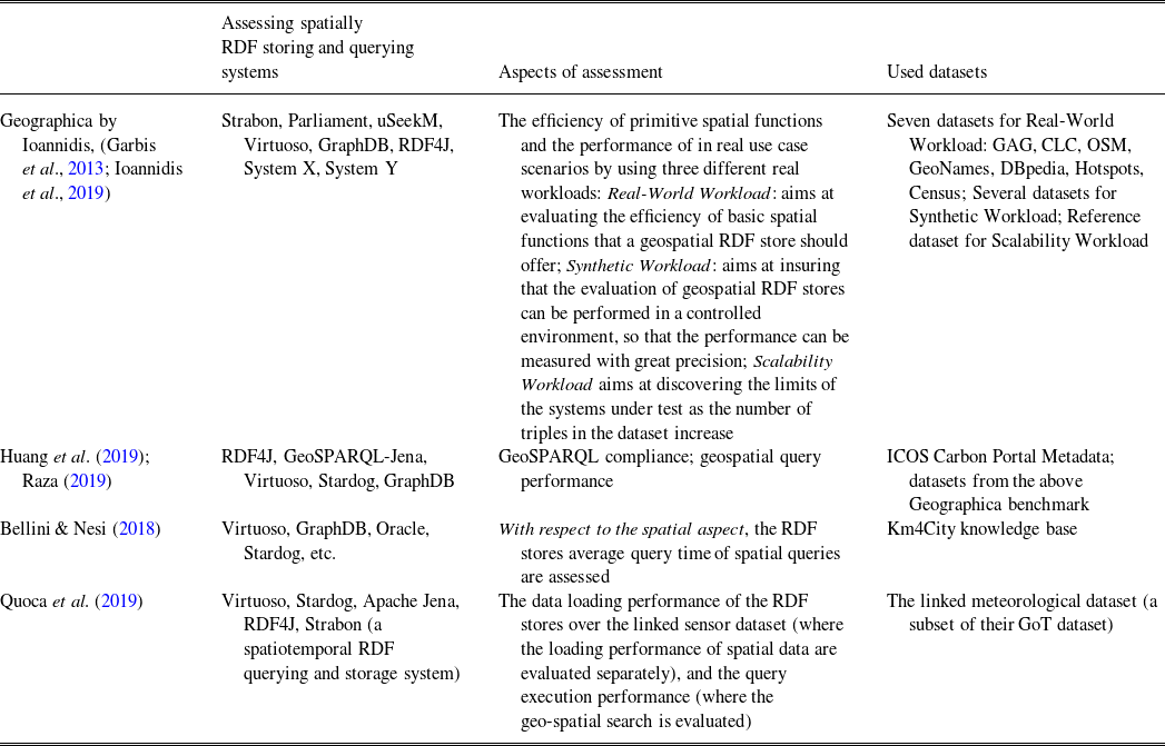
Table 3 further summarizes and compares several recent work about the performance study and assessment of spatial RDF querying and storage techniques.

Table 3.

Performance assessment of spatial RDF storage and querying techniques

As shown in Table 3, (Huang et al., Reference Huang, Raza and Mirzov2019; Raza, Reference Raza2019) comprehensively assess and benchmark five popular and well-known spatially enabled RDF stores, that is, RDF4J, GeoSPARQL-Jena, Virtuoso, Stardog, and GraphDB. Along with the investigation of features, the performance evaluation of these RDF stores has also been conducted by measuring the execution times of a set of GeoSPARQL queries. The evaluation query set consists of non-topological, spatial selection as well as spatial join queries adopted from a spatial benchmark, Geographica. It is encouraging to see the increasing maturity of the technical environment for the support of geospatial linked data, as well as the increasing compliance with GeoSPARQL compared with previous benchmarks.

Ioannidis et al. (Reference Ioannidis, Garbis and Kyzirakos2019) revisit their previous Geographica benchmark in 2013 (Garbis et al., Reference Garbis, Kyzirakos and Koubarakis2013), which uses both real-world and synthetic data to test the performance and functionality of geospatial RDF stores. In the new version Geographica 2, eight systems (Strabon, Parliament, uSeekM, Virtuoso, GraphDB, RDF4J, System X, System Y) are evaluated out of which six adequately support GeoSPARQL and two offer limited spatial support. Geographica 2 tests the efficiency of primitive spatial functions in RDF stores and the performance of the RDF stores in real use case scenarios by using the following three different real workloads:

1. • Real-World Workload: aims at evaluating the efficiency of basic spatial functions that a geospatial RDF store should offer. In addition, this workload includes five real use case application scenarios (three typical application scenarios, namely ‘Geocoding’, ‘Reverse Geocoding’, ‘Map Search and Browsing’; two more sophisticated scenarios, namely ‘Rapid Mapping for Fire Monitoring’, ‘Computing Statistics of Geospatial Datasets’).

2. • Synthetic Workload: aims at insuring that the evaluation of geospatial RDF stores can be performed in a controlled environment, so that the performance can be measured with great precision. It relies on a generator that produces synthetic datasets of various sizes and instantiates query templates that can produce queries with varying thematic and spatial selectivity. The synthetic workload generator produces SPARQL queries corresponding to spatial selection and spatial joins using the two query templates.

3. • Scalability Workload: aims at discovering the limits of systems under test as the number of triples in the dataset increase. Each system is tested against six increasingly bigger, proper subsets of the reference dataset. For each system-dataset combination, they measure (i) the repository size on disk, (ii) the bulk loading time taking into consideration the limitations of loading methods of each system, and (iii) the response time in three queries which represent a spatial selection, a heavy spatial join with high spatial selectivity and a lighter spatial join with lower spatial selectivity.

Bellini and Nesi (Reference Bellini and Nesi2018) assess several well-known RDF stores, including Virtuoso, GraphDB, Oracle, and Stardog, for semantically enabled smart city services. The assessment model allows a full understanding of whether an RDF store is suitable to be used as a basis for Smart City modeling and applications. The benchmark is based on the Florence Smart City model, and the used datasets and tools are available online. With respect to the spatial aspect, the Spatial search at Basic level (meaning that it is able to index and retrieve only geolocated points) or at Advanced level (meaning that it is able to index complex shapes, e.g. polylines) are considered, and the RDF stores average query time of spatial queries are assessed.

Quoca et al. (Reference Quoca, Serranob and Mauc2019) present the empirical studies for selecting a suitable RDF engine for Linked Sensor Data. The selected RDF stores include Virtuoso, Stardog, Apache Jena, RDF4J, Strabon. And the evaluation coveres two aspects: the data loading performance of the RDF stores over the linked sensor dataset (where the loading performance of spatial data are evaluated separately) and the query execution performance (where the geo-spatial search is evaluated). Here, besides the overall query execution time, they also measure the execution performance of query parsing, query optimization and query execution. The query parsing time is calculated from the time the system retrieves the query string to the time the query algebra tree is generated. Similarly, the query optimization process is considered starting from the time the query tree and it is finished when an execution plan is delivered. For simplicity, any other runtime decisions are considered as part of the query execution rather than part of the query optimization. The query execution is finished when the last result has been received. The evaluation is conducted over the linked meteorological dataset, a subset of their GoT dataset (a unified integrated and live view for heterogeneous Internet of Things data sources using Linked Data, called the Graph of Things-GoT, see http://graphofthings.org/).

3.3 Spatial RDF datasets and management tools

With the application of RDF in spatial data process, some spatial RDF datasets and management tools are developed. Several common spatial RDF datasets include:

1. • LinkedGeoData (LGD, Stadler et al., Reference Stadler and Lehmann2012): a core for a Web of Spatial Open Data. It is an effort to add a spatial dimension to the Web of Data/Semantic Web. LinkedGeoData uses the information collected by the OpenStreetMap project and makes it available as an RDF knowledge base according to the Linked Data principles. It interlinks this data with other knowledge bases in the Linking Open Data initiative.

2. • GeoNames: a geographical database that covers all countries and provides Linked Data under a Creative Commons attribution license. It provides information for over eight million geospatial features. The data are exposed via an RDF webservice that exposes information on a per resource basis.

3. • DBPedia (Lehmann et al., Reference Lehmann, Isele and Jakob2015): Data from Wikipedia is extracted into RDF. Many of these extracted entities are geospatial in nature (cities, counties, countries, landmarks, etc.) and many of these entities already contain some geospatial location information.

Moreover, there are other significant sources of geospatial data, but not specially available as an RDF knowledge base, including OpenStreetMap (a world map that is built by people like you and can be freely used under an open license agreement), PostGIS (a spatial database extender for PostgreSQL object–relational database, and supports for geographic objects allowing location queries to be run in SQL), other geospatial datasets (e.g. UN FAO Geopolitical Ontology, Uberblic, RAMON NUTS as mentioned in Salas and Harth (Reference Salas and Harth2011)).

Meanwhile, in order to efficiently manage spatial data in RDF, some spatial RDF data management tools are developed, including:

1. • FAGI-gis (Giannopoulos et al., Reference Giannopoulos, Vitsas and Karagiannakis2015): a tool for fusing geospatial RDF data. It is implemented in Java and Javascript and can be operated either via a command line utility or via a web-based graphical user interface. A user can use FAGI-giss map-based UI to perform several fusion actions on linked geospatial entities, by considering both spatial and non-spatial properties of them. The input of FAGI-gis is two separate RDF datasets and a set of links that interlink entities from one dataset to the other. The output of the tool is a unified dataset, where the geometries of the linked entities, along with the rest, non-spatial properties, are fused according to selected fusion actions. The supported vocabularies for representing geospatial features include GeoSPARQL (Battle & Kolas, Reference Battle and Kolas2012; OGC GeoSPARQL 2012) with WKT (Well-Known Text) (ISO 2004; OGCSF as mentioned in Section 2.2) serialization of geospatial features and Basic Geo (W3C GEO 2003).

2. • TripleGeo (Patroumpas et al., Reference Patroumpas, Alexakis and Giannopoulos2014): an open-source ETL (Extract-Transform-Load) utility that can extract geospatial features from various sources and transform them into triples for subsequent loading into RDF stores. TripleGeo can directly access both geometric representations and thematic attributes either from standard geographic formats or widely used DBMSs. It can also reproject input geometries on-the-fly into a different Coordinate Reference System, before exporting the resulting triples into a variety of notations. Most importantly, TripleGeo supports the OGC GeoSPARQL standard (Battle & Kolas, Reference Battle and Kolas2012; OGC GeoSPARQL 2012), although it can extract geometries into other vocabularies as well. The development is based on open-source geometry2rdf library, but with notable modifications and substantial enhancements to meet interoperability needs in RDF stores. In detail, TripleGeo enables users to: (i) Extract spatial data from a source; (ii) Transform this data into a triple format and geometry vocabulary prescribed by the target RDF store; and (iii) Load resulting triples into the target RDF store.

3. • geometry2rdf: a library for generating RDF files for geometrical information (which could be available in GML or WKT). The current version of the library works with Oracle geospatial databases and relies on Jena.

4. • Shp2GeoSPARQL: an extension of geometry2rdf forms Shapefiles into RDF in the cadastral domain. The geometries obtained from shp2GeoSPARQL are consistent with the GeoSPARQL geometry vocabulary. The most important advantage is that it supports the GeoSPARQL standard.

5. • GeomRDF (Hamdi et al., Reference Hamdi, Abadie, Bucher and Feliachi2014): a tool developed within the Datalift platform that transforms geospatial dataset from traditional GIS formats into RDF, and overcomes the limitations of some tools (geometry2rdf, TripleGeo (Patroumpas et al., Reference Patroumpas, Alexakis and Giannopoulos2014), Shp2GeoSPARQL). GeomRDF is based on a vocabulary that reuses and extends GeoSPARQL (Battle & Kolas, Reference Battle and Kolas2012; OGC GeoSPARQL 2012) and NeoGeo (Salas & Harth, Reference Salas and Harth2011; Salas et al., Reference Salas and Harth2011) so that geometries can be defined in any CRS, and represented both as structured geometries and GeoSPARQL standard compliant.

6. • GeoTriples (Kyzirakos et al., Reference Kyzirakos, Savva and Vlachopoulos2018): an open-source tool for transforming geospatial data from their original formats into RDF. It allows the transformation of geospatial data stored in raw files (shapefiles, CSV, KML, XML, GML, and GeoJSON) and spatially enabled RDBMS (PostGIS and MonetDB) into RDF graphs using well-known vocabularies like GeoSPARQL (Battle & Kolas, Reference Battle and Kolas2012; OGC GeoSPARQL 2012) and stSPARQL, but without being tightly coupled to a specific vocabulary. It is very efficient and scalable especially when its mapping processor is implemented using Apache Hadoop.

7. • CHOROS (Christodoulou, Reference Christodoulou2011): a qualitative spatial reasoning engine implemented in Java. CHOROS provides consistency checking and query answering over spatial data, which is represented by the Region Connection Calculus (RCC) and the Cone-Shaped directional logic formalism (CSD). It supports all RCC-8 and CSD-9 relations as well as standard RDF/OWL semantic relations, both represented in RDF/OWL. As such, it can answer mixed SPARQL queries over spatial and non-spatial relation types.

8. • generic-GML2RDF (van den Brink et al., Reference van den Brink, Janssen and Quak2014): a semi-automated conversion tool of geo-information models and GML data to RDF using Extensible Stylesheet Language Transformations (XSLT). The tool can transform any GML to RDF using generic transformation rules, and without knowing the data model.

9. • Facete (Stadler et al., Reference Stadler, Martin and Auer2014): a spatial data exploration and visualization application, which is a client-side JavaScript application and interacts with a server-side SPARQL endpoint. It is a Single-Page Application (SPA) whose user interface comprises several UI components. Comprehensive accompanying materials including the open-source code, screencasts, and documentation can be found at http://facete.aksw.org.

10. • QB4SOLAP (Gür et al., Reference Gür and Pedersen2018): allows users to publish multidimensional (MD) spatial data in RDF format. It extends the QB4OLAP (an extended vocabulary based on the RDF Data Cube Vocabulary QB, with a full MD metamodel, supporting Online Analytical Processing OLAP operations directly over RDF data with SPARQL queries) vocabulary with spatial concepts. It defines a number of spatial OLAP (SOLAP) operators over the defined QB4SOLAP cubes, allowing spatial analytical queries over RDF data. It provides algorithms for generating spatially extended SPARQL queries for individual and nested SOLAP operators, which allows writing SOLAP queries without knowledge of RDF/SPARQL.

11. • Oracle Spatial and Graph (Perry et al., Reference Perry, Estrada and Das2015): uses a relational schema to store RDF data and processes SPARQL queries by translating them to equivalent SQL queries that are executed by the parallel SQL engine in Oracle Database. It is the only mainstream commercial RDF triplestore that supports significant components of the OGC GeoSPARQL standard (Battle & Kolas, Reference Battle and Kolas2012; OGC GeoSPARQL 2012).

12. • Ontop-spatial (Bereta et al., Reference Bereta, Xiao and Koubarakis2016; Bereta et al., Reference Bereta, Xiao and Koubarakis2019): the first OBDA system with geospatial support. It extends Ontop (a well-known Ontology-Based Data Access OBDA system) to enable the on-the-fly GeoSPARQL-to-SQL translation on top of geospatial databases. It is able to connect to a geospatial database (currently PostGIS or Spatialite) and create virtual geospatial RDF graphs on top of it, using ontologies and mappings. It supports the following components of GeoSPARQL (Battle & Kolas, Reference Battle and Kolas2012; OGC GeoSPARQL 2012): Core, Topology Vocabulary, Geometry topology extension, RDFS entailment and a subset of Geometry Extension.

Also, there are other case studies and tools for integrating, publishing, or linking geospatial RDF data. The work in Sherif (Reference Sherif2016) systematically investigates the automating geospatial RDF dataset integration and enrichment, and provides concepts, approaches and cases that facilitate the integration and enrichment of information with other data types that are already present on the Linked Data Web with a focus on geo-spatial data. The case study in Ulutaş et al. (2019) attempts to publish linked spatial data and link to the external data sources, and the implementation is demonstrated with an example use case of linking a local road data to the external data source DBpedia (Lehmann et al., Reference Lehmann, Isele and Jakob2015). The work in Wiemann & Bernard (Reference Wiemann and Bernard2016) focuses on the interaction of SDI (Spatial Data Infrastructure) and Semantic Web standards, and implements a spatial data fusion prototype using SDI and the Semantic Web standards for Linked Data, particularly RDF and SPARQL. The project (Ronzhin et al., Reference Ronzhin, Folmer and Lemmens2019) discusses the next generation of spatial data infrastructure based on the lessons from Linked Data implementations across Europe. The work in Saveta et al. (Reference Saveta, Fundulaki and Flouris2018) develops a benchmark generator SPgen for spatial link discovery tools. It can check whether spatial link discovery systems can identify DE-9IM topological relations (Clementini & Di Felice, Reference Clementini and Di Felice1995) between LineStrings and Polygons.

4.1 Spatiotemporal RDF representation

There have been several attempts for representing spatiotemporal data based on RDF. Table 4 first summarizes and compares the spatiotemporal RDF representation forms.

Table 4.

Summarization and comparison of spatiotemporal RDF representation

(1) stRDF based on linear constraints (Koubarakis & Kyzirakos, Reference Koubarakis and Kyzirakos2010 )

Koubarakis and Kyzirakos (Reference Koubarakis and Kyzirakos2010) develop a constraint-based RDF extension called stRDF, with the ability to represent spatial and temporal data. stRDF follows the main ideas of constraint databases (Kuper et al., Reference Kuper, Ramaswamy, Shim and Su1998; Revesz, Reference Revesz2002) and represents spatial and temporal objects as quantifier-free formulas in a first-order logic of linear constraints.

They define stRDF in the following three steps:

First, they define the formulae of constraints. Constraints will be expressed in the first-order language $\mathcal{L} = \{\leqslant, +\} \cup \mathbb{Q}$ over the structure $\mathcal{Q}$ = $\langle$ $\mathbb{Q}, \leqslant$ , +, $(q)_{q \in \mathbb{Q}}$ $\rangle$ of the linearly ordered, dense and unbounded set of the rational numbers, denoted by $\mathbb{Q}$ , with rational constants and addition. Further, let S be a subset of $\mathbb{Q}^{k}$ (where k is a positive integer). S is called semi-linear if there is a quantifier-free formula $\phi(x_1,...,x_k)$ of $\mathcal{L}$ where $x_1,...,x_k$ are variables such that $(a_1,...,a_k) \in S$ iff $\phi(a_1,...,a_k)$ is true in the structure $\mathcal{Q}$ . The symbol $\varnothing$ is used to denote the empty subset of $\mathbb{Q}^{k}$ represented by any inconsistent formula of $\mathcal{L}$ .

Then, they define the model sRDF which extends RDF with the ability to represent spatial data. Assuming the existence of pairwise-disjoint countably infinite sets I, B, and L that contain IRIs (International Resource Identifiers), blank nodes, and literals, respectively. sRDF also assumes the existence of an infinite sequence of sets $C_1$ , $C_2$ ,… that are pairwise-disjoint with I, B and L. The elements of each $ C_k $ , k = 1, 2,… are the quantifier-free formulae of the first-order language $\mathcal{L}$ with k free variables, and C will represent the infinite union $C_1 \cup C_2 \ \cup$ . Now, an sRDF triple (s, p, o) is an element of the set $(I\cup B) \times I \times (I\cup B\cup L\cup C)$ . Being different from the RDF triple, the object of an sRDF triple can be a quantifier-free formula with constraints, that is, a quantifier-free formula with k free variables, which is a finite representation of a (possibly infinite) semi-linear subset of $\mathbb{Q}^{k}$ . Note that the semi-linear subsets of $\mathbb{Q}^{k}$ can capture a great variety of spatial geometries, for example, points, lines, line segments, polygons, k-dimensional unions of convex polygons possibly with holes. But they also cannot be used to represent other geometries that need higher degree polynomials for example, circles. The following example shows a sensor and its location using a conjunction of linear constraints:

where a new kind of typed literals (i.e. quantifier-free formulae with linear constraints) is defined in sRDF, and the datatype of these literals is strdf:SemiLinearPointSet. The values of this datatype are typed literals (called spatial literals) that encode geometries using Boolean combinations of linear constraints in $\mathbb{Q}^{2}$ . For example, $ (x \geqslant 0 \wedge y \geqslant 0 \wedge x + y \leqslant 1) \vee (x \leqslant 0 \wedge y \leqslant 0 \wedge x + y \geqslant -1) $ is such a literal encoding the union of two polygons in $\mathbb{Q}^{2}$ .

Final, they extend sRDF to stRDF so that thematic and spatial data with a temporal dimension can be represented, where stRDF extends sRDF with the ability to represent the valid time of a triple (i.e. the time that the triple was valid in reality). The time structure in stRDF is the set of rational numbers $\mathbb{Q}$ (i.e. time is assumed to be linear, dense and unbounded). The temporal constraints are expressed by quantifier-free formulas of the language $\mathcal{L}$ , atomic temporal constraints are formulas of $\mathcal{L}$ of the following form: $ x \sim c $ , where x is a variable, c is a rational number and $\sim$ is $ <, \leqslant, \geqslant, >, = $ or $ \neq $ . Temporal constraints are Boolean combinations of atomic temporal constraints using a single variable. Formally, an stRDF quad is $ (a, b, c, \tau) $ , where the temporal constraint $ \tau $ defines the set of time points that the fact represented by the triple (a, b, c) is valid in the real world. An stRDF graph is a set of sRDF triples and stRDF quads.

(2) stRDF ⁱ (Koubarakis et al ., Reference Koubarakis, Kyzirakos and Nikolaou2012 ; Kyzirakos et al. , Reference Kyzirakos, Karpathiotakis and Koubarakis2012): a new version of stRDF (Koubarakis & Kyzirakos, Reference Koubarakis and Kyzirakos2010)

Koubarakis et al. (Reference Koubarakis, Kyzirakos and Nikolaou2012) and Kyzirakos et al. (Reference Kyzirakos, Karpathiotakis and Koubarakis2012) further propose a new version of the data model stRDF (Koubarakis & Kyzirakos, Reference Koubarakis and Kyzirakos2010) as mentioned above. In the new version of stRDF, called stRDF $ ^{i} $ , they opt for a more practical solution to the problem of representing geospatial data and use the OGC standards WKT and GML instead of linear constraints. The new version also allows the representation and querying of incomplete spatial information in RDF.

In stRDF $ ^{i} $ , a new datatype srdf:geometry is defined for modeling geometric objects. The values of this datatype are spatial literals that encode geometric objects using the WKT format. Also, stRDF $ ^{i} $ allows the presence of time in the object part of a triple (this is called user-defined time in the terminology of temporal databases (Snodgrass & Ahn 1985)), where the objects can have the following XML Schema datatypes: xsd:dateTime, xsd:time, xsd:date, xsd:gYearMonth, xsd:gYear, xsd:gMonthDay, xsd:gDay, xsd:gMonth. The following example defines a hotspot, its reliability, and its 2-dimensional geometry. The latter is a spatial literals of the new datatype srdf:geometry and is encoded in WKT. Note that the urn is used to denote that the coordinates that give the point of the hotspot are projected to the Greek Geodetic Reference System (GGRS87).

Moreover, based on the constraint languages, stRDF $ ^{i} $ also allows the representation and querying of qualitative spatial relations as they have traditionally been studied by the qualitative spatial reasoning community (Renz & Nebel, Reference Renz and Nebel2007). stRDF $ ^{i} $ uses a new kind of literals to represent spatial regions about which the known information is incomplete or indefinite, for example, region A is inside a known rectangle R but we do not know its exact geographic location, or region A is north of region B and it overlaps region C, etc. More detailed introduction about the techniques for incomplete spatial information in RDF can be found in Bereta et al. (2013a). For example, the region ‘_region1’ in the following example is a new kind of literal, called an unknown literal, which is asserted to be inside the rectangle formed by the points (0, 0) and (3000, 3000) on $\mathbb{Q}^{2}$ (where NTPP is the ‘non-tangential-proper-part’ relation of RCC-8 (Randell et al., Reference Randell, Cui and Cohn1992)).

(3) STT (Sheth & Perry, Reference Sheth and Perry2008; Perry, Reference Perry2008)

In order to handle spatial and temporal data, Sheth & Perry (Reference Sheth and Perry2008) and Perry (Reference Perry2008) present the idea of spatial, temporal, and thematic (STT) processing of Semantic Web data and describe the Web infrastructure needed to support it.

They use the temporal RDF graphs in Gutierrez et al. (Reference Gutierrez, Hurtado and Vaisman2005, Reference Gutierrez, Hurtado and Vaisman2007) to model linear discrete absolute time. Given a set of discrete, linearly ordered time points T, a temporal triple is an RDF triple with a temporal label $ t \in T $ that represents its valid time, that is, $ (s, p, o):[t] $ or $ (s, p, o):[t_{1}, t_{2}] $ (which meas $ {(s, p, o):[t]|t_{1} \leqslant t \leqslant t_{2}} $ ). A temporal RDF graph is a set of temporal triples. For example, a soldier s1 is assigned to the first armored division (1stAD) from April 3, 1942 to June 14, 1943 and then assigned to the third armored division (3rdAD) from June 15, 1943 to October 18, 1943. This would yield the following triples: (s1, assigned $ \_ $ to, 1stAD) : [04:03:1942, 06:14:1943], (s1, assigned $ \_ $ to, 3rdAD) : [06:15:1943, 10:18:1943].

They further define a small upper level ontology that defines the basic classes and relationships of the thematic and spatial domains. The upper level ontology distinguishes between continuants, which persist over time and maintain their identity through change, and occurrents, which represent processes and events. Spatial $ \_ $ Occurrents and Named $ \_ $ Places are spatial entities directly linked with Spatial $ \_ $ Regions that record their geographic location by occured_at and located_at, and Dynamic $ \_ $ Entities represent those with dynamic spatial behavior. Temporal intervals on relationships denote when the relationship holds (valid time).

Figure 5 shows an SST model of space, time, and theme. An upper level ontology defining basic classes and relationships is shown in blue, and a sample military domain ontology is shown in magenta for illustration.

Figure 5.

An STT example

A web infrastructure EventWeb is envisioned, with key components in its architecture coming from combining spatiotemporal data management research in geographic information systems (GIS) and database communities with current Semantic Web research and technologies (ontologies, representation languages, query languages, and so on).

(4) g ^st -Store (Wang et al ., Reference Wang, Zou and Zhao2014 , Reference Wang, Zou and Zhao 2017 )

Wang et al. (Reference Wang, Zou and Zhao2014) implement a demo of spatiotemporal information integrated RDF data management system, called $g^{st}$ -Store. In $g^{st}$ -Store, some entities have spatiotemporal features, and some statements have valid time intervals and locations.

For representing spatiotemporal features, each statement as a five-tuple $ \langle s, p, o, l, t \rangle $ , where s, p, o, l, t represent the features subject, predicate, object, location, and time interval, respectively. Note that l and t can be null if there is no spatial nor temporal information. Specifically, they use the longitude and latitude $ \langle x, y \rangle $ to denote the happening location of a statement. The ‘time interval’ feature is a bigram $ \langle start, end \rangle $ , that is, it has a start time and an end time. Both the start time and the end time are dates with format yyyy-mm-dd.

(5) YAGO2 (Hoffart et al ., Reference Hoffart, Suchanek and Berberich2013)

Hoffart et al. (Reference Hoffart, Suchanek and Berberich2013) present a spatiotemporal model YAGO2, an extension of the YAGO knowledge base, in which entities, facts, and events are anchored in both time and space. YAGO2 is built automatically from Wikipedia, GeoNames, and WordNet (Fellbaum, Reference Fellbaum1998).

YAGO2 represents the spatiotemporal knowledge by SPOTL tuples (SPO + Time + Location), an extension of the traditional SPO-triple RDF model to space and time.

1. • Regarding the temporal dimension, YAGO2 contains a data type yagoDate that denotes time points, typically with a resolution of days but sometimes with cruder resolution like years. Dates are denoted in the standard format YYYY-MM-DD (ISO 8601). If only the year is known, it writes dates in the form YYYY- $ \#\# - \#\# $ with $ \# $ as a wildcard symbol. In YAGO2, facts can only hold at time points; time spans are represented by two relations that together form a time interval (e.g. wasBornOnDate and diedOnDate). Further, entities are assigned a time span to denote their existence in time. Facts are assigned a time point if they are instantaneous events, or a time span if they have an extended duration with known begin and end. In this case, YAGO2 assigns begin and/or end of time spans to all entities, to all facts, and to all events, if they have a known start point or a known end point. If no such time points can be inferred from the knowledge base, it does not attempt any assignment.

2. • Regarding the spatial dimension, YAGO2 introduce a new class yagoGeoEntity, which groups together all geo-entities, that is, all entities with a permanent physical location on Earth. The yagoGeoEntity contains several subclasses, for example, location, track, and land. Geographical coordinates, consisting of latitude and longitude, can describe the position of a geo-entity. YAGO2 introduces a special data type to store geographical coordinates, yagoGeoCoordinates. An instance of yagoGeoCoordinates is a pair of a latitude and a longitude value. Each instance of yagoGeoEntity is directly connected to its geographical coordinates by the hasGeoCoordinates relation. Further, YAGO2 assigns a location to both entities and facts wherever this is ontologically reasonable and wherever this can be deduced from the data. The location of facts and entities is given by a geo-entity. For example, the location of the Summer of Love is San Francisco, which is an instance of yagoGeoEntity.

Formally, in YAGO2, each base-fact has an identifier, which in turn can be used in the S or O role in another fact, a meta-fact. For example, suppose we know the base-fact $ \# $ 1: GratefulDead performed TheClosingOfWinterland about the rock band Grateful Dead. Adding knowledge about the place and time of this concert is expressed by two meta-facts $ \# $ 2: $ \# $ 1 occursIn SanFrancisco and $ \# $ 3: $ \# $ 1 occursOnDate 1978-12-31.

(6) stRDFS (Zhu et al ., Reference Zhu, Li and Bai2020)

Zhu et al. (Reference Zhu, Li and Bai2020) define a spatiotemporal data model stRDFS based on RDF. The model is a triple (s, p: <t, l>, o), where t is a temporal label and l is a spatial label. Also, several spatiotemporal classes (e.g. SpatiotemporalObject and SpatiotemporalGeo) are introduced. They also define 11 kinds of topological relations to describe the relations among spatiotemporal entities: Equal, Disjoint, Meet, Overlap, Cover, CoveredBy, Inside, Contain, Before, Now, and After.

On this basis, the spatiotemporal semantics and the spatiotemporal algebraic operations were investigated. They define five types of graph algebras (union, intersection, difference, Cartesian product, and filter), and the filter operations can filter the spatiotemporal graphs using a graph pattern. Besides this, they put forward a spatiotemporal RDF syntax specification to help users browse, query, and reason with spatiotemporal RDF graphs.

4.2 Spatiotemporal RDF storage and querying

For implementing the efficient storage and querying of spatiotemporal RDF data, there has been significant community and research interest in storing and querying spatiotemporal data based on RDF techniques. Table 5 first summarizes and compares the spatiotemporal RDF storage and querying techniques.

Table 5.

Summarization and comparison of spatiotemporal RDF storage and querying

(1) stSPARQL (Koubarakis & Kyzirakos, Reference Koubarakis and Kyzirakos2010 )

Koubarakis & Kyzirakos (Reference Koubarakis and Kyzirakos2010) propose an extension of SPARQL, called stSPARQL, to query spatial and temporal data expressed in stRDF (Koubarakis & Kyzirakos, Reference Koubarakis and Kyzirakos2010) as introduced in Section 4.1.

stSPARQL has a new kind of variables called Spatial variables, which can be used in basic graph patterns to refer to spatial literals denoting semi-linear point sets. They can also be used in spatial filters, a new kind of filter expressions introduced by stSPARQL that is used to compare spatial terms using spatial predicates. Spatial terms include spatial constants (finite representations of semi-linear sets, for example, ‘ $0<=x<=10$ and $0<=y<=10$ ’), spatial variables and complex spatial terms (e.g. ?GEO INTER ‘ $x=10$ and $y=10$ ’, which denotes the intersection of the value of spatial variable ?GEO and the semi-linear set ‘ $x=10$ and $y=10$ ’). In stSPARQL, only the topological relations (Cuiet al. 1993) can be used as predicates in a spatial filter expression, for example, filter(?GEO1 inside ?GEO2).

Moreover, stSPARQL offers one more new kind of variables in addition to spatial ones: temporal variables. A temporal term in stRDF is a temporal variable or a temporal constant (i.e. an element of the set $ C_{1} $ , for example, ‘( $ t>=0 $ and $ t<=2 $ ) or ( $ t>=5 $ and $ t<=7 $ )’). stRDF allows any of the Allen-13 interval relations (Allen, Reference Allen1983) to be used as the interval predicates, e.g. filter(?T contains (t = 11)).

They further define the semantics of stSPARQL by following the algebraic approach pioneered for SPARQL in (Pérez et al., Reference Pérez, Arenas and Gutierrez2006). The details definitions and symbols can be found in (Koubarakis & Kyzirakos, Reference Koubarakis and Kyzirakos2010).

(2) stSPARQL ⁱ (Koubarakis et al ., Reference Koubarakis, Kyzirakos and Nikolaou2012 ; Kyzirakos et al ., Reference Kyzirakos, Karpathiotakis and Koubarakis2012)

For querying the spatiotemporal RDF model $stRDF^{i} $ (Koubarakis et al., Reference Koubarakis, Kyzirakos and Nikolaou2012; Kyzirakos et al., Reference Kyzirakos, Karpathiotakis and Koubarakis2012) in Section 4.1, Koubarakis et al. (Reference Koubarakis, Kyzirakos and Nikolaou2012) and Kyzirakos et al. (Reference Kyzirakos, Karpathiotakis and Koubarakis2012) propose an extension of SPARQL (Koubarakis & Kyzirakos, Reference Koubarakis and Kyzirakos2010), called $ stSPARQL^{i} $ .

They incorporate the functions (defined in the OpenGIS Simple Features Access standard for SQL (OpenGIS 2010)) into SPARQL, where a URI for each of the functions is defined, and then these URIs are used either in the select or the filter part of a SPARQL query. For example, in order to use the ST_Contains function (i.e. ‘ST_Contains(A:Geometry, B:Geometry): Boolean’, which is defined in OpenGIS (2010) for representing spatially contains between two geometric objects A and B) that is not part of the core SPARQL specification, the following function is defined in stSPARQL $^{i} $ , which take as arguments two spatial literals g1 and g2, checks whether g1 spatially contains g2 and returns the appropriate result encoded as an xsd:boolean typed literals.

That is to say, the arguments of the functions can be variables, spatial literals encoded in WKT or GML or other extension functions. For example, to check whether the variable ?GEO is bound to a spatial literal that contains the point ‘POINT(669062 4238286); urn:epsg:ggrs87’^^srdf:geometry, the following expression can be used in the filter clause of a standard SPARQL query:

Moreover, stSPARQL $ ^{i} $ allows spatial functions to be used in the select part of a SPARQL query as well (as mentioned in SPARQL 1.1). For example, to obtain the buffer of a spatial literal that is bound to the variable ?GEO (the buffer function ‘ST_Buffer(A:Geometry, distance:Double): Geometry’ is defined in OpenGIS (2010), which returns a geometric object that represents all Points whose distance from the given geometric object is less than or equal to distance), the following select expression can be defined in stSPARQL $ ^{i} $ :

They also implement a system called Strabon 3.0, which is a fully implemented, open-source, storage and query evaluation system for stSPARQL $^{i} $ and the corresponding subset of GeoSPARQL (Battle & Kolas, Reference Battle and Kolas2012; OGC GeoSPARQL 2012). A detailed evaluation of the system using a workload based on linked data and a synthetic workload is done. Strabon is implemented by extending the widely known RDF store Sesame (Sesame), and it uses Sesame 2.6.3 and comprises three modules: the storage manager, the query engine, and PostGIS (a spatially enabled DBMS).

1. • Storage manager: utilizes a bulk loader to store $ stSPARQL^{i} $ triples (Koubarakis et al., Reference Koubarakis, Kyzirakos and Nikolaou2012; Kyzirakos et al., Reference Kyzirakos, Karpathiotakis and Koubarakis2012) using the ‘one table per predicate’ scheme of Sesame and dictionary encoding. For each predicate table, two B+ tree two-column indices are created. For each dictionary table, a B+ tree index on the id column is created. All spatial literals are also stored in a table with schema geo_values(id int, value geometry, srid int). Each tuple in the geo_values table has an id that is the unique encoding of the spatial literal based on the mapping dictionary. The attribute value is a spatial column whose data type is the PostGIS type geometry and is used to store the geometry that is described by the spatial literal. The geometry is transformed to a uniform, user-defined CRS and the original CRS is stored in the attribute srid. Additionally, a B+ tree index on the id column and an R-tree-over-GiST spatial index on the value column are created.

2. • Query engine: consists of a parser, an optimizer, an evaluator, and a transaction manager.

Note that the version of the system Strabon (Koubarakis et al., Reference Koubarakis, Kyzirakos and Nikolaou2012; Kyzirakos et al., Reference Kyzirakos, Karpathiotakis and Koubarakis2012) as mentioned above has not implemented the temporal dimension of this data model and query language. This situation is remedied in Bereta et al. (2013a, 2013b) by introducing all the details of the temporal dimension of stRDF and stSPARQL and implementing it in Strabon.

(3) SPARQL-ST (Perry, Reference Perry2008 ; Perry et al ., Reference Perry, Jain and Sheth2011)

Perry (Reference Perry2008) and Perry et al. (Reference Perry, Jain and Sheth2011) proposes SPARQL-ST, an extension of SPARQL that allows querying the STT (spatial, temporal, and thematic) RDF model (Perry, Reference Perry2008; Sheth & Perry, Reference Sheth and Perry2008) as mentioned in Section 4.1.

In detail, SPARQL-ST adds two new types of variables, namely spatial and temporal ones to the standard SPARQL variables. Temporal variables are identified using a $ \# $ prefix, and spatial variables are identified using a $ \% $ prefix. Furthermore, in SPARQL-ST two special filters are introduced: SPATIAL FILTER and TEMPORAL FILTER. These filters are used to filter the results with spatial and temporal constraints.

The following provides a SPARQL-ST query example in Perry (Reference Perry2008): At what times does John Linder represent a district that borders a district represented by a member of a different political party, and who is the other representative? This query uses a SPATIAL FILTER to join two disjoint graph patterns, but it also selects the intersect interval that represents the times the spatial relation holds.

They also implement SPARQL-ST using the extensibility framework of Oracle 10 g (Oracle, 2005). The implementation builds on Oracles existing support for storage and querying of RDF data and spatial data. It provides a single SQL table function that inputs a valid SPARQL-ST query and returns a table of the resulting variable mappings. And the special Spatial Indexing Scheme and Temporal Indexing Scheme are defined. The experiments are conducted using two RDF datasets called SynHist and GovTrack.

(4) DiStRDF (Nikitopoulos et al ., 2018; Nikolaou et al ., 2019)

Nikitopoulos et al. (2018) and Nikolaou et al. (2019) address the problem of efficiently storing and querying spatiotemporal RDF data in parallel. They develop a DiStRDF system (Distributed spatiotemporal RDF engine), which is built on a well-known distributed in-memory processing framework Spark.

DiStRDF comprises of two main modules as shown in Figure 6:

1. • The Storage Layer provides distributed storage of large amount of historical spatiotemporal RDF data of moving objects with careful data organization on disk and storage layout.

2. • The Processing Layer is a query engine that provides both logical and physical operators for spatiotemporal RDF data, thereby offering the opportunity for different execution plans to increase performance gains. A SPARQL query and a separate spatiotemporal constraint are provided by a user to the DiStRDF Processing Layer.

Figure 6.

The structure of DiStRDF

Note that DiStRDF currently supports only Point geometries but is being extended to support also other types of geometries. Moreover, to encode the spatiotemporal information of a moving entity, they propose an encoding scheme for spatiotemporal RDF data and map its spatial location in a integer value, which is also mentioned in Vlachou et al. (Reference Vlachou, Doulkeridis and Glenis2019). DiStRDF uses the Hilbert curve or the Z-order curve to produce an encoding (hash) value; these values are grouped in ranges to enable efficient pruning groups of data, which do not satisfy query predicates. Finally, the experimental evaluation, on real data from both aviation and maritime domains, demonstrates the efficiency of the DiStRDF system, when using various spatiotemporal range constraints.

(5) g ^st -Store (Wang et al ., Reference Wang, Zou and Zhao2014 , Reference Wang, Zou and Zhao 2017 )

Wang et al. (Reference Wang, Zou and Zhao2014, Reference Wang, Zou and Zhao2017) introduce a variety of spatiotemporal assertions to express users query requirements into traditional SPARQL queries based on the previous work gStore (Zou et al., Reference Zou, Mo and Chen2011) and S-store (Wang et al., Reference Wang, Ku and Chen2012) as mentioned in Section 3.2. The spatial range assertions restrict the area of an entity that locates in or an event (an event is denoted as a triple statement) that happens in. The spatial join assertions require that the distance between the locations of two entities/events is no more than a given distance threshold r. The temporal range assertions restrict the time interval of an entity or an event. The temporal join assertions express the relative position of the time intervals of two entities/events.

A SPARQL query with spatiotemporal assertions can be modeled as a query graph Q. It contains the following elements:

1. • Vertices in Q which denote the subjects or objects, and edges which indicate the triple patterns in a SPARQL query.

2. • The textual features of vertices or edges, that is, the non-variable subjects, predicates, and objects.

3. • A list of spatiotemporal assertions of variables.

4. • A list of spatiotemporal assertions of statements.

The goal of query processing is to find the subgraph matches in the RDF graph meanwhile satisfying the spatiotemporal assertions. The matches of a query is considered as the query results. $g^{st}$ -Store organizes each match as a list of statements corresponding to the query patterns and visualizes the matches on the map.

In detail, $g^{st}$ -Store provides two range shapes, that is, a rectangle or a circle. It uses the range of the longitude and latitude to denote a rectangle ‘ $ ([x_{1},x_{2}],[y_{1},y_{2}] $ )’, and use the longitude and latitude of the center O as well as the radius r to denote a circle $ (O = (x,y),r = R) $ . Further, it uses expressions like ‘ $ [expression, r = D] $ ’ to denote a spatial join assertion, which can restrict the maximum distance between a variable/statement and another variable/statement.

Similarly, the temporal assertions also have range and join semantics. In temporal range assertions, $g^{st}$ -Store uses comparison symbols $ (>, <, =, >=, or <=) $ or a temporal range (year-month-day, year-month-day) to limit the boundary of the both ends of the time interval (where year-month-day denotes a time point). Specially, if a user cannot determine the exact date, the last bits can be replaced by ‘ $ \# $ ’ as a wildcard. For instance, ‘ $ 19\#\#-\#\#-\#\# $ ’ means any day in the 20th century. It also uses expressions like ‘[symbol, id, year-month-day]’ to denote a temporal join assertion, where ‘symbol’ is a comparison symbol ‘ $ >, <, or <> $ ’ to point the direction of the assertion, ‘>’ (‘<’) means the assertion is after(before) a time point (or the end time of a time interval), and ‘ $<>$ ’ means this statement happens during a time interval that around the corresponding statements within a given length; ‘id’ is the input serial number to indicate the corresponding statement query pattern. In order to point out the start time or the end time or the idth statement query pattern, it allows to add ‘.s’ (start time) or ‘.e’ (end time) following the id; ‘year-month-day’ denotes the interval length from the constrained time point. Note that if the last characters of id are ‘.s’ or ‘.e’, it means that the start time or the end time of the corresponding statement query pattern. For example, ‘[<,1.e,10- $ \#\# - \#\# $ ]’ means that the time point is earlier than the first statements end time for at least 10 years, and the ‘year-month-day’ denotes the time length from the constrained time point.

Finally, the query processing is based on a tree-style index (ST-tree, which is built based on the ‘insert’ and the ‘split’ operations similar as the R-tree (Guttman, Reference Guttman1984) and the VS-tree (Zou et al., Reference Zou, Mo and Chen2011)) and a top-down search algorithm.

(6) k SPT (Wu et al ., Reference Wu, Hou and Xiao2020)

Wu et al. (Reference Wu, Hou and Xiao2020) propose the top-k relevant semantic place with temporal constraint retrieval (kSPT) query, which adds a temporal constraint to the top-k relevant semantic place retrieval (kSP) query (Shi et al., Reference Shi, Wu and Mamoulis2016) as mentioned in Section 3.2.1. Both kSP and kSPT queries share the same motivation as RDF keyword queries; they are independent of the data domain and do not rely on structured languages such as SPARQL. The kSPT query uses two ways to incorporate temporal information. One way is considering the temporal differences between the keyword-matched vertices and the query timestamp. The other way is using a temporal range to filter keyword-matched vertices. The proposed techniques are evaluated on two large real RDF datasets, that is, DBpedia (Lehmann et al., Reference Lehmann, Isele and Jakob2015) and YAGO (Hoffart et al., Reference Hoffart, Suchanek and Berberich2013).

4.3 Spatiotemporal RDF datasets and tools

With the development of spatiotemporal RDF techniques as mentioned above, several spatiotemporal RDF data management tools and datasets are explored.

1. • YAGO2 (Hoffart et al., Reference Hoffart, Suchanek and Berberich2013): an extension dataset of the YAGO knowledge base that includes spatial and temporal knowledge. YAGO includes more than 10M entities (like persons, organizations, cities) and contains more than 120M facts about these entities.

2. • EO (Tran et al., Reference Tran, Aussenac-Gilles and Comparot2020): a dataset resulting from the integration process of three different sources: land cover data of a specific French winery geographic area, its administrative units, and their land registers. Stored and published as an RDF triplestore, it is exposed through a SPARQL endpoint and exploited by a semantic query interface.

3. • AllegroGraph: a Horizontally Distributed, Multi-model (Document and Graph), Entity-Event Knowledge Graph technology that enables businesses to extract sophisticated decision insights and predictive analytics from their highly complex, distributed data that cannot be answered with conventional databases. With respect to the spatiotemporal RDF, AllegroGraph can store geospatial and temporal data types as native data structures. Combined with its indexing and range query mechanisms, AllegroGraph lets you perform geospatial and temporal reasoning efficiently. It provides a novel mechanism for efficient storage and retrieval of multidimensional data, and spatial data in particular. Also, the SPARQL magic properties for multidimensional geospatial are defined. It also covers temporal points, temporal intervals, and how to locate each of these on a 1-dimensional timeline. At the same time it provides a number of Prolog functors for specifying temporal constraints in select queries.

4. • LandCover2RDF (Dorne et al., Reference Dorne, Aussenac-Gilles and Comparot2020): an API for computing the land cover of a geographical area and generating the RDF graph. It is a REST API (and a web user interface) that allows for computing the percentage of land cover classes of a geographic area according to a given map. The computed data are then represented as an RDF graph based on an ontology dedicated to this kind of data focusing on their temporal and spatial dimensions.

5. • Mapping tool (Vaisman & Chentout, Reference Vaisman and Chentout2019): a prototype for mapping spatiotemporal data to RDF using R2RML (a standard language that allows defining customized mappings from relational databases to RDF datasets). Also, a SPARQL endpoint is implemented using Strabon (Koubarakis et al., Reference Koubarakis, Kyzirakos and Nikolaou2012; Kyzirakos et al., Reference Kyzirakos, Karpathiotakis and Koubarakis2012).

6. • SPARTAN (Santipantakis et al., Reference Santipantakis, Apostolos and Kostas2020): a framework for real-time semantic integration of big spatiotemporal data from streaming and archival sources, aiming at providing enriched trajectories that are exploited by higher level analysis tasks.