1. Introduction
There is growing concern about carbon emissions because of their potential for causing global warming. At the same time, concerns about the costs of abating carbon emissions and its impact on factor productivity have made countries hesitant about reducing these emissions. Reduction in carbon emissions is expected to require transformation of the production technology by adopting environment friendly technologies and diverting some productive resources towards abatement. The costs of carbon abatement and the impact of abatement on productivity are likely to vary across countries due to differences in technology which influence the productivity of inputs, differences in resource availability which influence the mix of energy, capital, and labor used by these countries, and differences in public policies/pressures to improve environmental quality.
The purpose of this study is to quantify these costs of abatement and impacts on productivity and to analyze differences in these across countries. We also explore the macro-economic factors that could explain these differences and in particular examine whether these differences can be explained by income levels in these countries. This will provide insight on the extent to which development and technological progress can be relied upon to mitigate carbon emissions and on the validity of concerns about the economic impact of carbon abatement. This analysis is undertaken for a set of 38 countries including nineteen annex I countries and nineteen non-annex I countries for the period 1971–1992.Footnote 1 By focusing our analysis on the period when public policies and public concern for global warming were minimal, we can examine business-as-usual trends in costs of abatement and environmental productivity of countries. The first United Nations Framework Convention on Climate Change in Rio was held in 1992 and before that CO2 was not much of a policy issue. While our analysis is for the pre-Kyoto period, the results of our analysis are still applicable as many developed countries and all developing countries still lack any regulations to control CO2.
In the absence of direct data on the costs of carbon abatement and environmental productivity of a country, we rely on a distance function approach that incorporates both the desirable output (gross domestic product, GDP) and undesirable output (CO2) to provide a measure of ‘how far’ each country's output vector is from the best practice output frontier, given an input vector. This approach recognizes that pollution is an undesirable output that is not freely disposable; rather it is weakly disposable, that is some productive resources have to be given up in order to reduce the level of pollutants. The extent to which a country would need to sacrifice its desirable output to reduce pollution represents its opportunity cost of pollution reduction, referred to here as environmental efficiency (EE). Firms that are less constrained are considered to be more environmentally efficient because they have chosen a more appropriate mix of desirable outputs, undesirable outputs and inputs, and would potentially find it less costly to reduce pollution.
We also examine the trends in total factor productivity (TFP) for individual countries. The approach used here to measure TFP differs from that used conventionally where the contribution of TFP to output growth is measured residually after accounting for growth in all inputs. The conventional measurement of TFP assumes there is an aggregate production function that represents the production technology of all firms, and that firms are operating on their production frontiers producing the maximum possible output given their inputs and realizing the full potential of their technology (see survey of Nadiri, Reference Nadiri1970; Murillo-Zamorano, Reference Murillo-Zamorano2004; Murty and Kumar, Reference Murty and Kumar2004). These studies treat TFP as analogous to technical change. They either disregard pollution or model it as an additional input (which is not consistent with the material balance approach as discussed in Murty and Russell, Reference Murty and Russell2002). The approach used to measure TFP in this paper is based on the premise that firms do not operate on their production frontier due to organizational and other reasons and are technically inefficient; thus technical progress is not the only source of growth in TFP. Instead, TFP growth can be decomposed into that due to technical progress and changes in technical efficiency. We use this approach towards TFP measurement to obtain a measure of the environmental productivity (EP) of a country. EP is the ratio of two estimates of TFP, one obtained under the assumption that CO2 emissions are weakly disposable and the other obtained by ignoring the generation of these emissions. The EP of a country can be interpreted as the efficiency with which environment friendly technologies are utilized and the costs of these technologies (e.g. Jaffe et al., Reference Jaffe, Newell, Stavins, Mäler and Vincent2003).Footnote 2
EE and EP are two different ways to measure the effects of carbon abatement. While EE is a static measure of the extent to which a country's ability to increase GDP would be constrained by carbon emission reduction targets at a point in time, EP is a measure of the impact of those targets on a country's ability to move towards the best practice frontier and to shift that frontier over time. The EP can be considered as an extended measure of TFP that credits activities that reduce emissions. It provides a measure of the extent to which countries are becoming more efficient over time by increasing good outputs while reducing bad outputs. We show that EE at a point in time is one of the several components of EP and that the two are not perfectly correlated.Footnote 3
There are several studies on the measurement of efficiency and productivity changes in industries, which produce good and bad outputs simultaneously during the production process. Some of these studies have treated the bad outputs as inputs,Footnote 4 while others have treated them as a synthetic output such as pollution abatement (e.g., Gollop and Roberts, Reference Gollop and Roberts1983). The approach adopted by Gollop and Roberts to treat the reduction in bad output as a good output creates a different non-linear transformation of the original variable in the absence of base constrained emission rates (Atkinson and Dorfman, Reference Atkinson and Dorfman2005). To overcome this problem, Pittman (Reference Pittman1983) proposed that good and bad outputs should be treated non-symmetrically. Following Chung et al. (Reference Chung, Färe and Grosskopf1997), we use the directional output distance function to calculate production relationships involving good and bad outputs while treating them asymmetrically.
Several studies have used the distance function approach to estimate the EE of countries. These studies include Zaim and Taskin (Reference Zaim and Taskin2000), Zofio and Prieto (Reference Zofio and Prieto2001), and Taskin and Zaim (Reference Taskin and Zaim2001). The former two studies focus on OECD countries only, while the third study examines the impact of international trade on EE for a sample of 49 developed and developing countries over the period 1977–1990. These studies find a U-shaped EKC exists between EE and per capita income among OECD countries.Footnote 5 Taskin and Zaim (Reference Taskin and Zaim2001) find this to be the case for high-income countries but an inverse U-shaped relationship for low- and middle-income countries. They also find that increasing openness of a country above a threshold level increases environmental efficiency among the high-income countries but does not have a significant impact on environmental efficiency of low- and middle-income countries. This paper differs from Taskin and Zaim (Reference Taskin and Zaim2001) in that it classifies countries according to whether they are annex-I or non-annex-I and thereby provides insights useful for the dialogue between these two groups of countries on climate change mitigation. Unlike previous studies, we examine the pattern of EP across countries and whether factors explaining EE and EP are similar or different for annex-I and non-annex-I countries. Like Taskin and Zaim (Reference Taskin and Zaim2001), this paper includes per capita GDP and openness of a country among other explanatory variables to explain differences in EE and EP across countries.
The remainder of the paper is organized as follows: in section 2, we discuss the theoretical construct of the paper. The empirical model is presented in section 3. Section 4 describes and discusses the data used in the study and the results. The paper closes in section 5 with some concluding remarks.
2. Theoretical construct
Suppose that a country employs a vector of inputs x ∈ ℜK+ to produce a vector of good outputs y ∈ ℜM+, and undesirable outputs b ∈ ℜN+. Let P(x) be the feasible output set for the given input vector x and L(y, b) is the input requirement set for a given output vector (y, b). Now the technology set is defined as

The technology is modeled in alternative ways. The output is strongly or freely disposable if (y, b) ∈ P(x) and (y′, b′) ≤ (y, b) ⇒ (y′, b′) ∈ P(x), which implies that if an observed output vector is feasible, then any output vector smaller than that is also feasible. This assumption excludes production processes that generate undesirable outputs that are costly to dispose. For example, concerns about CO2 and other greenhouse gases imply that these should not be considered to be freely disposable. In such cases, bad outputs are considered as being weakly disposable: (y, b) ∈ P(x) and 0 ≤ θ ≤ 1 ⇒ (θy, θb) ∈ P(x). This implies that pollution is costly to dispose of and abatement activities would typically divert resources away from the production of desirable outputs and thus lead to lower good output with given inputs.
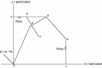
Note that if a technology satisfies strong disposability, it satisfies weak disposability also; however, the converse is not true (Färe et al., Reference Färe, Grosskopf, Noh and Weber2005). In figure 1, we illustrate how P(x) is constructed for a technology that satisfies the assumptions of weak and strong disposability. The line segment cd is a feasible part of the technology under the assumption of strong disposability of bad outputs since a movement from d to c would be possible without reducing any good output. The line segment ef represents the strong disposability of good outputs, while the segment de represents the best practice frontier, which is a convex combination of observed mixes of good and bad outputs. Thus, the output set bounded by the line segments 0cdef represents technology when there is strong disposability of bad outputs. If bad outputs are not freely disposable and resources have to be expended to clean up, then any reduction in bad output below the level observed at d requires either a reduction in the good output or an increase in the use of inputs if good output is not to be reduced. Both possibilities are costly; hence, disposal is not free. The output set is now represented by 0adef.
Output sets for strongly and weakly disposable bad outputs, and directional output distance function

A functional representation of the technology is provided by the directional output distance function, which also provides a measure of inefficiency. The directional distance function seeks to increase the good outputs whilst simultaneously reducing the bad outputs. Formally, the directional distance functionFootnote 6 is defined as

where g is the vector of directions in which outputs can be scaled. Following Chung et al. (Reference Chung, Färe and Grosskopf1997), the direction taken is g = (y, −b), such that as the good outputs are increased and the bad outputs are decreased.Footnote 7Figure 1 illustrates the directional output distance function for the direction vector g = (y, −b). A firm n, with output coordinates (y, b) produces inside the output set P(x)w. If it were to operate efficiently given the direction vector, g (represented by the ray 0g) it could expand y and contract b to be at the boundary of P(x)w at point a, under weak disposability conditions. Under strong disposability, it could expand y and contract b to be at point k on the boundary of P(x)s.
2.1. Environmental Efficiency (EE)
We assume that the directional output distance function is separable in good and bad outputsFootnote 8

where  . The set
 is a technology set restricted to the production of good outputs only without any consideration for undesirable outputs bt. Therefore, with this assumption one can decompose technical inefficiency into the factors that reflect the influence of ‘pure’ technical inefficiency,
 and the effect of undesirable outputs, B(bt). Thus, EE is defined as

EE will take values less than or equal to one. It represents the extent to which a country would be constrained in increasing outputs by its potential to transform its production process from free disposability to costly disposal of CO2 emissions. Countries that are less constrained have a lower opportunity cost of transformation in the production process and are considered to be more environmentally efficient. This measure takes a value one only for those countries which are on the segments de and ef or for those countries whose expansions fall on these segments (figure 1). Moreover, de and ef are common to both technologies with different assumptions on the disposability of bad outputs. For countries that lie on these segments, the cost of transforming the production process from strong disposability of bad outputs to weak disposability of these outputs would be zero. For countries located along the line segment 0ad, or in the interior part of the weakly disposable output set, the EE index will assume values less than one, indicating that there is an opportunity cost of transforming the production process from strong disposability to weak disposability of bad outputs.
2.2. Environmental Productivity (EP)
Following Färe et al. (Reference Färe, Grosskopf and Roos1995), the EP at time t + 1 using directional distance function is defined as

As explained above, we assume that the technology admits strong disposability of good outputs and weak disposability of bad outputs; so if b t+1 < bt,  and also
 . Hence, if less pollution is produced, the index value is greater than or equal to one, i.e. EP ≥ 1.
Chung et al. (Reference Chung, Färe and Grosskopf1997) define the Malmquist–Luenberger (ML) index between period t and t + 1 as

which can be further decomposed as

The first term, MLEFFCH, represents the efficiency change component, a movement towards the best practice frontier, while the second, MLTECH, the technical change.
In order to illustrate the relationship between the EP index (5) and the ML index (6) we note by introducing  and
 twice into (6) that

i.e. the ML index can be written as a product of the EP index and a measure of change in productivity for the given bad output vectors. We note that if the bad output vectors are dropped (using the assumption of separability between good and bad outputs), the term in the parentheses is the conventional measure of productivity (MS), i.e.

which can be further decomposed into two component measures of productivity change
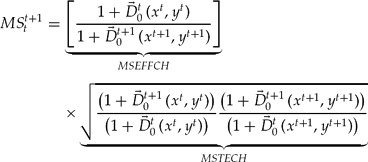
Furthermore, it is possible to decompose EP into environmental efficiency change (EEC) and environmental technological change (ETC) as follows

Thus, EP = EEC.ETC where EEC is environmental efficiency change and ETC is environmental technological change.
3. Empirical model
The distance function can be computed in various ways, but three are of particular interest: parametric linear programming (PLP) (e.g., Murty and Kumar, Reference Murty and Kumar2002; Färe et al., Reference Färe, Grosskopf, Noh and Weber2005), data envelopment analysis (DEA) (e.g., Färe et al., Reference Färe, Grosskopf, Lovell and Pasurka1989; Kumar, Reference Kumar2006), and econometric methods (e.g., Hetemaki, Reference Hetemaki1996; Kumar and Rao, Reference Kumar and Rao2003). There are two essential differences between the econometric approach and mathematical programming methods. The econometric approach is stochastic, and attempts to distinguish the effects of noise from the effects of inefficiency. Mathematical programming (parametric or non-parametric) is non-stochastic and lumps noise and inefficiency together. The parametric approaches confound the effects of misspecification of functional form (of both technology and inefficiency) with inefficiency. The DEA approach is non-parametric and less prone to this type of specification error.
We use DEA to compute the directional distance functions. The directional distance function for observation k' in period t, using period t technology can be calculated by solving the following LP problem.
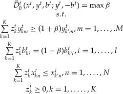
To measure the ML index, four DEA programs need to be solved for each observation. Two use observations and technology for time period t, or t + 1, and two use mixed periods using, for example, technology calculated from period t with the observation t + 1. Mixed period problems can cause difficulties in calculation, whereby the observed data in period t + 1 are not feasible in period t. For example, the observation (y t+ 1,k′, bt+ 1,k′) may not belong to the output set Pt(xt+ 1). To minimize this problem, we follow Färe et al. (Reference Färe, Grosskopf and Pasurka2001), whereby multiple year ‘windows’ of data are the reference technology. All frontiers are constructed from three years of data, hence the frontier for 1973, for example, would be constructed from data in 1973, 1972, and 1971, which reduces the likelihood of ‘non-solutions’.Footnote 9 Note that we compute a common frontier for all the countries included in this study using different disposability conditions with respect to bad outputs.Footnote 10
4. Data and discussion of results
We obtain data on five variables, GDP, CO2, labor force, capital stock, and commercial energy consumption, for 38 countries for the period 1971–1992. Out of these five, the first two variables, GDP and CO2, are considered as proxies for good and bad outputs respectively, and the remaining three are inputs into the production process. Data on GDP, labor force, and energy consumption are collected from the World Development Indicators (WDI) (World Bank), whereas the data on the CO2 emissions are obtained from the website of the World Resources Institute.Footnote 11 Capital stockFootnote 12 data are obtained from the Penn World Tables (Mark 5.6). GDP and capital stock are measured in 1985 US dollars, whereas CO2 and energy consumption are measured in thousand metric tons. The labor force data are in millions of employees. The 38 countriesFootnote 13 included here are those with data on capital stock and other variables over the period of 1971–1992. The choice of the period to be studied was also determined by the availability of capital stock data. Due to missing data for some countries for some years, we have 416 observations for annex-I countries and 405 observations for non-annex-I countries. Since EP is measured as a change in the levels of the distance function over two consecutive years, the number of observations available to analyze the determinants of EP is 19 less for each group of countries as compared to the observations available on EE.
Annex-I countries have higher GDP per capita, a higher share of industry and energy in GDP, and a larger openness index and a lower emission intensity of output measured by the ratio of CO2 emission to GDP. However, they have lower rates of growth of GDP, capital, labor, CO2, and energy consumption as compared to the non-annex-I countries. During the study period, non-annex-I countries not only had higher growth rates of income and emissions relative to annex-I countries, but there was also a higher degree of variability within this group. The newly industrialized country Hong Kong registered the highest growth rate of GDP (7.9 per cent) and it also had a high growth rate for CO2 emissions (6.5 per cent). Thailand experienced the second highest growth rate of GDP of 7.3 per cent but a more rapid rate of growth in the production of CO2, i.e. 8.3 per cent. The highest growth rate with respect to CO2 was in the Syrian Arab Republic (9.14 per cent). On the other hand, Sweden, France, Belgium, United Kingdom, and Denmark registered negative CO2 growth rates of 2.93, 1.71, 1.57, 0.66, and 0.32 per cent, respectively.Footnote 14
4.1. Estimates of directional output distance function
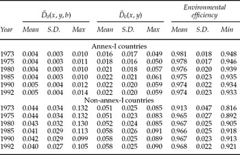
The directional output distance function is estimated with and without including CO2. This allows us to examine the importance of the inclusion of CO2 emissions in the analysis of efficiency and productivity changes. As described earlier the directional distance function provides a measure of technical inefficiency, the average values of this function for both models at certain points of time are presented in table 1.Footnote 15 We observe that the inefficiency scores when CO2 emissions are ignored are higher in comparison to the situation when this pollutant is weakly disposable. It reveals that the potential to increase the production of desirable output and reduce bad outputs with a given bundle of inputs is about 2.3 per cent.
Descriptive statistics of efficiency measures (geometric mean)

The group averages were constructed by pooling the data of annex-I and non-annex-I countries over the period, respectively. On average, the value of directional distance function for non-annex-I countries when CO2 emissions were included ranges from about zero for Paraguay to 0.087 for Nigeria, with mean value 0.055. This implies that 5.5 per cent of the GDP could have been increased and CO2 emissions could have been saved by improving efficiency and achieving the best practice frontier for these countries. For the annex-I countries this figure ranges between about zero for Japan to 0.057 for Canada. Under the weak disposability assumption the pooled average values of directional distance function over the period 1972–1992 for non-annex-I and annex-I countries are 0.042 and 0.005, respectively. The measure of inefficiency under weak disposability of CO2 can alternatively be interpreted as the extent to which there exist potentially win–win opportunities to reduce CO2 while increasing GDP given a country's distance from the best practice frontier facing it. This win–win opportunity is higher for non-annex-I countries than for annex-I countries (table 1).
4.2. Environmental efficiency of countries
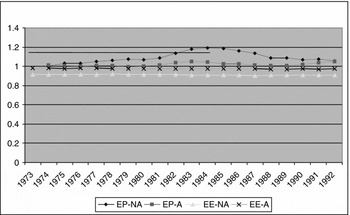
The estimates of EE are presented in table 1. Results for non-annex-I and annex-I countries show that on average the EE scores are 0.912 and 0.976, respectively, implying that, on average, these countries have an environmentally binding production technology. Under both disposability assumptions, inefficiency in the non-annex-I countries is higher in comparison to annex-I nations. In the non-annex-I group, countries with larger inefficiency differentials under the strong and weak disposability of CO2 assumption are Ecuador, Honduras, India, Kenya, Nigeria, Syrian Arab Republic, Zambia, and Zimbabwe. These countries have more environmentally binding production technology than others. Among the annex-I countries, there are only two countries that have non-binding production technology, i.e. Japan and Netherlands. We also find that the EE index on average is almost steady over the sample period in both the groups of countries (figure 2).
Environmental efficiency and productivity index
Note: EE-NA-I: EE Index for non-annex-I countries; EE-A-I: EE Index for annex-I countries; EP-NA-I: EP Index for non-annex-I countries; EP-A-I: EP Index for annex-I countries.

Countries with efficiency scores that differ under the assumption of weak disposability and strong disposability of CO2 suffer congestion from CO2 emissions, i.e. if these countries were to reduce emissions, they would have to sacrifice their GDP. Once this inefficiency is translated into loss of desirable output, the results indicate that developing countries like Ecuador, Honduras, India, Kenya, Nigeria, Syrian Arab Republic, Zambia, and Zimbabwe would have to lose more than 10 per cent of their GDP due to congestion of production technology. As a whole, countries in our sample would lose 5.6 per cent of GDP on average due to environmentally binding production technology. The relative output loss due to imposition of costly abatement for non-annex I countries is higher than the overall average of the entire sample.
4.3. Determinants of environmental efficiency
We now examine the factors that determine the changes in the EE index over time and the differences across countries. It is hypothesized that specific attributes of an individual country contribute to the environmental performance of that country. Using a Tobit model which recognizes the censored nature of the dependent variable, we examine the relationship between EE and its determinants by including variables such as GDP per capita, share of industrial output in GDP, the capital–labor ratio, energy intensity measured by the use of commercial energy per unit of GDP, population density, and openness index, defined as the ratio of total exports and imports to GDP. This measure of openness suffers from the limitation that it may combine the effects of ‘natural’ openness and the openness of the trade policy of a country. It may also depend on the level of development, distance from potential trading partners, country size, and factor endowments. Efforts to correct for these factors to determine effective openness and to control for trade policy effects also suffer from a number of drawbacks (Berg and Krueger, Reference Berg and Krueger2003). We include openness, as defined above, simply to control for the effect of actual trade openness (whatever its determinants) on environmental efficiency (as in Neumayer and Soysa, Reference Neumayer and de Soysa2005). The source of data on per capita GDP, share of industrial output, openness index and population density is the WDI.
The equation below specifies a possible form for the relation between the EE and the variables discussed above

where i is country index, t is time index, ϵ is the disturbance term such that ϵ ~ N(0, σϵ), GDPPC is GDP per capita, INDSHARE is share of industrial output in GDP, CAPLAB is capital per labor, ENGDP is use of commercial energy per unit of GDP, POPDENS is population density, OPEN is the openness index defined as the ratio of total exports and imports to GDP, Dt are the time dummies, and A is a dummy variable equal to 1 if a country belongs to the annex-I group.
The shape of the polynomial shows the relationship between EE and GDP per capita. It is expected that in the initial phases of industrialization EE would deteriorate but that it would show an improvement once a critical level of industrialization had been reached. This implies a quadratic relationship between EE and the share of industrial output in GDP, with the first-order coefficient being positive and the second-order coefficient being negative. A positive sign is expected for capital per labor variable if capital intensity leads to an increase in EE, otherwise it should be negative. A negative sign is expected for the ENGDP variable since it can be assumed that higher energy intensity of output leads to a decline in EE. The sign of the population density variable can be either positive or negative.Footnote 16 The openness variable could have either a positive or a negative sign depending on the way in which dependence on trade of a country affects EE. A negative sign could indicate that dependence on trade has environmentally deteriorating effects on EE. This could be the case if such countries seek to improve their competitiveness in the world market by using low cost but highly polluting technologies or if dirty industries migrate to the countries where environmental standards are weak. Trade liberalization might also encourage rapid extraction of natural resources and use of energy to produce and transport an increased volume of exports. On the other hand, a positive sign would suggest that trade has environmentally beneficial effects. These could arise due to easier access to cleaner inputs and technologies as well as greater availability of financial resources for environmental protection as the country grows. The sign and significance of the openness variable (and its quadratic term) will help selection among the competing hypotheses on the relationship between environment and international trade.
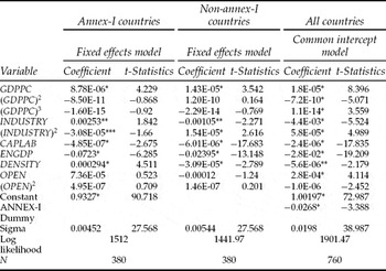
Table 2 provides the parameter estimates of the Tobit model for the EE index under alternative specifications. The choice between a fixed effects model and common intercept model is made using the log likelihood ratio test. We accept the null hypothesis that suggests the fixed effects model is the appropriate specification for each group of countries. In the case of joint sample, it is not possible to estimate a fixed effects model with a time invariant dummy for annex-I countries and hence for the joint sample we use common intercept model. In the joint sample model, we find that the group dummy variable, A-1, is statistically significant at the 1 per cent level. This implies that we should analyze these two groups of countries separately. The following discussion is therefore based on the group specific regressions.
Determinants of environmental efficiency (EE)

Note: *, **, and *** show the level of significance at 1%, 5%, and 10% respectively. Coefficients of time dummies are not reported to save space.
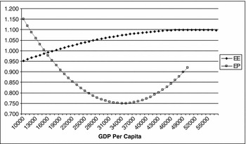
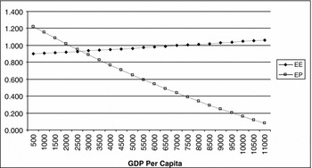
The most apparent outcome from the model based on the joint sample is that GDP per capita, its quadratic and cubic terms are statistically significant. However, for the group-specific models only, the first-order term is statistically significant. For the annex-I countries we find an increase in EE in the initial phases of growth (up to a per capita GDP level of approximately US$ 53,000) (figure 3) and then a phase of decline in EE. For the non-annex-I countries, we find a continuous increase in EE (figure 4) with respect to their observed per capita income. This implies that non-annex-I countries are adopting environmentally responsible technology much earlier (in terms of their GDP per capita) than annex-I countries.
EKC in EE and EP for Annex-I countries
Note: EE: environmental efficiency; EP: environmental productivity.

EKC in EE and EP for non-annex-I countries
Note: EE: environmental efficiency; EP: environmental productivity.

The effect of the share of industrial output in GDP on EE in the annex-I countries is inverted U-shaped. In non-annex-I countries, the observed shape of EE with respect to industrial share in GDP is U, the linear coefficient is negative, and the coefficient of the quadratic term is positive and both the coefficients are statistically significant. This indicates that in the initial phases of industrialization in these countries, EE declines, but as the process of industrialization deepens, EE improves.
Moreover, we find that the coefficient of POPDENS is consistently significant for both groups of countries, across all models; this variable is positively related to EE in annex-I countries and negatively for the other group. The coefficient of the energy intensity variable is negative and statistically significant for both groups, indicating that the increase in energy intensity leads to decrease in EE. An increase in capital per labor leads to decrease in EE in both groups.
Other variables that we included in the model are the index of openness and its quadratic term. We find that in the joint sample the coefficient of the linear term of openness index is positive, while the sign of the quadratic term is negative and both the coefficients are significant. This implies that for the sample countries, although trade is beneficial for the environment, deepening the openness of the economy leads to decrease in EE. However, for the individual groups neither of the coefficients of openness is statistically significant.
4.4. Environmental productivity of countries
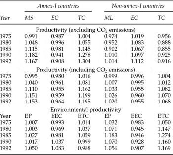
Measures of productivity change in each set of countries are presented in table 3 at an aggregate level and at five-year intervals. Recall that index values greater (less) than one denote improvements (deterioration) in the relevant performance.Footnote 17 Here we have calculated the Malmquist–Luenberger index and its components for both cases: including and ignoring CO2 emissions. Our method of computing productivity change utilizes a fixed base year (1973), and compares all subsequent years to that base.
Cumulative values of productivity indexes, and their components (1971 = 1)

Note: MS: Malmquist productivity index, ML: Malmquist-Luenberger productivity index, EC: Efficiency change, TC: Technological change, EEC: Environmental Efficiency Change, ETC: Environmental Technical Change, EP: Environmental Productivity.
The overall average of cumulative conventional productivity value that ignores the CO2 emissions had grown by about 9 per cent during the period 1973–1992. Moreover, the results show that the growth in productivity in annex-I countries was about 17 per cent and in non-annex countries its growth rate was only 1 per cent during the study period. Ecuador, Nigeria, Peru, Venezuela, Colombia, and Syrian Arab Republic experienced the highest decline in TFP among the developing countries. Hong Kong experienced the highest growth in MS among the non-annex-I countries. In the developed countries, Greece, Iceland, New Zealand, and Spain experienced the decline in productivity when the emissions of CO2 were ignored and the Netherlands experienced the highest growth rate in TFP.
Again we observe that most countries have lower growth in TFP when CO2 is considered an undesirable output in comparison to the conventional TFP growth. Kopp (Reference Kopp1998) finds that, between 1970 and 1990, developed countries experienced technical progress in a way that economizes on CO2 emissions but that developing countries did not. This variation in findings may be due to differences in estimation methods and in the group of countries considered developed and those that belong to annex-I. Among the non-annex-I countries, Hong Kong experienced the highest growth and Ecuador experienced the highest decline in TFP index. Among the annex-I countries, Belgium, Norway, France, Ireland, and Japan experienced the highest growth in environmentally sensitive TFP. Nevertheless, it was both technological and efficiency changes that governed the change in overall productivity indices in all countries.
Table 3 reports the cumulative value of EP index and its components at certain points for both of the groups. Figure 2 reveals that the growth in EP is almost equal over time in both of the groups. In non-annex-I countries, the index of EP varies from 0.60 to 1.43 and in annex-I it varies from 0.49 to 1.45. Thus, there was higher variability in EP index among developed countries in comparison to the developing ones. Moreover, the gap over time in EP remains almost constant between these two groups except during the mid eighties (figure 2).
4.5. Determinants of environmental productivity
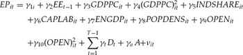
We hypothesize that the level of EP is determined by level of EE in the previous year, GDP per capita, capital per labor, share of industrial output in GDP, energy intensity, population density, and openness index. We examine the existence of an EKC type relationship between per capita income and EP as well as a relationship between EP and openness by estimating the following equation

where νit is the disturbance term. Table 4 provides the parameter estimates of the regressions for the EP index under alternative specifications. The log likelihood ratio test rejects the null hypothesis of a common intercept against the fixed/random effects model for both the groups of countries. However, for the regression of all the countries taken together we use a common intercept model for reasons stated above. The signs and significances of all coefficients are however robust across alternative models. We observe that most of the coefficients of time dummies are statistically insignificant. Similar to the model explaining variation in EE, we find that the country group dummy in the EP model that includes both groups of countries is statistically significant at the 5 per cent level. This suggests that we should use separate regression analyses to explain variations in EP in the two groups of countries.
Determinants of environmental productivity (EP)

Note: *, **, and *** show the level of significance at 1%, 5%, and 10% respectively. Coefficients of time dummies are not reported to save space.
For annex-I countries, we find that except for the coefficients for openness, all the other coefficients are statistically significant. Similarly, for non-annex-I countries, we find that except for openness and the linear term of industry variables, all the coefficients are statistically significant. The positive relationship between the environmental efficiency and environmental productivity index for the annex-I countries favors the existence of divergence hypothesis. However, for the non-annex countries we find the existence of convergence hypothesis, as the relationship between EE and EP is negative.Footnote 18 There is a positive relationship between capital per labor and EP for both the groups of countries, which implies that capital intensity leads to increase in EP. Furthermore, population density is negatively affecting EP in annex-I group.
We find that energy intensity contributes positively to EP in both the groups of countries. Similarly, we find that for the sample of all countries taken together energy intensity and EP are positively related. Since EP can be decomposed into environmental efficiency change and environmental technical change, the finding that energy intensity leads to decline in EE but an increase in EP implies that countries with higher energy intensity of their production processes are more likely to make environment friendly technological changes.
Of particular interest are the signs and significance of the coefficients of GDP per capita and its quadratic term and those of the openness index and its quadratic term. For annex-I countries the coefficients of GDP and its quadratic terms are statistically significant, and their signs imply the existence of an ‘U-shaped’ EKC type relationship for EP in these countries (figure 3). For non-annex-I countries, we observe that the linear term is negative and the quadratic term is positive, but both the terms are statistically insignificant (figure 4).
Moreover, the openness variable also exhibits an inverted U-shaped relationship between EP and openness for the joint sample. For the individual groups the sign of the linear and quadratic terms of the openness index are statistically insignificant. This implies that there is decline in environmental innovations up to a certain level of openness and then the environmental innovations start to improve once a critical threshold level is reached. The negative effect of international trade may be due to energy-related environmental damage such as carbon emissions that stem from increased transportation that is more pronounced below a threshold level of openness. However, as the degree of openness increases, this negative effect seems to be offset by the positive effects of harmonization of international environmental standards and technological transformations.
5. Conclusions
This paper estimates EE and EP indices using production frontier analysis, and compares them across countries and over time. The particular emphasis is on potential for transformation of production processes that allow free disposability of carbon emissions to costly disposal of these emissions to construct these indexes. As opposed to methods that measure the environmental quality with the levels of emissions of pollutants, the indexes that are derived in this study are based upon a production approach that differentiates between the disposability characteristics of the environmentally desirable and undesirable outputs.
EE and EP indexes are calculated using the non-parametric directional output distance function for two groups, annex-I and non-annex-I, each having 19 countries for the period of 1971 to 1992. On average, the world witnessed environmentally binding production technology during these two decades. The opportunity cost of the transformation of the production process from free to costly disposal of CO2 emission was about 5 per cent of GDP. The relative output loss due to imposition of costly disposal of CO2 emissions for non-annex-I group was higher than the average. The EE index was almost steady for the annex-I group, while its value is declining for the non-annex-I group over time.
TFP measures show that the progress witnessed by the world during the 1970s and 1980s was the combination of both factor accumulation and improvement in the productivity of factors of production. EP measured as the ratio of TFP under weak to strong disposability of CO2 emissions shows that it stagnated over time in both of the groups. However, there is high variability across countries over time.
A closer inspection of the EE index reveals that there was an improvement in EE in the initial phases of growth followed by a phase of decline in environmental quality once a critical level of per capita GDP was reached in the annex-I countries. This finding is similar in spirit to the results obtained in an EKC analysis. In the annex-I countries, the opportunity cost of the transformation of a production process from free to costly disposal of CO2 emission is becoming smaller after a certain threshold income level. But the non-annex-I countries are far behind in development in comparison to the annex-I countries, and the opportunity costs of transformation in production process are increasing. A closer inspection of these indexes reveals that after accounting for the effect of changes in the per capita income level on EE, there remains some variation in these indexes that can be explained by energy intensity, degree of industrialization, capital per labor, trade related variables, etc. We find in general that openness initially has a positive impact on EE but that this changes as openness increases, implying an inverted ‘U’ shaped relationship between EE and openness. However, we find a U-shaped relationship between EP and openness. This implies that initially trade liberalization negatively affects the environmental productivity of countries as they strive to compete in the world market but as they become more integrated in the world market, their environmental productivity improves. The results suggest that we must be careful in suggesting technological and managerial assistance to developing countries by the developed countries in increasing EE and EP in these countries apart from those associated with economic development.