

Introduction
Potato (Solanum tuberosum) is the third most important food crop in the world, after cereals and rice. Global production exceeds 300 million metric tons and is an important nutrition and calorie provider for humanity (Pareek Reference Pareek2016). Potato production is threatened by several diseases resulting in considerable yield losses, and causing decrease in the quality and increase in the price of potatoes (Taylor et al., Reference Taylor, Pasche and Gudmestad2008). An early disease detection system can aid in avoiding such cases. Moreover, it can improve the management of the crop and can further prevent the spread of diseases (Rich Reference Rich2013). Manually detecting and sorting potatoes is difficult, costly, and time consuming, while computerized inspection may be more efficient and cost effective.
Computer vision and machine learning techniques for disease detection have been broadly researched in the last two decades (Garcia and Barbedo Reference Garcia and Barbedo2016). Diseases can be detected using expensive and bulky digital imaging sensors, such as spectral or near-infrared sensors. Using such sensors encumbers the widespread implementation of these methods due to its high costs and maintenance (Sankaran et al., Reference Sankaran, Mishra, Ehsani and Davis2010). On the other hand, researchers using the visible light bandwidth, which can be captured by relatively low cost cameras, have usually focused on a single type of disease (Zhang et al., Reference Zhang, Huang, Jiangbo, Zhao, Fan, Wu and Liu2014). A single case identification is insufficient for real-world applications, as a single tuber can be infected a number of diseases (Cubero et al., Reference Cubero, Lee, Aleixos, Albert and Blasco2016).
This paper leverages recent advances in computer vision and object recognition, for classifying multiple diseases in potatoes. In 2012 a group of researchers from Toronto won the Large Scale Visual Recognition Challenge (ILSVRC) competition by improving the classification of the ImageNet database by more than 10%. They achieved a top-5 error rate of 15.3% when using a deep Convolution Neural Network (CNN), while the second best achieved 26.2% error rate (Krizhevsky, Sutskever, & Hinton, Reference Krizhevsky, Sutskever and Hinton2012). Since then, CNN methods have improved and recently the classification error dropped to 3.73% by the winning team for the same task (Abdi and Nahavandi Reference Masoud and Nahavandi2016). In the field of computer vision for agricultural applications, the use of CNNs and other deep neural networks is continuously increasing (Gongal et al., Reference Gongal, Amatya, Karkee, Zhang and Lewis2015). A CNN was recently used for detecting and classifying seven fruits in field conditions, improving detection accuracy by 3% from the last state of the art (Sa et al., Reference Sa, Ge, Dayoub, Upcroft, Perez and McCool2016). CNNs used in classification tasks, such as disease classification of plant leaves or quality control of harvested fruit and vegetable, reached accuracy of more than 97% (Mohanty et al., Reference Mohanty, Hughes and Salathé2016; Tan et al., 2015). In order to create successful CNNs, a large amount of training data is needed (Sermanet et al., Reference Sermanet, Eigen, Zhang, Mathieu, Fergus and LeCun2013). Therefore, the first aim of the current research was the collection of a sufficient dataset and classification of the displayed diseases. Results indicate a first step towards multiple disease classification for potatoes using CNN.
Materials and Methods
Data acquisition
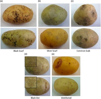
Photos of 400 contaminated potatoes of different shapes, sizes and tones were acquired under normal uncontrolled illumination conditions. The tubers were manually classified by experts as a standard procedure of statistically estimating the rate of various diseases in seed potato tubers prior to planting them in the fields. This procedure is done annually independent of the current research. The potatoes were contaminated with four different diseases, all with significant visual symptoms on the tuber’s skin (see Figure 1). The images were acquired using multiple types of standard cameras, captured from one viewpoint only. The cameras used were Sony DSC-T200, the Apple iPhone 4 camera, and the Samsung Galaxy S3 camera.
Examples of visual symptoms on potato diseases: (a) Black Scurf disease - irregular, black, scab-like marks on the skin of the tuber. (b) Silver Scurf disease - circular or irregular, tan to silvery gray lesions on the tuber’s skin. (c) Common Scab disease - circular brown rough areas, with irregular margins which can coalesce into larger areas. (d) Black Dot disease - tiny black dots on the skin of the tuber (magnified in top left corner). (5) Uninfected tuber.

Data preparation
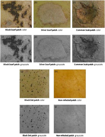
The images acquired were used to create the training and tests sets for the CNN. Every visual symptom of a disease was marked and labelled using the image labeler application in MatLab 2014b. The labelling was done with rectangular bounding boxes encompassing the visual symptom but also much regular potato skin, as seen in Figure 2. The marked areas were cropped from the original image, transformed into grayscale, and resized to a standard 224×224 pixel square. After preprocessing, a total of 2,465 patches of diseased potatoes was gathered including: 265 Black Dot patches, 469 Black Scurf patches, 686 Common Scab patches, 738 Silver Scurf patches and 307 uninfected patches.
Examples of diseased potato patches before and after the transformation to grayscale. (a)–(c), (g) and (h) are the original RGB images from each class. (d)-(f), (i) and (j) are the same images after the conversion to grayscale, using Matlab’s rgb2gray function.

Performance Measurement
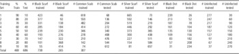
The experiment was designed to evaluate the performance of the CNN’s learning algorithm in classifying four diseases and uninfected potatoes. As manually labelling diseased patches of potatoes is a tedious and time costly task, an important task was to determine the minimal amount of training data that provides sufficient classification accuracy. The CNN was trained with different sizes of training sets. The smallest training set used for training was 10% of the 2,465 images, incrementally increasing by 10% to 90% of the whole dataset as detailed in Table 1. In each increment the images were selected uniformly from the whole dataset. Testing of the algorithm was done on the remaining data. In total the training and testing phases was repeated 9 times over different training set sizes.
Train and test set division.

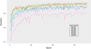
Each training set was trained for 90 epochs, where one epoch is defined as a one full training cycle on every sample in the training set. The choice of limiting to 90 epochs was made based on empirical observations that revealed that the learning converged well within 90 epochs (as can be seen in Figure 4). In order to compare between the different results over the 9 training sets, the error rate of the best scoring guess was calculated as the number of errors divided by the total number of test images in every epoch. The error was calculated both for test and train sets, in order to understand the over\under fitting of the procedure.
Algorithm
The algorithm chosen for the image classification task was a deep convolutional neural network (CNN). The basic architecture chosen for this problem was a CNN developed by the Visual Geometry Group (VGG) from the University of Oxford named CNN-F due to its faster training time (Chatfield et al., Reference Chatfield, Simonyan, Vedaldi and Zisserman2014). Several new dropout layers were added to the VGG architecture to deal with problems of over fitting, especially due to the relatively small dataset.
The required input image size for this network is a 224×224 matrix. The CNN comprises 8 learnable layers, the first 5 of which are convolutional, followed by 3 fully-connected layers and ending with a softmax layer (see Figure 3). The softmax layer normalizes the input received from the last fully-connected layer (fc3) producing a distribution of values, one for each class. The sum of these values add up to 1 and they represent the probability of the input image to belong to one of the five classes. This softmax layer was also altered and adapted, reducing its size from 1,000 to 5 to fit our classification task.
A simplified model of the CNN used.

The hyper-parameters used in each training experiment were:
-
∙ Solver type: Stochastic Gradient Descent
-
∙ Learning rate: 0.0001
-
∙ Batch size: 50
-
∙ Momentum: 0.9
-
∙ Weight decay: 0.0005
Training CNNs usually requires a large amount of labelled data in order to perform a good classification. Therefore, two methods were used for data augmentation; Mirroring creates additional examples by flipping the images used in training randomly. As the direction of the photos was arbitrary, mirroring the image horizontally does not change the correctness of the data; Cropping was also used, cropping the image randomly to different sizes, while keeping the cropped image minimum size to 190×190, can achieve data diversity. The use of each data augmentation method was done randomly. Before each image was inserted into the net for training it was mirrored, cropped or inserted without altering in equal distributions. Therefore, two thirds of the images trained were altered.
Results and discussion
Results indicate, as expected, that using more data for the training phase improves the classification and reduces the error rate (see Figure 4). The best trained model (trained on 90% of the dataset and tested on the remaining 10%) classified correctly 96% of the images. Results indicate that for 8 out of the 9 training sets, accuracy does not drop below 90% as the training set size decreases (Figure 4); the average difference of error rates between the best training set (90% train-10% test) and the worst training set (20% train-80% test) in these 8 sets was 5.73%. There is a significant drop in performance when the CNN was trained on 10% of the dataset and tested on 90% of it. Correct classification for this training set decreased to 83% as opposed to 90% of the classifier obtained with 20% train and 80% test. The relatively small decrease in accuracy (Table 2) for most training set sizes, is an indicator that a small amount of potato images could suffice for training a sufficiently accurate CNN.
Results of the experiment. Top plot shows the accuracy of each training set (colored and dotted graphs) according to the epoch number. The bottom plot show the smoothed results.

Best performing model accuracy results for each train-test set

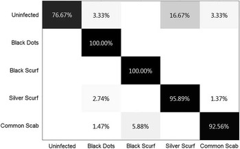
In order to further evaluate the CNN’s classification a confusion matrix was calculated. The confusion matrix’s columns represent the CNN’s class classification while the rows represent the actual classes. This type of representation can help evaluate the CNN’s classification of each class. Figure 5 shows a confusion matrix of the best performing CNN, trained on 90% of the dataset and tested on 10%. The confusion matrix shows that the CNN classified correctly and with high accuracy infected potato tubers; 100% of the tubers which were infected with Black Dot and Black Scurf were classified correctly; over 92% of the Silver Scurf and Common Scab infected tubers were classified correctly as well. The CNN’s performance dropped when classifying uninfected tubers. Most of the CNN’s misclassifications occurred when classifying uninfected tubers to the disease class – Silver Scurf. Silver Scurf’s visual symptom are bright tan to silvery gray lesions on the tuber’s skin that resemble uninfected skin.
A confusion matrix of the CNN trained on 90% of the dataset and tested on the remaining 10%. Rows represent the actual classes of an image. Columns represent the CNN’s class prediction. Each cell in the matrix represent the percentage of images of the row’s class that were classified to the column’s class.

These results indicate that the trained CNN can classify correctly and accurately the four diseases presented here. However, uninfected tubers were harder to classify. The fact that the diseases were classified with high accuracy makes it suitable for a system which identification of the disease is important. Most misclassifications occurred for the uninfected class, for practical use these mistakes have less affect since planting infected tubers can spread the disease and cause considerable damage while misclassifying uninfected tubers can be solved. In this experiment only 307 images of uninfected tubers were used, increasing the amount of data of uninfected tubers can increase classification accuracy.
Conclusions and future work
The applicability of a convolution neural network in classifying image patches of diseased potatoes into four disease classes and a uninfected class was examined. The 2,465 images classified by the trained CNN model varied in the acquisition device and conditions. Results indicate the robustness of the classification algorithm allowing for uncontrolled acquisition conditions. Results reveal that the correct classification of fully trained CNN models ranges from 83% for the model trained on the least amount of data, to 96%, when the model was trained on 90% of the data. To obtain classification rates higher than 90% it is sufficient to use 20% of the images (i.e., 493 images).
These results further show that combining the CNN introduced here with a sliding window algorithm could be utilized for classifying full images of potatoes to different diseases with little labelling work beforehand. Ongoing research is aimed to develop a classification algorithm with an expanded number of disease classes. Acquiring data can be done easily since there are no constraints on the data acquisition.
Acknowledgements
This work is supported by the Ministry of Agriculture and partially supported by the Helmsley Charitable Trust through the Agricultural, Biological and Cognitive Robotics Initiative and the Rabbi W. Gunther Plaut Chair in Manufacturing Engineering, both at Ben-Gurion University of the Negev. We thank Professor Yael Edan for her important comments.