2. Formulation, roughness configuration and data processing

The Navier–Stokes and continuity equations read as

(2.1) \begin{align} \frac {\partial u_i}{\partial t} + \frac {\partial u_i u_{\kern-1pt j}}{\partial x_{\kern-1pt j}} = -\frac {1}{\rho } \frac {d \overline {p}}{dx} \delta _{i1} -\frac {1}{\rho } \frac {\partial p}{\partial x_i} + \nu \frac {\partial ^2 u_i}{\partial x_{\kern-1pt j} \partial x_{\kern-1pt j}} , \\[-28pt] \nonumber \end{align}

(2.2) \begin{align} \frac {\partial u_k}{\partial x_k} = 0, \\[-2pt] \nonumber \end{align}

where $\nu$ is the kinematic viscosity, $\rho$ is the fluid density, $x_i$ (or equivalently $x$ , $y$ and  $z$ ) denotes the streamwise, wall-normal and spanwise directions for $i=1,2\,\text{and}\,3$ , $u_1$ , $u_2$ and $u_3$ (also denoted by $u,\,v \,\text{and}\,w$ ) stand for the streamwise, wall-normal and spanwise velocity components, respectively, and $\delta _{\textit{ij}}$ is the Kronecker delta. The quantity $- ({{\rm d}\overline {p}}/{{\rm d}x})$ is the overall imposed streamwise pressure gradient, which is maintained constant. The flow rate, and consequently the bulk velocity $\langle \overline {U} \rangle _b= {1}/{H} \int _{0}^{H} \langle \overline {U} \rangle {\rm d}y$ , where, $H$ is the half-channel width, changes in time before the bulk Reynolds number $ \textit{Re}_{b}=H \langle \overline {U} \rangle _b/\nu$ reaches a steady state, as in Coceal et al. (Reference Coceal, Thomas, Castro and Belcher2006). The shear velocity is $\overline {u}_\tau =\sqrt { {(-H{\rm d}\overline {p}/{\rm d}x})/{\rho }}$ . The friction Reynolds (Kármán) number is particularly low and it is kept constant at $ \textit{Re}_\tau =H\overline {u}_\tau /\nu =125$ in all of the cases.

The passive scalar problem is investigated in a way similar to Lyons, Hanratty & McLaughlin (Reference Lyons, Hanratty and McLaughlin1991). The temperature is held constant over the lower rough wall at $T_l=-T_w$ and at $T_u=T_w$ at the upper rough wall, as in Leonardi et al. (Reference Leonardi, Orlandi, Djenidi and Antonia2015). Here, $\Delta T$ denotes $\Delta T=T_u-T_l$ and $\theta =T-T_l$ . The equation for $\theta$ reads for

(2.3) \begin{align} \frac {\partial \theta }{\partial t} + \frac {\partial u_k\theta }{\partial x_k} = \alpha \frac {\partial ^2 \theta }{\partial x_k\partial x_k}, \end{align}

where, $\alpha$ is the diffusivity. The Prandtl number is chosen as $ \textit{Pr}=\nu /\alpha =1$ to emphasise the similarity or dissimilarity between the passive scalar and velocity fields. No-slip conditions are used for the velocity field. This is combined with periodic boundary conditions in the streamwise and spanwise directions. Hereafter, $ ( )^*$ denotes quantities normalised by $H$ , and the bulk velocity $\langle \overline {U}_b\rangle$ . The wall temperature is defined as $\overline {T}_\tau = [ ( {\partial \langle \overline {T} \rangle }/{\partial y^*} )_{y^*} ]/ \textit{PrRe}_\tau$ , where $ ( {\partial \langle \overline {T} \rangle }/{\partial y^*} )_{y^{*}}$ is the average at $y^*=0$ between the roughness elements and $y^*=k^*$ over the crests, where it is recalled that $k$ stands for the height of the roughness elements. It is found that $\overline {T}_{\tau }$ changes very little from one roughness configuration to another. The inner scaling $ ( )^+$ refers to the normalisation by the inner variables $\overline {u}_\tau$ , $\overline {T}_\tau$ and $\nu$ . The former is based on the overall $-({\rm d}\overline {p}/{\rm d}x)$ . Scaling based on the local shear velocity $u_{\tau ,l}$ will be denoted by $ ( )_+$ , as will be indicated again in the manuscript when the time comes.

The momentum and passive scalar equations are coupled with the immersed boundary method (IBM) described in Fadlun et al. (Reference Fadlun, Verzicco, Orlandi and Mohd-Yusof2000) in the DNS performed here. The direct forcing technique of Kim, Kim & Choi (Reference Kim, Kim and Choi2001) is used for the velocity field, while the interpolation technique of Fadlun et al. (Reference Fadlun, Verzicco, Orlandi and Mohd-Yusof2000) is used for the temperature field. The time advancement is performed using a third-order Runge–Kutta scheme. Second-order explicit optimised schemes combined with a structured Cartesian grid that is homogeneous in the streamwise and in the spanwise directions and non-homogeneous along the wall-normal direction, enabling a refinement near the walls, are used. More details on the DNS can be found in Bauer, Tardu & Doche (Reference Bauer, Tardu and Doche2015).

The roughness elements covering both the lower and upper walls are square bars of large height $k^*=k/H=0.27$ corresponding in wall units to $k^+=34$ . The roughness geometry is shown in figure 1. The staggering parameter characterising the streamwise shift between the roughness elements is denoted by $s^*$ . The latter is varied from $s^*=0$ (transverse bars spanning the whole channel width) to $s^*=12k^*$ in the six distinct cases investigated so far. Only significant results will be presented here. There is an infinite number of configurations resulting from different combinations of the roughness distribution characteristics. In an attempt to design a somewhat academic case, we chose geometrically similar configurations by referring to similar rectangles of sides $(s^*,p^*)$ . The pitch is, therefore, chosen as $p^*/s^*=\text{constant}=2$ in all of the cases.

The IBM method requires fine meshes near the roughness elements. This is why the streamwise and spanwise mesh sizes are as fine as $\Delta x^+=0.8$ and $\Delta z^+=3$ here. The wall-normal resolution between the roughness elements varies from $\Delta y^+=0.24$ at the wall to $\Delta y^+=2.76$ at the centreline. The spatial extents of the computational domain in outer scales and the number of computational modes are provided in table 1. It is seen that the streamwise length $L_x$ varies between $10H$ and $20H$ which is an order of magnitude larger than in Leonardi & Castro (Reference Leonardi and Castro2010), who investigated a turbulent channel flow over large cube roughness. The reason why we changed the streamwise length of the computational domain in some configurations will later be given. The computations for all the cases started with the same uniform velocity and had start up periods denoted by $\Delta T_{\textit{St}}$ at the end of which $\textit{Re}_b$ reached a steady state. These periods are non-dimensionalised by the outer time scale $H/\langle \overline {U}_b \rangle$ (table 1). Subsequently, the time elapse during which the averaging process is performed is denoted by $\Delta T_{Av}$ . The averaging time used here is $1400\leqslant \Delta T^*_{Av}\leqslant 2200$ and is roughly six times larger than in Leonardi & Castro (Reference Leonardi and Castro2010). For comparison purposes, DNS of a fully developed turbulent channel flow over smooth walls at $\textit{Re}_\tau =125$ are conducted in parallel in a computational domain of size $L_x^*\times L_y^*\times L_z^*=12\pi \times 2\times 4\pi$ , using $768\times 128\times 386$ computational nodes leading to $\Delta x^+=7.3$ and $\Delta z^+=4.9$ . The statistics in the smooth channel are obtained by averaging 40 statistically independent flow fields.

Table 1.

Flow conditions and computational details. The configurations are denoted as $s\beta p\gamma$ , where $\beta =s^*/k^*$ and $\gamma =p^*/k^*=2s^*/k^*$ (figure 1). See the text for further details.

Figure 1.

Schematic of a segment of the staggered roughness configuration (a) and top view of the roughness distribution and its parameters (b). The flow is along the streamwise direction $x$ . The shift between two consecutive staggered roughness elements is denoted by $s^*=s/H$ , the separation between two aligned square bars is $p^*=2s^*$ . The height and the side of the roughness elements are fixed at $k^*=0.27$ .

Note in table 1 that $\textit{Re}_b$ is particularly low in this investigation. The bulk Reynolds number is even below the subcritical limit $\textit{Re}_{\textit{bsc}}\approx 700$ when $s^*/k^*\leqslant 6$ . The subcritical limit is defined as the critical Reynolds number for substantial three-dimensional growth of moderate two-dimensional disturbances (Orszag & Patera Reference Orszag and Patera1983). The bulk Reynolds number is comparable to $\textit{Re}_{\textit{bsc}}$ in the case $s^*/k^*\geqslant 9$ . We will distinguish hereafter the configurations between the small shifts $s^*/k^*\leqslant 3$ and the large shifts $s^*/k^*\geqslant 9$ . These cases will be denoted by SS and LS, respectively. The case $s^*/k^*=6$ at which $\textit{Re}_b=419$ is lowest is an intermediary configuration for reasons that will be clarified later. The reader is invited to keep in mind that the Reynolds number is below the subcritical limit in SS, while $\textit{Re}_b\approx \textit{Re}_{\textit{bsc}}$ in LS.

The inhomogeneity near the roughness elements in the $x{-}z$ planes can explicitly be taken into account by using the triple decomposition (Nikora et al. Reference Nikora, McLean, Coleman, Pokrajac, McEwan, Campbell, Aberle, Clunie and Koll2007; Hantsis & Piomelli Reference Hantsis and Piomelli2022). The latter is a mixture of spatial and temporal averages of a flow quantity $q(x_i;t)$ which is decomposed as

(2.4) \begin{align} q(x,y,z;t) = \overline {q}(x,y,z)+q^\prime (x,y,z;t)=\langle \overline {q}\rangle (y) + \tilde {q}(x,y,z) + q^\prime (x,y,z;t). \end{align}

Here, $\overline {q}$ is the time-averaged flow quantity, spatial averaging is denoted by the angled brackets, so that $\langle q\rangle$ denotes the spatial average in the $x{-}z$ planes of the temporal mean, $\tilde {q}$ is called the wake field, and it quantifies the spatial variations of the temporal mean $\langle \overline {q} \rangle$ i.e. the dispersive effects induced by the roughness elements. Thus $\overline {q}=\langle \overline {q}\rangle +\tilde {q}$ . Obviously, $\langle \tilde {q}\rangle =0$ . The form-induced perturbation is zero in a flow homogeneous in the $x{-}z$ planes, such as for example, in the region far from the roughness elements or over a smooth wall. In such a case, the triple decomposition becomes equivalent to the classical Reynolds decomposition. Plane averaging of the time-averaged quantities is performed over the area occupied by the fluid, as in Peeters & Sandham (Reference Peeters and Sandham2019). This is labelled as the intrinsic spatial average in Mignot, Barthelemy & Hurther (Reference Mignot, Barthelemy and Hurther2009).

Figure 2.

Comparison of the turbulent shear stresses $(a)$ , with the streamwise turbulent intensity $\overline {u'u'}^+$ (blue), the wall-normal intensity $\overline {v'v'}^+$ (orange) and the spanwise turbulent intensity $\overline {w'w'}^+$ (green), and of the Reynolds shear stress distributions $(b)$ with the lattice Boltzmann method (LBM) results of Anika et al. (Reference Anika, Djenidi and Tardu2020) for the case $s^*=9k^*$ . Symbols: DNS results obtained in this investigation. Solid lines: Anika et al. (Reference Anika, Djenidi and Tardu2020). The results are obtained through the conventional Reynolds averaging above the crests. The bulk Reynolds number is $\textit{Re}_b=675$ in DNS, while $\textit{Re}_b=880$ in the LBM simulations. The origin $y^*=0$ is the base wall in $(a)$ and it is taken at the roughness crest plane in $(b)$ .

The configuration $s^*=9k^*$ is identical to Anika et al. (Reference Anika, Djenidi and Tardu2020) who used numerical simulations based on the LBM. The DNS results obtained here are in close agreement with these authors, as a whole (Arrondeau Reference Arrondeau2023). Figure 2 compares, for instance, the turbulent shear stress and the Reynolds shear stress profiles obtained by DNS in this investigation, with the LBM results of Anika et al. (Reference Anika, Djenidi and Tardu2020). It is seen that there is a close agreement with these authors both qualitatively and quantitatively despite the slight differences in the bulk Reynolds number, which is $ \textit{Re}_b=675$ here (table 1) against $ \textit{Re}_b=880$ in the LBM simulations. The resolution near the wall is sub-Kolmogorov here, while it is limited to $\varDelta ^+=2$ in LBM. These results are obtained through the conventional Reynolds averaging over the crests as in Anika et al. (Reference Anika, Djenidi and Tardu2020) who did not process the data through the triple decomposition and double averaging.

Figure 3.

Contribution of the viscous (closed circles) and form drags (closed triangles) denoted respectively by $D_\nu /Dt_{\textit{tot}}$ and $D_f/Dt_{\textit{tot}}$ . $(a)$ Repartition for different shifts $s^*/k^*$ , $(b)$ repartition for different plan area densities $\lambda _p$ .

Figure 3 $(a)$ shows the contributions of the viscous and form drags, denoted respectively by $D_\nu /D_{\textit{tot}}$ and $D_f/D_{\textit{tot}}$ , for different $s^*/k^*$ , where $D_{\textit{tot}}$ stands for the total drag $D_{\textit{tot}}=D_\nu +D_f$ . The results are shown as the function of the plan area density $\lambda _p$ of the roughness distribution in figure 3 $(b)$ . The plan area density $\lambda _p$ is defined as the plan area of the square bars divided by the total plan area. Because the roughness elements are square bars, the plan area and the frontal area densities are the same. Here, the larger $\lambda _p$ the smaller the shift $s^*/\kappa ^*$ . It is seen in figure 3 that the form drag dominates and that it is the main contributor to the total drag. It is interesting to note that $D_\nu /D_{tot}$ has a minimum at $\lambda _p\approx 0.15$ corresponding to $s^*/\kappa ^*=3$ . The same behaviour was reported in Leonardi & Castro (Reference Leonardi and Castro2010) (their figure 7 $a$ ) at the same $\lambda _p$ although the large cube roughness these authors have investigated is a totally different morphology, so that this could be coincidental. The subsequent increase of $D_\nu$ following the local minimum is attributed to the recirculating regions between the cubes in Leonardi & Castro (Reference Leonardi and Castro2010). We will show later that the viscous drag increase at the largest $\lambda _p=0.2$ $(s^*/\kappa ^*=2)$ is due to the large contribution of the crest friction (figure 17 $b$ ) and the differences in the flow topology characteristics compared with large-shift cases (figure 4).

3. Set-up of three-dimensionality

Figure 4.

$(a)$ Root-mean-square (r.m.s.) of turbulent intensities of the streamwise $u'_{\textit{rms}}$ , wall-normal $v'_{\textit{rms}}$ and spanwise $w'_{\textit{rms}}$ velocity components in wall units in an initially laminar channel flow with square bars spanning the whole transverse width $(s^*/k^*=0)$ . It is seen that $w'_{\textit{rms}}$ is strictly zero in the entire channel, $(b)$ large temperature oscillations and of the associated flow field observed across the channel when $s^*/k^*=0$ and $(c)$ set-up of three-dimensionality with regeneration of coherent eddies induced by the roughness elements in the configuration with small shift $s^*/k^*=2$ . The coherent eddies are detected by the $\lambda _2$ technique (Jeong et al. Reference Jeong, Hussain, Schoppa and Kim1997). They are shown by the $\lambda _2^+=-0.02$ contours and coloured by their distance normal to the wall. Red tones mark large wall-normal distances.

It has to be recalled that the flow is initially laminar and two-dimensional (2-D). To be clear, there is no background turbulence or noise added to the initial velocity field, and the by-pass transition is triggered (or not) by the roughness elements alone. It is found that it remains two-dimensional when transverse square bars span the whole width of the channel, i.e. when the shift parameter is $s^*=0$ . Under these circumstances, the flow consists of secondary motions in the canopies and the instantaneous local spanwise velocity component is zero; thus $w'(x,y,z,t)= 0$ (figure 4 $a$ ). These results are in close agreement with Anika et al. (Reference Anika, Djenidi and Tardu2018). Figure 4 $(b)$ shows the streamlines and the instantaneous contours of the temperature field at $s^*=0$ . It is seen that strong oscillations of the streamwise and wall-normal velocity field are accompanied by large local temperature variations. This case alone is interesting, and some key elements that have already been discussed in detail in Anika et al. (Reference Anika, Djenidi and Tardu2018) are briefly summarised here. In the absence of the local spanwise velocity component, the major production term in the instantaneous transport equation $ {D \omega _x}/{Dt}$ of the local streamwise vorticity (Brooke & Hanratty Reference Brooke and Hanratty1993), namely the tilting of the wall-normal vorticity by the mean shear that reduces to $-( {\partial w'}/{\partial x})( {\partial \overline {U}}/{\partial y})$ , is missing. This term is responsible for the generation of intense $\omega _x$ layers that roll-up into the Reynolds shear stress, producing eddies in the low buffer layer in the canonical wall turbulence (Tardu Reference Tardu2022). Therefore, breaking up of the spanwise symmetry is necessary to generate local $w'$ and $-\partial w'/\partial x$ that, in return, can feed the velocity–pressure gradient term $\varPi _{w'w'}=- ({2}/{\rho })\langle \overline {w'({\partial p'}/{\partial z}}) \rangle$ allowing the inter-component transport $\langle \overline {u'u'} \rangle \rightarrow \langle \overline {w'w'} \rangle$ to be set up (Tardu Reference Tardu2014). The spanwise symmetry is broken up by spanwise asymmetric pulsed wall jets in Anika et al. (Reference Anika, Djenidi and Tardu2018) to trigger $w'$ . In the passive by-pass transition mechanism investigated here, a small shift $s^*$ between the roughness elements is large enough to break-up the spanwise symmetry and trigger the 3-D turbulent field. Figure 4 $(c)$ shows the structures depicted by the $\lambda _2$ technique (Jeong et al. Reference Jeong, Hussain, Schoppa and Kim1997) in the case $s^*=2k^*$ for which the shift $s^*$ is nearly five times smaller than in Anika et al. (Reference Anika, Djenidi and Tardu2020). The structures are the $\lambda _2^+\leqslant -0.02$ isosurfaces and they will shortly be denoted by $\lambda _2^+=-0.02$ events in the manuscript. Hereafter, and except where specifically indicated, the threshold in this detection scheme is fixed at this value. Note that the vortical structures regenerate in their great majority at the edges of the square bars and within the small gaps in between, wherein the $-\partial w'/\partial x$ shear layers are primarily set up. We will discuss these points in more details later.

4. Mean velocity and temperature distributions

Figure 5.

$(a)$ Mean velocity profiles in wall units versus the wall-normal distance, $(b)$ velocity defect profiles and $(c)$ mean temperature distribution in wall units. The solid black line corresponds to the fully developed turbulent flow in a smooth channel at $ \textit{Re}_\tau =125$ . See the text for details.

The mean velocity profiles $\langle \overline {U}\rangle ^+$ are shown in figure 5 $(a)$ . Hereafter, the origin $y^*=0$ is the base wall. The solid black lines correspond to the DNS data obtained in a fully developed turbulent smooth channel flow at $ \textit{Re}_\tau =125$ . It is interesting to note in figure 5 $(a)$ that the $\langle \overline {U}\rangle ^+$ distributions are similar, with an apparent logarithmic region with the same slope as in the smooth channel in all the cases. Recall that the Reynolds number is low and the roughness elements are high, so that the extent of the apparent log layer is restricted to a narrow region of a few dozen wall units above the crests. Thus, there is no clear separation between the inner and outer scales, so that the basic von Kármán hypotheses are not fulfilled in the smooth nor the rough channels at this particularly low Reynolds number $ \textit{Re}_\tau =125$ . The reader can refer to Tardu (Reference Tardu2014) for a review on these aspects, including some relevant references. The broken blue line in figure 5 $(a)$ stands for the logarithmic velocity profile $\langle \overline {U}\rangle ^+ = {1}/{\kappa }\,\,\text{ln}(y^+)+B$ , with $\kappa =0.4$ . The downward shift $\Delta U^+ = \overline {U}^+_s - \langle U \rangle ^+_r$ where the sub-indices $r$ and $s$ refer, respectively, to the rough and smooth channels, decreases with increasing $s^*$ . The roughness function $\Delta U^+$ in a sufficiently large Reynolds number fully rough turbulent flow is defined in the log layer. Thus, the downward shift is shown at $y^+=70$ in figure 5 $(a)$ , assuming that this wall-normal position is presumably within the pseudo-logarithmic layer. Given the ensemble of the restrictions due to low Reynolds number effects and to the particularly large heights of the roughness elements, $\Delta U^+$ can be analysed only on a qualitative basis. The large values of $\Delta U^+$ noted in figure 5 $(a)$ reflect the large values of the form drag in concordance with figure 3. Some flow quantities behave as they were in the fully rough regime in all of the configurations and the velocity roughness function increases monotonically, as with the form-induced drag. Recall inter alia that the flow is usually characterised as fully rough when the form drag dominates the friction drag, as is the case in figure 3. For the ensemble of these arguments, and despite the particularly low Kármán number $ \textit{Re}_\tau =125$ investigated here, the regime will be labelled as fully rough hereafter. The reader should, however, keep in mind all the reservations that have just been mentioned above on this matter.

Figure 5 $(b)$ shows the mean velocity defect $\langle \overline {U}_c\rangle ^+ - \langle \overline {U}\rangle ^+$ as a function of $y^*=y/H$ , where $\langle \overline {U}_c\rangle ^+$ stands for the mean centreline velocity. It is seen that the outer region is, in a wide sense, unaffected by the roughness, as expected (Raupach, Antonia & Rajagopalan Reference Raupach, Antonia and Rajagopalan1991; Castro Reference Castro2007). All profiles collapse into a single distribution and coincide with that of the smooth channel at the same Reynolds number $ \textit{Re}_\tau$ , once $y/H\geqslant 0.6$ , corresponding here to $y/k\geqslant 1.6$ . The Townsend (Reference Townsend1976) similarity hypothesis, assessing that rough-wall and smooth-wall statistics should coincide above the rough sublayer, is, therefore, confirmed by the mean velocity defect distributions, validating the mean flow universality (Castro Reference Castro2007). Note, however, the large dispersion in the $\langle \overline {U}_c\rangle ^+ - \langle \overline {U}\rangle ^+$ distributions below the crests $y/H\leqslant k^*$ , in particular, in the smallest shift case $s^*/k^*=2$ . This is due to a very specific and distinguished flow topology in this case. These points will be the subject of detailed discussions in the rest of the manuscript.

The mean temperature $\langle \overline {\theta }\rangle$ scaled by the wall temperature $\overline {T}_\tau$ is shown in figure 5 $(c)$ . The $\overline {\theta }^+_s$ profile in the smooth channel compares qualitatively well with Miyake et al. (Reference Miyake, Tsujimoto and Nakaji2001) who investigated passive scalar transfer under isothermal boundary conditions at $ \textit{Re}_\tau =150$ . The apparent log-layer behaviour deduced from the figure 7 of these authors is shown by broken blue lines in figure 5 $(c)$ . The corresponding Kármán constant is $\kappa _\theta =0.25$ , which is significantly smaller than $\kappa =0.4$ . The turbulent Prandtl number in the smooth channel is $ \textit{Pr}_t\approx 1$ here (figure 13), and one should have $\kappa _\theta =\kappa /\textit{Pr}_t\approx \kappa$ . Therefore, and despite appearances, there is no physically consistent log layer in the passive scalar field. The molecular flux cannot be neglected with respect to the turbulent flux nowhere next to the wall at $ \textit{Re}_\tau =125$ . Low Reynolds number effects are more inherent in $\langle \overline {\theta }\rangle ^+$ than in $\langle \overline {U}\rangle ^+$ . With that said, it is seen in figure 5 $(c)$ that the temperature difference $\Delta \theta ^+=\overline {\theta }^+_s - \langle \overline {\theta }\rangle ^+_r$ at $y^+=70$ increases as the form drag increases, in agreement with Leonardi et al. (Reference Leonardi, Orlandi, Djenidi and Antonia2015). Note, however, that $\langle \overline {\theta }\rangle ^+$ profiles are rather well regrouped once $s^*\geqslant 6k^*$ , so that $\Delta \theta ^+$ becomes relatively less dependent on roughness than $\Delta U^+$ . Globally, the increase in $\Delta \theta ^+$ is less than in $\Delta U^+$ as in the channels with wavy walls (Macdonald, Hutchins & Chung Reference Macdonald, Hutchins and Chung2019). Also, one notes that $\Delta \theta ^+$ is particularly large at $y^+\lt 40$ , i.e. below the crests and within the canopy when $s^*\lt 6k^*$ with a strong dissimilarity to the configurations wherein the shift is larger. It is also seen in figure 5 $(c)$ that $\langle \overline {\theta }\rangle ^+$ overshoots the temperature profile over the smooth wall in the outer region at the smallest shift $s^*=2k^*$ .

It is known that the difference between $\Delta U^+$ and $\Delta \theta ^+$ points directly at the falling of the Reynolds analogy (Peeters & Sandham Reference Peeters and Sandham2019; Kuwata Reference Kuwata2021 and references within). The increase in momentum transfer dominates the increase of the scalar transfer at a given bulk Reynolds number when $\Delta \theta ^+\lt \Delta U^+$ , which is the case here. We will show in parallel later in § 8 that the effective turbulent Prandtl number is significantly smaller than one over the rough wall. Consequently, the Reynolds analogy does not hold in any roughness configuration investigated here.

The characteristics emerging from the $\langle \overline {\theta }\rangle ^+$ profiles suggest that two groups of staggered roughness distribution can be distinguished, namely the cases $s^*/k^*\leqslant 3$ and $s^*/k^*\geqslant 9$ . They were already labelled as SS (small shifts) and LS (large shifts) in § 2. The configuration $s^*/k^*=6$ is somewhat special, because the corresponding $\langle \overline {\theta }\rangle ^+$ profile collapses well with the LS cases, even though the bulk Reynolds number is below the subcritical limit (table 1).

5. Turbulent intensities of the fluctuating velocity and passive scalar fields

Figure 6.

Root mean square of the mean fluctuating turbulent intensities $(a{,}b{,}c)$ and of the passive scalar field $(d)$ . For legend, see figure 5 $(a)$ . The solid black line corresponds to the fully developed turbulent flow in a smooth channel at $ \textit{Re}_\tau =125$ .

The profiles of the r.m.s. of the mean turbulent intensities $\langle \overline {u^{\prime }u^{\prime }}\rangle$ , $\langle \overline {v^{\prime }v^{\prime }}\rangle$ , $\langle \overline {w^{\prime }w^{\prime }}\rangle$ and that of the fluctuating scalar field $\langle \overline {\theta ^{\prime }\theta ^{\prime }}\rangle$ expressed in wall units are shown in figure 6. These quantities are equally called stochastic Reynolds stresses and scalar variance. They are denoted by $u^{{\prime }+}_{\textit{irms}}$ and $\theta ^{{\prime }+}_{\textit{rms}}$ to simplify. The spanwise velocity fluctuations are set up already at $s^*=2k^*$ and $w^{{\prime }+}_{\textit{rms}}$ profiles differ only slightly in the larger $s^*$ configurations above the roughness elements (figure 6 $c$ ). Within the canopy, however, there is less turbulent activity at $s^*\leqslant 3k^*$ compared with LS configurations, as can be seen in figures 6 $(a)$ and 6 $(c)$ . Basically, the spanwise velocity fluctuations are set up at small shifts $s^*$ , and the inter-component transfer between the streamwise and wall-normal fluctuations completely settles down at larger $s^*$ . Globally, the turbulent intensities of the fluctuating velocity profiles are well regrouped at $y^+\gt 50$ in all of the configurations. The exception is in $u^{{\prime }+}_{\textit{rms}}$ , wherein larger values are systematically observed above the crests at $s^*\leqslant 3k^*$ compared with the rest of the cases. Even if it means taking the risk of repeating ourselves, we have to outline again that the SS configurations have a particular flow topology, as we will provide more clarifications later.

All over, the fluctuating passive scalar field is dissimilar in the Townsend sense against the fluctuating velocity field. It is seen in figure 6 $(d)$ that the $\theta ^{{\prime }+}_{\textit{rms}}$ distributions collapse in the LS cases. They are all acceptably well regrouped within the canopy independently of the roughness configuration, except for the smallest-shift case $s^*=2k^*$ . In the SS configurations, however, $\theta ^{{\prime }+}_{\textit{rms}}$ becomes substantial immediately beyond the roughness elements at $y^+\geqslant 40$ , reaching significantly large values near the centreline. It is interesting to note that, the smaller the shift $s^*/k^*$ , the greater the passive scalar turbulent activity in the outer layer. There is a systematic trend in figure 6 $(d)$ confirming this observation whose interpretation is not straightforward (see §§ 8 and 9). Large $\theta ^{{\prime }+}_{\textit{rms}}$ values in the outer layer are also reported in Miyake et al. (Reference Miyake, Tsujimoto and Nakaji2001) (their figure 14). These authors investigated 2-D ribs and sand roughness configurations. The flow configuration in Leonardi et al. (Reference Leonardi, Orlandi, Djenidi and Antonia2015) is special, since the square bars and circular rods are distributed on the bottom wall of a channel, while the upper wall is smooth. Furthermore, the mean temperature gradient is higher at the upper wall in their case, and the fluctuating scalar field production is consequently larger as well. Thus, the results reported here cannot be compared with Leonardi et al. (Reference Leonardi, Orlandi, Djenidi and Antonia2015) straightforwardly. Note finally in figure 6 that the ensemble of the shear stress intensities $u^{{\prime }+}_{\textit{irms}}$ get closer to their smooth-wall counterpart once $y^+\geqslant 100$ , i.e. $y^*/k^*\gt 3$ . Yet, there is not a perfect match, presumably because the Reynolds number is below $ \textit{Re}_{\textit{bsc}}$ and the rods are particularly high. Thus, the Townsend similarity hypothesis is acceptably well confirmed for the fluctuating velocity statistics, in agreement with previously published results on turbulent flows over rough walls. This is not the case for the fluctuating scalar fields, even in LS configurations. The $\theta ^{{\prime }+}_{\textit{rms}}$ profiles join together when $s^*/k^*\geqslant 9$ , get closer to the smooth turbulent channel distribution, but stay slightly above the latter. As a partial conclusion and leaving to one side the fluctuating scalar field, it is striking to remark that the Townsend similarity applies to the momentum field in the SS situations where the Reynolds number is below its subcritical limit.

Figure 7.

Root mean square of the mean dispersive stresses $(a{,}b{,}c)$ and of the scalar fluctuations $(d)$ . For legend, see figure 5 $(a)$ .

The dispersive stresses are significant and they are even larger than their stochastic counterparts in the roughness sublayer. This can clearly be seen in figure 7 wherein the dispersive parts are expressed through their r.m.s. values and denoted by $\tilde {u_i}^{\prime +}_{\textit{rms}}$ and $\tilde {\theta}^{{\prime}+}_{\textit{rms}}$ . The same phenomenon is also observed in Hantsis & Piomelli (Reference Hantsis and Piomelli2020), who investigated a $k$ -type rough turbulent flow, wherein the roughness is modelled as a random distribution of ellipsoids. Dispersive effects become progressively negligible above the crests and the mean stochastic quantities issued from the triple decomposition collapse progressively well with those obtained by the conventional Reynolds averaging (not shown here, see Arrondeau (Reference Arrondeau2023)). The scalar dispersive intensity $\tilde {\theta }^{\prime +}_{\textit{rms}}$ at $y^+\geqslant 70$ is an order of magnitude smaller than the notably large $\theta '_{\textit{rms}}$ in the $s^*/k^*\leqslant 3$ configurations (figure 6 $d$ ).

6. Reynolds shear stress and turbulent fluxes

Figure 8.

Stochastic $(a)$ and dispersive $(b)$ components of the Reynolds shear stress. For legend, see figure 5 $(a)$ . The solid black line corresponds to the fully developed turbulent flow in a smooth channel at $ \textit{Re}_\tau =125$ .

We show in figure 8 the distributions of the stochastic and dispersive components of the Reynolds shear stress in wall units, versus $y^+$ . The stochastic mean $-\langle \overline {u'v'}\rangle ^+$ is systematically below the smooth-wall mean Reynolds shear stress up to $y^+\approx 90$ $(y^*/k^*\approx 2.7)$ . The profiles subsequently collapse into a single curve at larger distances from the wall. Thus, the Townsend similarity hypothesis remains valid for the Reynolds shear stress as well. These results are in good agreement with Krogstad & Antonia (Reference Krogstad and Antonia1999) and Flack & Schultz (Reference Flack and Schultz2014) even though $y^*/k^*\approx 2.7$ is comparatively high. These authors have shown that large transverse bars produce a very large disturbance to the flow affecting particularly the Reynolds shear stress in the outer layer (see the case $d$ of figure 8 in Flack & Schultz Reference Flack and Schultz2014). The roughness geometry we investigate here is fundamentally different, the height of the roughness $k^+$ is large and the Reynolds number is low, but $-\langle \overline {u'v'}\rangle ^+$ has fairly a similar trend.

The wake component $-\langle \tilde {u}\tilde {v}\rangle ^+$ is particularly important because it enters directly into the turbulent shear stress $\langle \overline {\tau _t}\rangle =-\langle \overline {u'v'}\rangle ^+-\langle \tilde {u}\tilde {v}\rangle ^+$ . The dispersive Reynolds shear stress plays a fundamental role within the canopy by reaching particularly large values next to the wall (figure 8 $b$ ). The ratio $ {-\langle \tilde {u}\tilde {v}\rangle ^+}/{-\langle \overline {u'v'}\rangle ^+}$ increases up to two at the crests in some configurations. Above the roughness sublayer the dispersive shear stresses are small but not entirely zero, in agreement with Leonardi et al. (Reference Leonardi, Orlandi, Djenidi and Antonia2015).

The mean turbulent fluxes $\langle \overline {u'\theta '}\rangle ^+$ and $-\langle \overline {v'\theta '}\rangle ^+$ are shown in figures 9 $(a)$ and 9 $(b)$ , respectively. The spanwise flux $\langle \overline {w'\theta '}\rangle ^+$ is negligible but not zero (not shown). There is a good collapse of the $\langle \overline {u'\theta '}\rangle ^+$ profiles for all the configurations, except again for the SS cases $s^*\leqslant 3k^*$ which significantly differ from the LS configurations both below and above the crests. The wall-normal flux $-\langle \overline {v'\theta '}\rangle ^+$ is an important quantity, since it is the major term in the production $P^+_T=-\langle \overline {u'_k\theta '}({\partial \overline {\theta }^+}/{\partial x_k^+}) \rangle$ of $\langle \overline {\theta '\theta '}\rangle ^+$ (§ 7). The turbulent flux $-\langle \overline {v'\theta '}\rangle ^+$ is noticeably large in the outer layer and towards the centreline when $s^*\leqslant 3k^*$ , in concordance with the large $\theta '^+_{\textit{rms}}$ occurring in this sublayer at SS (figure 7 $d$ ). The wake component $-\langle \tilde {v}\tilde {\theta }\rangle ^+$ tends to zero uniformly for all the configurations once $y^+\geqslant 90$ , but reaches large values near the wall. The turbulent scalar flux is $\langle \overline {q_t}\rangle ^+ = -\langle \overline {v'\theta '}\rangle ^+ -\langle \tilde {v}\tilde {\theta }\rangle ^+$ and the dispersive turbulent flux contributes to $\langle \overline {q_t}\rangle ^+$ as much as the stochastic flux near the crests.

Figure 9.

Mean turbulent flux profiles ( $a$ and $b$ ) and the wake component of wall-normal flux $(c)$ . For legend, see figure 5 $(a)$ . The solid black line corresponds to the fully developed turbulent flow in a smooth channel at $ \textit{Re}_\tau =125$ .

The statistics of the flow and the scalar fields are significantly different. Most of the flow field statistics tend to those of the smooth channel fully developed turbulent flow in the outer layer, accordingly to the Townsend similarity hypothesis. This is not exactly the case for the scalar field as outlined before. The turbulent flux $-\langle \overline {v'\theta '}\rangle ^+$ behaves substantially differently from the Reynolds shear stress $-\langle \overline {u'v'}\rangle ^+$ at $y^+\geqslant 50$ in the small-shift configurations (figures 8 $a$ and 8 $b$ ). The rough-wall and smooth-wall scalar statistics collapse reasonably well far from the wall at large shifts, but not when $s^*/k^*\leqslant 3$ . It can, for instance, be noticed in figure 9 $(b)$ that the $-\langle \overline {v'\theta '}\rangle ^+$ profiles are well regrouped in the outer region when $s^*/k^*\geqslant 9$ and tend to a plateau region towards the centreline as in the smooth channel. Yet, $-\langle \overline {v'\theta '}\rangle ^+$ is still 10 % larger over the rough than the smooth wall in the LS configurations, as is $\theta '^+_{\textit{rms}}$ (figure 7 $d$ ).

Double averaging of (2.3) results in

(6.1) \begin{align} \frac {\rm d}{{\rm d}y} \left [ \alpha \frac {{\rm d} \langle \overline {\theta } \rangle }{{\rm d}y} - \langle \overline {v'\theta '} \rangle - \langle \tilde {v} \tilde {\theta } \rangle \right ] + f_\alpha = 0 , \end{align}

where $f_\alpha = \alpha \langle {\partial ^2 \tilde {\theta }}/{\partial x_{k} \partial x_{k}} \rangle$ is the form-induced contribution. It is found here that $f_\alpha =0$ at $y\gt k$ . This is in agreement with Hantsis & Piomelli (Reference Hantsis and Piomelli2020). The integral form-induced contribution $F_\alpha ^{+}=-\int ^{k^+}_{0} f_\alpha ^{+} {\rm d}y^{+}$ within the crests varies approximately from $0.6$ in SS to $0.2$ in LS (not shown).

The wake field and $ {{\rm d} \langle \overline {\theta } \rangle }/{{\rm d}y}$ are negligible in a region near the centreline. Integration of (6.1) under these conditions leads to the turbulent flux at $y\approx H$

(6.2) \begin{align} - \langle \overline {v'\theta '} \rangle _{y=H} \approx \left [ \alpha \frac {{\rm d} \langle \overline {\theta } \rangle }{{\rm d}y} - \langle \overline {v'\theta '} \rangle - \langle \tilde {v} \tilde {\theta } \rangle \right ]_{y=r} . \end{align}

Here, $y=r$ stands for any $x{-}z$ plane immediately above the crests at $y\gt k$ , and consequently $\int _{r}^{H} f_{\alpha } {\rm d}y = 0$ . A close look at figure 9(c) reveals that the wake component contribution is comparatively stronger near $r^{+}\approx 50$ in the case $s^*/k^* \geqslant 6$ . Thus, the moderately larger $- \langle \overline {v'\theta '} \rangle _{y^+=H^+}$ values with respect to the smooth channel in these cases (figure 9 b) are the traces of $- \langle \tilde {v} \tilde {\theta } \rangle ^+$ settled down immediately next to the crests. For the SS cases in turn, the turbulent flux $- \langle \overline {v'\theta '} \rangle ^+_{y^+=r^+}$ itself has already made an important contribution around the same position $r^+$ (figure 9 b) and this has a subsequent impact in the centreline region.

The deviations of the scalar field characteristics from the Townsend hypothesis can partly be attributed to the fact that $ \textit{Re}_\tau$ is low and that the roughness elements extend to large wall-normal distances exceeding the buffer layer thickness. Hence, strong scalar perturbations penetrate up to the centreline. Coherent spanwise rollers attached to the crests play also a capital role in the scalar transport, as will be discussed in §§ 8 and 9.

7. Transport of turbulent kinetic energy and turbulent scalar intensity

Figure 10.

$(a)$ Distribution of the terms of the turbulent kinetic energy transport issued from triple decomposition for the small-shift case $s^*/k^*=3$ , $(b)$ same as in $(a)$ but using the conventional Reynolds averaging and $(c)$ turbulent kinetic energy transport terms obtained by triple decomposition for the largest shift $s^*/k^*=12$ .

The transport equation of the turbulent kinetic energy $K=\langle \overline {K}\rangle =\langle \overline {u'_iu'_i}\rangle /2$ reads

(7.1) \begin{align} \sum {_K}=0 = P_K^+ + \textit{Tr}_K^+ + A_K^+ + \varPi _K^+ + D_K^+ - \epsilon _K^+, \end{align}

wherein different terms on the right-hand side are, in order, the production, turbulent transport, wake component, velocity–pressure gradient, molecular diffusion and dissipation. The expressions of the double-averaged terms issued from the triple decomposition and wherein all the non-homogeneous effects are taken into account, are provided in the Appendix A. The computations of the double-averaged transport terms require long integration times to converge, explaining probably why there are only a limited number of published results dealing with these aspects (Yuan & Aghaei Jouybari Reference Yuan and Aghaei Jouybari2018; Hantsis & Piomelli Reference Hantsis and Piomelli2020, Reference Hantsis and Piomelli2022). The content and interpretation of the transport terms depend on the type of decomposition which is used. For example, the decomposition of the temperature field in Leonardi et al. (Reference Leonardi, Orlandi, Djenidi and Antonia2015) appears similar, but it is in fact different from the triple decomposition procedure used here.

Figure 10 $(a)$ shows the kinetic energy budget for the SS case $s^*/k^*=3$ . The computed $\sum _K$ has a maximum around the crest of the roughness elements of approximately $\sum _K\approx 2\times 10^{-3}$ (not shown). It is entirely negligible with respect to the transport terms at the same location, pointing at the good computational accuracy. Note that all the transport terms may reach large local values in the vicinity of the roughness elements, and that these effects are diluted by spatial averaging. It is seen in figure 10( a) that the wake component $A_K^+$ is surprisingly small as over a $k$ -type rough wall (Hantsis & Piomelli Reference Hantsis and Piomelli2020). But nevertheless, the spatial inhomogeneity is not only reduced to the wake component, it affects all the transport terms near the roughness elements.

It is interesting to compare, at least for this specific configuration, the transport terms issued from the triple decomposition (figure 10 $a$ ), with those resulting from the conventional Reynolds averaging that assumes homogeneity in the $x{-}z$ planes (figure 10 $b$ ). This is a simple way to realise the impacts of the form-induced terms. The reader should notice that the ordinate scales are different in figures 10 $(a)$ and 10 $(b)$ . Dispersive effects are substantial over the crests wherein $\sum _K$ reaches large values in the conventional Reynolds averaging, but that is not all. Not taking into account the non-homogeneity in the $x{-}z$ planes overestimates the production, the molecular diffusion and the dissipation, especially near and below the roughness elements and near the wall. Discarding the dispersive diffusion terms, for instance, overemphasises $D_K^+$ by a factor of two, and consequently $\epsilon _K^+$ by the same amount when $y^+\rightarrow 0$ . Obviously, the results emerging from the conventional Reynolds averaging in the roughness sublayer should, therefore, be considered with great care.

The transport terms resulting from the triple decomposition and the conventional Reynolds averaging coincide at $y^+\gt 40$ ( $y^*/k^*\gt 1.2$ ) in all $s^*/k^*$ cases. The production and the dissipation are locally larger within the canopy at $10\lt y^+\lt 20$ when $s^*/k^*=12$ compared with $s^*/k^*=3$ (figure 10 $c$ ), but $D^+_K$ and $\epsilon ^+_K$ remain comparable next to the wall.

The production $P^+_K = -\langle \overline {u'_iu'_k}^{+}({\partial \overline {U}_i^+}/{\partial x_k^+}) \rangle$ can be split into different terms to sort out the wake interactions. The procedure is similar to that used by Hantsis & Piomelli (Reference Hantsis and Piomelli2020) who investigated the transport equations of the turbulent shear stresses. Using the definition of time-averaged and double-averaged quantities through $\overline {q}(x_i)=\langle \overline {q}\rangle (y)+\tilde {q}(x_i)$ , a few steps are enough to show that

(7.2) \begin{align} P_K^+= -\left \langle \overline {u'_iu'_k}^{+}\frac {\partial \overline {U}_i^+}{\partial x_k^+}\right \rangle = -\langle \overline {u'v'}\rangle ^{+} \frac {{\rm d}\overline {U}^+}{{\rm d}y^+} -\left \langle \widetilde {\ u'_iu'_k}^{+}\frac {\partial \tilde {U}_i^+}{\partial x_k^+}\right \rangle -\langle \overline {u'_iu'_k}\rangle ^{+} \left \langle \frac {\partial \tilde {U}_i^+}{\partial x_k^+}\right \rangle \!. \end{align}

The first term at the right-hand side of (7.2) is the shear production $P^{S+}_K$ . The second and third terms are respectively the wake component $(P^{w+}_K)$ and the mean production $(P^{m+}_K)$ . The form-induced production is $P^{F+}_K=P^{w+}_K+P^{m+}_K$ . The mean production term is simple, since only the wall-normal component is different from zero, i.e. $P^{m+}_K=-\big \langle \overline {u'_iv'}^{+}\rangle \big \langle {\partial \widetilde {U}_i^+}/{\partial y^+}\big \rangle$ with the major contributing term being $P^{m+}_K\approx -\big \langle \overline {u'v'}^{+}\rangle \big \langle {\partial \widetilde {U}^+}/{\partial y^+}\big \rangle$ . We will skip details, since the basic conclusions we reach are the same here as in Hantsis & Piomelli (Reference Hantsis and Piomelli2020) (their figure 10). Namely, the form-induced production is different from zero below the crests as expected, but the shear production $P^{S+}_K$ largely dominates $P^+_K$ in all the configurations.

Figure 11.

Terms of the scalar fluctuations intensity transport equation: $(a)$ $s^*/k^*=3$ and $(b)$ $s^*/k^*=12$ .

The transport terms of the temperature fluctuations intensity $\langle \overline {\theta '\theta '}\rangle /2$ are

(7.3) \begin{align} \sum {_T}=0 = P_T^+ + \textit{Tr}_T^+ + A_T^+ + D_T^+ - \epsilon _T^+, \end{align}

wherein, similarly to (7.1), $P^+_T$ and $Tr^+_T$ are the production and turbulent transport, respectively, $A^+_T$ is the wake component, $D_T^+$ denotes the molecular diffusion and $\epsilon _T^+$ stands for the dissipation. These terms, too, are explicitly provided in the Appendix (A4).

Figures 11 $(a)$ and 11 $(b)$ show the scalar intensity transport budgets for $s^*/k^*=3$ and $s^*/k^*=12$ , respectively. The computed $\sum _T\approx 0$ everywhere, except close to the crests, where it never exceeds $2\times 10^{-3}$ , similar to $\sum _K$ . The production $P_T^+$ can be decomposed in a way similar to (7.2). It is found basically that the dispersive effects are non-zero below the crests but that they are weak so that the mean temperature gradient dominates, leading to $P_T^+\approx -\langle \overline {v'\theta '}\rangle ^+( {\partial \langle \theta \rangle ^+}/{\partial y^+})$ . The distributions of the production and dissipation in the equilibrium layer $y^+\gt 40$ , wherein $P_T^+\approx \epsilon _T^+$ , and where the dispersive effects are small, are quantitatively similar to a fully developed smooth turbulent channel flow when $s^*/k^*=12$ (figure 11 $b$ ). There are significant differences between SS and LS. First, the dissipation is twice larger within the canopy adjacent to the wall at $s^*/k^*=3$ compared with $s^*/k^*=12$ . Second, the wake component is negligible for $s^*/k^*=12$ , while it is as large as half of the production below the roughness elements in the case $s^*/k^*=3$ . More importantly, $P_T^+$ is nearly twice larger in SS than in LS when $y^+\gt 40$ . The peak in $P_T^+$ is more pronounced at the crest in the small-shift configuration. This is in perfect agreement with large $\langle \overline {\theta '\theta '}\rangle$ values observed in figure 6 $(d)$ when $s^*/k^*\leqslant 3$ . High $-\langle \overline {v'\theta '}\rangle ^+$ correlations above the roughness elements in figure 9(b) in the SS configurations, are perfectly consistent with large $P_T^+$ in this sublayer (figure 11 $a$ ). The differences between the SS and LS configurations are mainly due to the strong ejections, interconnection and wrapping of the scalar layers in the immediate vicinity of the gap separating consecutive staggered elements in the SS cases, as we will debate in detail in the next two sections.

Figure 12.

$(a)$ Budget of spanwise turbulent intensity transport for $s^*/k^*=3$ , and $(b)$ wake-induced production $P_{ww}^+$ .

We will now shortly discuss some salient features of the shear stress $\langle \overline {u_iu_{\kern-1pt j}}\rangle$ transport budgets. The transport equations are provided in the Appendix A. Large negative velocity pressure gradient correlations $\varPi _{\textit{uu}}^+=-2\langle \overline {u'({\partial p'}/{\partial x})} \rangle ^+$ coexist with the production $P_{\textit{uu}}$ below the crests at $y^+\leqslant 30$ (not shown). This is accompanied by large negative $\varPi _{vv}^+=-2\langle \overline {v'({\partial p'}/{\partial y})} \rangle ^+$ in the $ {D\langle \overline {v'v'}\rangle }/{Dt}$ budget. This is in line with the inter-component transfer process between $\langle \overline {u'u'}\rangle ^+$ and $\langle \overline {u'u'}\rangle ^+$ (Tardu Reference Tardu2014). Recall that the set-up of the by-pass transition process in the present flow configuration, critically depends on the set-up of the spanwise velocity fluctuations (§ 3). Therefore, the transport equation $ {D\langle \overline {w'w'}\rangle }/{Dt}$ is of particular interest. Figure 12 $(a)$ shows the budget of the spanwise velocity turbulent intensity for $s^*/k^*=3$ . It is clearly seen that the breakdown of spanwise asymmetry by staggered roughness elements leads to the set-up of $\varPi _{ww}^+=-2\langle \overline {w'({\partial p'}/{\partial z})} \rangle ^+$ which reaches large positive values near the wall and consequently establishes transfer from $\langle \overline {u'u'}\rangle ^+$ . That is not all. Large $\varPi _{ww}^+\gt 0$ is accompanied by large wake-induced production $P_{ww}$ . It can be shown that $P^+_{ww}=-2\langle \overline {w'v'}\rangle ^+\langle {\partial \widetilde {W}}/{\partial y}\rangle ^+ - 2\langle \widetilde {\ w'u'_k}({\partial \widetilde {W}}/{\partial x_k}) \rangle ^+$ . The first term on the right-hand side is the mean production. It is found to be negligible in all the configurations here. Figure 12 $(b)$ shows the distribution of each term involved in $\langle \widetilde {\ w'u'_k}({\partial \widetilde {W}}/{\partial x_k}) \rangle ^+$ . The wall-normal component $\langle \widetilde {\ w'v'}({\partial \widetilde {W}}/{\partial y}) \rangle ^+$ is nearly zero. The streamwise and spanwise components are comparable, and they reach a maximum below the crests at $y^+\approx 12$ . The term $\langle \widetilde {w'w'}({\partial \widetilde {W}}/{\partial z}) \rangle ^+$ is directly induced by the staggering and the spanwise asymmetry, and overcomes $\langle \widetilde {\ w'u'}({\partial \widetilde {W}}/{\partial x}) \rangle ^+$ in the large $s^*/k^*$ configurations. Although not discussed in the literature (Leonardi et al. Reference Leonardi, Orlandi, Djenidi and Antonia2015), the spanwise component $\langle \widetilde {w'w'}({\partial \widetilde {W}}/{\partial z}) \rangle ^+$ should not be present with the bars extending the whole span of the channel, but $\langle \widetilde {\ w'u'}({\partial \widetilde {W}}/{\partial x}) \rangle ^+$ could play some role. These points appear not to have attracted sufficient attention in past research.

8. Effective Prandtl number

Figure 13.

Turbulent and effective Prandtl numbers for $(a)$ $s^*/k^*=3$ , and $(b)$ $s^*/k^*=12$ . The solid black line corresponds to the fully developed turbulent flow in a smooth channel at $ \textit{Re}_\tau =125$ .

The turbulent Prandtl number is the ratio of the eddy viscosity $\nu _t$ to the turbulent diffusivity $\alpha _t$ . It is expressed as $ \textit{Pr}_t=( {\langle \overline {u'v'}\rangle }/{\langle \overline {v'\theta '}\rangle })({{\rm d}\langle \overline {\theta }\rangle /{\rm d}y}/{{\rm d}\langle \overline {U}\rangle /{\rm d}y})$ . The dispersive effects can be taken into account in $ \textit{Pr}_t$ through the introduction of an effective Prandtl number defined as $ \textit{Pr}_{t_{\textit{eff}}}=( {\langle \overline {u'v'}+\tilde {u}\tilde {v}\rangle }/{\langle \overline {v'\theta '}+\tilde {v}\tilde {\theta }\rangle }) ( {{\rm d}\langle \overline {\theta }\rangle /{\rm d}y}/{{\rm d}\langle \overline {U}\rangle/{\rm d}y})$ (Kuwata Reference Kuwata2021). The effective eddy viscosity is larger than the effective eddy diffusivity when $ \textit{Pr}_{t_{\textit{eff}}}\gt 1$ , in which case the roughness acts as a thermal resistance (Meinders, Hanjalic & Martinuzzi Reference Meinders, Hanjalic and Martinuzzi1999; Peeters & Sandham Reference Peeters and Sandham2019). On the contrary, $ \textit{Pr}_{t_{\textit{eff}}}\lt 1$ reflects the fact that roughness enhances effectively the turbulent diffusivity more than the eddy viscosity $\nu _t$ .

Figure 13 shows the distributions of $ \textit{Pr}_t$ and $ \textit{Pr}_{t_{\textit{eff}}}$ for the small and large shifts, respectively. It is seen, as expected, that $ \textit{Pr}_t \approx \textit{Pr}_{t_{\textit{eff}}}$ at large enough distances from the crests of approximately $y^+\geqslant 60$ wherein dispersive effects become negligible. The turbulent Prandtl number becomes comparable to its smooth-wall counterpart earlier in the case $s^*/k^*=12$ than in $s^*/k^*=3$ . The turbulent eddy diffusivity is larger than $\nu _t$ within the canopy, wherein both $ \textit{Pr}_t$ and $ \textit{Pr}_{t_{\textit{eff}}}$ are smaller than one. Note in figure 13 the particularly low values of $ \textit{Pr}_{t_{\textit{eff}}}$ compared with $ \textit{Pr}_t$ near the wall when $s^*/k^*=12$ , showing clearly that the dispersive effects enhance the scalar transfer in this case.

9. Attached shear layers and coherent structures

Figure 14.

Snapshots of $\lambda _2^+\leqslant -0.02$ isosurfaces in the lower part of the channel $(0\lt y^*\lt 1)$ . The roughness elements are shown in black. The structures are coloured by their positions $y^*$ . The red colours correspond to large $y^*$ and blue to the buffer layer.

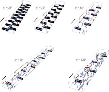
Quasi-streamwise vortices (QSVs) detected by the $\lambda _2$ technique (Jeong et al. Reference Jeong, Hussain, Schoppa and Kim1997) reach their maturity with a high population density only at LS, $s^*\geqslant 9k^*$ . In the SS cases $s^*\leqslant 3k^*$ , immature and significantly small patches of streamwise vorticity that rarely roll up into QSVs are observed in figure 14. At $s^*\geqslant 9k^*$ , on the other hand, the QSVs are well developed between the roughness elements. They reach the streamwise lengths and diameters they have in the fully developed turbulent channel flow over smooth walls when they are scaled by the local inner variables.

Figure 15.

Attached spanwise shear layers over the roughness elements $(s^*=9k^*)$ . $(a)$ The $\lambda _2^+\leqslant -0.02$ isosurfaces, and $(b)$ the spanwise vorticity, over the upstream front side. $(c)$ The $\lambda _2^+\leqslant -0.02$ isosurfaces and $(d)$ the spanwise vorticity, over the crest.

The QSVs manage the mixing process, basically between the roughness elements. Global and local heat transfer characteristics at the wall will be discussed in some detail in the next section. It seems reasonable, on an intuitive basis, to assume that the scalar transfer over the crests is mostly governed by the attached shear layers which are present in all the cases, as clearly seen in figure 14. These layers contain mostly intense spanwise vorticity $\omega _z$ , and appear essentially at the top of the roughness elements (figures 15 $c$ and 15 $d$ ). They are dominated by the $-\partial u/\partial y$ component of the spanwise vorticity $\omega _z$ . They roll-up into $\lambda _2$ structures, because they are intense on one hand and there is a natural vorticity discontinuity physically induced by the edges of roughness elements, on the other. These are some basic conditions for vorticity layer roll-ups Jiménez & Orlandi (Reference Jiménez and Orlandi1993). The spanwise rollers are coherent. They cover the entire crest in span most of the time. Their streamwise extent may reach 30 wall units, but their wall-normal thickness rarely exceeds 10 wall units, so that they are associated with flattened shear layers. The latter are occasionally lifted up to give local wall-normal vorticity, and subsequently tilt up, giving rise to patches of streamwise vorticity. This is one of the classical regeneration mechanisms provided in the vast literature on near-wall coherence (Tardu Reference Tardu2014). However, the spanwise rollers remain essentially attached structures at the crests, as revealed by a careful analysis of the movies we realised. Patches of thin spanwise vorticity layers marked by the $\partial v/\partial x$ component of $\omega _z$ , appear intermittently, at the bottom of the front $z{-}y$ sides as seen in figures 14 and 15 $(a)$ and 15 $(b)$ . They do not play an eminent role in the passive scalar transport. The shear layers identified on the $x{-}y$ lateral surfaces in figure 15(d) constitute additional topological features when contrasted with the configuration in which the roughness elements extend across the entire span ( $s^*=0$ ). These coherent vorticity layers appear to be systematically coupled with, and to coexist alongside, the spanwise rollers forming above the crests. At present, however, the causal relationship between these two structures remains indeterminate, as it is not evident whether one mechanism is responsible for regenerating the other. In this regard, the influence exerted by spanwise asymmetry on the formation of crest rollers remains an open question. Corroborative evidence from the literature, specifically concerning the absence of such structures for the case $s^*=0$ , could potentially provide clarification; nevertheless, the number of published investigations explicitly addressing this aspect is exceedingly limited. For example, a close examination of figure 17 in Nagano et al. (Reference Nagano, Hattori and Houra2004) does not yield a clear indication of spanwise rollers attached to the crests when $s^*=0$ . This observation lends credence to the hypothesis that spanwise asymmetry represents the principal mechanism underlying the phenomenon. Ultimately, however, only a rigorous analysis of the vorticity dynamics and the associated transport processes could resolve this issue definitively – an endeavour that falls outside the scope of the present study. Overall, the flow visualisations nicely show that all attached shear layers over the roughness elements are present in each $ {s^*}/{k^*} \neq 0$ configuration. They further show some key elements of the coherent structure regeneration process near the wall, such as the occurrence of hairpin vortices, which evolve into one legged structures. The reader is invited to consider the movies included as supplementary movies are available at https://doi.org/10.1017/jfm.2025.10997.

Canonical near-wall turbulence can be sustained in ‘minimal flow units’ (MFUs) of spanwise extent $l_z^+=100$ which is the streak spacing, and of streamwise extent $l_x^+=250{-}350$ that is the typical length of a single QSV (Jiménez & Moin Reference Jiménez and Moin1991). The size of the minimum flow unit is, however, too small to represent the turbulent flow field in the logarithmic and outer layers. We have already seen that there are only few QSVs regenerated between the roughness elements for small $s^*$ (figure 14) and that the flow topology at $s^*\leqslant 3k^*$ is rather governed by the structures regenerated near the roughness elements. The reason is that there is not enough space between the roughness elements to allow the QSVs to spatio-temporally develop and be sustained. The idea is to consider this region as a MFU in which the structures reach their maturity before interacting with consecutive roughness elements. This zone has therefore a streamwise extent $l^*=p^*{-}k^*$ which is the distance between two consecutive square bars, and the spanwise length $l_z^*$ of the computational domain. This is schematically shown by the red boxes in figure 14. The structures can indeed develop freely over the whole span between two consecutive staggered roughness elements provided that they have enough space in the streamwise direction, i.e. that $l_x^*$ is large enough. To further emphasise this point and to be rigorous, the scaling has to be adequate and based on the local shear velocity determined between consecutive square bars instead of $\overline {u}_\tau =\sqrt {{(H ({{\rm d}\overline {p}}/{{\rm d}x} ))}/{\rho }}$ . 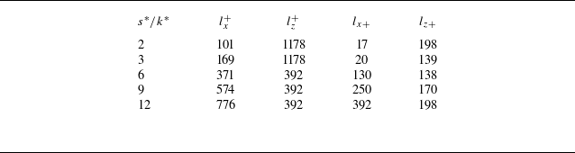The last two columns of table 2 show these length scales scaled by the local shear velocity $\overline {u}_{\tau ,l}=\sqrt { {\overline {\tau }_{w,l}}/{\rho }}$ , where the wall shear stress stands for $\overline {\tau }_{w,l}=\mu ( {\partial \langle \overline {u}\rangle }/{\partial y} )_{y=0}$ averaged over the smooth wall between the roughness elements. The spanwise extent $l_z^*=\pi$ of the computational domain was large enough to fulfil the condition $l_{z+}\geqslant 100$ for most of the cases, except for $s^*=2k^*$ and $s^*=3k^*$ . The viscous drag for these two cases is comparatively small. We performed additional (expansive) simulations for these two cases. Thus, the computational domain was increased to $l_z^*=3\pi$ by keeping the same resolution to ensure $l_{z+}\geqslant 100$ , on the one hand, and to determine the effect of the computational domain size on the results, on the other. The statistical results were closely similar for both $l_z^*=\pi$ and $l_z^*=3\pi$ . Thus, it appears that the streamwise extent of the MFU defined above is critical for the development of the QSVs. Table 2 shows that the spanwise length scaled by the local shear, $l_{z+}$ , of MFU is larger than 100 in all the cases. It is seen, however, that the flow units of the cases $s^*=2k^*$ and $s^*=3k^*$ with $l_{x+}\approx 20$ are too small to allow the coherent structures to regenerate and self-sustain in the streamwise direction.

Table 2.

Configuration of the MFUs. See the text for details.

The only cases which strictly fulfil the Jiménez & Moin (Reference Jiménez and Moin1991) conditions are $s^*=9k^*$ and $s^*=12k^*$ , and the case $s^*=6k^*$ , with the lowest bulk Reynolds number (table 1), is somewhat intermediary. This explains the lack of well-developed coherent structures between the roughness elements in the SS configurations (figure 14). The streamwise length of the QSVs scaled by the local inner variables varies roughly between 200 and 300 at $s^*\geqslant 9k^*$ as in the canonical wall turbulent flows. A multitude of snapshots in the threshold range $-0.03\leqslant \lambda _2^+\leqslant -0.01$ were inspected, leading to the same conclusions. The structures at small shifts $s^*/k^*\leqslant 3$ are triggered near and next to the roughness elements. Failing to develop in the streamwise direction, they massively agglomerate, become tangled in the spanwise direction, meander and stick between the gaps separating two adjacent staggered roughness elements. For large $s^*/k^*\gt 6$ , the spanwise communication between the staggered elements turns off, the QSVs settle down, develop and are sustained. The model we introduce here has the merit to provide satisfactory and simple explanations of the flow topology within the canopies in different configurations.

10. Global and local wall transfer characteristics

Figure 16.

$(a)$ Nusselt number for different $s^*/k^*$ cases as a function of the bulk Reynolds number $ \textit{Re}_b$ . Dotted line represents the Kays & Crawford (Reference Kays and Crawford1980) correlation, and broken line represents laminar channel flow. $(b)$ Estimated thermal efficiency under the constraints of constant pump power (circles) and constant flow rate (squares).

Here, the Nusselt number $ \textit{Nu}= {2\textit{Re}_\tau \textit{Pr}}/{\langle \overline {\theta }_b\rangle ^+}$ is expressed as a function of the hydraulic diameter $D_h=2H$ , and of the bulk temperature $\langle \overline {\theta }_b\rangle = \int _0^H\langle \overline {U}\rangle \langle \overline {\theta }\rangle {\rm d}y/\int _0^H\langle \overline {U}\rangle {\rm d}y$ . It is shown in figure 16 $(a)$ as a function of the bulk Reynolds number. Recall that $ \textit{Re}_b$ and $ \textit{Re}_\tau$ are based on the half-channel width $H$ and that the Prandtl number is $ \textit{Pr}=1$ . The Nusselt number is independent of $ \textit{Re}_b$ , as if the regime were fully rough. The dotted line in figure 16 $(a)$ shows the correlation $ \textit{Nu}=0.036\textit{Re}_b^{0.8}$ of Kays & Crawford (Reference Kays and Crawford1980) in a smooth turbulent duct flow. Recall that this relation, which is also very close to the popular Dittus–Boelter equation (Boelter et al. Reference Boelter, Cherry, Johnson and Martinelli1965), is valid for large enough Reynolds numbers $ \textit{Re}_b\gt 5\times 10^3$ . The bulk Reynolds number for the reference canonical turbulent flow at the same Kármán number $ \textit{Re}_\tau$ as in the rough channel is only $ \textit{Re}_b\approx 2\times 10^3$ here. In the absence of reliable data in the subcritical regime, we extrapolate the Kays and Crawford correlation down to $ \textit{Re}_b\approx 2\times 10^3$ . It is seen that there is an acceptable agreement between this correlation and the $ \textit{Nu}$ value we obtained in the smooth channel (closed black circle). The global wall transfer enhancement is clear in all the cases. The Nusselt number in the rough channel is four times larger than the $ \textit{Nu}=4.12$ value of the Poiseuille flow.

The thermal efficiency is the ratio $\eta = \textit{Nu}/\textit{Nu}_S$ of the actual Nusselt number to the reference case $ \textit{Nu}_S$ of a fully developed turbulent smooth channel flow. The constraint is constant pump power (Webb & Eckert Reference Webb and Eckert1972) implying that

(10.1) \begin{align} \frac {C_d(\textit{Re}_b)}{C_{\textit{ds}}(\textit{Re}_{\textit{bs}})}\left (\frac {\textit{Re}_b}{\textit{Re}_{\textit{bs}}}\right )^3=1, \end{align}

where the subindex $s$ refers to the reference smooth channel and $C_d$ is the drag coefficient. Here, $C_d=2(\textit{Re}_\tau /\textit{Re}_b)^2$ is known in the actual rough channel. Assuming a power law $C_{\textit{ds}}(\textit{Re}_{\textit{bs}}) = \textit{cRe}_{\textit{bs}}^m$ for the reference case results in

(10.2) \begin{align} \textit{Re}_{\textit{bs}}=\left (\frac {C_d(\textit{Re}_{b})}{c}\right )^{\frac {1}{m+3}}\textit{Re}_b^{\frac {3}{m+3}}. \end{align}

In order to have an estimate of the thermal efficiency, we opt for the Dean (Reference Dean1978) correlation in which $c=0.06$ and $m=-0.25$ . This leads to $ \textit{Re}_{\textit{bs}}\approx 10^3$ for the reference smooth channel, resulting again in a low Reynolds number range in which there is a general lack of reliable data both for $C_{\textit{ds}}$ and $ \textit{Nu}_S$ . Estimations of the thermal efficiency shown in figure 16 $(b)$ in which $ \textit{Nu}_S$ is further determined by the Kays & Crawford (Reference Kays and Crawford1980) correlation have therefore to be considered with care. Nevertheless, $\eta \geqslant 1$ in figure 16 $(b)$ , except for the smallest-shift case, with a maximum in the range $3\leqslant s^*/k^*\leqslant 6$ , indicating that the increase in heat transfer at the wall is at least as large as the increase in drag, under the constant pump power constraint.

The thermal efficiency under the constant flow rate constraint is $\eta _*= ( {\textit{Nu}}/{\textit{Nu}_S} )_{\textit{Re}_b}/ ( {C_d}/{C_{dS}} )_{\textit{Re}_b}$ , where the quantities are evaluated at the same bulk Reynolds number. The ratio $2\leqslant ( {\textit{Nu}}/{\textit{Nu}_S} )_{\textit{Re}_b}\leqslant 3.5$ varies relatively slowly with the geometry compared with $5\leqslant ( {C_d}/{C_{dS}} )_{\textit{Re}_b}\leqslant 14$ . The squares in figure 16 $(b)$ show $\eta _*$ versus $s^*/k^*$ . The heat transfer performance under constant flow rate is $\eta _*\lt 1$ and it is significantly low in the SS cases because of the dominance of drag $ ( {C_d}/{C_{dS}} )_{\textit{Re}_b}$ . The latter decreases with increasing $s^*/k^*$ , so that $\eta _*$ in the LS configurations becomes comparable to that reported in Nagano et al. (Reference Nagano, Hattori and Houra2004) who investigated the transverse rib-roughness morphology at larger $ \textit{Re}_b$ .

Figure 17.

$(a)$ Local temperature gradient, and $(b)$ local Kármán number, computed over the crests and at the wall between the roughness elements as a function of the bulk Reynolds number. The values between the roughness elements (broken line) and over the crests (solid line) are shown by closed and open symbols, respectively. Increasing $ \textit{Re}_b$ matches with increasing $s^*/k^*$ beginning at $s^*/k^*=3$ . The open and closed stars correspond to the case $s^*/k^*=2$ .

The local temperature gradient at the wall $ ({1}/{\Delta T}) ({\partial \langle \overline {T} \rangle }/{\partial y^*})$ is shown in figure 17 $(a)$ as a function of the bulk Reynolds number. The wall gradient is locally computed separately over the crests and between the roughness elements. It is clearly seen that $({1}/{\Delta T})({\partial \langle \overline {T} \rangle }/{\partial y^*}) $ is twice larger over the crests than in the valley, independently of $s^*/k^*$ . The wall gradient locally increases because of intense shear layers over the crests, as discussed earlier. The Kármán number $ \textit{Re}_\tau$ based on the local shear velocity determined either over the crests or between the roughness elements is additionally computed (figure 17 $b$ ). There is a satisfactory aggregation of the data, except over the crests at the smallest-shift case $s^*=2k^*$ . The corresponding plan area density in this case is $\lambda _p=0.2$ , at which the viscous drag increases following its local minimum at $\lambda _p=0.15$ , as seen in figure 3 $(b)$ . This is the consequence of the viscous shear’s dominance over the crests due to the attached spanwise rollers and the meandering of the coherent structures within the small gaps between the roughness elements (figure 4 $c$ ). It is seen that the local $ \textit{Re}_\tau$ is particularly small between the roughness elements at $s^*\lt 6k^*$ . We have shown that there is not enough space to allow the QSVs to spatio-temporarily develop between the staggered roughness elements at small $s^*/k^*$ . The wall shear stress is mainly governed by the shear stress producing eddies between the roughness elements. Since QSVs are absent or weak at small $s^*/k^*$ the turbulent wall shear they induce is low too. Thus, $ \textit{Re}_\tau$ in the valley increases almost linearly up to $s^*=9k^*$ and reaches a plateau region thereafter. In contrast, ${1}/{\Delta T}( {\partial T}/{\partial y^*})_{y^*=0}$ does not depend on $s^*/k^*$ neither at the crests nor between the roughness elements, pointing again at a local difference between the scalar and the flow fields.