1 Introduction
The International Planning Competition (IPC) is an event organized in the context of the International Conference on Planning and Scheduling (ICAPS). It has been traditionally organized biennially, even though it is recently organized every 3 years. The competition has various goals, including:
∙ providing an empirical comparison of the state of the art of planning systems;
∙ highlighting challenges the planning community has to face;
∙ proposing new directions for research and new links with other fields of artificial intelligence (AI);
∙ providing new data sets to be used by the research community as benchmarks.
Planning engines taking part in the competition are then made available (including their source code), which is very useful within and outside of the planning community. In summary, the IPC is nowadays a reference source when building technology related to AI planning, including new planning engines, planning domain model tools, problem reformulation tools, etc. The IPC also provides benchmarks in terms of problems, and evaluating metrics.
The IPC 2014 was held in three distinct parts: deterministic, learning and probabilistic. The deterministic part, which has been running since IPC 1998, is focussed on fully observable environments with instantaneous and deterministic actions. The learning part focuses on the ability of planners in learning from prior experience in order to improve their performance. The probabilistic part considers problems with stochastic transitions, and (optionally) partial observability. This paper focusses on the deterministic part, the main part of the IPC since 1998. Details and information about all the parts of IPC 2014 can be found in a survey paper (Vallati et al., Reference Vallati, Chrpa and McCluskey2015a) or on the corresponding websiteFootnote 1 .
The deterministic part of IPC 2014 followed the example given in IPC 2011 (López et al., Reference López, Celorrio and Olaya2015) in terms of continuity: IPC 2014 structure included the same tracks of IPC 2011, the same evaluation metrics and the same version of the input language. Also, along with new domains exploring new directions for planning research, domains from previous editions of IPC were used, in order to allow a good assessment of the progress in the field, and to exploit a large set of benchmark domains. Moreover, continuing the effort of previous IPC organizers in terms of transparency and reproducibility of the results, all the benchmark, source code (and description) of solvers and the huge amount of generated data have been made publicly available on the website of the deterministic part of IPC 2014Footnote 2 .
The deterministic part of IPC 2014 introduced three main innovations:
1. The agile track: this evaluated how quickly planners solve challenging problems. This has been done in order to foster the exploitation of planning-based techniques in real-time planning applications where plans are required as soon as possible.
2. A larger set of core features: to reflect the growing need to increase the expressiveness of input languages, the set of core features that participants were required to support has been extended to include negative preconditions and conditional effects. The reason behind extending the requirements was to promote the formerly neglected features that we believe are very important for real-world applications. We acknowledge that negative preconditions can be safely compiled away, as already done by some planners (see, e.g. Fast Downward and FF (Hoffmann & Nebel, Reference Hoffmann, Edelkamp, Thiébaux, Englert, dos, Liporace and Trüg2001; Helmert, Reference Helmert2006)), but having a large number of planners that can natively support such preconditions will help the knowledge engineering process in many applications. In fact, some of the introduced domains were inspired by real-world applications and require these features (see Section 3.1).
3. A protocol for problem selection: a critical step of every competition is the selection of test instances. IPC 2014 introduced a transparent and general protocol for the effective selection of testing problem instances.
The deterministic part of IPC 2014 attracted a record number of 67 submitted planners. In total, 66 researchers took part in the competition, from 15 countries: Australia, Canada, Czech Republic, Finland, France, Germany, Iran, Israel, New Zealand, Spain, Switzerland, United Kingdom, Venezuela and United States. The competition results were presented at an IPC dedicated session during ICAPS 2014. After the competition, a thorough analysis of performance and data has been performed. The overall aim of this paper is to present the results of the analysis, specifically on the following points:
∙ Structure: Section 2 describes the structure of the deterministic part of IPC 2014 in terms of rules, tracks and adopted scoring schema.
∙ Benchmarks: domains used, protocols used for selecting challenging planning tasks and the final benchmark set, are described in Section 3.
∙ Results: the main results are presented and discussed in Section 4. Section 5 analyses the complementarity of participants’ performance with regards to the considered benchmarks and metrics. The progress of the state of the art of domain-independent planning systems is assessed in Section 6.
∙ General trends: overall trends and general questions are discussed in Section 7.
2 The competition
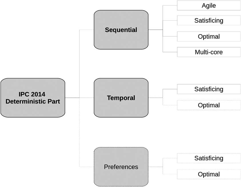
The deterministic part of the IPC was divided into three components: sequential, temporal and preferences. Although a deterministic and fully observable environment is considered for all of them, domain and problem models differ in terms of expressiveness, and the corresponding instances have different objective functions to optimize. In sequential planning, every action has an associated cost, and the metric considered is to minimize the cost of the provided plans. In temporal planning, actions have an associated duration and the objective is to minimize makespan, that is, time needed to execute the plan. Planning with preferences considers soft goals or trajectory constraints, which allow users to indicate some preferences with regards to the shape of the generated plans (Baier & McIlraith, Reference Baier and McIlraith2008). Preferences are described in terms of penalties for not achieving them, thus the quality of plans is measured in terms of net benefit, which includes penalties and the total action costs.
Each of the participating planners had to accept domain and problem descriptions in PDDL and provide output in a specified format such that plans could be validated by the VAL tool (Howey et al., Reference Howey, Long and Fox2004). There were no specific restrictions for the planners (e.g. techniques, programming languages, libraries), except that the planners were executable on the cluster used for running experiments, and supported a specified command line invocation. The number of submitted planners was restricted to two per one team in one track. This was done for avoiding an uncontrolled proliferation of very similar planning engines based, for instance, on small variations of the same planner.
Domains and problems that we used in the competition were kept secret all through the process, until the results had been announced.
2.1 Tracks
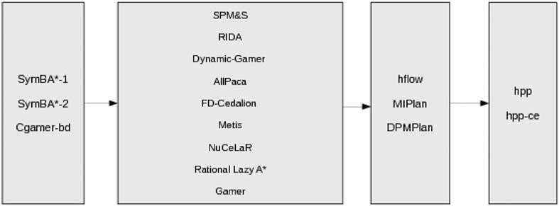
The deterministic part of the IPC 2014 had three main tracks. Figure 1 shows the overall structure of the deterministic part of competition. In the following we provide a description of each of them. For detailed descriptions of solvers, the interested reader is referred to Vallati et al. (Reference Vallati, Chrpa and Kitchin2014) or to the IPC websiteFootnote 3 .
The structure of the deterministic part of International Planning Competition (IPC) 2014. Dashes indicate tracks that have been cancelled

2.1.1 Sequential
The sequential track is the longest running track of the IPC. It focuses on classical planning, that is, the environment is static, deterministic and fully observable, and actions are instantaneous. In terms of required PDDL features (core features), apart of those that were required in the IPC 2011, we also required negative preconditions and conditional effects to be supported by participating planners. It was not mandatory for submitted planners to support all the core PDDL features; on the other hand supporting only a subset of them reduced the chances to win a track. We ran 4 sequential tracks, namely satisficing, optimal, agile and multi-core. Whereas the satisficing, optimal and multi-core tracks were present in the last competition, the agile track was new. The reason for the agile track was to re-introduce a metric for evaluating how fast we can generate plans for challenging problems. This motivates the development of ‘fast’ planning engines that can be exploited in applications.
In the sequential satisficing track, the emphasis was given to the quality of solution plans, but optimality was not required. In other words, the planners had to optimize for total action-cost of solution plans (i.e. the sum of the costs of all actions in the plan) and were given 30 minutes for each problem and 4 GB of RAM. When no action costs were explicitly provided, the total number of actions in the plans had to be minimized. Notice that the time spent for finding the best solution plan was not considered: planners were awarded the same score if they produced the same quality plans regardless of the time needed to produce them. For the satisficing track we received 43 registrations out of which 21 planners were submitted for the competition.
In the sequential optimal track, the planners had to produce optimal solution plans in the time limit of 30 minutes and 4 GB of available RAM. Planners that generated a sub-optimal solution plan for some problems were awarded 0 points for the whole domain, and disqualified if they provided sub-optimal solution plans in more than one domain. In the event, none of the competing planners had to be penalized. For the optimal track we received 34 registrations out of which 17 planners were submitted for the competition.
In the sequential agile track, the emphasis was on the speed of plan generation. In other words, the planners had to generate solution plans as quickly as possible (the time limit was 5 minutes), using at most 4 GB of RAM. In this track the quality of solution plans was not taken into account during competition scoring. For the agile track we received 21 registrations out of which 16 planners were submitted for the competition.
In the multi-core track, the emphasis was given to quality of solution plans as in the satisficing sub-track, and the time limit was also 30 minutes. In contrast to the satisficing track, four cores could be exploited, but the same overall amount of RAM (4 GB) was made available. For the multi-core track we received 17 registrations out of which nine planners were submitted for the competition.
2.1.2 Temporal
The temporal track extends the sequential track by explicitly considering time, that is, action execution is not instantaneous. The requirements of the temporal track in terms of PDDL features were the same as in the IPC 2011. In particular, neither of the extended features of negative preconditions and conditional effects was required. In the temporal track, the emphasis was to optimize makespan, that is, total plan execution time. Originally, we designed two temporal tracks: satisficing and optimal. For the temporal satisficing track we received nine registrations out of which six planners were submitted for the competition. For the temporal optimal track, only one planner has been submitted. Hence, this track was cancelled.
2.1.3 Preferences
The preferences track extends the sequential track by specifying preferences under the form of soft goals. If they are not satisfied, the total cost of the plan is increased. Similarly to the sequential track, the emphasis was given to optimize total cost of solution plans, including the ‘penalties’ for not satisfying soft goals. We had opened two preferences tracks: satisficing and optimal. However, in both tracks we received a very few submissions (2 for satisficing and 0 for optimal) and thus we decided to cancel the whole track.
2.2 Evaluation
The competing planners were evaluated using the well-known IPC score, as in recent IPCs. For each track, the planner which achieved the highest score was declared the winner. In detail, participants of the sequential satisficing and multi-core tracks were evaluated as follows. Given a planner C and a problem p,score(C,p) is defined as
 $$score\,(C,p)\,{\equals}\,\left\{ {\matrix{ 0 & {{\rm }if\,p\,{\rm is}\,{\rm unsolved}} \cr {{{N_{p}^{{\rm {\asterisk}}} } \over {N_{p} (C)}}} & {{\rm otherwise}} \cr } } \right.$$
where N
p
(C) is the cost of the solution plan of p obtained by C, and
 $N_{p}^{{\rm {\asterisk}}} $
the minimal cost of the solution plan of p among all the considered planners. The total IPC score is the sum of the scores achieved on each considered problem. The time limit was 30 central processing unit (CPU)-time minutes (wall-clock) per problem.
The solvers that took part in the sequential optimal track were evaluated as follows. For a planner C and a problem p,score(C,p) is 0 if p is unsolved, and 1 if solved (optimally). The total IPC score is the sum the scores achieved on each considered problem. The time limit was 30 CPU-time minutes per problem. Note that a planner that returned sub-optimal plans was awarded 0 points for the whole domain, or disqualified if such a behaviour occurred in more than one domain.
The sequential agile track participants were evaluated as follows. For a planner C and a problem p, score(C,p) is defined as
 $$score\,(C,p)\,{\equals}\,\left\{ {\matrix{ 0 & {{\rm }if\,p\,{\rm is}\,{\rm unsolved}} \cr {{1 \over {1{\plus}{\rm log}_{{10}} ({{T_{p} (C)} \over {T_{p}^{{\rm {\asterisk}}} }})}}} & {{\rm otherwise}} \cr } } \right.$$
where T
p
(C) is the CPU-time needed by planner C to solve problem p and
 $T_{p}^{{\rm {\asterisk}}} $
the CPU-time needed by the best considered planner, otherwise. The total IPC score is the sum the scores achieved on each considered problem. The time limit was 5 CPU-time minutes per problem. Given the large variability of runtime performance, there may be a large difference between the values of
 $T_{p}^{{\rm {\asterisk}}} $
and T
p
. The usage of an evaluation score such as the one introduced for the satisficing track would have lead to a high percentage of scores close to 0. In particular, planners with good overall coverage performance, but not excelling in minimizing runtime, would have been significantly penalized. For limiting such strong penalization, the logarithmic function has been introduced, originally in the learning part of IPC 2011.
Finally, the solvers in the temporal satisficing track were evaluated as follows. For a planner C and a problem p,score(C,p) is
 $$score\,(C,p)\,{\equals}\,\left\{ {\matrix{ 0 & {{\rm }if\,p\,{\rm is}\,{\rm unsolved}} \cr {{{M_{p}^{{\rm {\asterisk}}} } \over {M_{p} (C)}}} & {{\rm otherwise}} \cr } } \right.$$
where M
p
(C) is the makespan of the solution plan of p, obtained by C and
 $M_{p}^{{\rm {\asterisk}}} $
the minimal makespan of the solution plan of p among all the considered planners, otherwise. The total IPC score is the sum the scores achieved on each considered problem. The time limit was 30 CPU-time minutes per problem.
2.3 The development environment system
With an increasing number of complex and sophisticated competing planners, the traditional way of submitting planners (via e-mail) becomes extremely time consuming on the organizers. Typically, issues might arise with different configurations of the hardware, of the operating system, different versions of libraries, etc. Therefore, in case of any complication, the organizers must, first, identify the exact issue and then have to communicate with the authors of the planner, in order to fix any problems with the running of the planner. However, giving the authors the ability to compile and test their planners directly on the machine used for the competition, eliminates this significant overhead. Moreover, the competitors are able to form a view of the performance of their system on the competition premises, as different hardware or software configurations can affect the performance of solvers (Howe & Dahlman, Reference Howe and Dahlman2002).
Hence, we introduced the development environment system (DES) system for the submission and on-site testing phase of the planners. Several months before the submission deadline of the planning software, each team was granted Secure SHell access to a node of the actual competition cluster. More than 10 GB of space for user data was made available to each team, which had a private directory assigned. In each private directory we put a set of example instances—also provided via the IPC website—including a number of problems from several domains with different PDDL features requirements.
Authors were able to compile and test their system on the provided set of simple example instances, or on other instances that they uploaded to the cluster. For running tests, 1 GB of RAM and 1 CPU was available for each team, and a maximum of 64 simultaneous accesses was allowed to the DES system.
In the case of specific requirements, such as installing required packages or libraries, the authors exploited a ticketing system. Tickets were handled by cluster administrators and recorded for security purposes.
The DES system was also exploited for submitting planners. By the submission deadline, the authors were required to upload to their home directory the source code—following a naming convention described on the competition website and circulated using the competition mailing list—and a PDDL support questionnaire.
2.4 Bug fixing
By using the DES system, authors were able on their own to identify bugs and issues in their planners that were related to the hardware and software configuration of our cluster. This was evidenced by e-mail exchanges with authors and DES system administrators. Although it was the authors’ responsibility to submit bug-free planners, we allowed bug fixing after the planners’ submission deadline after a request from the authors or when we identified some issues with the planners. Hence authors were allowed to fix bugs, but not to update other parts of the code. For this reason, patches were analyzed in order to avoid major changes. In the case where we identified that a planner behaves oddly, that is, no or very few problems solved in several domains—with a focus on newly introduced domains—we investigated the planner’s logs in order to identify the source of such odd behaviour. If the evidence of potential bugs was found, we tried to replicate it on different instances: small problems from domains not considered in the benchmark set. In the end, logs and small problems were then sent to teams, who were given 1 week for fixing the bugs and providing a patch. This happened for three teams.
3 Benchmarks
The process used in the selection of benchmark domains, benchmark domain models and subsequently benchmark problem instances within those domains, is of central importance to the competition. Given a domain and its requirements, there are many domain models that can be chosen to represent it, and for each model, there are many choices of problem instances. The selection process is an important issue for the whole research area, as competition benchmarks are used for evaluating and assessing subsequent works in planning. Substantial work has been done by organizers of previous editions of the IPC for identifying ‘good’ benchmarks (Hoffmann et al., Reference Hoffmann and Nebel2006). Our guide was to make choices in line with the reasoning behind past IPCs, and hence we constructed a set of explicit requirements as follows. The set of IPC benchmarks should:
∙ be externally interesting: they should support the potential exploitation of automated planning in real-world scenarios;
∙ be interesting in relation to representation: collectively they should test the full range of the core PDDL features;
∙ preserve competition continuity: a significant proportion of the benchmarks used should be extracted from past competitions;
∙ be encoded with only the declared core PDDL features: every submitted planner should be capable of attempting to solve the planning problems;
Further, problem instances of each domain model must be selected:
∙ to be challenging and discriminating: selected instances must be hard to solve, at least for proven state-of-the-art planning systems, within the time allotted; and they must provide a way to rank the planners (rather than, e.g. being too easy or too hard for all of them);
∙ to be without any bias (apart from the point above): the instances must be generated by a process without hidden bias, except to make the set challenging and discriminating.
From the start of the competition till the revealing of the results, all the choices made were kept secret from the competitors.
3.1 Selection of domains and domain models
A total of 23 different domain models were used in IPC 2014, each encoding a different domain. To retain continuity, 14 were reused from previous IPCs, and nine domains were new. Also, following the reasoned decision taken by the IPC 2011 organizers, a single PDDL model per domain was used (López et al., Reference López, Celorrio and Olaya2015). Among the new domains, five were designed by the organizers:
∙ CITYCAR: this domain aims to simulate the impact of road building/demolition on traffic flows. A city is represented as a directed graph, in which each node is a junction and edges are ‘potential’ roads. Cars start from their initial positions and have to reach their final destination as soon as possible. There is a finite number of roads available, which can be built for connecting two junctions and allowing a car to move between them. Roads can also be removed, and placed somewhere else, if needed. In order to place roads or to move cars, the destination junction must be clear, that is, no cars should be in there.
∙ HIKING: this domain has been designed for planning a long—multiple days—hike for small groups of people. A planner has to deal with decisions such as transporting tents, where to park cars for later use, etc.
∙ MAPANALYSER: this is a temporal version of the citycar domain, extended by considering that vehicles can have different speed, and that the time needed for building or removing roads depend on their length.
∙ RTAM: this domain deals with a situation which arises immediately after a traffic accident has been reported. This involves police for securing the area, fire brigades for extinguishing fire or freeing trapped victims, paramedics and ambulances for providing first aid and transporting accident victims to hospitals, and tow trucks for removing damaged vehicles from the accident scene.
∙ TETRIS: this is a simplified version of the well-known Tetris game. All the pieces are randomly distributed on a N×N grid. The goal is to move them in order to free the upper half of the grid. The pieces can be rotated or translated. Each movement action has a different cost, according to the size of the piece.
Four domains were collected via the call for domains:
∙ CAVEDIVING: a number of divers has to explore an underwater cave, by taking pictures of some specified areas of the cave. There are a set of available divers, each of who can carry four tanks of air that are needed for exploring the cave. These divers must be hired before going to the cave and either take photos or prepare the way for other divers by dropping full tanks of air. Certain divers have no confidence in other divers and will refuse to work if someone they have no confidence in has already been in the cave. Divers have hiring costs inversely proportional to how hard they are to work with.
∙ CHILDSNACK: this domain is focussed on the problem of making and serving sandwiches to a group of children, in which some are allergic to gluten. The available ingredients have to be combined in order to prepare the required number of sandwiches.
∙ GED: the problem is to find a min-cost sequence of operations that transforms one genome (signed permutation of genes) into another. The purpose of this is to use this cost as a measure of the distance between the two genomes, which is used to construct hypotheses about the evolutionary relationship between the organisms.
∙ MAINTENANCE: this is a simplified planning/scheduling problem. There are mechanics/equipment who on any day may work at one of several airports (hubs) where the maintenance facilities are present, in order to check or repair airplanes. The airplanes are visiting some of the airports on given days. The problem is to schedule the presence of the mechanics/equipment so that each plane will get maintenance once during the required time period.
Five additional domains were submitted by researchers in response to the call for domains, but were not included in the competition. Some of them required non-core PDDL features that only few planners supported and thus were not consistent with our requirements; while with others it was not possible to identify a suitable set of benchmark problem instances, due to low randomization of generators or the high complexity of even small instances for state-of-the-art planners.
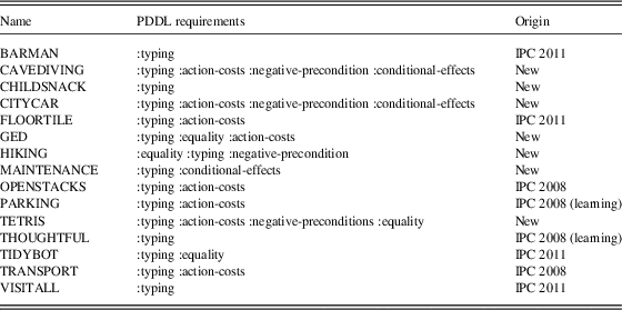
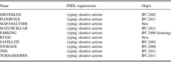
Tables 1 and 2 show the list of domain models used in the sequential and temporal tracks, respectively. As an exception, tidybot was used in the sequential optimal track only; it substituted thoughtful, which was used in other tracks. This was due to the fact that no generator is provided for the thoughtful domain, and the instances used in the learning track of IPC 2008 were too complex for the submitted optimal planners. thoughtful was intentionally selected for the other tracks, however, because its large number of operators makes it a particularly challenging domain model for planners.
Domains used in the sequential satisficing, sequential optimal, sequential agile and multi-core tracks of International Planning Competition (IPC) 2014

It should be noted that TIDYBOT has been used in sequential optimal track only; in other tracks it has been substituted by THOUGHTFUL.
Domains used in the temporal satisficing track of International Planning Competition (IPC) 2014

Some of the newly introduced domains were selected due to the fact that they test planners’ ability in solving problems which involve different, and possibly large, sets of PDDL requirements. This is the case of CAVEDIVING, HIKING, MAINTENANCE and TETRIS, that require negative precondition and/or conditional effects. Furthermore, a few domains deal with (simplified) real-world problems, that can represent a potential future application of planning techniques. This is the case for domains dealing with different aspects of traffic controlFootnote 4 , such as RTAM, CITYCAR and MAPANALYSER, and the problem of finding a minimum cost sequence of operations for transforming one genome into another (Haslum, Reference Haslum2011), encoded in the GED domain. The childsnack domain is interesting in that it requires planners to take into account limited resources.
In all the domain models that include conditional effects, that is, CAVEDIVING, CITYCAR, and MAINTENANCE, there is one operator of the model that has one conditional effect. It is worth mentioning that in the maintenance domain model there is only one operator, and its only effect is a conditional effect. This makes the MAINTENANCE domain model of particular interest for assessing the ability of planners in dealing with conditional effects.
After the competition, it was reported by participants that some planner parsers may have faced issues in a few of the benchmark domain models, which included domain models used in previous editions of the IPC. These issues are as follows:
∙ In THOUGHTFUL, a domain model introduced in IPC 2008, a predicate and a type have the same name. Remarkably, this is not forbidden by the PDDL specification, and it is accepted by PDDL-related tools, such as the VAL validator (Howey et al., Reference Howey, Long and Fox2004).
∙ In CAVEDIVING and MAINTENANCE, conditional effects were not explicitly listed in the PDDL features requirements, though the: adl requirement, which encompasses conditional effects, was listed.
∙ Action costs requirements were not listed in GED and FLOORTILE domain models.
∙ The RTAM domain model had one dummy operator, not needed for solving planning instances, which requires a not defined predicate.
Updated versions of the benchmarks have been made available on the IPC website. Discussion about the potential impact of the described PDDL issues on the results is left to Section 4.
3.2 Selection of problem instances
Once we selected a domain and encoded a representation of the domain’s actions within a model, the difficult problem of producing a set of benchmark problem instances has to be solved. As in IPC 2011, we decided to select 20 problems per domain, requiring 460 problems in total.
We required a systematic, transparent and general method, that is one which others can follow in order to produce the same (sort of) problems, and can apply to any set of planners, on any domain. Also, the method must produce instances satisfying the overall requirements in terms of producing benchmark problem instances which are challenging and discriminating for the considered set of solvers that have to be compared. Hence the instances generated must not result in all problems being solved trivially, or all unsolvable, by each competitor.
In some areas of Artificial Intelligence, the complexity of problems can be evaluated statically, before the use of solvers, by considering the phase transition (Kanefsky & Taylor, Reference Kanefsky and Taylor1991; Rossi et al., Reference Rossi, Van Beek and Walsh2006). This is not generally the case in planning, where phase transition has been demonstrated only for randomly generated graphs (Bylander, Reference Bylander1996; Rintanen, Reference Rintanen2004) but where the features that make an instance hard to solve are unknown. Moreover, in automated planning complexity is also related to the domain model used, and the space of instances that can be generated is constrained by available random generators. Remarkably, some work has been done in automated planning for assessing, to some extent, the complexity of planning instances. The recently introduced Torchlight tool (Hoffmann, Reference Hoffmann2011) provides a route to analyze search space topology under the delete-relaxation heuristic. On the other hand, it does not provide information about the performance of planners based on different approaches. Therefore, the only viable way for selecting benchmark problem instances based on how difficult they are, is dynamically—in other words trying to solve them with a planner. Assuming that in general, the performance of competition planners has improved over current state of the art planners, in IPC 2014 we used a protocol for selecting, within a given domain, a suitable set of instances by utilizing the competition planners, as follows:
For each target domain:
1. identify size, in terms of number of objects involved;
2. given the sizes, generate between 30 and 50 instances per domain, using available random generators;
3. anonymize planners;
4. run all the planners on the generated instances;
5. collect results, in terms of solved problems and quality of solutions;
6. order problems by number of planners which solved them;
7. select 20 benchmarks.
In the first step, if the domain was used already in previous IPCs, then the sizes of larger benchmark problems (top half) are taken, and possibly extended following the ‘trend’ used by organizers. The size of a benchmark is given by the number of objects involved. Specifically, if random generators are available, the value of required input parameters describe the size. Since different sizes are usually considered within a set of benchmark instances, the sequence of increasing number of different objects give us the trend. Otherwise, some well-known planners, namely LPG (Gerevini et al., Reference Gerevini, Saetti and Serina2003), Metric-FF (Hoffmann, Reference Hoffmann2003), LAMA-11 (Richter & Westphal, Reference Richter and Westphal2010), probe-11 (Lipovetzky & Geffner, Reference Lipovetzky and Geffner2011), Madagascar-11 (Rintanen, Reference Rintanen2012) and SGPlan5 (Chen et al., Reference Chen, Wah and Hsu2006), are used for identifying a reasonable size range. These planners have been selected due to their good performance in previous IPCs, and to the fact that they exploit very different planning approaches, hence limiting the bias towards a specific approach. However, given the small number of parameters that is usually made available by random planning problem generators, and the diversity of the planning approaches exploited by participants, it is not always possible to generate and select—even with a good selection protocol—a suitable benchmark set. If no random generator is available, all the available instances have been considered.
In step 7, 20 instances are selected according to the observed coverage performance, so that they show the following properties:
∙ Interestingness: no more than the 80% of the anonymized solvers are able to solve all the 20 instances;
∙ Solvability: no more than the 80% of the anonymized solvers are unable to solve any instance;
∙ Short-lead: the delta of solved instances between first and second solvers, according to coverage, is less than 50%.
The rationale behind the first and second properties is very intuitive, that is, avoid too trivial and too complex instances. The third property aims at avoiding the selection of benchmarks in which only a single planner excels.
The most complex set of instances that satisfies the mentioned properties, is selected. Here complexity is measured in terms of coverage. Ties are broken by considering the length of the best plan for each problem: the problem with the highest cost is identified as the most complex. If there is no set of 20 benchmarks that satisfies all the three properties above, then the process is started again from step 1, by considering different sizes.
The described protocol was used for selecting benchmarks for the sequential satisficing and temporal satisficing tracks. Exactly the same instances were used in the sequential agile track.
Benchmarks for the other tracks were then derived from such sets as follows. Slightly smaller benchmarks have been selected (following steps 3–7) for the sequential optimal track, and some slightly larger instances have been selected for two domains (BARMAN and THOUGHTFUL) of the multi-core track. This was done because optimal planning is harder than satisficing in practice (Helmert, Reference Helmert2003; Helmert & Röger, Reference Helmert and Röger2008), and because parallel planners can exploit more resources than purely sequential solvers. Some overlaps are present in the different sets.
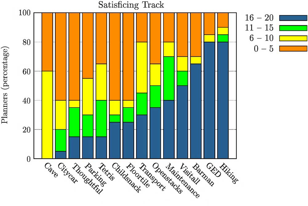
Figure 2 shows for each domain the percentage of planners, from the sequential satisficing track, able to solve different number of problems. We focus on four classes, with a step of five instances. In a nutshell, this gives an overview of planners with a large coverage (16–20 instances solved), planners struggling to solve instances from the considered domain (0–5), and planners that solve a bit more (11–15) or a bit less (6–10) than 50% of the instances. In most of the domains, at least 40% of the solvers are able to solve a large number of instances. This does not apply to cavediving, in which at most seven instances are solved by 60% of the solvers, and citycar, where a single planner is able to solve more than 15 instances, but the 20% of the competitors are able to solve between 11 and 15 instances. All in all, Figure 2 confirms that selected instances are not favouring a single planner, because a large number of instances is usually solved by a significant percentage of solvers. At the same time, the fact that not all the planners are able to solve all the instances from a domain, and that the set of planners solving all the instances varies among domains, indicate that the benchmarks are useful for comparing and discriminating planners’ performance.
For each domain, the percentages of sequential satisficing planners able to solve: more than 16 instances (blue); between 11 and 15 instances (green); between 6 and 10 instances (yellow); and between 0 and 5 instances (orange).

From a general point of view, the proposed protocol introduces a potentially strong bias towards the participating planners. This is because, out of the initial large set of instances, the actual benchmarks are selected by considering the performance of the participants. Even though this reduces the generality of the benchmarks, that is, solvers that are based on very different approaches than those used by participants can show unpredictable performance, the focus on participants guarantees that benchmarks can provide useful information for ranking submitted solvers, which is one of the aims of the competition. Moreover, given the range of approaches exploited by submitted solvers, and given the number of existing planners considered in step 1, we are confident that benchmarks are also of interest for planners that did not take part in the IPC. Also, in other prominent AI competitions, such as the SATisfiability (SAT) competition, similar selection protocols for benchmarks have been used since 2012 (Balint et al., Reference Balint, Belov, Diepold, Gerber, Järvisalo and Sinz2012, Reference Balint, Belov, Heule and Järvisalo2013; Belov et al., Reference Belov, Diepold, Heule and Järvisalo2014; Vallati & Vaquero, Reference Vallati, Chrpa, Grzes, McCluskey, Roberts and Sanner2015).
Specifically, in SAT competitions benchmarks for application and hard combinatorial tracks are selected as follows. First, the empirical hardness of SAT instances is evaluated by using five well-performing solvers, taken from the previous edition of the competition. Instances are then divided into four classes, according to the average runtime and to the solvability: easy, medium, hard and too hard. Easy instances, corresponding to instances solved by all the considered solvers in less than 1/10th of the competition’s timeout—are removed because they are believed to be uninformative. Then the selection process is guided by considering a few constraints, aiming at maximizing the number of new instances—that is, not used in previous competitions—and keeping a 50-50 ratio between medium and hard instances. Evidently, the described protocol suffers from potentially strong biases towards the solvers used for classifying instances.
Finally, in recent Answer-Set Programming competitions a protocol very similar to the described above—strongly based on the observed performance of existing solvers—is used (Calimeri et al., Reference Calimeri, Gebser, Maratea and Ricca2016).
3.3 Empirical complexity of selected benchmarks
In order to evaluate the empirical complexity of benchmarks used in the deterministic part of IPC 2014, we performed a domain by domain analysis. We carried out an investigation for each track both from the problems’ and from the planners’ perspective. The former is represented as the fraction of problems solved by all the participants for the given domain, and it was calculated as follows:
 $${\rm Solved}\,{\rm Problems}\,{\equals}\,\left( {\mathop{\sum}\nolimits_{n{\equals}1}^P {} {{C_{n} } \over {P{\rm {\asterisk}}N}}} \right){\times}100$$
, where P is the number of planners, N the number of problems of the domains and C
n
the number of problems of the considered domain solved by the nth planner.
A value of 100 indicates that all the planners solved all the instances of the given domain; on the contrary, a value of 0 indicates that no planner solved any instance. Similarly, the planners perspective is represented as the fraction of planners that solved all the problems of the domain.
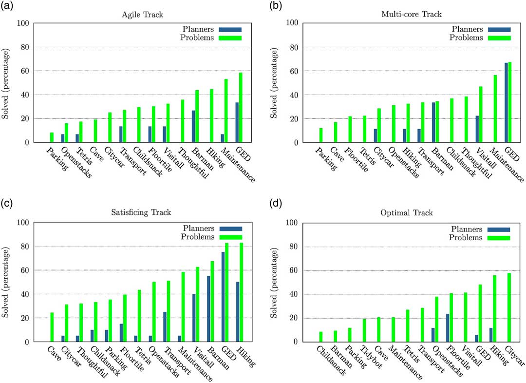
Figure 3 shows the results of the domain by domain analysis on (a) sequential agile, (b) multi-core, (c) sequential satisficing and (d) sequential optimal tracks. Domains are ordered according to the percentage of solved problems. Given the results shown, it is possible to derive that: (i) the PDDL requirements do not strongly affect the complexity of selected benchmarks. Domain models with various requirements are spread among the graphs; (ii) multi-core planners are not as mature as sequential planners. Considering that benchmarks are the same for all domains but two, results clearly indicates that multi-core planners are less performant; and (iii) few problems are solved in the optimal track. We noticed that selecting problems for the optimal track is very challenging, mainly because performance of solvers do not scale smoothly; therefore planners tend to be very fast or to not solve at all.
Fractions (in percentage) of problems solved by all the participants (green) and fractions of planners that solved all the problems (blue) of a specific domain in the (a) sequential agile, (b) multi-core, (c) sequential satisficing and (d) sequential optimal tracks

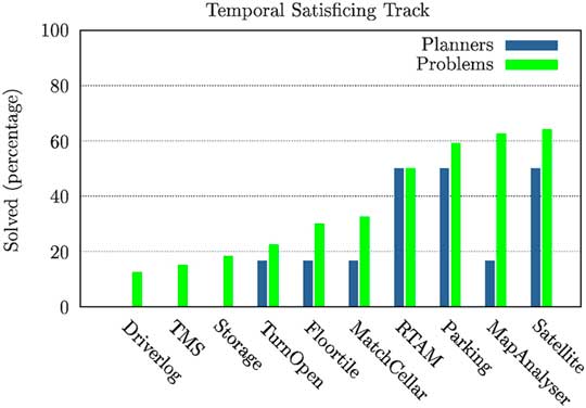
Figure 4 shows the results of the domain by domain analysis on the temporal satisficing track; also in this case, domains are ordered according to the percentage of solved problems. Most of the instances selected for the newly introduced MAPANALYSER and RTAM domains are solved by the participants, even though—especially in MAPANALYSER—only a few planners are able to solve all the benchmarks. Remarkably, as observed also in IPC 2011, concurrency makes planning tasks hard to solve: this is the case of instances from MATCHCELLAR, TMS and TURNANDOPEN domains. On the other hand, the complexity of DRIVERLOG and STORAGE instances is due to their size: in order to make them challenging, a large number of objects are involved.
Percentages of problems solved by all the participants (green) and percentages of planners that solved all the problems (blue) of a specific domain in the temporal satisficing track

With regards to the previously given intuition of good benchmarks, we observed that in sequential agile and temporal satisficing tracks benchmarks are generally informative. In sequential satisficing, it can be noticed that benchmarks of some domains look too easy. Multi-core and satisficing optimal benchmarks were challenging for the participants.
4 The results of the competition
This section is devoted to comparing planners’ performance and to identify those that won awards. Our underlying assumption is that planning problems are considered as solved by a given planner if it returns a valid plan, and unsolved otherwise. Validity of plans was assessed using VAL (Howey et al., Reference Howey, Long and Fox2004). Given that, our analysis is focused on three features:
∙ the quality of provided solutions using metrics based on solution size;
∙ the coverage of planners using metrics based on number of solved instances;
∙ the efficiency of planners using metrics based on runtime.
In order to provide an improved view of the performance of participants, as well as presenting the results using the IPC score, we present how planners would have been ranked according to the Borda count. In addition, we use statistical analyses to place planners into groups depending on whether their ranking is statistically significant. Furthermore, we provide a summary level discussion of the potential impact of PDDL issues (presented in Section 3.1) on the results.
The Borda Count is a single-winner method used in elections and in other AI competitions (e.g. International Competition on Computational Models of ArgumentationFootnote 5 (Thimm et al., Reference Thimm, Villata, Cerutti, Oren, Strass and Vallati2016)). We used it in the following way. Given a track, for each domain participants are ranked according to the evaluated metric (i.e. IPC score or coverage). Given n participants, the first planners for the specific domain get n points, the second n−1, the third n−2, etc. The Borda count of a planner in a track is the sum of the points that planner got among the considered domains. Intuitively, the Borda count ranks planners according to their ‘general’ performance on the full set of considered domains. The performance of participants in terms of quality and runtime was compared using a statistical analysis based on the Wilcoxon sign-rank test (Wilcoxon & Wilcox, Reference Wilcoxon and Wilcox1964) and the Binomial test. These tests have been applied to a set of paired observations and allow us to decide if it is possible to assume that there is no correlation between the pairwise observed quantities. In order to deal with the well-known issue related to the use of multiple pairwise tests, namely the increased risk of type I error, the Bonferroni correction has been exploited. However, it should be noted that the use of such correction may lead to an increased number of type II errors—that is, observations are believed not be statistically different, while they are. For the sake of our analysis, given the fact that statistical tests are used among other approaches for comparing planners’ performance, the potential presence of type II errors is not critical, as planners can be compared using the other provided metrics.
The Binomial test has been used for comparing the number of solved instances of planners participating in a track. This is an exact two-tailed test that measures if the provided distributions—in terms of successes—are statistically different. Data points are pairs of 0 and 1: ‘1’ for instances solved by the considered planner, and 0 otherwise. The null hypothesis is that the two planners perform similarly, and it is accepted for p-value>0.05; otherwise the hypothesis that the solvers perform differently is accepted for the given confidence level.
The Wilcoxon sign-rank test is used for comparing performance in terms of either quality or runtime of two participants in a track on the instances of the corresponding track. When considering the quality of solution plans, for instance, ‘no correlation’ between the observed quantities indicates that it is equally like that one solver provides a better quality problem than the second solver, than the vice versa. For the purposes of this analysis, the Wilcoxon sign-rank test is appropriate because it does not require any knowledge about the sample distribution, and makes no assumption about the distribution.
Given a sufficiently large number of samples, the T-distribution used by the Wilcoxon sign-rank test is an approximation of a normal distribution, which is characterized by the z-value and the p-value. The higher the z-value, the more significant the difference of the performance of the compared solvers is. The p-value indicates the required level of significance of the performance gap. In our analysis we considered that the null hypothesis, that is, the performance of compared solvers is statistically similar, is accepted when p-value>0.05. Otherwise, the null hypothesis is rejected, and therefore the compared solvers performance is statistically different.
Since the Wilcoxon sign-rank test compares sets of paired observations, it is of critical importance to deal with cases in which one observation has an unknown value. This happens when considering unsolved instances. For dealing with unknown entry values, we reviewed approaches exploited in previous IPCs (specifically third, fifth and seventh) (Long & Fox, Reference Long and Fox2003; Gerevini et al., Reference Gerevini, Haslum, Long, Saetti and Dimopoulos2009; López et al., Reference López, Celorrio and Olaya2015) and decided to handle such cases by mainly following the method used by the organizers of IPC 2011. When comparing plans quality we considered only double hits, that is, pairwise entries in which both values are known; this is done for reducing the impact of covering, otherwise dramatically favouring participants that solve a large number of instances. When analyzing runtime (agile track only) we assigned twice the cutoff time (600 seconds) to cases that were not solved. On the contrary, in previous IPCs the cutoff time was assigned to unsolved instances. In the agile track, given the short amount of time available for solving benchmarks, assigning exactly the cutoff time is penalizing solvers that provided solutions with runtimes close to the maximum allotted CPU-time. Therefore, we preferred to emphasize the difference between solved and unsolved instances, by considering 600 seconds for unsolved ones. If the actual cutoff time is used, we observed that the performance of many planners tend to be indistinguishable, thus the informativeness of the statistical analysis is reduced.
The results of the statistical tests are used to generate a directed graph per track of the deterministic part of IPC 2014. The nodes of the graph are the participants, and an edge from a node N 1 to a node N 2 indicates that N 1 performed statistically better than N 2. Similar graphs have been used for presenting the results of previous IPCs (Long & Fox, Reference Long and Fox2003; López et al., Reference López, Celorrio and Olaya2015) and also for configuring portfolio-based planning approaches (Gerevini et al., Reference Gerevini, Saetti and Vallati2014). For the sake of readability, planners are grouped. Members of the same group have no statistically significant difference in their performance. Considering two groups G i and G j , with G i → G j : the fact that a planner p 1 is a member of group G j indicates that at least one planner from G i is statistically better than p 1. Specifically, this indicates that all the planners in a group G n represent the pareto frontier, considering the evaluated metric, with regards to following groups.
It should be noted that the results of the statistical analysis shown in this section cannot necessarily be easily generalized. They refer to the considered planners solving the selected benchmarks, run on the specific hardware and software configuration used during the competition. It is well-known that: (i) hardware and software differently affect solvers (Howe & Dahlman, Reference Howe and Dahlman2002); (ii) the exploitation of different benchmarks can lead to different results (Howe & Dahlman, Reference Howe and Dahlman2002); (iii) running more than once randomized solvers can show different runtime distribution (Hurley & O’Sullivan, Reference Hurley and O'Sullivan2015); and finally, even considering the same benchmarks, (iv) different configurations of the domain and problem models can affect the overall results (Howe & Dahlman, Reference Howe and Dahlman2002; Vallati et al., Reference Vallati and Vaquero2015c).
4.1 Performance of sequential satisficing track participants
The sequential satisficing track is the track with the largest number of participants. In the following the results of this track are analyzed from different perspectives.
4.1.1 Number of problems solved
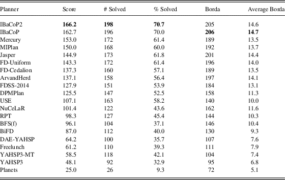
Table 3 shows the results of the sequential satisficing track in terms of IPC score, number of solved problems, success rate and Borda score for all the entrants. It is evident that the two versions of IBaCoP ranked first both in terms of coverage and IPC score. Remarkably, IBaCoP and IBaCoP2 are the only systems that were able to solve problems in all the considered domains. These planners are portfolio-based, and exploit a sequential portfolio of a large number of ‘basic’ solvers for solving a given planning task. IBaCoP solves each instance by using a fixed 12-planner portfolio, configured according to planners’ performance on some training data. IBaCoP2 instead selects, for solving each instance, the five planners that—accordingly to its predictive models—have the highest chances to solve the considered instance.
International Planning Competition (IPC) score, number of problems solved, success rate, Borda score and average Borda score for the sequential satisficing track participants

Bold indicates best result, according to the corresponding metrics. Solvers are ordered following IPC score.
Interestingly, only a few planners would have been ranked differently by using the number of solved problems as metric.
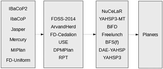
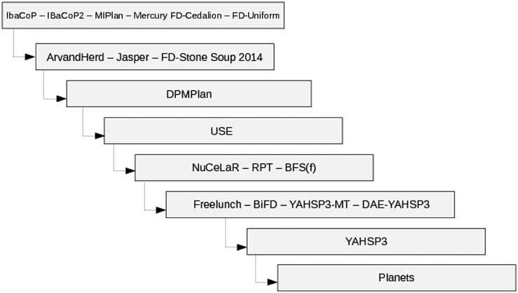
Figure 5 shows the partial order of participants according to the statistical test on coverage. Most of the participants are distributed in three large groups. This is possibly due to the fact that many engines were able to solve very similar sets of planning tasks. The first group include planners solving between 192 and 168 instances (70.7–60.0%). Then planners solving between 163 and 127 instances (58.2–45.4%) have been grouped together. The third group includes planners able to solve between 122 and 92 planning tasks. The last group is composed by Planets, only. This solver was able to successfully handle 9.3% of the considered benchmarks.
Partial order for planners in the sequential satisficing track in terms of coverage

4.1.2 Quality of plans
According to results shown in Table 3, the best performing planner in terms of quality of solutions found is IBaCoP2, that obtained 3.5 points more than IBaCoP. The third system according to IPC score is then Mercury, with an overall score of 153.0 points. It can be noted that in the top half of the table there are no large IPC score differences between differently ranked participants; this is not true for the second half, where large differences can be observed between the performance of DPMPlan and USE, BiFD and DAE-YAHSP and, finally, YAHSP3 and Planets.
It is worth noting that Planets obtained the best ratio between coverage and IPC score (0.96). Such good ratio indicates that almost every time Planets solved a problem, it found the best quality plan. It solved problems from five domains and most of the instances (14) have been solved in THOUGHTFUL.
Evaluating the performance of planners in terms of Borda score leads to ranks similar to those achieved by considering IPC score. Generally, this indicates that performances are evenly spread across the competition domains. The only exception is ArvandHerd, that according to Borda would have been ranked fourth. This planner obtained the best IPC score in four domains, and the second best in two.
Figure 6 shows the partial order of sequential satisficing entrants according to the Wilcoxon signed-rank test, on plan quality, with a p-value of 0.05. Differently from Figure 5, in this case solvers are spread across a large number of groups. The largest group includes six planning engines, while the average size is approximately two. This suggests that the performance of planners tend to be statistically different and there is a high complementarity between the planners.
Partial order for planners in the sequential satisficing track in terms of plan quality according to the Wilcoxon signed-rank test using double hits only

4.1.3 Potential impact of reported PDDL Issues
To the best of our knowledge, PDDL issues described in Section 3.1 in the Maintenance, CAVEDIVING, GED and FLOORTILE domains did not significantly affect any of the participants. With regards to the PDDL issue in the THOUGHTFUL domain, this affected all the planners of the track that exploit the Fast Downward PDDL parser, namely, all the competitors except for DAE-YAHSP, BFS(f), Planets, YAHSP3-MT and YAHSP3. However, planners were affected differently. Portfolio-based planners, such as IBaCoP and MIPlan, were affected, but were still able to solve a large number of instances by running non-Fast Downward-based solvers. Hence, portfolio-based planners that include solvers which are not based on the Fast Downward framework are not expected to obtain a significant performance improvement. For this reason, it is hard to assess how the picture changes when using a modified PDDL domain model, supported by the Fast Downward translator.
Recall that 20.0 IPC score points can be gained—in the satisficing track—by a planner that is able to provide the best solution on all the 20 benchmarks of a single domain. Among the participants that were able to solve problems from the THOUGHTFUL domain, achieved IPC scores are between 17.1 and 5.0. If the competition was rerun, Mercury, the top-ranked planner which did not solve any problems in the THOUGHTFUL domain, would need to score more than 9.7 points to obtain second position, and would need to score more than 13.2 points to achieve best position. In both cases, however, this assumes that the scores of IBaCoP and IBaCoP2 would not also improve. Picking out other planners affected, Freelunch, given the small gap from DAE-YAHSP, could gain one position; Jasper and FD-Uniform could overcome MIPlan.
4.1.4 Distinguished performers
According to results, in terms of IPC score, shown in Table 3, the following planners were distinguished by their performance in the sequential satisficing track of IPC 2014:
∙ Winner: instead of nominating two variants of the same planner as winners, the one that achieved the best IPC score was chosen as winner. The planner selected was IBaCoP2, which scored 166.2 points in total.
∙ Runner-up: Mercury was chosen as runner-up.
The declared winner, IBaCoP2, is a portfolio-based planner, a different type of planner to the winner of IPC 2011. Since 2011 portfolio-based planners have undergone significant research and development resulting in new planning features being proposed (see, e.g. Cenamor et al., Reference Cenamor, De La Rosa and Fernández2012; Fawcett et al., Reference Fawcett, Vallati, Hutter, Hoffmann, Hoos and Leyton-Brown2014), and different techniques for combining planners into a portfolio being developed (Vallati et al., Reference Vallati, Hutter, Chrpa and McCluskey2015b). As a result of the work done in the area, portfolio-based solvers are more reliable and effective, in that they can better predict the performance of basic components in order to combine them effectively. Also, most of the portfolios that took part in IPC 2011 were using different heuristics, within the same planning framework, as basic components. This was not the case in IPC 2014, where portfolios are exploiting very different solvers, with a clear benefit in terms of robustness: using different frameworks limits the potential impact of bugs or inefficiencies of the code.
The above discussion and the observed results lend much weight to the hypothesis: for satisficing planning, when a large amount of CPU-time is given, it is possible to effectively combine different planners.
4.2 Performance of sequential agile track participants
The agile track was firstly introduced in the IPC in 2014, in order to evaluate how quickly planners solve challenging problems and foster the development of fast solvers. In many planning applications it might not be possible to wait a long time until a plan is available; satisficing plans are required as soon as possible in order to provide a first response. Plans can possibly be optimized in a second step.
4.2.1 Number of problems solved
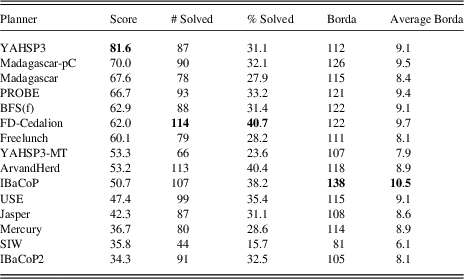
Table 4 shows the results of agile track in terms of IPC time score, number of solved problems, success rate and Borda score for all the entrants.
International Planning Competition (IPC) time score, number of problems solved, success rate, Borda score and average Borda score for the agile track participants

Bold indicates best result, according to the corresponding metrics. Solvers are ordered following IPC score.
In terms of coverage, FD-Cedalion and ArvandHerd are the planners that solved the largest number of planning tasks, respectively 114 (40.7%) and 113 (40.4%). Differently from the other tracks of IPC 2014, no entrant solved very few benchmarks. SIW, the system that solved the smallest number of problems, showed a coverage of 15.7%.
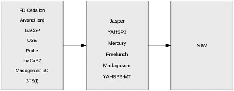
Figure 7 shows results for the statistical test on coverage. It is easy to identify three sets of similarly performing planning engines. Remarkably, first and second groups include most of the participants. This is because the number and the set of solved problems are very similar between them. The third group includes SIW only, that solved less than 24% of the considered benchmarks.
Partial order for planners in the agile track in terms of coverage

4.2.2 Analysis of central processing unit-time
The results shown in Table 4 clearly indicate that the ‘fastest’ solver (according to IPC time score) is YAHSP3, that obtained 81.6 points. A large number of planners obtained a score in the ranges 70.0–60.0 and 53.3–47.4. Remarkably, YAHSP3 is also the solver with the highest coefficient of ratio between the number of problems solved and the IPC time score (0.94). This means that when YAHSP3 solved a planning task, it was usually the fastest solver. However, it is worth noting that about 60 points out of 81.6 were obtained in three domains only: GED, TRANSPORT and VISITALL. In other words, YAHSP3 obtained the best IPC time score because it excelled in a very small set of benchmarks. This behaviour is also emphasized by the very different rankings that the three metrics shown in Table 4 (IPC time score, coverage and Borda score) lead to. FD-Cedalion and ArvandHerd provided the best coverage, but tend to be slow. In the case of FD-Cedalion, this is possibly due to a known aspect of static sequential portfolios configuration: it is generally ‘easy’ to select an effective set of solvers, but ordering the selected engines for minimizing runtime is extremely hard. The version of ArvandHerd that took part in the agile track runs a random walk-based planner for the first 3 minutes, and then uses LAMA as a backup solver. In several cases, planning tasks have been solved by the LAMA system. Despite their impressive performance in the sequential satisficing track, in the agile track IBaCoP and IBaCoP2 suffered from issues similar to those faced by FD-Cedalion. In IBaCoP, a fixed sequential portfolio—exploiting short runs of different solvers—is used: as already mentioned, this approach leads to good coverage results, but does not really optimize runtime. IBaCoP2 instead selects five solvers using its learnt predictive model and order them according to the confidence. Each solver is then allocated 60 CPU-time seconds. According to the observed results, IBaCoP2 ordering strategy is not able to effectively identify the most promising solver to be run first. Moreover, the chosen portfolio members could not solve the problems in less than 60 seconds each.
The Borda score provides a different perspective on results, and highlights the generally good performance of IBaCoP. Even though IBaCoP did not excel neither in terms of runtime nor coverage, it obtained the highest Borda score. A domain by domain analysis revealed that regardless of runtime, its good coverage allows IBaCoP to achieve an average rank of fifth on considered domains.
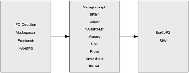
Figure 8 shows the partial order of agile entrants according to the Wilcoxon signed-rank test, on runtime. It is worth reminding that in this analysis unsolved planning instances have been assigned the double of the cutoff CPU-time (i.e. 600 CPU-time seconds). Remarkably, a large group of similarly performing solvers have been identified. The first group includes Madagascar, FD-Cedalion, Freelunch and YAHSP3. This is possibly because such solvers provide either a good trade-off between runtime and coverage, or are able to quickly solve a number of instances. The largest group is the second, which includes almost all the remaining planners. The last group includes SIW and IBaCoP2: the first has been penalized because of the small number of solved problems. IBaCoP2 is the solver with the smallest ratio between IPC time score and coverage.
Partial order for planners in the agile track in terms of runtime according to the Wilcoxon signed-rank test. For this analysis, unsolved planning instances have been assigned the double of the cutoff central processing unit (CPU)-time (i.e. 600 CPU-time seconds)

4.2.3 Potential impact of reported PDDL issues
PDDL issues reported for the Maintenance, CAVEDIVING, GED and FLOORTILE domains did not affect any of the participants. With regards to THOUGHTFUL domain, the reported issue affected all the planners which exploit the Fast Downward PDDL parser, namely: ArvandHerd, FD-Cedalion, Freelunch, IBaCoP2, IBaCoP, Jasper, Mercury and USE. From the IPC results perspective, the situation differs from the sequential satisficing track: the winner of this track was almost 20 points ahead of the nearest affected planner (Freelunch). Additionally, the THOUGHTFUL domain model results in a huge number of grounded actions which the Fast Downward PDDL parser, with its reliance on I/O operations, is sensitive to.
4.2.4 Distinguished performers
According to the results, in terms of IPC score, shown in Table 4, the following planners were distinguished by their performance in the sequential agile track of IPC 2014:
∙ Winner: YAHSP3, with an overall score of 81.6 and 87 problems solved.
∙ Runner-up: Madagascar-pC was chosen as runner-up, with a final score of 70.0 and 90 problems solved.
4.3 Performance of multi-core track participants
The multi-core track was introduced in IPC 2011 to foster the development and to evaluate the performance of this planning trend. Rules of this track have been described in Section 2.1.
4.3.1 Number of problems solved
Table 5 shows the results of multi-core track in terms of IPC score, number of solved problems, success rate and Borda score for all the entrants.
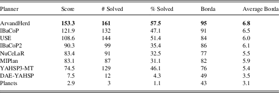
International Planning Competition (IPC) score, number of problems solved, success rate, Borda score and average Borda score for the multi-core track participants

Bold indicates best result, according to the corresponding metrics. Solvers are ordered following IPC score.
In terms of coverage, ArvandHerd solved the largest number of problems (161) and outperformed the second best planner in terms of coverage, USE (144 solved problems) by 17 planning tasks. A domain by domain analysis indicates that the better coverage of ArvandHerd mainly comes from two domains: CITYCAR and TETRIS.
Two planners, namely DAE-YAHSP and Planets, solved a small number of planning tasks. Interestingly, these two solvers took also part in the sequential satisficing track, but in that case they solved a larger number of problems. It should be noted that benchmarks between sequential and multi-core tracks are different in two domains only: BARMAN and THOUGHTFUL. Even if we ignore such domains, performance of the sequential versions are significantly better than multi-core performance. Interestingly, also IBaCoP and IBaCoP2 planners solved a larger number of planning instances in the satisficing track. Evidence suggests this can be due to the different scheduling strategies. IBaCoP systems exploit a sequential portfolio while in the multi-core track, they run concurrently one basic solver on each available CPU. Since the available amount of RAM is limited to 4 GB for both tracks, this means that less memory is available for the basic solvers in the multi-core track, leading to a large number of cases in which the portfolios run out of memory.
It is also noticeable that YAHSP3-MT solved a large number of problems: it would have been ranked 4th according to coverage. On the other hand, the quality of provided solutions is usually quite low.
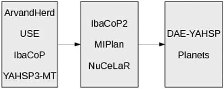
Figure 9 shows results for the statistical test on coverage. Planners have been divided in three groups of similarly performing solvers. Unsurprisingly, ArvandHerd, USE, IBaCoP and YAHSP3-MT are in the first group. This is due to the fact that these planners solve a large number of benchmark instances. The second group includes solvers that successfully handled between 99 and 87 tasks. Finally, DAE-YAHSP and Planets are in the last group.
Partial order for planners in the multi-core track in terms of coverage

4.3.2 Quality of plans
According to the results shown in Table 5, the best performing planner in terms of quality of solutions found is ArvandHerd, which obtained 153.3 points. Such remarkable results is probably due to the fact that ArvandHerd exploits both anytime search on each core, exploiting both LAMA (Richter & Westphal, Reference Richter and Westphal2010) and specifically configured random walks algorithms, and post-processing optimization: every solution found is analyzed using the Aras system (Nakhost & Müller, Reference Nakhost and Müller2010) in order to be improved. ArvandHerd is the best one also according to the Borda score. This indicates that it was usually able to achieve good performance on all the benchmark domains. Generally, the Borda score (as well as the average Borda score) leads to a ranking that is very similar to the ranking resulting by considering the IPC score. Intuitively, it is reasonable to conclude that multi-core participants performance are homogeneous among the considered domains.
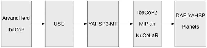
Figure 10 shows the partial order of multi-core entrants according to the Wilcoxon signed-rank test, on plan quality, considering only double hits—that is, instances solved by both compared planners. As it is apparent, partial orders in Figures 10 and 9 are very different. In terms of plan quality, five groups have been identified. ArvandHerd and IBaCOP are in the first group, and many of the solvers have been moved to the fourth group. USE and YAHSP3-MT, which were indistinguishable in terms of coverage, show statistically different performance according to plan quality.
Partial order for planners in the multi-core track in terms of plan quality according to the Wilcoxon signed-rank test using double hits only

It should be noted that statistical comparisons involving Planets and DAE-YAHSP lead to very small sample sizes. It is well-known that in such cases, the rank test may not have sufficient information to detect a significant difference between the performances. Even though this was not observed in most of the comparisons of our analysis, this could explain the reason why Planets and DAE-YAHSP have been included in the same group.
4.3.3 Potential impact of reported PDDL issues
To the best of our knowledge, PDDL issues reported for the Maintenance, CAVEDIVING, GED and FLOORTILE domains did not affect any of the participants. With regards to the PDDL issue in the THOUGHTFUL domain, this affected all the planners of the track that exploit the Fast Downward PDDL parser, namely: ArvandHerd, IBaCoP, IBaCoP2, MIPlan, NuCeLaR and USE. This means that all the top six planners, according to official results, have been affected. Evidence suggests that significant result changes are hard to imagine. Portfolio-based planners, such as IBaCoP systems, MIPlan and NuCeLaR were still able to solve a number of instances by running non-Fast Downward-based solvers: therefore no significant improvements are expected for this type of planners. The gap between ArvandHerd and IBaCoP is expected to furtherly increase, assuming that ArvandHerd system solves a few instances. Finally, based on the assumption that out of 20.0 IPC points that can be gained from the instances of a single domain, around 10.0 can be gained by solvers based on the Fast Downward framework, the rank of USE would not change, given the 13.3 IPC points gap from IBaCoP.
4.3.4 Distinguished performers
According to the results, in terms of IPC score, shown in Table 5, the following planners were distinguished by their performance in the multi-core track of IPC 2014:
∙ Winner: ArvandHerd, with an overall score of 153.3 and 161 problems solved.
∙ Runner-up: IBaCoP was chosen as runner-up, with a final score of 121.9 and 132 problems solved.
4.4 Performance of sequential optimal track participants
As in IPC 2011, no optimal domain specific planners were developed for any of the benchmarks. Therefore, it is not guaranteed that the solutions provided were always optimal. However, we believe it is safe to assume that if all the planners—or at least those able to solve it—found a solution of the same cost for a given planning task, this solution can be reasonably considered as the optimal one. Additionally, we found no evidence to suggest that any of the planners returned non-optimal solutions.
4.4.1 Number of problems solved
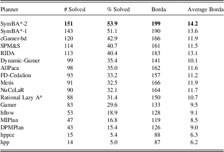
Table 6 shows the results in terms of number of solved problems (coverage) and Borda score for the sequential optimal track participants. We do not show the IPC score. This is because we checked that all the solutions were of the same quality: therefore, the score assigned to each planner for a given planning task can be either 1 (optimally solved) or 0 (unsolved). This exactly corresponds to the number of solved problems. No planner generated invalid solutions.
Number of problems solved (optimally), success rate, Borda score and average Borda score for the sequential optimal track participants

Bold indicates best result, according to the corresponding metrics. Solvers are ordered following coverage.
In terms of Borda score, planners ranking is quite similar to ranking obtained by considering the number of solved problems, in most of the cases minor changes—1 or 2 ranks—can be observed. This indicates that planners solved problems from all the considered domains. The most remarkable differences are Metis and NuCeLaR, that would have been fourth and fifth, respectively, following the Borda score. This indicates that these two planners perform generally good in all the considered domains: the average Borda scores show they are usually ranked as sixth on the considered domains. On the other hand, they do not excel in any of them.
Figure 11 shows results for the statistical test on coverage. It is easy to identify four different groups of solvers. The first group includes the two top-ranked systems, that solved 151 and 143 instances, and cGamer-bd. The second group includes solvers that optimally solved between 114 (SPM&S) and 83 (Gamer) planning tasks. The third group considers systems solving between 53 (hflow) and 43 (DPMPlan) instances. The last group comprises the two versions of hpp solving, respectively, 15 and 14 instances. We also notice that there is a large overlap when comparing the number of problems simultaneously solved by planners in the first group. For instance, cGamer-bd solved only seven problems that SymBA*-2 was not able to solve. This is not always the case for pairs of planners from the second or third group.
Partial order for planners in the sequential optimal track in terms of coverage

4.4.2 Potential impact of reported PDDL issues
To the best of our knowledge, empirical evidence suggest that the PDDL issues reported for the Maintenance, GED and FLOORTILE domains did not significantly affect any of the participants. It has been reported that RIDA solver requires conditional effect to be explicitly listed in the PDDL feature list of the domain model: for this reason, RIDA performance on instances from the CAVEDIVING domain could be affected. Given the fact that no participating solver has been able to solve more than seven instances in that domain, we can safely estimate the maximum impact as a +4 on the number of solved instances, which would allow RIDA to gain one position in the table.
It has also been reported that in barman, Maintenance and tetris, the problem generators provided, respectively, 6, 15 and 3 unsolvable tasks. Given the limited coverage shown by participants, it is not believed that this issue, in the Barman and Tetris domains, had any significant impact on the rankings. In contrast, most of the participants solved almost all the (solvable) Maintenance instances. Exceptions are cGamer-bd and gamer, which did not solve any instance; therefore, in the presence of a larger number of solvable instances from this domain, these two planners would have been penalized, with regards to the current competition outcome.
4.4.3 Distinguished performers
According to results, in terms of number of solved instances, shown in Table 6, and to the statistical analysis performed, the following planners were distinguished by their performance in the sequential optimal track of IPC 2014:
∙ Winner: instead of nominating two variants of the same planner as winners, the one that solved the larger number of problems was chosen as winner. The planner selected was SymBA*-2, which solved 151 problems in total.
∙ Runner-up: cGamer-bd was chosen as runner-up, given the number of problems solved, 120 in total.
In contrast to the results of IPC 2011, no portfolio-based solvers gained awards. Evidence points to there being a set of reasons for this break in trend. First, it has been empirically shown that algorithm selection and combination approaches for optimal planning do not generalize well on previously unseen domains (Rizzini et al., Reference Rizzini, Fawcett, Vallati, Gerevini and Hoos2015). Second, all the portfolio approaches that took part in the optimal track of IPC 2014 exploited a very similar set of basic solvers, which is a subset of the participants of IPC 2011. Third, binary decision diagrams-based solvers significantly improved their performance since IPC 2011 (Edelkamp et al., Reference Edelkamp, Kissmann and Torralba2015), mainly because of advancements in techniques which are responsible of the computation of successors and in approaches for pruning the search space (Torralba & Alcázar, Reference Torralba and Alcázar2013; Torralba et al., Reference Torralba, Edelkamp and Kissmann2013). Fourth, most of the top performing planners of IPC 2014 exploited some form of bidirectional search, which has recently achieved remarkable results in many domains.
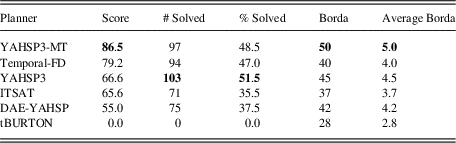
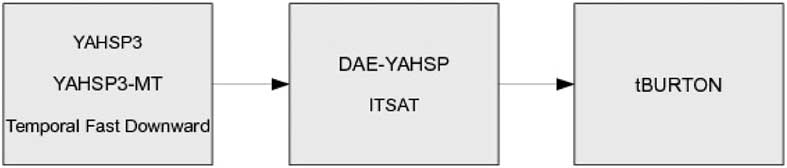
4.5 Performance of temporal satisficing track participants
This subsection is devoted to the analysis of performance of entrants in the temporal satisficing track. In this track, planners are required to solve planning tasks that involve durative actions which can temporarily overlap and/or interfere. Also, quality of plans is not measured in terms of plan cost, as in other tracks, but in terms of makespan. In fact, no cost has been defined for any action, but the duration of actions represent their ‘cost’, for the competition purposes.
As already discussed, concurrency is a critical aspect of temporal planning, and is generally hard to handle by existing planning approaches. Moreover, the presence of concurrency does not allow a planner to find sequential plans by ignoring temporal constraints, but it requires to explicitly consider temporal relations between actions. In IPC 2014, three domains (taken from IPC 2011) required concurrency: MATCHCELLAR, TMS and TURNANDOPEN. In all three domains, the plans found by DAE-YAHSP, YAHSP3 and YAHSP3-MT were invalid, according to validator VAL, because of missing information about the time-epsilons. It was not possible to clearly identify the time-espilons, despite several manual tests. Such invalid plans are not considered in the rest of this subsection.
4.5.1 Number of problems solved
Table 7 shows the results of the temporal satisficing track in terms of IPC score, number of solved problems, success rate and Borda score for all the entrants.
International Planning Competition (IPC) score, number of problems solved, success rate, Borda score and average Borda score for the temporal satisficing track participants

Bold indicates best result, according to the corresponding metrics. Solvers are ordered following IPC score.
One planner did not solve a single problem: tBurton. The reason of such behaviour is unclear, it can either be due to not very optimized code or to poor algorithm design, since the planner was able to solve very small instances—which were used for checking the presence of bugs—only.
According to the Binomial test, which results are shown in Figure 12, three groups of similarly performing planners can be identified. In the first group, planners solving from 103 to 94 instances are included. The second group includes solvers that solved between 71 and 75 instances. The last group includes tBurton, only.
Partial order for planners in the temporal satisficing track in terms of coverage

4.5.2 Quality of plans
According to the results shown in Table 7, the best performing planner is YAHSP3-MT, with an IPC score of 86.5 Interestingly, this planner did not solve any instance that required concurrency, but performed extremely well on the remaining planning tasks. This justifies the high IPC score. The high Borda score is due to the fact that three participants were not able to provide valid solutions to problems from the domains that require concurrency, that the number of participants is small, and that tBURTON did not solve any of the problems. Therefore, even if no problem from MATCHCELLAR, TMS and TURNANDOPEN has been solved, the Borda score is still very high, as well as the average Borda score. It is worth noting that the highest coefficient of ratio between the number of problems solved and the IPC score was achieved by ITSAT (0.92). On the other hand, this is mainly due to the results obtained in three domains: FLOORTILE (18.8 score), MATCHCELLAR (19.0 score) and TMS (18.0 score).
Figure 13 shows the partial order of temporal satisficing entrants according to the Wilcoxon signed-rank test, on plan quality, with a p-value of 0.05. The reported analysis considered only double hits, therefore tBURTON could not be ranked. Temporal-FD and YAHSP3-MT do not show statistically different performance, but they are statistically better than YAHSP3. Finally, ITSAT and DAE-YAHSP are included in the final group. The fact that ITSAT is in the third group, even though it showed the best ratio between solved problems and IPC score is mainly due to the use of double hits: many of the problems solved by ITSAT are not solved by other participants.
Partial order for planners in the temporal satisficing track in terms of plan quality according to the Wilcoxon signed-rank test using double hits only. It should be noted that tBURTON cannot be related to any other planner due to the fact that it did not solve any planning task

4.5.3 Potential impact of reported PDDL issues
According to the results of the competition, Temporal-FD did not solve any instance from the RTAM domain. This seems to be due to the PDDL issue described in Section 3.1. When using the updated domain model, Temporal-FD can handle instances from this domain; however, plans provided by YAHSP3-MT tend to be of better quality, thus we do not expect any significant change in ranks of the competition.
The other reported issues did not affect the performance of any of the competitors.
4.5.4 Distinguished performers
According to the results, in terms of IPC score, shown in Table 7, the following planners were distinguished by their performance in the temporal satisficing track of IPC 2014:
∙ Winner: YAHSP3-MT is the planner that obtained the best IPC score, 86.5.
∙ Runner-up: Temporal-FD was chosen as runner-up.
4.6 Most innovative planning systems
With the aim of fostering the development of new and innovative planning approaches, IPC 2014 introduced the most innovative planning systems award. In contrast to the newcomer award of IPC 2002 (Long & Fox, Reference Long and Fox2003), the focus of the award for the most innovative planning system is on promoting new ideas, rather than acknowledging the difficulty of building new planning systems. In fact, because of the number of planning frameworks available, the deployment of a new planner is nowadays a task that does not require a large team of programmers and developers.
For selecting the most innovative planning systems, the organizers took into account: (i) the novelty of the exploited planning techniques—qualitatively assessed by considering planner descriptions—and (ii) the overall performance. Two planners were jointly given the award: Mercury and RPT. The former is based on the red-black heuristic, which relaxes only some state variables in order to achieve a balance between taking advantage of delete-relaxation and mitigating its drawbacks (Domshlak et al., Reference Domshlak, Hoffmann and Katz2015). RPT exploits rapidly exploring random trees in order to decompose planning tasks into much smaller subtasks that connect randomly generated (non-spurious) states (Alcázar et al., Reference Alcázar, Veloso and Borrajo2011).
5 Complementarity of planners
In this section, we evaluate the complementarity of planners that took part in the tracks of IPC 2014. Specifically, we are interested in investigating if different solvers provide good performance (according to the considered metrics) on different sets of planning tasks, thus can be combined in order to improve overall performance. A related concern is to investigate if a set of planning engines outperforms the winner of each track. We should be careful, however, in generalizing these results as they refer to the competition planners and benchmarks: using different benchmarks may lead to significantly different complementarity results.
The data used in this analysis were obtained as follows. Given a track of the deterministic part of IPC 2014, we considered all the possible portfolios P
i
of, respectively, 2, 3 and 4 component planners
 $c_{j}^{i} $
. Each component
 $c_{j}^{i} $
is a planner j that took part in the analyzed track. For each planning instance, the performance of a portfolio P
i
corresponds to the performance of the best component
 $c_{b}^{i} $
. In other words, we show the performance of the Virtual Best Solver: an Oracle that, given a planning problem and a set of between 2 and 4 planning engines, is always able to select the best solver according to the considered metric. The number of generated portfolios ranges between 510 (temporal track) and 123 500 (sequential satisficing track).
The outlined approach allows us to assess the usefulness of combining different planning techniques, regardless of training issues. Specifically, it provides the best result achievable by combining different planners. It should be noted that here we are interested in evaluating the best possible complementarity of planning engines rather than in understanding the capabilities of portfolio approaches in combining IPC 2014 participants or learning from IPC 2014 benchmarks. In terms of learning approaches, the learning track of IPC 2014 compared the state of the art of learning for planning. For information about portfolio approaches in planning, the interested reader is referred to Núñez et al. (Reference Núñez, Borrajo and López2015), Rizzini et al. (Reference Rizzini, Fawcett, Vallati, Gerevini and Hoos2015), Vallati et al. (Reference Vallati, Hutter, Chrpa and McCluskey2015b); a thorough discussion about mining IPC 2011 results can be found in Cenamor et al. (Reference Cenamor, De La Rosa and Fernández2012).
Table 8 shows the results of the performed analysis in terms of selected planners, IPC score and coverage of portfolios of different sizes, on the tracks of IPC 2014. For the sake of readability, and for assessing the maximum achievable performance, only results of the best portfolios are shown. Portfolios (in terms of both components and planner selected for solving a specific planning instance) can be different according to the optimized metric. We do not report IPC score results of portfolios on the optimal track, since in that track only coverage is considered.
Size, selected solvers (alphabetically ordered), International Planning Competition (IPC) score and percentage of solved problems achieved by portfolios including from two to four components, and the best single solver

According to results shown in Table 8, it is possible to effectively combine planners that took part in the sequential agile track. Remarkably, the set of benchmarks where YAHSP3, Madagascar and Freelunch achieve good performance are almost disjoint. This is because, by combining them using the Oracle portfolio, the IPC score achieved is very similar to the sum of the IPC scores of each single planner (see Table 4). Interestingly, adding a fourth system (PROBE) can still improve the overall performance in terms of IPC score, but not as much as in the previous cases. IPC score is also improved when considering the ‘worst’ possible portfolios, that is, the combination of planners achieving the lowest IPC score, ranging between 50.7 points (2 planners) to 66.2 (4 planners). The presence of complementary planning engines in the sequential agile track is confirmed also in terms of coverage.
Results obtained in multi-core, sequential satisficing and temporal satisficing tracks in terms of IPC score are similar to the results shown for the agile track. Also in these tracks combining more planners lead to better IPC scores. On the other hand, while the improvement obtained by considering two planners instead of one is usually significant, adding more planners leads to small improvements. Beside the complementarity of planners, this difference is also possibly emphasized by a number of circumstances: (i) sequential agile track participants generally solved less problems than other tracks participants, and (ii) runtime performance can vary much (orders of magnitude), while quality of plans tends to be more similar between solved instances. Also, in the case of coverage, the outlined behaviour is confirmed: a large improvement is obtained by considering two-planner portfolios. When considering larger sets of planners, improvements are less significant.
Table 8 also shows that planners that took part in the Optimal track show a low level of complementarity. The largest improvement is obtained by considering two planners instead of one: this results in 17 (6.1%) more planning instances being solved. In the other tracks of IPC 2014, the smallest improvement, in terms of coverage, obtained by considering two-planner portfolios instead of a single solver has been achieved in the sequential satisficing track, where 51 (18.2%) more planning instances can be solved. To some extent, the low complementarity of optimal track participants can also be due to the selected benchmarks: according to the results shown in Section 3.3, benchmarks used in the optimal track are extremely challenging.
6 Comparisons between 2014 planners and older planners
In this section we compare the performance of the winners of IPC 2014 with previous IPC winners. This can provide evidence about the progress of the state of the art of domain-independent planning engines, though there are various factors and biases that have to be taken into account:
1. IPC benchmarks are used extensively for testing planners and for tuning purposes. The default values of planners’ parameters are set—either manually or automatically—by evaluating the impact of the possible values on the available benchmarks; such benchmarks largely come from previous editions of the IPC. Similarly, portfolios are combined according to the performance of planning engines on those benchmarks. This is common practice in the planning community, and providing challenging benchmarks is one of the contributions of the IPC. However, it is likely that IPC 2014 competitors have been tested and ‘tuned’ on benchmarks from previous IPCs. Further, while planners in previous competitions were tuned this way, the latest batch of planners would have access to a greater range of benchmarks than previous planners. Therefore, IPC 2014 planners tested on benchmarks from previous competitions may provide a flawed or biased progress evaluation.
2. The generation of benchmarks for IPC 2014 involved the competition planners themselves, to ensure that problem instances were challenging (but not too much). In part, the generation also involved past winners of competitions in the first step of benchmark generation. These factors can be seen as a bias towards the planners (or the set of planners) involved, as the benchmarks were chosen dependent on the results.
Given these factors, we decided to compare past IPC winning planners (in particular from IPC 2011) with IPC 2014 benchmarks, and if improved versions of past winners were available, these were used in this analysis. This in the spirit of providing a fair comparison: it is well-known that competition submissions are usually the result of very deadline-oriented development, which can possibly lead to bugs or poorly engineered code. Also, where possible, we compared the performance of planners that took part in both 2011 and 2014 planning competitions, with the aim of providing more reliable evidence of progress.
6.1 Sequential agile track
The agile track in its current form has been introduced in IPC 2014, therefore there are no winners of previous editions to compare with. In order to investigate the progress of the state of the art in terms of runtime, we decided to consider three domain-independent planners that are commonly seen as ‘fast’ satisficing solvers: FF (Hoffmann & Nebel, Reference Hoffmann, Edelkamp, Thiébaux, Englert, dos, Liporace and Trüg2001), LPG (Gerevini et al., Reference Gerevini, Saetti and Serina2003) and the latest available version of the well-known LAMA (Richter et al., Reference Richter, Westphal and Helmert2011) solver, which was stopped after it found the first solution. They were executed on the same hardware and software configuration used for running the IPC 2014. As with the competition planners, these planners may be subject to some bias as they (or versions of them) were involved in benchmark selection.
The results were that LAMA would have been ranked 11th, LPG would have been ranked 13th, and FF would have been ranked 17th out of 17 participants. LAMA solved a large number of instances, 97 (34.6%), but obtained an IPC score of 48.2. The other two planners solved many fewer instances, but were generally faster: LPG solved 54 (19.3%) instances and obtained an IPC score of 39.6; FF solved 28 (10%) planning tasks and obtained an IPC score of 21.9. The Wilcoxon test confirmed the statistically significant difference between LAMA, LPG and FF performance and the winner of the IPC 2014 agile track, YAHSP3.
In IPC 2014 a number of core PDDL features have been introduced and are used in a few domain models (see Table 1). In particular, conditional effects are not supported by LPG. For this reason we decided to remove domain models exploiting such features (namely, mapanalyser, maintenance and cavediving) from the comparison. In that case, LPG would have been ranked 9th, between Madagascar and USE. Also in this case, however, the performance of YAHSP3 are statistically better than the performance of LPG.
The results of the performed analysis are twofold. On the one hand, there is a significant difference in runtime performance between previous fast solvers and the winners of the 2014 Agile competition using the 2014 benchmarks. However, this improvement in runtime has not been driven by recent IPCs, which focused on quality of plans. On the other hand, both LPG and FF were released more than a decade ago, and they did not have the benefit of being tuned on recent benchmarks, yet their performances are still comparable with those of the IPC 2014 participants. This indicates that, although there is a recognizable progress, it could have been more marked.
6.2 Multi-core track
The multi-core track was first introduced in IPC 2011 (López et al., Reference López, Celorrio and Olaya2015). As observed in 2011, the participation is usually much lower than in the traditional sequential tracks. This was confirmed also in 2014.
The winner of the multi-core track in 2011 was ArvandHerd (Valenzano et al., Reference Valenzano, Nakhost, Müller, Schaeffer and Sturtevant2012) (hereinafter, ArvandHerd11). A significantly improved version of ArvandHerd (hereinafter ArvandHerd14) is also the winner of the 2014 edition. In order to assess the improvement of the state of the art, we ran ArvarndHerd11—in which a few bugs have been fixed by the authors—on the IPC 2014 benchmarks, and compared its performance against the current winner. The results indicate that ArvandHerd11 is able to solve 136 instances (47.6%) against 161 (57.5%) of ArvandHerd14. In terms of the IPC score, ArvandHerd11 obtained 134 points, while ArvandHerd14 obtained 154.7. Performances are similar in terms of the number of best solutions found: 109 versus 104 for the 2014 version. The most prominent difference was noticed in the GED domain, where the 2011 version of ArvandHerd was not able to solve any instance, while ArvandHerd14 solved all of them. According to the authors, this is very likely due to the exploitation of a newly developed translator—used for encoding PDDL problems into SAS+—by ArvandHerd14. Most of the difference between the two planning engines derives from the performance gap in the GED domain. The results therefore suggest that there is not a significant improvement in the state of the art of multi-core planning, at least with regard to the IPC 2014 benchmarks.
In order to compare the performance of state-of-the-art multi-core and sequential planning systems, we ran the winner of sequential satisficing track, namely IBaCoP2, on the multi-core benchmarks. IBaCoP2 has been run on a single core, according to the rules of the sequential track. Benchmarks between these two tracks are different in two domains only, barman and thoughtful. Results indicate that on the multi-core benchmarks, IBaCoP2 shows a better coverage than ArvandHerd14: they solved 179 and 161 problems, respectively. Moreover, IBaCoP2 is usually able to provide better quality plans, as indicated by the better IPC score: 167.0 and 155.6 for IBaCoP2 and ArvandHerd14, respectively. Finally, by simulating a new competition which includes all the multi-core systems and the winner of the sequential satisficing track, we observed that IBaCoP2 would have been able to win such a competition. Interestingly, a multi-core version of IBaCoP2 took part in the 2014 multi-core track, but it performed poorly: we believe this is due to design/engineering issues and, as discussed in previous sections, also to the fact that IBaCoP system runs four different planners concurrently, thus reducing the available amount of RAM for each solver. It should be noted that the analysis was performed using the same time bounds. However, for the multi-core track 30 minutes is the wall-clock time—this basically means that a multi-core planner can exploit 2 hours of CPU-time—while the sequential satisficing planner got 30 minutes CPU-time. From the outlined results, it is still appears to be the case that—as it was in 2011—multi-core planners perform worse than single-core satisficing planners.
6.3 Sequential optimal track
The winner of the sequential optimal track in IPC 2011 was FDSS-1 (Helmert et al., Reference Helmert, Röger and Karpas2011). Since it was not entered in IPC 2014, a refined version of FDSS-1 was used for performance comparison. Given the fact that FDSS-1 is built on top of the Fast Downward framework, we considered the latest available version of the framework, and ran the planner using the FDSS-1 configurationFootnote 6 . In this way, FDSS-1 is also able to handle the PDDL core features that have been introduced in IPC 2014.
According to the analysis performed, the optimal planner that won IPC 2014 shows significantly better performance than FDSS-1 in terms of coverage on the IPC 2014 testing instances. SymBA*-2 solved 53.9% of the IPC 2014 benchmarks, while FDSS-1 was able to solve 36.8%: FDSS-1 solved 48 less instances than SymBA*-2. The difference in performance is statistically significant also according to the Binomial test. On the other hand, FDSS-1 solved 18 planning tasks that were not solved by SymBA*-2.
In the IPC 2014 competition, FDSS-1 would have been ranked sixth out of 18 participants. In three of the considered domains, FDSS-1 was able to solve as many problems as the best solver: MAINTENANCE, PARKING and CAVEDIVING. In two domains, namely BARMAN and CHILDSNACK, the planner did not solve any problems due to the complexity of the problem instancesFootnote 7 .
In order to provide a better overview of the progress of the state of the art of optimal planning between IPC 2011 and IPC 2014, we also evaluate the performance of Merge-and-Shrink (Nissim et al., Reference Nissim, Hoffmann and Helmert2011), LM-cut (Helmert & Domshlak, Reference Helmert and Domshlak2011) and the 2011 version of gamer, hereinafter gamer11. Merge-and-Shrink and LM-cut show very good performance in the 2011 optimal track; they were ranked fourth and fifth, respectively. They are both built on top of Fast Downward framework. Therefore, as previously done for the evaluation of FDSS-1, the latest available version of the framework has been used. In our experimental analysis, Merge-and-Shrink solved 29.6% of the IPC 2014 benchmarks, and LM-cut was able to solve the 26.8%. They would have both been ranked 14th out of 18 participants (17 IPC 2014 participants plus the considered solver). They did not solve any instance from the BARMAN, CHILDSNACK and CITYCAR domains, due to the hardness of the benchmark set.
A version of the gamer planner also took part in the sequential optimal track of IPC 2014: we will refer to such version as gamer14. gamer11 was able to solve the 18.2% of the IPC 2014 benchmarks, and would have been ranked 14th out of 18 participants. It solved 32 instances less than gamer14. Most of the differences comes from the CITYCAR domain, where gamer11 did not solve any problems, while gamer14 solved 18.
The reported results seem to indicate a recognizable progress of the state of the art of optimal planning between IPC 2011 and IPC 2014.
6.4 Sequential satisficing track
The winner of the sequential satisficing track in IPC 2011 was LAMA-11 (Richter et al., Reference Richter, Westphal and Helmert2011). LAMA-11 is built on top of Fast Downward framework; therefore we considered the latest available version of FD and ran it using the LAMA-11 configuration. LAMA-11 would have been ranked 12th out of 21 in the sequential satisficing track of IPC 2014, with a coverage of 134 planning tasks (47.9%) and an IPC score of 105.9. For the sake of comparison, we report that in this simulated IPC, the winner achieved an IPC score of 166.2, and the planner ranked as 21st obtained 25.0 points.
A comparison between LAMA-11 and IBaCoP2—the current winner of the sequential satisficing track—shows that IBaCoP2 solves 64 (22%) more problems than LAMA-11, and that their performance are statistically different on the IPC 2014 benchmarks. We also observed that LAMA-11 did not solve any problem from the CHILDSNACK and THOUGHTFUL domains. On the former domain, LAMA-11 ran quickly out of RAM, while on the latter, the result is due to the issues discussed in Section 3.1. Given that they were 20 problems per domain used, leaving aside THOUGHTFUL from the comparison would not make a difference to the relative result between the two planners.
In order to provide a better overview on the progress, the performance of some of the planners that took part in both IPC 2011 and IPC 2014 satisficing tracks have been compared. Specifically, we considered ArvandHerd and YAHSP-MT. For both solvers, the 2014 version solved a significantly larger number of benchmark instances: ArvandHerd edition 2011 solved 124 planning instances, while the 2014 version solved 158 problems. Similarly, YAHSP2-MT is able to solve 62 benchmarks, while YAHSP3-MT demonstrated to be able to solve 118 instances. IPC scores comparison shows similar figures, and the scores achieved by YAHSP2-MT and ArvandHerd11 on the IPC 2014 benchmarks, are significantly lower than the performance of the winner of IPC 2014 satisficing track.
The reported results seem to indicate a remarkable progress of the state of the art of satisficing planning between IPC 2011 and IPC 2014.
6.5 Temporal satisficing track
The winner of the temporal satisficing track in IPC 2011 was DAE-YAHSP (Dréo et al., Reference Dréo, Savéant, Schoenauer and Vidal2011). An improved version of this planner—where the overall algorithm was not changed, but the implementation has been done by exploiting the ParadisEO frameworkFootnote 8 instead of specifically developed code—took part in IPC 2014, and is therefore considered for the comparison with the winner of the IPC 2014 temporal satisficing track, YAHSP3-MT.
Table 7 shows that DAE-YAHSP solved 22 (11%) problem less than YAHSP3-MT, and obtained an IPC score of 55.0, that is 31.5 points less than the score achieved by YAHSP3-MT. Also in terms of Borda ranking, YAHSP3-MT performed better than DAE-YAHSP, even though DAE-YAHSP outperformed the winner of IPC 2014 in terms of IPC score, in two of the benchmark domains. Interestingly, both DAE-YAHSP and YAHSP3-MT are not able to deal with concurrency, as shown by the fact that they did not solve any problem from the TURNANDOPEN, TMS and MATCHCELLAR domains. According to Figure 12, the winner of IPC 2014 is able to achieve statistically better performance in terms of coverage. This is also true for the quality of the solutions found, as shown in Figure 13.
We also considered the version of YAHSP3 and YAHSP3-MT that took part in IPC 2011, respectively YAHSP2 and YAHSP2-MT. The performance of IPC 2011 and IPC 2014 versions of such planners are almost identical. This is also due to the fact that the main difference between versions 2 and 3 of YAHSP-based solvers is bug fixing (Vallati et al., Reference Vallati, Chrpa and Kitchin2014), that apparently does not affect the performance on the temporal benchmarks.
7 Conclusions
The deterministic part of IPC 2014 was a major event requiring a great deal of community involvement, computational power and supporting resources, with a record number of 67 submitted planners from around the world. In contrast to empirical-driven research normally associated with one research group, this event can be seen as a large community-driven scientific experiment, leaving an open legacy of benchmarks, solvers and experimental results. Previous competitions have helped accelerate developments in planning technology, with past competitors being deployed as effective planning components in real-world applications and intelligent systems; see, for instance, Gulić et al. (Reference Gulić, Olivares and Borrajo2016), Matloob and Soutchanski (Reference Matloob and Soutchanski2016). The wide range of ready-to-use planners and domain models collected for IPC 2014 will drive further developments in the area, not least in the applications of automated planning.
In this paper, we have presented the results of a thorough analysis of performance data generated from the deterministic part of IPC 2014. The results of the competition reflect the performance of the participant planners on the selected benchmarks that have been run on a specific hardware and software configuration. It is well-known that each of these aspects—benchmarks, hardware and software—affect the overall competition results (Howe & Dahlman, Reference Howe and Dahlman2002). Moreover, how the planners are implemented is also a determining factor in their performance. For example, the baseline planner running at the optimal track of IPC 2008 was close to winning despite using only ‘blind’ heuristics. These factors, therefore, should be considered when interpreting the competition results. Rather than determining ‘winners’ and ‘losers’, the results of running such large-scale experiments can point out trends, highlight challenges and research questions facing the community, and indicate directions for future work.
7.1 Portfolios and planner complementarity
Overall, 29 portfolio-based systems took part in the deterministic part of IPC 2014. This was a rise from the less than 10 entries in IPC 2011, in line with the increased use of portfolio approaches in other areas of AI such as in solving satisfiability problems. The results indicate an improvement in the performance of such systems with the winning entry in the sequential satisficing track being portfolio-based. This outcome puts more weight to the hypothesis that, when a large amount of CPU-time is given, it is possible to effectively combine different planners and predict the most promising ones. This is also the result of the large number of available efficient and effective satisficing planning techniques, as well as benchmark instances: it guarantees the presence of a generous pool of candidates for portfolios, and the availability of a large amount of data for predicting solvers’ performance.
On the other hand, portfolio approaches tended to underperform in the Optimal and Agile tracks. This suggests that, at least for optimal planning, it is hard to effectively combine different approaches. Either the predictive models provide not very accurate predictions of optimal solvers’ behaviour, or the number of optimal planners using different approaches is limited, or there is a combination of both these factors. In fact, in IPC 2014, it appeared that a number of portfolio-based planners in the optimal track were based on similar approaches. In the Agile track, evidences indicated that combining techniques usually increases coverage, but at the expense of runtime performance.
To further the investigation of the potential of portfolio-based planners, in Section 5 we considered the complementarity of planners that took part in IPC 2014. We tested the performance of oracle portfolios—that is, where the best planner among those considered is used for solving a given problem—including groups of from two to five different planners. According to the results, there is generally much to gain by using this kind of portfolio approach, and a significant improvement can be achieved by combining two planners only. Hence, with the benefit of more research, there is potential for further improvement in the performance of portfolio-based planners.
7.2 Comparisons with planners from previous IPCs
In Section 6 we compared the performance of planners entered in previous competitions to those entered to IPC 2014. As discussed, this process is fraught with difficulties because of the potential of benchmark bias and the tuning of planners using past benchmarks. From the results of the experiments involving the Optimal and Sequential Saticficing tracks however, we can see that the best IPC 2014 competitors performed better than the best planners entered in IPC 2011, using the IPC 2014 benchmark set. Given the potential biases discussed above, it is not certain that the state of the art in optimal/saticficing planning has increased since IPC 2011, but the available evidence points in that direction. This does not seem to be the case in temporal satisficing or multi-core planning. Here the comparative results do not seem to point to any significant improvement.
7.3 Observations drawn from the competition
Dominant trends: Due to the availability of well-documented and supported planning platforms, such as FF (Hoffmann & Nebel, Reference Hoffmann, Edelkamp, Thiébaux, Englert, dos, Liporace and Trüg2001), Fast Downward (Helmert, Reference Helmert2006) and the recent LAPKT (Ramirez et al., Reference Ramirez, Lipovetzky and Muise2014), it is nowadays relatively easy to develop a planner. On the other hand, this leads to a large number of planning systems which are similar, and therefore share most of the weaknesses and strengths; for instance, 29 systems out of 67 are built on top of Fast Downward. With the same number of submitted planners being portfolio-based, these two can be seen as the dominant trends for planner architecture in 2014.
Multi-core planning: The competition results show evidence that no significant progress has been made in this area since IPC 2011. Also, we observed that the best sequential planner using a single core was able to show better performance on the IPC 2014 benchmark set than all the submitted multi-core planners. Thus our experiments suggest that, even though multi-core machines are now commonly available, planning systems are not able to easily exploit this extra source of computational power. This area is therefore demanding more research and development.
Temporal and preference planning: We observe that there was a small number of planners submitted to the temporal planning and planning with preferences tracks. While a topic such as temporal planning is certainly not seen as marginal in the planning community, the fact that the number of entrants of the IPC 2014 temporal satisficing track was lower than the corresponding 2011 track is worrying.
7.4 Lessons learned for future International Planning Competitions
Introducing the DES system has shown to be useful for the organizers as well as for the competitors. The competitors could tailor their planners for the hardware and software configuration of the cluster themselves, so they were able to compile and test them, which resulted in less communication between the organizers and the competitors than in the last IPCs (López et al., Reference López, Celorrio and Olaya2015). With the increasing numbers of competitors we believe that using such a system will become inevitable in future competitions.
Although the DES system mitigates issues in terms of compatibility of the planners with the cluster, the planners might still contain bugs that might negatively affect their results. We have allowed bug fixing after the planner submission deadline as discussed in Section 2.4, though this focussed only on cases of bugs with major effects (i.e. failing to solve problems in several domains). This approach was, however, criticized by competitors whose planners had bugs that remained undetected. On the other hand, it should be noted that with a large number of competitors and benchmarks it is basically impossible to detect every bug and thus the competitors should be responsible for having their planners bug free. According to our experience we incline to recommend future organizers not to allow bug fixing after the planner submission deadline since it is easier to handle and is fairer to all competitors.
With regards to the specification of the competition domains, some issues arose after the competition (see Section 3.1). The reason why such issues were unnoticed during the competition is that we relied on the VAL tool (Howey et al., Reference Howey, Long and Fox2004) that does not consider some issues such as missing PDDL requirements or ambiguity of names (as happened in the specification of the Thoughtful domain). Moreover, ‘PDDL requirements’ declarations are not considered by majority of the planners. Although ambiguity of names in the PDDL domain model description is not explicitly forbidden (Fox & Long, Reference Fox and Long2003), many planners were affected by this issue. Therefore, it is necessary to identify as much as possible issues with the representation before the competition to avoid a possible negative impact to some of the competitiors.
Before the competition had been announced, there was a large debate about distinguishing between ‘basic solvers’ and portfolio approaches. The reason is that the number of portfolio approaches in planning is rapidly growing and it might become harder for ‘basic solvers’ to be recognized in the competition. A similar trend has been observed in the SAT competitions and has led into introducing specific tracks for ‘basic solvers’ and portfolios (Balint et al., Reference Balint, Belov, Diepold, Gerber, Järvisalo and Sinz2012, Reference Balint, Belov, Heule and Järvisalo2013; Belov et al., Reference Belov, Diepold, Heule and Järvisalo2014). However, there is no clear definition of portfolios in planning (Vallati et al., Reference Vallati, Hutter, Chrpa and McCluskey2015b) and therefore there are some ‘grey areas’ (e.g. whether FF that implements two different search algorithms is a portfolio). Hence, we decided not to distinguish between portfolios and ‘basic solvers’ in the competition. On the other hand, with the current trend, some distinction might become inevitable in future IPCs.
With regards to the newly introduced Agile track, given the number of participating planners, we are confident to state that introducing it was successful. Moreover, its introduction generated some interesting discussions on the importance of either fast planning systems or systems focusing on quality of solutions, only. We believe that future organizers should consider this point carefully when designing the next IPC.
7.5 Directions for future International Planning Competitions
Competitions in AI are a useful focal point which help in driving forward developments and assist in the creation and sharing of tools and benchmarks. They can provide a focus for particular issues, such as community-backed developments. On the other hand, the form of the competition could drive developments in one particular not very desirable way. It may be argued that clever coding and the relentless effort involved in tuning plan-generating programs to a particular kind of benchmark, while helping a planner to perform well in the competition, does not progress the academic area. Hence, future runs of the competition should have clear academic goals on how the huge community effort will improve the academic field, help to create or discover new knowledge, and/or accelerate technological development that would lead to tool deployment in prototype applications. The primary condition of a successful competition, however, must not be forgotten: that is to attract competitors, and the organizers first job would be to check that there would be enough potential competitors to make the competition worthwhile. Some runs of the IPCs sister competition, the ICKEPS (Chrpa et al., Reference Chrpa, McCluskey, Vallati and Vaquero2017), have suffered from this problem, with only a handful of competitors taking part in ICKEPS 2012. Thus organizers have to ensure that there are enough potential competitors who are motivated to devote the required effort.
The overwhelming majority of planners submitted to the IPC reported here were ‘classical planners’, taking their input language as PDDL 2.1. To further the academic field, organizers of a future run of the IPC may decide to pro-actively encourage more competition in a particular area of planning by creating a distinct track for this (such as in the existing separate probabilistic track at IPC 2014). As more planning technology finds its way into applications, the competition could support this by encouraging application-related features. A good example would be to design a track which had the goal of encouraging the development of mixed discrete-continuous planners. With the rise in interest in robotics and engineering applications, such a competition may be designed to accelerate developments in this area.
Another potential future extension would be to design a competition track which invited planners to solve difficult or previously unsolved problems; or, similarly, to design challenge problems that are far off from solution by current technology, but stand as long term goals which can be used to measure improvements. This works well in some AI competitions such as RoboCup, where the long term challenge is to produce a team of robots which can play soccer at a human skill level.
Finally, it would be wise for organizers to investigate ways of expanding the number of competitors in some under-represented existing tracks: as mentioned above, the current competition did not seem to generate enough interest or improvements among certain types of planner (multi-core, temporal, preference). Organizers of future competitions should carefully consider how to overcome this challenge, perhaps by introducing challenge problems in these areas.
Another vital consideration for future competitions is to consider carefully the objectivity and generalization of competition results. The discussions above indicates that there are biases in benchmark sets that reduce the strength of comparative results. While continuity is ensured by the re-use of some benchmark domains from previous competitions, this also introduces a bias in that competition planners are likely to have been tuned towards the solution of previous benchmarks. Recently, it has been shown that even the ordering of features within a domain file can affect the performance of plan generation in current planners (Vallati et al., Reference Vallati and Vaquero2015c), and so comparisons of planners with one particular benchmark set can be called into question. Future IPC event designers need to be aware of such challenges, and work on ways to ameliorate them, so that the results of the competition can be more useful and generalizable.
Future competition organizers need to have a clear ratonale for the choice of benchmark set. To support this, we also encourage the organizers to investigate the static analysis of models to influence those choices, for example, by acquiring models which fit into various classes. Currently, new benchmark domain models are generated by the community and inspired by real-word application. The benchmarks of IPC 2004 were carefully analyzed by two methods—the computational complexity of the general problems they represented, and the topology of the h + heuristic (Hoffmann et al., Reference Hoffmann and Nebel2006) using the concrete models. While this work proved a good start to the area, further insights into the characteristics of domain models, and the ‘spread’ of domain models within a benchmark set, are needed. Leaving aside the inherent computational complexity of a problem, no generally accepted planner-independent properties or characteristics have been proposed that we are aware of in order to statically classify domain models. The work on Torchlight (Hoffmann, Reference Hoffmann2011), though related to a particular planner heuristic and applicable to domain models exploiting a limited set of PDDL features, clearly demonstrated the value of such work.
In summary, we believe that as long as future competitions remain relevant—for example, by supporting the solution of research challenges, or by developing or including real-world benchmarks—future competitions can continue to drive the progress in planning research and applications.
Acknowledgements
The research was partly funded by the UK EPSRC Autonomous and Intelligent Systems Programme (grant no. EP/J011991/1). We want to thank all the people that submitted a planner to the deterministic part of the IPC 2014. Also, to all of you that suggested a domain to be included in the tracks, even if some were not accepted: Patrik Haslum submitted the GED domain; Tomàs de la Rosa and Raquel Fuentetaja sent us the Pizza and Childsnack domains; Joerg Hoffmann provided the Crisp domain; Jussi Rintanen is behind the Maintenance domain; Jaanus Piip and Juhan Ernits submitted the Nurse Rostering domain; Héctor Luis Palacios prepared a large number of conformant domains, such as Grid, Cube, Emptyroom and Bomb; Nathan Robinson, Christian Muise and Charles Gretton sent us the Cave Diving domain; William Westerman for the Airport domain and, last but not least, Simon Parkinson provided the domains Calibration and Uncertainity. We do also want to thank Daniel L. Kovacs for making available a couple of manuscripts with a formal specification of PDDL 3.1. We do feel in debt with Ibad Kureshi, John Brennan and, in general, to the High Performance Computing Research Group (HPC) of the University of Huddersfield for their assistance in configuring and making available the DES system and, moreover, for their continuous support during the testing phase. The authors also want to thank Rick Valenzano, for the support provided in understanding the behaviour of ArvandHerd. Very importantly as well, to the IPC council for providing extensive comments and offering a lot of helpful suggestions. Our most sincere thanks to Carlos Linares López and Sergio Jimenez Celorrio for inviting us to their university, their assistance with so much insight and all the material produced at the previous IPC. The authors also thank the Sportsman Pub in Huddersfield, which supported us with good beer and a comfortable place for taking important decisions. Finally, the authors acknowledge the sponsorship of the University of Huddersfield.