

1 Introduction
Two-phase flows with a dispersed solid phase are present in many everyday phenomena, from natural situations, as in the oceanography or meteorology fields, to engineering applications. This type of flow represents an interesting topic of research since, in most situations, the carrier flow is characterized by having a turbulent behaviour, where stochastic changes occur in velocity and pressure at a broad range of scales. Furthermore, solids appear generally in a poly-dispersed phase where particles are far from being spherical, leading to complex interactions between phases. In the following, we first comment on the settling of planar particles in quiescent flow. Then, we briefly discuss the settling phenomena of spherical (or quasi-spherical) particles in turbulence to finally expose the objectives of the current study.
1.1 Planar particles in quiescent flow
The motion of free falling disks, as one of the simplest non-spherical geometries, has been extensively investigated during the last decades. Willmarth, Hawk & Harvey (Reference Willmarth, Hawk and Harvey1964) were the first to define the descent modes observed in the form of a regime map based on the Reynolds number ( $Re=V_{z}D/\unicode[STIX]{x1D708}$) and the dimensionless moment of inertia (
 $I^{\ast }=\unicode[STIX]{x03C0}\unicode[STIX]{x1D70C}_{p}h/64\unicode[STIX]{x1D70C}_{f}D$). These dimensionless numbers were based on the mean descent velocity of the particle
 $V_{z}$, the disk diameter
 $D$, the disk thickness
 $h$, the fluid kinematic viscosity
 $\unicode[STIX]{x1D708}$ and the fluid and particle densities,
 $\unicode[STIX]{x1D70C}_{f}$ and
 $\unicode[STIX]{x1D70C}_{d}$, respectively.
They reported three different falling modes; i.e. ‘steady’, ‘fluttering’ and ‘tumbling’, and defined explicit boundaries between these descent modes. They also observed a mode characterized by a continuous transition between ‘fluttering’ and ‘tumbling’ but they believed it was a transitional state leading to ‘tumbling’. Some years later, the experimental work of Field et al. (Reference Field, Klaus, Moore and Nori1977) investigated a wider region of the regime map and found that the mode previously believed to be a transition was actually a separate descent mode in itself. Thus, they included the ‘chaotic’ descent in the regime map separating the ‘fluttering’ and ‘tumbling’ regimes. Recent experimental work in Zhong, Chen & Lee (Reference Zhong, Chen and Lee2011) established three further sub-modes, all within the original ‘fluttering’ regime. These were reported to be almost entirely defined by the dimensionless moment of inertia and were labelled as ‘planar zig-zag’, ‘transition’ and ‘helicoidal’. Further experimental work in Zhong et al. (Reference Zhong, Lee, Su, Chen, Zhou and Wu.2013) and Lee et al. (Reference Lee, Su, Zhong, Chen, Zhou and Wu.2013) showed that disks lying in the boundary between the ‘planar zig-zag’ and ‘transition’ regimes can describe both types of descent during a single realization. They also showed severe differences in the structure of the wake of the disks when describing one type of descent or another.
Auguste, Magnaudet & Fabre (Reference Auguste, Magnaudet and Fabre2013) performed numerical simulations to reveal the influence of the particle aspect ratio ( $\unicode[STIX]{x1D712}=D/h$) on the particle dynamics. They questioned the influence of aspect ratios
 $\unicode[STIX]{x1D712}>10$ at low-to-moderate
 $Re$ (typically
 $Re<300$) and found remarkable differences in the dynamics of disks for different
 $\unicode[STIX]{x1D712}$ values. In their study, the
 $Re$ based on the average descent velocity of the disk was replaced by the Archimedes number
 $Ar=\sqrt{3/32}U_{g}D/\unicode[STIX]{x1D708}$, based on the gravitational velocity
 $U_{g}=\sqrt{2(\unicode[STIX]{x1D70C}_{p}/\unicode[STIX]{x1D70C}_{f}-1)gh}$. This approach defined
 $Ar$ as a true control parameter as opposed to
 $Re$, since the average descent velocity is not known a priori. They focused on the transition from ‘steady vertical’ (SV) motion to ‘zig-zag’ (ZZ) motion and found that disks with significant inertia perform this transition over distances of hundreds of diameters before reaching a saturated state. They also found a ‘hula-hoop’ (HH) falling style that is qualitatively similar to the ‘spiral’ motion reported in Zhong et al. (Reference Zhong, Chen and Lee2011). However, in Auguste et al. (Reference Auguste, Magnaudet and Fabre2013), this transition corresponds to a SV–ZZ–HH scenario at much lower
 $Re$ with very small lateral oscillations relative to the disk diameter. They also hypothesized that on increasing
 $Ar$, the planar symmetry of the wake and path could break, generating twisted structures and three-dimensional (3-D) descents in which the plane of the fluttering motion rotates about the vertical axis.
The motion of infinitely thin disks was numerically investigated in Churst, Bouchet & Dusek (Reference Churst, Bouchet and Dusek2013). They also focused their attention on 3-D states and found similar falling styles for disks with  $I^{\ast }=3.12\times 10^{-3}$ and
 $Re=320$ as reported in Auguste et al. (Reference Auguste, Magnaudet and Fabre2013). They showed that the saturated ‘spiral’ state (analogous to the ‘hula-hoop’ in Auguste et al. (Reference Auguste, Magnaudet and Fabre2013)) was reached after a fall distance of
 ${\approx}60D$; this suggests that the length of the transient effects is not only influenced by
 $I^{\ast }$ but also by
 $Re$.
At the same time that the aforementioned studies were carried out, the motion of a free falling rectangular plate was also extensively investigated. The transition from ‘fluttering’ to ‘tumbling’ was studied by Belmonte, Eisenberg & Moses (Reference Belmonte, Eisenberg and Moses1998) in an experiment where the motion was constrained mechanically to two dimensions. Some years later, Andersen, Pesavento & Wang (Reference Andersen, Pesavento and Wang2005a) measured the instantaneous fluid forces from the two-dimensional plate accelerations; and in Andersen, Pesavento & Wang (Reference Andersen, Pesavento and Wang2005b) they also used direct numerical simulations of the two-dimensional Navier–Stokes equations and a fluid force model to investigate the transition between ‘fluttering’ and ‘tumbling’.
Other irregular planar particles have been also investigated experimentally for low Reynolds numbers, as in Jayaweera & Mason (Reference Jayaweera and Mason1965) and Jayaweera (Reference Jayaweera1972); with the motion limited to the ‘steady’ and ‘fluttering’ regimes with very small oscillations. More recently, the introduction of sharp edges around the perimeter was investigated in Esteban, Shrimpton & Ganapathisubramani (Reference Esteban, Shrimpton and Ganapathisubramani2018) by using  $n$-sided polygons, with special attention paid to the transition from ‘planar zig-zag’ to the ‘transition’ mode (as defined in Zhong et al. (Reference Zhong, Chen and Lee2011)). In Esteban, Shrimpton & Ganapathisubramani (Reference Esteban, Shrimpton and Ganapathisubramani2019a), a disk lying in the ‘planar zig-zag’ region was used as a reference particle and
 $35$ other particles were manufactured, keeping the frontal area and material properties constant, but introducing a sinusoidal wave around the perimeter. The amplitude of the wave and number of peaks around the perimeter were observed to reduce the amplitude of the lateral oscillations and increase the particle descent velocity.
Despite the extensive work carried out on the motion of irregular particles falling in a quiescent fluid (disks, plates, polygons and wavy-edge particles among others), very little is known about the motion of such particles falling through background turbulence.
1.2 Spherical particles in turbulence
The effect of turbulence on the settling velocity of solid particles has been a matter of debate during the past decades. Very different conclusions were drawn from the early experimental and numerical works in the 70s and 80s; some of them showing that turbulence does not affect the mean descent velocity of particles, whereas others showed an increased/reduced settling velocity. In the early work of Murray (Reference Murray1970), he examined the particle-settling velocity in grid-generated turbulence and found the velocity of quartz grains (inertial particles) to reduce with increasing the eddy shedding frequency of the grid (up to  $30\,\%$ of the velocity in laminar flow). Interestingly, he also found that the settling velocity of the tracers (nearly buoyant particles) was enhanced.
Reeks (Reference Reeks1977) argued that, in homogeneous turbulence, there would be no net effect on the average settling velocity. However, this only occurs for non-inertial particles since the average particle velocity would be just the sum of the terminal fall velocity in a still fluid and the Eulerian mean flow velocity (zero by definition). Some years later, M. R. Maxey published his well-known paper (Maxey Reference Maxey1987), where he proved that, under random flow fields, inertial particles (now simplified as small–heavy spheres) settle at a higher velocity than in a still fluid. Subsequent publications confirmed this same effect, as in the numerical studies of Squires & Eaton (Reference Squires and Eaton1991) and Wang & Maxey (Reference Wang and Maxey1993); and the experimental studies of Nielsen (Reference Nielsen1993), Aliseda et al. (Reference Aliseda, Cartellier, Hainaux and Lasheras2002) Yang & Shy (Reference Yang and Shy2003) and Yang & Shy (Reference Yang and Shy2005); but also showed that the particle-settling velocity can be reduced under certain flow conditions.
From the work previously reported one can distinguish four specific mechanisms by which turbulence with zero mean flow can influence the settling speed of spherical particles. The mechanisms that reduce the velocity descent of the particle are: nonlinear drag due to fluid acceleration first investigated in Ho (Reference Ho1964), trapping inside vortices as shown in Nielsen (Reference Nielsen1984, Reference Nielsen1992) and the loitering effect discussed in Nielsen (Reference Nielsen1993), which in essence says that a particle settling through a non-uniform velocity field spends most of the descent with fluids moving in the opposite direction to its natural settling direction. On the other hand, the mechanism responsible for the enhancement of the descent velocity is the fast-tracking effect, (Maxey & Corrsin Reference Maxey and Corrsin1986). This effect becomes strongest for particles that couple best to the smallest turbulent structures. At the extremes, inertialess particles behave like tracers, whereas for heavier particles the coupling to larger and slower structures is affected by smaller vortices and the fast-tracking effect is mitigated. Thus, small inertial particles are the ones showing a stronger fast-tracking effect; these being expelled from vortex cores spiralling outward and increasing their speed during the descent.
Later experimental and computational work in Good et al. (Reference Good, Ireland, Bewley, Bodenschatz, Collins and Warhaft2014) proved that direct numerical simulations (DNS) where a linear drag law is formulated cannot capture turbulence-reduced settling speeds and that it is necessary to introduce a nonlinear drag law to observe this phenomenon (Wang & Maxey Reference Wang and Maxey1993; Yang & Lei Reference Yang and Lei1998; Ireland & Collins Reference Ireland and Collins2012). However, quantitative differences between these simulations and the experiments emphasized the need for studies using particle-resolved DNS. Their work also contained the first experimental observations of enhanced and reduced settling velocities for small particles ( $D<\unicode[STIX]{x1D702}$, where
 $D$ is the particle diameter and
 $\unicode[STIX]{x1D702}$ the Kolmogorov scale) with a density ratio
 $\unicode[STIX]{x1D70C}_{p}/\unicode[STIX]{x1D70C}_{f}\approx 1000$, and the settling regimes of these appeared to be strongly dominated by particle inertia and the particle to fluid velocity ratio. Two velocity ratios (settling parameters) were observed to govern the problem, and these were
 $S_{v_{\unicode[STIX]{x1D702}}}=\unicode[STIX]{x1D70F}_{p}g/u_{\unicode[STIX]{x1D702}}$ and
 $S_{v_{l}}=\unicode[STIX]{x1D70F}_{p}g/u^{\prime }$, where
 $\unicode[STIX]{x1D70F}_{p}$ refers to the particle relaxation time,
 $u_{\unicode[STIX]{x1D702}}$ to the Kolmogorov velocity scale and
 $u^{\prime }$ to the root mean square (r.m.s.) of the turbulence velocity fluctuations. Similarly, computational results presented in Bec, Homann & Ray (Reference Bec, Homann and Ray2014) showed that heavy particles settle faster in a turbulent flow as an effect of preferential sampling of the regions where the fluid flows downward and quantified this as a function of turbulence intensity, particle inertia and the ratio between gravity and flow accelerations. Rosa et al. (Reference Rosa, Parishani, Ayala and Wang2016) study the settling dynamics of heavy (
 $\unicode[STIX]{x1D70C}_{p}/\unicode[STIX]{x1D70C}_{f}\approx 500{-}10\,000$) spheres in homogeneous isotropic turbulence (HIT) at Reynolds number up to
 $Re_{\unicode[STIX]{x1D706}}=500$ and confirmed the results shown in Good et al. (Reference Good, Ireland, Bewley, Bodenschatz, Collins and Warhaft2014) on the velocity enhancement side. They also explored the contribution of the nonlinear drag to the particle-settling rate for their particle–flow configuration and highlighted the relevance of the particle–eddy interaction in the horizontal plane on the particle-settling velocity. More recently, Tom & Bragg (Reference Tom and Bragg2019) developed a new theoretical framework for analysing the effect of different turbulent flow scales on the enhanced settling for particles with arbitrary Stokes number (
 $St$), extending the nominal work of Maxey & Corrsin (Reference Maxey and Corrsin1986). Their theoretical results combined with DNS showed that particle-settling speeds are only affected by scales of the flow for which the effects of particle inertia are asymptotically small. Thus, they showed that, as
 $St$ increases, increasingly larger flow scales contribute to the enhancement of the particle-settling rate.
Despite these studies on sub-Kolmogorov size particles, the literature on the settling of finite-size particles under background turbulence is very scarce. Recent experiments by Byron et al. (Reference Byron, Einarsson, Gustavsson, Voth, Mehlig and Variano2015) investigated the settling of Taylor-scale particles using refractive-index-matched hydrogel particles and particle image velocimetry and showed that particles with quiescent settling velocities of the same order of magnitude of the turbulence r.m.s. velocity descend on average 40 % to 60 % more slowly in turbulence. Recently, the DNS work of Fornari, Picano & Brandt (Reference Fornari, Picano and Brandt2016) compared the settling velocity of finite-size spheres in quiescent and sustained HIT. The background HIT flow occurred at a Reynolds number based on the Taylor microscale  $Re_{\unicode[STIX]{x1D706}}\approx 90$. They controlled the Galileo number (
 $Ga$) of the spheres through the density ratio, where
 $Ga=\sqrt{(\unicode[STIX]{x1D70C}_{p}/\unicode[STIX]{x1D70C}_{f}-1)g(2r)^{3}}/\unicode[STIX]{x1D708}$ is a measure of the gravity to viscous forces acting on the particle, and showed a strong reduction of the settling velocity with reducing
 $Ga$ (from
 $10\,\%$ to
 $55\,\%$ when compared with a single sphere under free fall).
1.3 Quasi-spherical particles settling under turbulence
The understanding of the motion of non-spherical particles under turbulence is much more limited than for the case of spherical bodies. One of the first attempts to tackle this problem was carried out for the case of rigid spheroidal particles falling under gravity in a spatially periodic, cellular flow field, (Mallier & Maxey Reference Mallier and Maxey1991). They investigated particles sufficiently small so that the surrounding fluid satisfies local Stokes flow conditions and found that the suspension of these particles is greatly reduced when compared with spherical particles. Besides, they found that individual particles undergo tumbling motions that can lead to a chaotic descent and also suggested that a fast-tracking effect can exist for non-spherical particles.
Siewert et al. (Reference Siewert, Kunnen, Meinke and Schroder2014) investigated the motion of heavy and small ellipsoids using a DNS of isotropic turbulence. The density of the solid phase was approximately three orders of magnitude higher than the fluid phase, whereas the characteristic length scale was kept one order of magnitude smaller than the Kolmogorov length scale. Spheroids were released in a domain where the main component of the fluid velocity was in the opposite direction to gravity and turbulence and was generated by adding synthetic turbulence at the inlet domain, resulting in a Reynolds number based on the Taylor microscale of  $Re_{\unicode[STIX]{x1D706}}=10$. They showed that spheroids under these conditions exhibit both preferential orientation and preferential sweeping. Interestingly, the first slows down the particles whereas the latter accelerates them; and this latter effect turns out to be dominant. As a result, they showed that oblate ellipsoids in decaying isotropic turbulence settle faster than spherical particles. More recently, the numerical study of Anand, Ray & Subramanian (Reference Anand, Ray and Subramanian2019) characterized the orientation distributions and settling speeds of spheroids in HIT and found that the orientation of these particles was localized about the broadside-to-gravity configuration with highly non-Gaussian distributions, showing the need to incorporate gravity-induced torques for realistic simulations. Similarly, Gustavsson et al. (Reference Gustavsson, Sheikh, Lopez, Naso, Pumir and Mehlig2019) studied the angular dynamics of small prolate spheroids settling in HIT. Their overdamped theory predicts the orientation of the particles for scenarios where the fluid torque due to convective inertia dominates and these results are in good agreement with numerical statistical-model simulations, and with simulations using kinematic-simulation turbulence at large dimensionless settling velocities and small Stokes numbers.
The reader is referred to the recent review by Voth & Soldati (Reference Voth and Soldati2017) for a comprehensive analysis of the preferential orientation, rotational dynamics and relative motion between fibre-like particles and a fluid. However, apart from these studies, very little has been done on the settling velocity of non-spherical particles under turbulent conditions.
1.4 Objectives of this study
In this study we present the first experimental work where the effect of background turbulence on the settling dynamics of inertial disks is evaluated. Here, we use a random jet array (RJA) facility to generate homogeneous but anisotropic (to a certain extent) turbulence. Once the central region of the water tank reaches a statistically stationary state, we turn the facility off and release ‘large’ ( $D\gg \unicode[STIX]{x1D702}$) and ‘heavy’ (
 $\unicode[STIX]{x1D70C}_{p}>\unicode[STIX]{x1D70C}_{f}$) disks individually after a given waiting time (
 $dt$). The objectives of this study are to evaluate the effect of background turbulence on the mean descent velocity of the disk and to see whether this can be correlated with a change in descent style. In § 2 we detail the experimental set-up, § 3 shows the effect of background turbulence on the falling style of inertial disks, § 4 is devoted to analysis of the mean descent velocity and § 5 shows the connection between the mean descent velocity and the dominant frequency of the descent velocity fluctuations. Finally, we conclude in § 6.
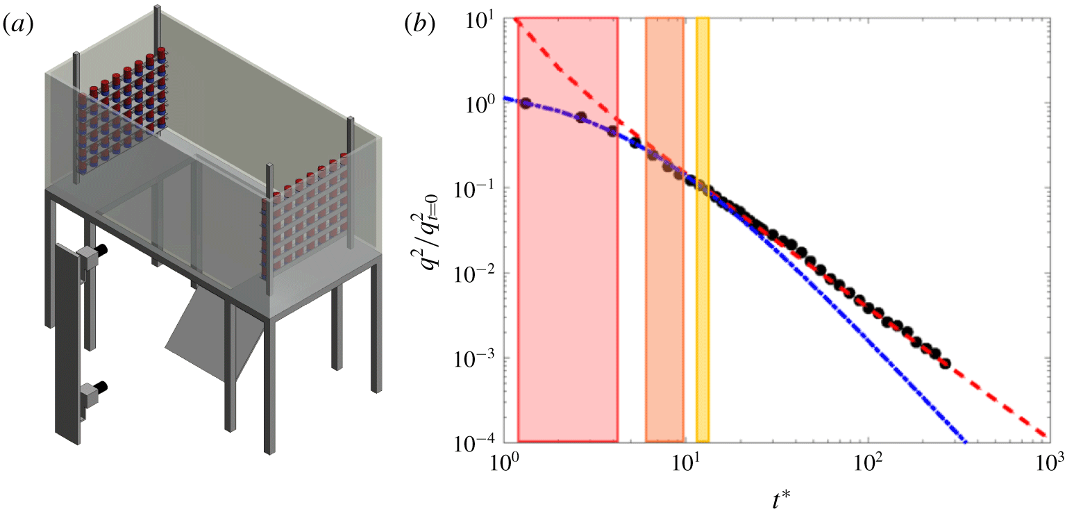
(a) Sketch of the water tank equipped with a co-planar arrangement of random jet arrays. The central region of the frame allows optical access from the bottom; here, through a mirror at  $45^{\circ }$. (b) Time evolution of the turbulent kinetic energy (TKE) during the decay;
 $q^{2}={u_{1}^{\prime }}^{2}+{2u_{2}^{\prime }}^{2}$. Time is made dimensionless with the eddy turnover time at the start of the decay (
 $t_{L}$) as
 $t^{\ast }=t/t_{L}$. Black markers stand for the measured TKE during the natural decay. The dashed-dotted line represents the best fit of the near field and the dashed line the best fit of the far field of the decay. The red, orange and yellow rectangles show the statistical turbulent kinetic energy that the disks will experience during the fall for
 $dt=2$,
 $10$,
 $20~\text{s}$, respectively.

2 Experimental set-up
2.1 Facilities
The experiments were conducted in a RJA facility. The random jet arrays are located in an open glass (bottom and walls) and steel-framed tank of dimensions  $200\times 85\times 100~\text{cm}^{3}$ at a distance of 165 cm from each other. The structure holding the water tank is designed so that the central region of the tank (
 $100\times 90~\text{cm}$) is optically accessible from the bottom. The tank was filled with tap water, of density
 $0.996~\text{g}~\text{cm}^{-3}$, to a height of
 $80~\text{cm}$. The kinematic viscosity was estimated to be
 $1.02\times 10^{-6}~\text{m}^{2}~\text{s}^{-1}$ at room temperature (
 $20\,^{\circ }\text{C}$).
In this facility, turbulence is generated by two facing planes of randomly actuated jet arrays, in the same fashion as in Esteban et al. (Reference Esteban, Shrimpton and Ganapathisubramani2019a). Each plane of jets contains  $48$ bilge pumps (Rule 24, 360 GPH) arranged in a
 $8\times 6$ array as shown in figure 1(a). The pumps take in water radially at their base and discharge it axially via a cylindrical nozzle (
 $1.8~\text{cm}$ inner diameter). Each pump acts as a synthetic jet, in the sense that they only inject momentum into the system, since the pump intake and nozzle are contained within the same volume of fluid. Each plane of bilge pumps is connected to a solid state relay rack SSR-RACK48 equipped with quad-core relays SSR-4-ODC-05. The relays are triggered by transistor–transistor logic (TTL) signals from a Measurement Computing 96 channel digital output card (PCI-DIO96H) controlled by MATLAB. The firing algorithm we employ to force turbulence is the ‘Sunbathing’ algorithm originally proposed in Variano & Cowen (Reference Variano and Cowen2008), and later investigated in Bellani & Variano (Reference Bellani and Variano2013), Carter et al. (Reference Carter, Petersen, Amili and Coletti2016) and Esteban et al. (Reference Esteban, Shrimpton and Ganapathisubramani2019a) among others.
Different test cases were achieved by keeping the disk and fluid density constant but changing the disk thickness  $h$ and diameter
 $D$. All disks were made of aluminium with a density of
 $2.70~\text{g}~\text{cm}^{-3}$, thus the density ratio was fixed at
 $\unicode[STIX]{x1D70C}_{p}/\unicode[STIX]{x1D70C}_{f}=2.7$. The disk material properties, Archimedes number
 $Ar$ and dimensionless moment of inertia
 $I^{\ast }$ are summarized in table 1. The Archimedes number
 $Ar=\sqrt{3/32}U_{g}D/\unicode[STIX]{x1D708}$, which can be defined as a Reynolds number based on the gravitational speed
 $U_{g}=\sqrt{2(\unicode[STIX]{x1D70C}_{p}/\unicode[STIX]{x1D70C}_{f}-1)gh}$, has been recently considered to be one of the true control parameters (see Auguste et al. Reference Auguste, Magnaudet and Fabre2013) since the gravitational speed is known a priori. The dimensionless inertia is the other control parameter,
 $I^{\ast }=I_{p}/\unicode[STIX]{x1D70C}_{f}D^{5}$, where
 $I_{p}$ is the mass moment of inertia about the diameter of the disk. The disks used in this study were manufactured to lie in the (
 $Ar-I^{\ast }$) domain corresponding to the ‘fluttering’ regime first defined in Willmarth et al. (Reference Willmarth, Hawk and Harvey1964) and more precisely in the ‘planar zig-zag’ sub-regime defined in Zhong et al. (Reference Zhong, Chen and Lee2011). Therefore we expect them to describe a highly planar oscillatory motion when released in quiescent flow. This will reduce the variability in the natural descent of the particle, revealing more clearly the effect of background turbulence.
Main geometric and material parameters of the disks that define the Archimedes number ( $Ar$) and the dimensionless moment of inertia (
 $I^{\ast }$), both defined in § 1.1.

In all experiments, the disks were released using a mechanism that employs active suction and is capable of accommodating all disks considered here. When the suction circuit is opened the pressure difference maintaining the particle fixed vanishes and the particle begins its descent through the tank.
2.2 Measurement of the body motion
The location of the disk throughout the descent was measured using a stereoscopic vision system consisting of two digital cameras and diffuse light source, as shown in figure 1. The cameras (JAI GO-5000M USB) were used to capture two views of the falling particle. Careful attention was paid to the camera alignment to make the two views orthogonal for the later digital processing and trajectory reconstruction. One camera recorded the front view of the descend while the other recorded the bottom view of the descend through a mirror at  $45^{\circ }$. The cameras were synchronized and triggered using an external 5 V signal sent from an Arduino. The trajectories were recorded at
 $60$ frames per second and this frame rate was sufficient to resolve the translation motion during all parts of the descent. In each frame the dark particle projection is recorded onto the white background and the position of the particle centre of mass was obtained by locating the geometric centre of each particle projection. The image processing was performed using an in-house script developed in MATLAB, as in Esteban et al. (Reference Esteban, Shrimpton and Ganapathisubramani2018), Esteban, Shrimpton & Ganapathisubramani (Reference Esteban, Shrimpton and Ganapathisubramani2019b). The method to obtain the particle position from the grey-scale image is a threshold based method, where raw images are converted into black and white images after applying a user defined intensity threshold. For the accuracy on the particle location we rely on a stable light intensity during all parts of the trajectory. Commercial LED panels connected to a stable DC power supply were used to back illuminate the field of view. Both LED panels were mounted to cover the complete field of view of both cameras; i.e.
 $60\times 60~\text{cm}$ for the bottom view and
 $60\times 80~\text{cm}$ for the front view. The panels were used at maximum light intensity. Thus, we were able to close the aperture of the camera diaphragm (
 $f.4$), which lead to an increase in the focal depth.
The measured trajectories were smooth, but a polynomial filter of third order and frame length of  $5$ points were used to filter out high frequency noise. Both cameras were always positioned at a relatively small distance from the tank to have a good compromise between field of view and number of pixels per particle diameter. The process followed to obtain the particle centre of mass did not add any uncertainty for the case of a thin disk.
A set of releases of a polylactide (PLA) sphere falling in air was performed to establish limitations on the accuracy associated with the drop mechanism as well as the measurements taken by the cameras and to account for image distortion from the lens. The variance in the landing position was a measure of the uncertainty of the system, being two to three orders of magnitude smaller than the sphere diameter. The magnitude of the uncertainty is in accordance with similar systems found in the literature (Heisinger, Newton & Kanso Reference Heisinger, Newton and Kanso2014).
2.3 Methods
In all experiments, the disk was released with the same initial conditions ( $V_{t=0}=0$,
 $\unicode[STIX]{x1D703}_{t=0}=0\pm 0.1^{\circ }$, where
 $\unicode[STIX]{x1D703}$ is the particle inclination angle) using a mechanism that employs active suction. This system was part of a rigid frame attached to the top of the water tank, with the suction cup mounted flushed into a submerged flat plate with adjustable inclination angle to ensure that the particle initial conditions were the same in all realizations. The disks were dropped from a height sufficiently large (
 $80~\text{cm}$) to allow the falling regime to fully develop during the observation. This vertical path corresponds to
 $80$,
 $64$ and
 $53$ disk diameters for the particles investigated. Each disk was released
 $50$ times in quiescent flow to establish the dynamics of the motion without the influence of background turbulence.
The determination of the distance at which the particle motion is not influenced by the initial transient dynamics is non-trivial. Here, the term ‘saturated path’ stands for the section of the trajectory for which the statistics of the motion are independent of the vertical distance  $z$. Churst et al. (Reference Churst, Bouchet and Dusek2013) performed simulations of an infinitely thin disk with
 $I^{\ast }=3.12\times 10^{-3}$ and
 $Ga=300$ and showed that it reached a ‘saturated path’ at a vertical distance of
 ${\approx}60D$ from the release point, whereas Heisinger et al. (Reference Heisinger, Newton and Kanso2014) showed experimentally that for disks with
 $I^{\ast }\approx 3\times 10^{-3}$ and
 $Ga\approx 4180$, the disk trajectory was saturated after a distance of
 $7D$. Here the dimensionless moment of inertia of the disks is even higher than in Heisinger et al. (Reference Heisinger, Newton and Kanso2014), with
 $I^{\ast }\approx 6-8\times 10^{-3}$ and
 $Re\approx 1000{-}2300$ (or equivalent Galileo number
 $Ga=1.15-2.12\times 10^{4}$) and we observed that after a vertical distance of
 $7D$ from the release point the particle trajectory was unaffected by the transient dynamics (in the quiescent case). Thus, a distance of
 $7D$ is given to the particle to accommodate to the fall before the trajectories are analysed.
As discussed in Heisinger et al. (Reference Heisinger, Newton and Kanso2014), the bottom of the tank influences the landing position of the particle due to hydrodynamic interactions and the particle persistent motion once it is flat on top of the glass surface. To overcome these influences we do not process the particle trajectory once it reaches a distance of  $2D$ from the bottom of the tank. Thus, we save trajectory sections that go from
 $7D$ from the top (corresponding to a location were the particle trajectory is at a saturated state) to
 $2D$ from the bottom (unperturbed by the glass surface). After the quiescent cases, each disk was released in a turbulent environment (200 realizations per case). To recreate turbulent scenarios with similar flow characteristics, the water tank was actively stirred using both RJAs for a period of 5 min until the turbulence level reached a statistically stationary state. Then, all pumps were turned off simultaneously and a disk was released after a given waiting time (
 $dt$). The reader is referred to Esteban et al. (Reference Esteban, Shrimpton and Ganapathisubramani2019a) for specific details on the temporal decay of turbulence in the tank. The scenarios considered in this study are
 $dt=2$,
 $10$ and 20 s. These three waiting times allowed us to study the descent style of each particle at different levels of background turbulence intensity and to investigate how this affects the descent mode of disks with different dimensionless numbers (
 $Ga$,
 $I^{\ast }$). The turbulence intensity in the tank at the start of the fall is chosen to illustrate the overall effect of background turbulence on the dynamics of the disk. However, while the disk falls through the tank it experiences a homogeneous decaying (in time) turbulent flow which could be understood as a mild stratified turbulent flow. The variation of the turbulence intensity is highest for the shortest waiting time (
 $dt=2~\text{s}$) and this corresponds to approximately
 $25\,\%$ from top to bottom of the tank. The variation of the turbulence intensity reduces to approximately
 $12\,\%$ for
 $dt=10~\text{s}$ and
 $3{-}4\,\%$ for
 $dt=20~\text{s}$.
3 Falling style
3.1 Falling style in quiescent flow
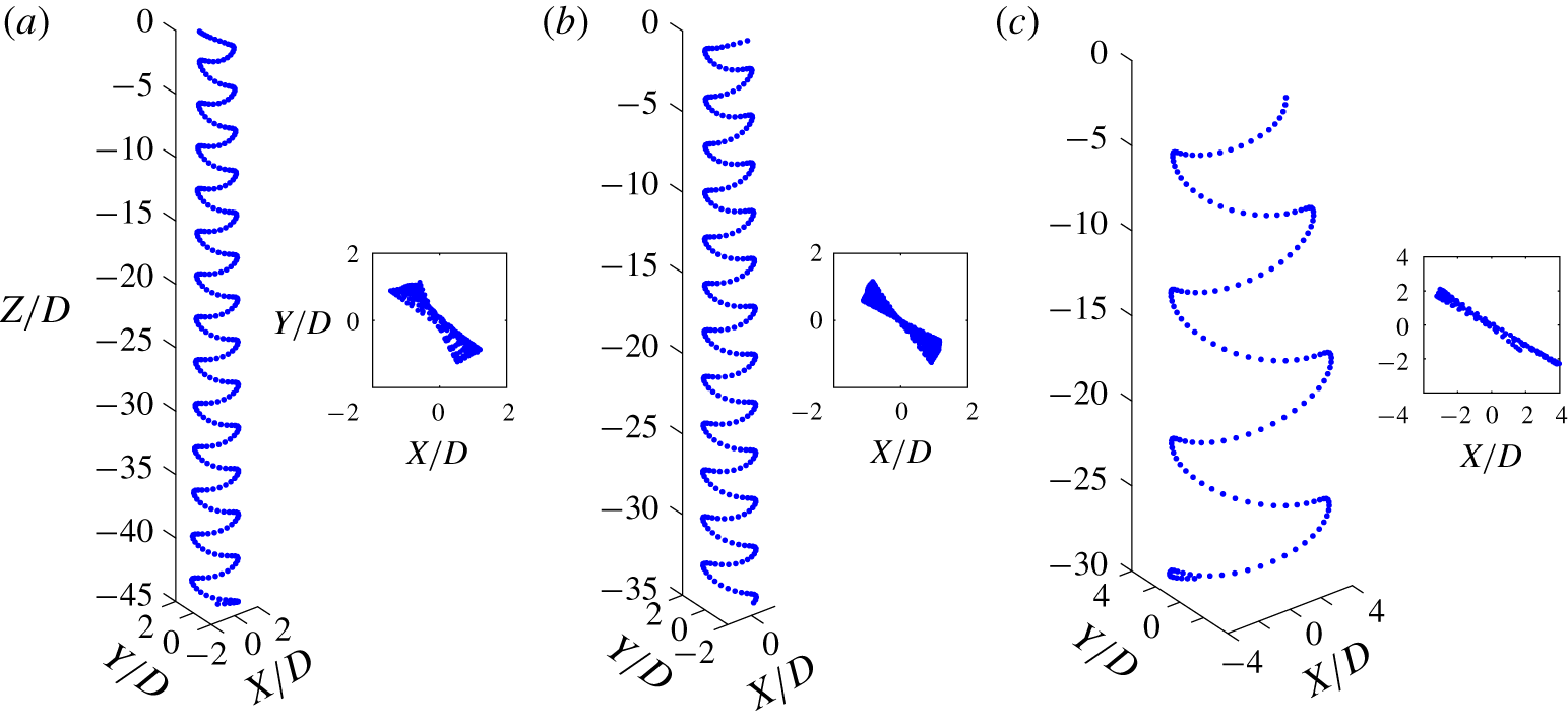
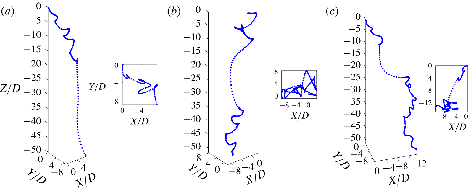
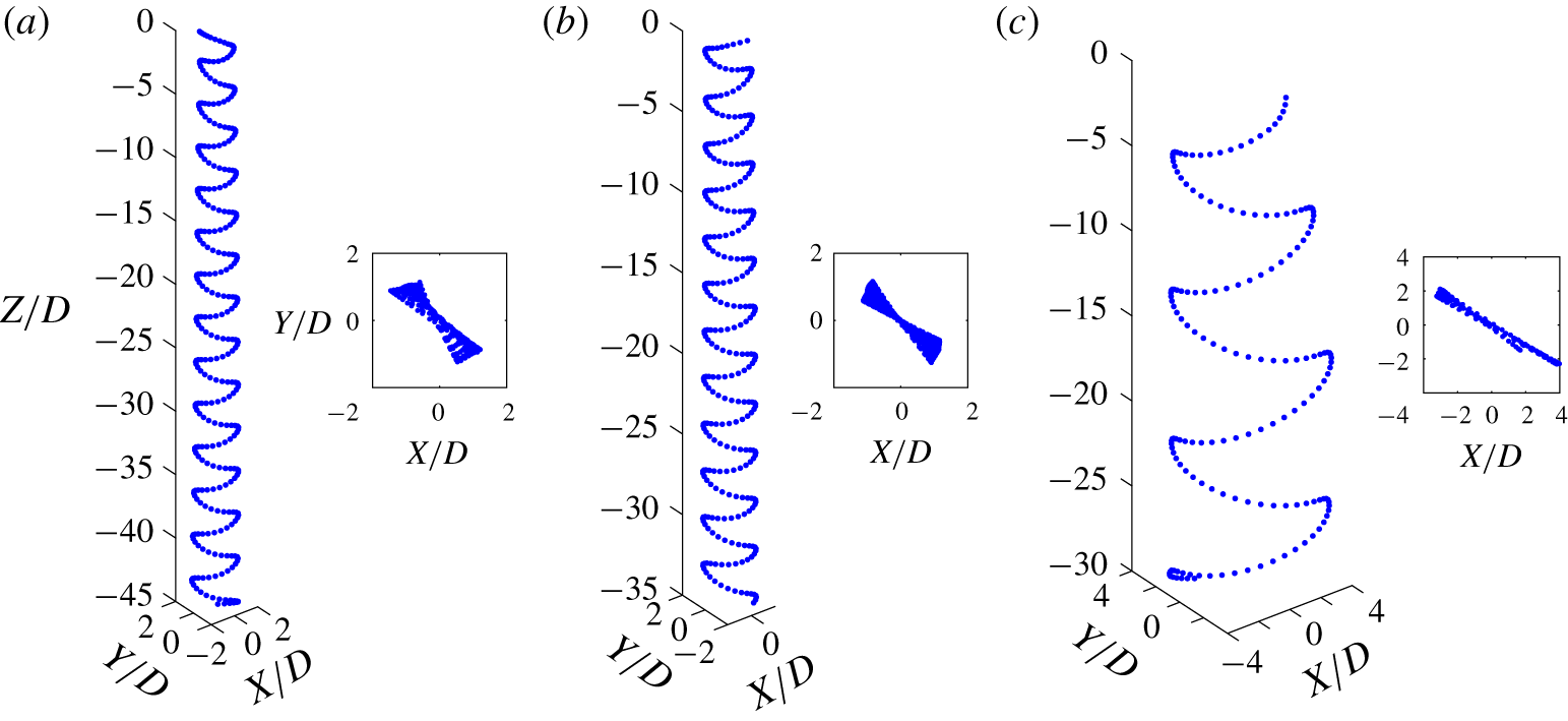
The three disks show a highly planar descent motion, as expected from the magnitudes of the Archimedes number and dimensionless moment of inertia shown in table 2. Also, from the mean descent velocity of the disks we corroborate that they lie within the  $Re-I^{\ast }$ domain corresponding to the ‘planar zig-zag’ identified by Zhong et al. (Reference Zhong, Chen and Lee2011) and later investigated by Lee et al. (Reference Lee, Su, Zhong, Chen, Zhou and Wu.2013) and Zhong et al. (Reference Zhong, Lee, Su, Chen, Zhou and Wu.2013). A highly periodic motion under quiescent flow is of particular interest in this study since it will allow us to differentiate the natural frequency of the particle from the frequencies induced by turbulence. Figure 2 shows a section of the descent trajectory for the three disks investigated, where one can observe very small deviations from the idealized planar motion. The trajectories measured are in very good agreement with experimental and numerical results found in the literature (Auguste et al. Reference Auguste, Magnaudet and Fabre2013; Churst et al. Reference Churst, Bouchet and Dusek2013; Lee et al. Reference Lee, Su, Zhong, Chen, Zhou and Wu.2013).
Three-dimensional trajectory reconstruction of sections of the disk descent in quiescent flow. (a) Disk no. 1, (b) disk no. 2 and (c) disk no. 3. The particle dispersion is normalized with the disk diameter.
Reconstructed 3-D trajectories and ( $X,Y$) planar projection for disk no. 1 released after of waiting time
 $dt=2$. The particle dispersion is normalized with the disk diameter.

3.2 Falling style in turbulence
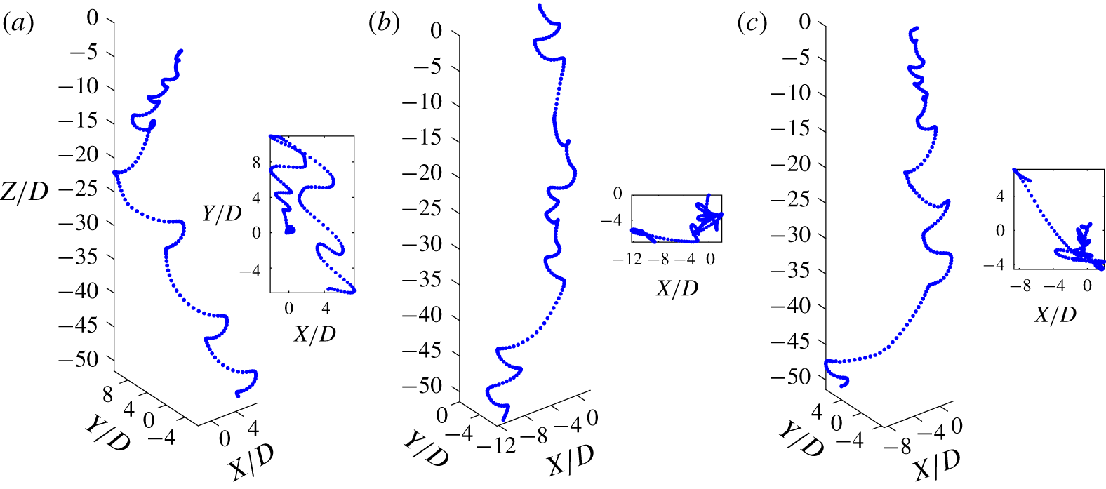
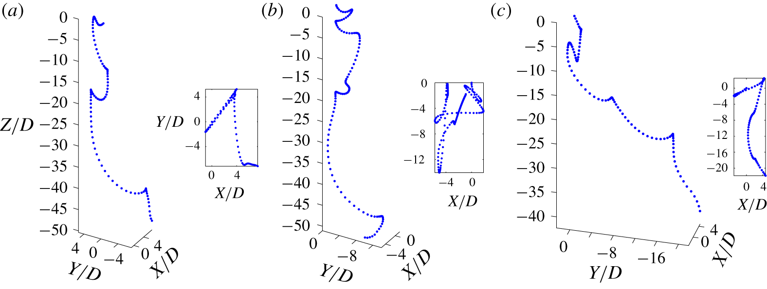
Sample particle trajectories falling under the effect of background turbulence are plotted in figure 3 to allow visual comparison with the trajectories of disks falling in quiescent flow (figure 2), where a few interesting events are observed for the cases presented. In figure 3(a) one can observe that the disk, strongly influenced by large turbulent structures in the flow, can describe low frequency oscillations in the  $X{-}Y$ plane, leading to a preferential lateral motion during sections of the descent. More precisely, we observe that the disk, while fluttering, moves laterally about
 $10D$ in one direction to later reverse the lateral motion during the second half of the descent. At the same time, one can observe in all figures very long gliding sections during the descent that increase severely the particle dispersion (distance between the particle release point and the particle local position). Similarly, the local slope of the gliding sections (and therefore particle nutation angle
 $\unicode[STIX]{x1D703}$) is considerably higher than in the case of quiescent flow. However, this does not occur after every turning section but depends on the local flow around the particle.
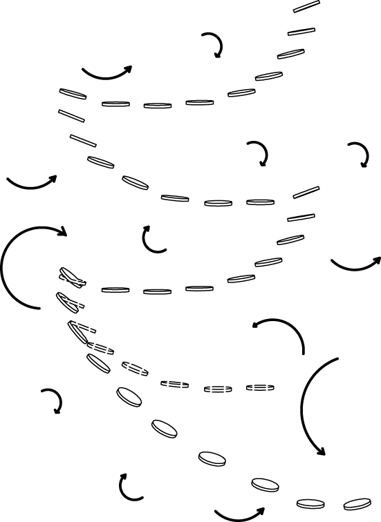
We believe that the long gliding sections are caused by the flow moving locally in the same direction as the natural motion of the particle and therefore enhancing the particle flutter. However, these long gliding events can be attenuated during the descent and be substituted by ‘standard’ fluttering, as in figure 3(b) for the trajectory section corresponding to  $-20<Z/D<-30$. On the other hand, we believe that trajectory sections of high nutation angle are governed by the particle–turbulence interaction during the previous turning event. Thus, when a turbulent structure destabilizes the particle at the turning point, it induces a higher particle nutation angle and it strongly modifies the particle local descent (until the new turning point is reached), as sketched in figure 4.
Sketch of a disk falling under the effect of turbulence to illustrate how turbulent structures destabilize the particle near the turning points. The particle with dashed contours represents the particle trajectory in quiescent flow.

Reconstructed 3-D trajectories and  $X{-}Y$ planar view released after of waiting time
 $dt=2$. The particle dispersion is normalized with the disk diameter. (a) Disk no. 1, (b,c) disk no. 2.

Reconstructed 3-D trajectories and ( $X,Y$) planar projection for disk no. 3 released after of waiting time
 $dt=2$. The particle dispersion is normalized with the disk diameter. All three panels represent different realizations of disk no. 3 after the same waiting time.

In some rare instances we observe the particle to describe a complete ‘tumbling event’ in between successive gliding sections. This can be seen in figure 3(c) at approximately the vertical position of  $Z/D\approx -35$. In these situations we believe that the particle inertia overcomes the fluid resistance during the turning point due to an increase in the relative velocity, leading to a complete particle revolution.
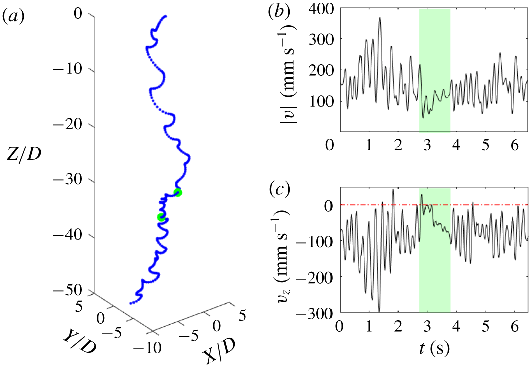
‘Slow’ event during the descend of disk no. 1 under turbulence effects released after a waiting time  $dt=2$. (a) Reconstructed 3-D trajectory with the dispersion normalized with the disk diameter, green dots show the start and end of the ‘slow’ subsection. (b,c) Time evolution of the particle speed and particle descent velocity, the green shaded region showing the ‘slow’ subsection.

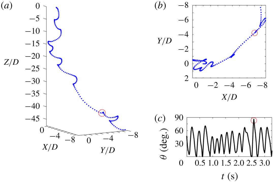
Similarly, figure 5 and figure 6 show other particle–fluid interactions leading to ‘fast’ descents. One can observe that in some cases the particle reaches a very high incidence angle right after the turning event, leading to a very fast descent with the disk leading edge aligned with the descent motion (figure 5a). This can be observed more easily when the particle 3-D motion is plotted together with the temporal particle nutation angle ( $\unicode[STIX]{x1D703}$) and the top view of the complete trajectory. In figure 8, a trajectory containing a fast tumbling event is plotted using this layout with a red marker indicating the location of the tumbling event in all three panels. One can observe that, during the tumbling event, the measured particle nutation angle in figure 8(c) reaches a maximum of
 ${\approx}90^{\circ }$ (which is not fully captured due to time resolution limitations). Similarly, the particle planar motion is not reversed after that event (see figure 8b) and the frequency of the descent velocity fluctuations remains nearly the same (not shown here).
Fast tumbling event during the descend of disk no. 1 under turbulence effects released after a waiting time  $dt=2$. The red marker shows the location of the tumbling event. (a) Reconstructed 3-D trajectory with the dispersion normalized with the disk diameter. (b) Reconstructed top view of the trajectory with the dispersion normalized with the disk diameter showing that the
 $X{-}Y$ disk direction before and after the event remains nearly the same. (c) Time evolution of the particle nutation angle (
 $\unicode[STIX]{x1D703}$) during the descent.

Another interesting descent event observed is the slow tumble motion, as in figure 5(b). In this situation, the disk starts a standard gliding section but instead of the usual descent velocity attenuation before reaching the extreme of the planar oscillation, the descent velocity keeps increasing and the disk undergoes a complete rotation; this event taking approximately  $25D$ in the vertical direction. We believe this might be caused by the particle interaction with a large turbulence structure that destabilizes the particle steadily during the gliding section. We only observed this effect for disk no. 1 and disk no. 2 and we believe that these large turbulence structures might not be strong enough to overcome particle inertia for disk no. 3 (particle with higher
 $I^{\ast }$). In § 4.1 we address in more detail the particle–turbulence scale ratios and we propose an explanation for the motions observed. In figure 6 one can observe some of the fast events described before excepting disk no. 3. These are a combination of high and low frequency oscillations in figure 6(a,b) and tumbling events in figure 6(c), as if the particle belongs to another region of the
 $Re-I^{\ast }$ regime map.
Figure 7 shows a sample trajectory of disk no. 1 that contains a trajectory section with very low velocity magnitude. In fact, the velocity magnitude remains smaller than the particle mean descent velocity in quiescent flow for a time interval of approximately  $1~\text{s}$, which corresponds to two particle periods in quiescent flow according to the dominant frequency of the descent velocity. This magnitude was estimated by applying fast Fourier transform to the descent velocity signal and it was later used to plot figure 9. From the evolution of the speed and the descent velocity (figures 7b and 7c respectively) one can observe that this event occurs in between two sections of ‘standard’ descent. This highlights the influence of turbulence in the local dynamics of the disk and shows that certain particle–turbulence configurations can lead to a severe reduction of the descent velocity and total speed for long durations. These trajectories, with ‘slow’ and ‘fast’ events contained within a single descent illustrate the complexity of the disk trajectories when background turbulence is introduced.
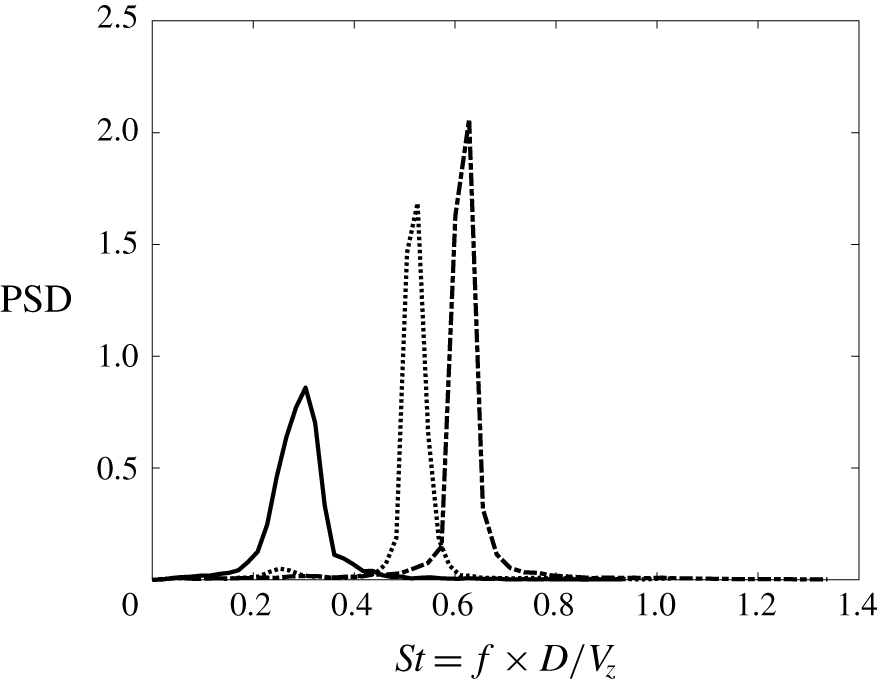
Normalized power density spectrum as a function of the Strouhal number. The peak in the spectrum is used to identify the characteristic particle Strouhal number. The dotted line represents no. 1, the dashed-dotted line disk no. 2 and the solid line disk no. 3, all descending in quiescent flow.

4 Descent velocity
In this section we report on the changes in descent velocity of the disks with the addition of background turbulence. The descent of each of the disks in quiescent flow is always used as the baseline to compare particle descents.
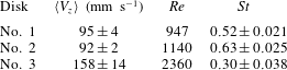
Values of the mean descent velocity of all realizations ( $\langle V_{z}\rangle$), particle Reynolds number (
 $Re$) and Strouhal number (
 $St=f\cdot D/V_{z}$) based on the dominant frequency of the descent velocity in quiescent flow.
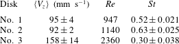
The mean descent velocity of the disks in quiescent flow are shown in table 2 together with the standard deviation from the 50 independent realizations. We observe a reduction in mean descent velocity from disk no. 1 to disk no. 2. This is due to the stronger contribution of the hydrodynamic forces acting on the extended surface area as compared with the increase in gravitational force from the change in particle mass.
We compute the power spectral density from the fluctuations of the descent velocity signal and observe that the velocity descent is governed by one characteristic frequency ( $f$). The Strouhal number is obtained from the dominant frequency of the velocity fluctuations, the disk diameter and the measured mean descent velocity, as
 $St=fD/V_{z}$. The results in figure 9 are in good agreement with previous numerical work by Auguste et al. (Reference Auguste, Magnaudet and Fabre2013), where they showed that the relation between the Strouhal number and dimensionless moment of inertia followed
 $St\sim I^{\ast -0.36}$ (see table 1 and 2 for
 $I^{\ast }$ and
 $St$ data respectively). We believe that the wider shape of the power spectral density for disk no. 3 might be caused by the relative shorter length of the signal, leading to stronger deviations in the frequency data per particle trajectory, as already observed in the deviation of the mean descent velocity in table 2.
4.1 Effect of background turbulence
Here, we compare the descent velocity of disks falling through background turbulence with the results previously reported. We initially observed that the falling styles of the disks vary dramatically during individual descents and also in different realizations. To capture the wide variability of the descent style we analyse  $200$ independent realizations for each disk and flow condition. We consider three different turbulent conditions that correspond to different points in time during the free decay of the turbulence generated. The turbulent kinetic energy, here expressed as
 $q^{2}=u_{1}^{2}+2u_{2}^{2}$ due to the symmetry of the facility (see Esteban et al. Reference Esteban, Shrimpton and Ganapathisubramani2019a), at these points during the decay is shown in figure 1(b). The red, orange and yellow colours in figure 1(b) will be used in the following part of the discussion to represent quantities at the three waiting times considered.
The ratio between the descent velocity of the particles in quiescent conditions (defined as  $\unicode[STIX]{x1D70F}_{p}g$ for spherical particles) and the mean velocity fluctuations has been extensively used to determine the change in settling speed of inertial particles (Nielsen Reference Nielsen1993; Good, Gerashchenko & Warhaft Reference Good, Gerashchenko and Warhaft2012; Good et al. Reference Good, Ireland, Bewley, Bodenschatz, Collins and Warhaft2014; Byron et al. Reference Byron, Einarsson, Gustavsson, Voth, Mehlig and Variano2015). Here, the gravitational velocity (
 $\unicode[STIX]{x1D70F}_{p}g$) is substituted by the descent velocity in quiescent flow
 $\langle V_{z}\rangle$ given in table 2, due to the difficulties associated with defining an appropriate particle relaxation time for particles with strong secondary motions. Thus, the ratio
 $\langle V_{z}\rangle /u^{\prime }$, where
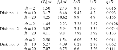
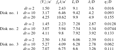
 $u^{\prime }$ stands for the r.m.s. of the turbulence velocity fluctuations, is included in table 3 for each particle and flow condition tested. We also include the ratio between the dominant fluttering frequency of the particle in quiescent flow and the turbulent frequency based on the Taylor length scale (
 $\unicode[STIX]{x1D706}$) and the r.m.s. of the turbulence velocity fluctuations (
 $u^{\prime }$). One can understand this ratio as the number of fluttering periods that the particle performs before encountering a turbulent eddy of scale
 $\unicode[STIX]{x1D706}$.
Values of the particle–turbulence velocity ratio ( $\langle V_{z}\rangle /u^{\prime }$), frequency ratio (
 $f_{q}\unicode[STIX]{x1D706}/u^{\prime }$) and main turbulent structure to particle diameter ratios, where
 $f_{q}$ stands for the dominant fluttering frequency in quiescent flow,
 $L$ for the integral length scale,
 $\unicode[STIX]{x1D706}$ for the Taylor length scale and
 $\unicode[STIX]{x1D702}$ for the Kolmogorov length scale.
For spherical particles, Good et al. (Reference Good, Ireland, Bewley, Bodenschatz, Collins and Warhaft2014) found that turbulence enhances the settling of particles for particle gravitational velocities smaller than the turbulence velocity fluctuations ( $\unicode[STIX]{x1D70F}_{p}g/u^{\prime }<1$), whereas the settling is inhibited when the turbulence velocity fluctuations are smaller than the particle gravitational velocities (
 $\unicode[STIX]{x1D70F}_{p}g/u^{\prime }>1$). However, the change in mean descent velocity might not follow the same trend when aspherical particles with strong secondary motion are considered. Here, the r.m.s. of the velocity fluctuations never exceeds the value of the particle descent velocity in quiescent flow and represents a velocity fluctuation of approximately
 $0.7\langle V_{z}\rangle$ for the shortest waiting time (
 $dt=2~\text{s}$). Therefore, being in the
 $\unicode[STIX]{x1D70F}_{p}g/u^{\prime }>1$ scenario, particles should always fall more slowly than in quiescent flow (if the trend for spherical particles is followed).
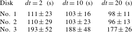
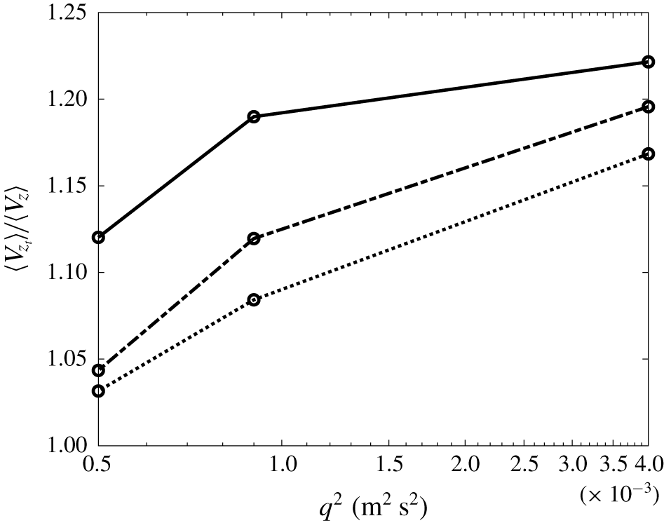
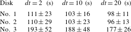
Figure 10 shows the ratio of the mean descent velocity of the particles under turbulent conditions to their velocity in quiescent flow. Contrary to what one would expect for spherical particles, the mean descent velocity of the disks increases significantly as the turbulence intensity in the facility does so. The standard deviation of the mean descent velocity for the  $200$ trajectories per case is also shown in table 4, and this corresponds to approximately
 $25\,\%$ of the mean descent velocity magnitude for the
 $dt=2$ case. We also observe that the particle descent velocity increases with the probability of encountering an eddy of equivalent size (
 $\unicode[STIX]{x1D706}\approx D$) per swing. Thus, disk no. 3 (which encounters a turbulent eddy of size
 $\unicode[STIX]{x1D706}$ more frequently than the other disks) shows the highest relative descent velocity. We believe this hypothesis agrees well with the results shown in Tom & Bragg (Reference Tom and Bragg2019), where they showed that the flow scales for which particle inertia becomes small are the ones responsible for the enhancement of the particle-settling velocity (
 $St>1$) under turbulent conditions.
Values of the particle descent velocity for the three flow conditions at different waiting times during the turbulence decay. The mean descent velocity and the standard deviation of the  $200$ realizations per case are shown. Units are
 $\text{mm s}^{-1}$.
Evolution of the mean descent velocity of inertial disks under turbulent conditions ( $\langle V_{z_{t}}\rangle$) as a function of the turbulence intensity. The descent velocity of the particles is normalized using the mean descent velocity of the particle in quiescent flow (
 $\langle V_{z}\rangle$). Dotted line stands for disk no. 1, broken line for disk no. 2 and solid line for disk no. 3.

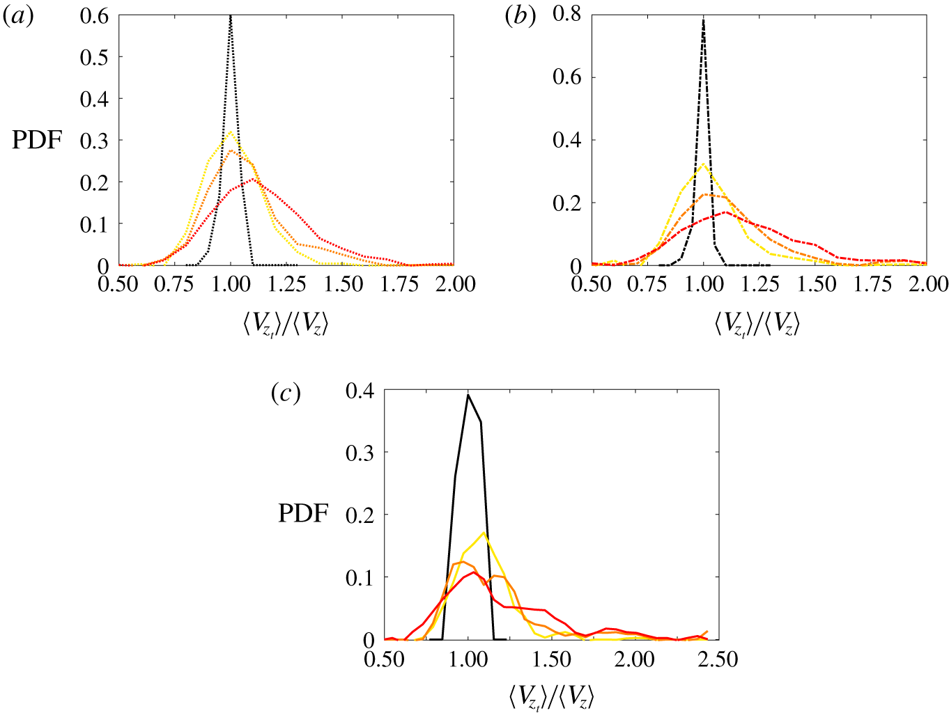
Figure 11 shows the data corresponding to the  $200$ trajectories per disk got (a) disk no. 1, (b) disk no. 2 and (c) disk no. 3 and flow configurations (
 $dt=2~\text{s}$ in red,
 $dt=10~\text{s}$ in orange,
 $dt=20~\text{s}$ in yellow and quiescent flow in black) in the form of probability density functions of the mean descent velocity per trajectory. As expected from the results in figure 10, these figures show that as the turbulent kinetic energy increases all three disks exhibit fast descents more often than in quiescent flow. In some extreme instances, the mean descent velocity along a single trajectory can double the descent velocity of the disk in quiescent flow; and this is observed for the three disks under strong background turbulence (red lines). However, one can also observe that the tails of the red lines in figure 11 also become wider towards the slower side of the velocity range.
Probability density function (PDF) of the ratio of the measured mean descent velocity for disks falling in background turbulence to the measured mean descent velocity of the disks in quiescent flow. The colours of the PDF stand for flow configurations: black for quiescent flow, yellow for  $dt=20$, orange for
 $dt=10$ and red for
 $dt=2$. (a) Disk no. 1, (b) disk no. 2 and (c) disk no. 3.

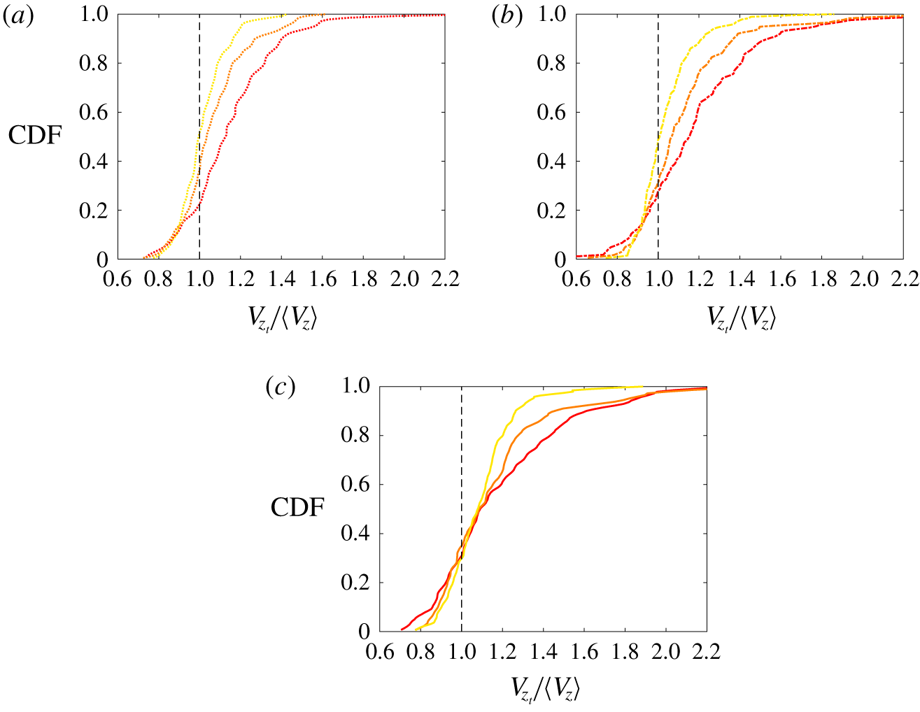
The same results are shown as a cumulative density function (CDF) in figure 12 to emphasize the effect of turbulence intensity on the mean descent of the particles. In these figures one can observe that, independently of the particle characteristics and waiting time, the descents that are slower than the mean descent in quiescent flow (left of the vertical broken line) correspond to approximately  $20\,\%$ of the total cases. Also, it is interesting to highlight that the region of overlap in the CDFs increases with increasing particle Archimedes number (
 $Ar$). This suggests that as
 $Ar$ increases the particle might be less sensitive to flow perturbations. However, we hypothesize that if these perturbations occur close to the turning point of the particle (when the particle inertia is at a minimum), the flow perturbations can significantly change the particle angle of attack; leading to steeper gliding sections with higher settling velocity.
Cumulative density function of the mean descent velocity normalized with the mean descent velocity of the disks in quiescent flow. The colours of the CDF stand for flow configurations: yellow for  $dt=20$, orange for
 $dt=10$ and red for
 $dt=2$. (a) Disk no. 1, (b) disk no. 2 and (c) disk no. 3.

In the following section we investigate ‘fast’ and ‘slow’ trajectories to see whether the change in descent velocity is associated with a change in falling style.
5 Flutter frequency and descent velocity
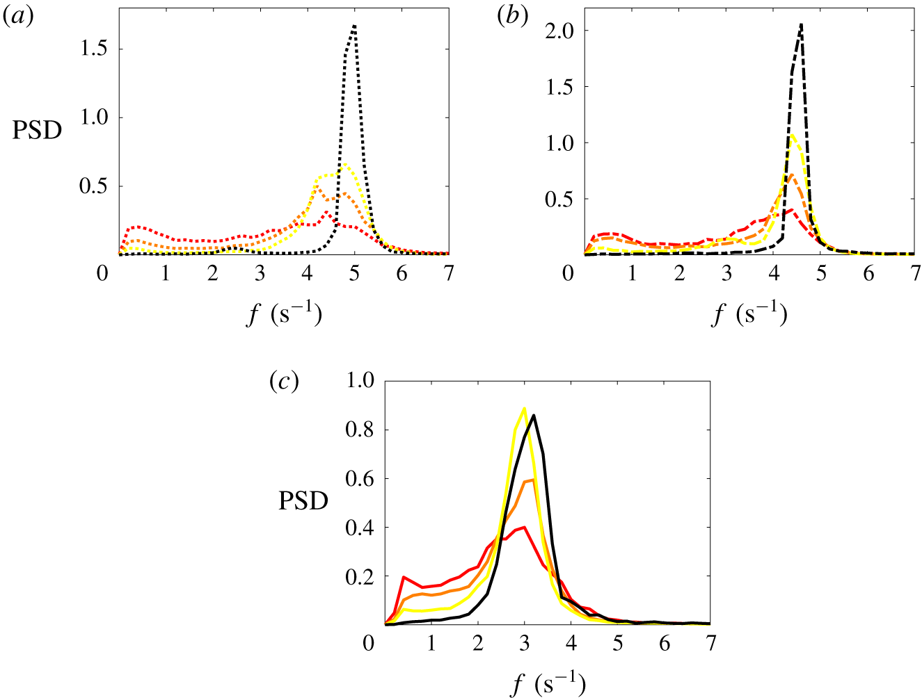
In this section we investigate whether we can establish a connection between the dominant frequency of the vertical velocity fluctuations and the mean descent velocity along the particle trajectory. In order to tackle this question, we analyse the frequency content of the descent velocity signal as in the quiescent flow case. Thus, we plot the mean power spectral density (PSD) of all trajectories under the same flow conditions and compare it with the data obtained for the case of quiescent flow. Figure 13 shows the frequency content of the descent velocity signal for the three disks in separate panels. One can observe that the oscillatory frequency of all three disks in quiescent flow (black line) is maintained independently of the strength of the background turbulence. However, as turbulence increases and interacts more intensely with the particle, the relative strength of the oscillatory frequency in quiescent flow is reduced and the energy content is transferred to smaller frequencies. Interestingly, one can observe that the power spectral density of disk no. 1, that is the particle with higher dimensionless inertia (figure 13c), happens to be less affected as the turbulent kinetic energy increases, whereas for disks no. 1 and no. 2 (figure 13a,b, respectively) a very similar trend is observed.
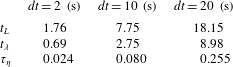
Values of the integral time scale ( $t_{L}$), Taylor length scale (
 $t_{\unicode[STIX]{x1D706}}$) and Kolmogorov length scale (
 $\unicode[STIX]{x1D70F}_{\unicode[STIX]{x1D702}}$) for the three flow conditions. Units in seconds.
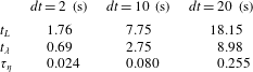
Another important feature observed in the PSDs is that the frequency content not only becomes wider, but also changes shape; and a highly energetic frequency at approximately  $f\approx 0.5~\text{Hz}$ is observed in all cases. This turbulence-induced frequency does not correspond to the characteristic frequency of any of the flow scales considered in table 5. In fact, we believe that for these particle–flow configurations the flow is not entirely responsible for the particle oscillation at
 $f\approx 0.5~\text{Hz}$ but that it only destabilizes the particle, acting as a trigger mechanism that leads to the long gliding sections of the descent.
Normalized power spectral density of the velocity fluctuations in the vertical direction. The colours of the PSDs stand for flow configurations: black for quiescent flow, yellow for  $dt=20$, orange for
 $dt=10$ and red for
 $dt=2$. (a) Disk no. 1, (b) disk no. 2 and (c) disk no. 3.

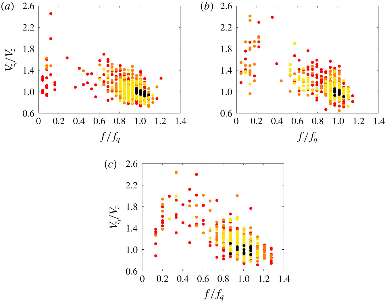
We hypothesize that the severe changes in the mean descent velocity of the particle and the modulation of the descent velocity frequency content are associated with different types of turning events. Therefore, in the following analysis we identify ‘fast’ and ‘slow’ trajectories based on the mean descent velocity to examine the similarity of the characteristic falling style and frequency content.
Mean descent velocity of disks in turbulent flow as a function of the dominant frequency observed in the fluctuations of the descent velocity. Velocity and frequency are normalized with the values of the quiescent cases, given in table 2. The colours in the scatter plot stand for flow configurations: black for quiescent flow, yellow for  $dt=20$, orange for
 $dt=10$ and red for
 $dt=2$. (a) Disk no. 1, (b) disk no. 2 and (c) disk no. 3.

To verify the above hypothesis, we first show the descent velocity of each trajectory as a function of the dominant frequency of the descent velocity fluctuations. Here, the dominant frequency and mean velocity are normalized with the values obtained from the quiescent case. Figure 14 shows the aforementioned relation for the three waiting times (using the colours in figure 1b) and the quiescent case in black as a baseline. The results of disks no. 2, no. 2 and no. 3 in figures 14(a), 14(b) and 14(c), respectively, show that trajectories with higher descent velocity than the quiescent case are more likely to describe small frequency oscillations. In contrast, trajectories with smaller mean descent velocity are shown to describe slightly higher frequencies than the natural frequency in quiescent flow. Interestingly, the frequency of the particle descent velocity fluctuations never exceeds  $1.3f_{q}$ independent of the flow condition, where the sub-index
 $q$ denotes a quiescent magnitude. This suggests that particles might be filtering all turbulence fluctuations with time scales smaller than
 $1/1.3f_{q}$; but more detailed experiments are needed to draw strong conclusions along these lines. Also, one can observe that as turbulence intensity increases, the spread of the data becomes more pronounced, leading to both very fast and considerably slow descents.
Now we can also group the trajectories according to the mean descent velocity of the particle, and independently of the waiting time prior to the particle release. The velocity threshold that we use for ‘slow’ trajectories is the mean descent velocity of each disk in quiescent flow and this represents approximately 20 % of the trajectories under turbulence effects. Then, to compare a similar number of trajectories, we group the 20 % of the fastest descents for each particle. This represents a velocity threshold of approximately  $V_{z}=1.3,1.4,1.5\,V_{q_{z}}$ for disks no. 1, no. 2 and no. 3, respectively. Thus, we obtain two groups of trajectories per disk; i.e. ‘slow’ and ‘fast’ trajectories and the groups under this new classification are now investigated following the same procedure as above.
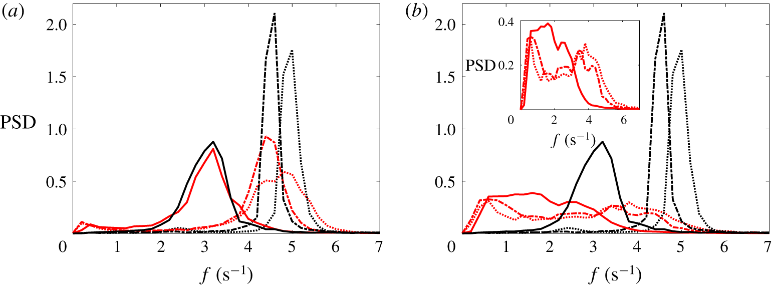
Normalized power spectral density of the descent velocity fluctuations. The red lines stand for the conditional averaged trajectories ‘slow’ trajectories in (a), ‘fast’ trajectories in (b). The black lines correspond to the data for quiescent flow. The line styles represent the three different particles; dotted line for disk no. 1, broken line for disk no. 2 and solid line for disk no. 3.

Figure 15 shows the normalized power spectral density of the grouped trajectories. It is clear that the slow trajectories of high inertia particles resemble their quiescent counterpart (solid line). As the inertia is reduced, the turbulence starts to play a role and tends to increase the amplitude of low frequency motions. Yet, the peak frequency for these ‘slow’ events is very similar to the quiescent case. On the contrary, ‘fast’ trajectories (red lines in figure 15b) show severe differences in the frequency content of the descent velocity signal, where low frequency motions appear to dominate the descent. It is also interesting to note the bimodal energy distribution observed for disks no. 1 and no. 2 in the inset of figure 15(b). The high frequency peak of these distributions is much more attenuated and is located at a lower frequency that in quiescent flow ( $3.8$ and
 $3.4~\text{Hz}$ for disks no. 1 and no. 2 respectively), whereas the low frequency peak is in both cases at
 $0.6~\text{Hz}$, as first estimated from figure 13 for all trajectories recorded. These results show that two different dominant frequencies can coexist in ‘fast’ trajectories; the natural frequency of oscillation of the disk in quiescent flow and the ‘turbulence-induced frequency’. On the other hand, for the case of disk no. 3 the contribution of the two dominant frequencies are overlapped, forming a wider unimodal energy distribution, and therefore the two peaks are not as easy to identify as in the former cases.
6 Discussion and concluding remarks
The free fall motion of thin disks released in homogeneous turbulence was investigated experimentally. We used a stereoscopic vision technique to extract 3-D trajectory information on the disk falling style, mean descent velocity and the frequency content of the velocity fluctuations.
Contrary to what was numerically and experimentally found for spherical particles in Kawanisi & Shiozaki (Reference Kawanisi and Shiozaki2008) and later confirmed experimentally in Good et al. (Reference Good, Ireland, Bewley, Bodenschatz, Collins and Warhaft2014), finite-size inertial disks show an increase in the descent velocity for turbulence velocity fluctuations smaller than the particle descent velocity in quiescent flow ( $\langle V_{z}\rangle /u^{\prime }\approx [1.45-7]$). However, we found that this velocity ratio is not the only parameter responsible for the velocity enhancement since disks show a different relative velocity increase for similar velocity ratios. In contrast, we found that the enhancement of descent velocity is linked to the probability of the particle finding a turbulent eddy of similar size per swing. Thus, disks falling under background turbulence fall faster in scenarios where the natural frequency of the particle is of the same order of magnitude as the frequency of the flow at the same length scale.
We believe small eddies acting on the particle cancel out each other, whereas large eddies do not have enough local strength to induce a severe change in the particle tilt angle. However, turbulent eddies of equivalent size to the particle diameter might be the ones responsible for the destabilization of the disk close to the turning point (where the particle carries less inertia). In this scenario, the disk can be orientated at a higher angle of attack that leads to a new ‘stable’ configuration where the particle experiences a severe enhancement of the local descent velocity. Thus, we believe that the physical mechanisms responsible for the velocity enhancement greatly differ from the ones previously observed for heavy spherical particles (see Bec et al. (Reference Bec, Homann and Ray2014) and Good et al. (Reference Good, Ireland, Bewley, Bodenschatz, Collins and Warhaft2014) among others). We also believe that particle dimensionless inertia plays an important role in the particle stability and therefore in the descent velocity under turbulent conditions. This will be further investigated in the future.
We also found that disks under strong turbulence effects may describe characteristic features of descent styles associated with other regions of the  $Re-I^{\ast }$ regime map, such as the tumbling motions reported. More interestingly, we observed a wide range of descent events that are not present in the quiescent flow scenario, as the ‘slow tumbling’ event where the particle performs a complete revolution within a very long vertical distance (
 ${\approx}25D$) or the ‘levitating’ event for which the particle barely descends for intervals of approximately two oscillatory periods in quiescent flow while describing fluttering type oscillations.
We also found that the motion of the disks seems to be unaffected by turbulence structures with characteristic time scales approximately smaller than the inverse of the natural frequency of the particle in quiescent flow ( $1/1.3f_{q}$), since the footprint of these are not captured in the frequency content of the particle descent velocity. Besides, we observe that the mean descent velocity and the magnitude of dominant frequency of the oscillatory motion are inversely correlated for individual trajectories.
We believe that the particle–turbulence interactions responsible for the change in descent velocity of disks are different from the ones observed for spheres under turbulent conditions; and therefore further studies should be carried out to shed light on the specific physical mechanisms.
Acknowledgements
This work was supported by Aquavitrum Ltd., the Engineering and Physical Sciences Research Council (1658462) and the Faculty of Engineering and Physical Sciences of University of Southampton. Data supporting this study is openly available fromtheUniversityof Southamptonrepositoryathttps://doi.org/10.5258/SOTON/D1131.