1 Introduction
The gyrotron is a promising powerful source of millimetre and sub-millimetre waves (Gaponov et al. Reference Gaponov, Flyagin, Gol’denberg, Nusinovich, Tsimring, Usov and Vlasov1981; Gold & Nusinovich Reference Gold and Nusinovich1997; Thumm Reference Thumm2014). From their conception in the late fifties until their successful development for various applications, gyrotrons have come a long way technologically and made an irreversible impact on both users and developers. The possible applications of high-power millimetre and sub-millimetre waves from gyrotrons and their variants (gyro-devices) span a wide range of technologies (Andronov et al. Reference Andronov, Flyagin, Gaponov, Gol’denberg, Petelin, Usov and Yulpatov1978; Flyagin, Luchinin & Nusinovich Reference Flyagin, Luchinin and Nusinovich1983; Thumm Reference Thumm2001). In the development of the gyrotron, the problem of providing a stable, highly efficient operation in the desired mode is one of the most important issues (Dumbrajs, Nusinovich & Pavelyev Reference Dumbrajs, Nusinovich and Pavelyev1988; Nusinovich Reference Nusinovich1999).
To increase the total radiated power, it is necessary to increase not only the electron beam power which should be transformed into the power of radiation, but also the interaction volume for keeping the amplitude of the radiated field below certain limits (Brand et al. Reference Brand, Ideharaj, Tatsukawa and Ogawa1992). When the size of this volume exceeds the radiation wavelength significantly, it implies the operation in one of the high-order modes of a given circuit. Therefore, electrons can interact resonantly with several modes which may cause unstable and low-efficiency operation of the device (Borie & Jodicke Reference Borie and Jodicke1992).
Traditionally, a cylindrical cavity is adopted in gyro-devices, and the spectrum is very dense when high-order modes, especially the whispering gallery modes, are designed as the operation mode. A quasi-optical waveguide is proposed to reduce the mode density (Boyd & Gordon Reference Boyd and Gordon1961; Clarke & Rosenberg Reference Clarke and Rosenberg1982; Perrenoud et al. Reference Perrenoud, Tran, Tran, Rieder, Schleipen and Bondeson1984; Fliflet et al. Reference Fliflet, Hargreaves, Fischer, Manheimer and Sprangle1990) which makes use of a diffractive loss mechanism to stabilize against oscillations while completely avoiding using the expensive, fragile and often temperature-sensitive lossy ceramic materials (Hu et al. Reference Hu, Shapiro, Kreischer and Temkin1998; Sirigiri, Shapiro & Temkin Reference Sirigiri, Shapiro and Temkin2003). Among the quasi-optical waveguides, the confocal waveguide is successfully applied to the design of the gyrotron. Is the confocal gyrotron capable of operating stably, and what merits does it have over the cylindrical gyrotron?
In this paper, based on the linear theory, the starting currents of the 170 GHz cylindrical gyrotron and confocal gyrotron are investigated. This paper is organized as follows: in § 2, the dispersion relations and mode densities of the cylindrical and confocal waveguides around 170 GHz are discussed. The expression of the starting current and the beam–wave coupling efficiency are obtained. In § 3, numerical results are presented and comparisons are made between the cylindrical cavity and confocal cavity. In § 4, the conclusion is given.
2 Fundamental theory
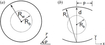
The geometries of the two systems are shown in figure 1, the system of interest here is figure 1(b), the radii of mirrors
 $R_{c}$
equals the distance
 $d$
in the confocal case. The grazing intersection between the dispersion of the cyclotron mode on the electron beam and a waveguide mode near the waveguide cutoff results in a high gain. The beam mode dispersion relation is given by
 $$\begin{eqnarray}\unicode[STIX]{x1D714}-s\unicode[STIX]{x1D6FA}_{0}/\unicode[STIX]{x1D6FE}-k_{z}v_{z}\cong 0\end{eqnarray}$$
and the waveguide mode dispersion relation is
 $$\begin{eqnarray}\unicode[STIX]{x1D714}^{2}/c^{2}-k_{t}^{2}-k_{z}^{2}=0,\end{eqnarray}$$
where
 $\unicode[STIX]{x1D714}$
is the frequency of the wave,
 $\unicode[STIX]{x1D6FA}_{0}=eB_{0}/m_{0}$
is the non-relativistic cyclotron frequency of the gyrating electrons,
 $e$
is the electronic charge,
 $B_{0}$
is the external magnetic field and
 $m_{0}$
is the rest mass of the electron.
 $\unicode[STIX]{x1D6FE}$
is the relativistic mass factor,
 $s$
is the cyclotron harmonic number,
 $v_{z}$
is the axial velocity of the electron,
 $c$
is the velocity of light and
 $k_{z}$
and
 $k_{t}$
are the longitudinal and transverse propagation constants, respectively.
(a) Cylindrical waveguide with radius of
 $R_{w}$
, (b) quasi-optical waveguide, with two mirrors with radius of curvature
 $R_{c}$
and separated by
 $d$
.
 $R_{b}$
is the radius of the electron beam and
 $p$
is the half-width of the mirror.

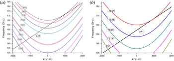
Dispersion relation for (a) cylindrical waveguide and (b) confocal waveguide with the
 $\text{TE}_{03}$
mode and
 $\text{TE}_{06}$
mode operating at the fundamental harmonic around 170 GHz, respectively.

For the
 $\text{TE}_{mn}$
mode in the cylindrical waveguide,
 $k_{t}=\unicode[STIX]{x1D707}_{mn}/R_{w}$
, where
 $\unicode[STIX]{x1D707}_{mn}$
is the
 $n$
th root of the derivation of the
 $m$
th-order Bessel function of the first kind
 $\text{J}_{m}^{\prime }(x)$
. For the confocal case, we define the half-width of the mirror as
 $p$
. For finite
 $p$
, taking the diffractive losses into consideration, then the full general equation of
 $k_{t}$
for the
 $\text{TE}_{mn}$
mode becomes
 $$\begin{eqnarray}k_{t}=(m/2+n+1/4)\unicode[STIX]{x03C0}/R_{c}+j\unicode[STIX]{x1D6EC}/2R_{c},\end{eqnarray}$$
where
 $\unicode[STIX]{x1D6EC}=2\ln [\sqrt{\unicode[STIX]{x03C0}}/R_{0,m}^{(1)}(C_{F},1)\sqrt{2C_{F}}]$
,
 $R_{0,m}^{(1)}$
is the radial wave function in prolate spherical coordinates.
 $C_{F}=kp^{2}/R_{c}$
is the Fresnel diffraction parameter and
 $k$
is the wavenumber in free space. Assuming the RF (radio frequency) fields are guided in the
 $z$
-direction, the loss rate in decibels per metre for the confocal waveguide of aperture
 $p$
can be written as
 $$\begin{eqnarray}\mathit{Loss~Rate}=-20\text{Im}\left.\left\{\sqrt{k^{2}-k_{t}^{2}}\right\}\right/\!\text{ln}\,10.\end{eqnarray}$$
In this paper, our discussion is limited to the lowest-order
 $m$
-modes. To simplify the loss calculation, a series of fits were performed and we have (Sirigiri et al.
Reference Sirigiri, Shapiro and Temkin2003)
 $$\begin{eqnarray}\left.\begin{array}{@{}c@{}}\log _{10}(\unicode[STIX]{x1D6EC})=-0.0069C_{F}^{2}-0.7088C_{F}+0.5443,\quad m=0\\ \log _{10}(\unicode[STIX]{x1D6EC})=-0.0226C_{F}^{2}-0.4439C_{F}+1.0820,\quad m=1\\ \log _{10}(\unicode[STIX]{x1D6EC})=-0.0363C_{F}^{2}-0.1517C_{F}+1.0075,\quad m=2.\end{array}\right\}\end{eqnarray}$$
The diffraction loss is an important factor for the confocal cavity. For the
 $\text{TE}_{mn}$
mode, the confocal waveguide effectively filters out modes with
 $m>0$
, as well as modes with lower
 $n$
(with a greater
 $C_{F}$
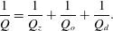
), and this is also the principle of mode selection. The dispersion relation is shown in figure 2 for the cylindrical and confocal waveguides. Owing to the diffraction loss, the mode density in the confocal case is greatly reduced. At the same time, it can be predicted that the quality factor will be lower than that of the cylindrical case due to the diffraction loss. Assuming a cavity guided in the
 $z$
-direction, in the cylindrical case, we have
 $$\begin{eqnarray}\frac{1}{Q}=\frac{1}{Q_{z}}+\frac{1}{Q_{o}},\end{eqnarray}$$
where
 $Q$
is the total quality factor,
 $Q_{z}$
and
 $Q_{o}$
are the quality factors related to the output power and Ohmic loss dissipated on the wall. In the confocal case, we have an additional diffraction loss, which is denoted by
 $Q_{d}$
in (2.7), so the total quality factor is lower than that in the cylindrical case
 $$\begin{eqnarray}\frac{1}{Q}=\frac{1}{Q_{z}}+\frac{1}{Q_{o}}+\frac{1}{Q_{d}}.\end{eqnarray}$$
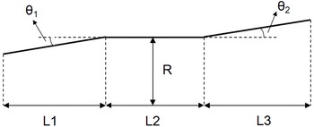
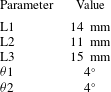
The resonator used in this paper is a three section smooth walled cavity structure as shown in figure 3. The input taper is a cutoff section which prevent the back propagation of RF power to the gun. The beam–wave interaction takes place mainly in the uniform middle section where the RF fields reach peak values. The uptaper connects the cavity with the output waveguide. The resonance frequency
 $\unicode[STIX]{x1D714}$
and quality factor
 $Q$
are determined by radiation boundary conditions at the resonator output section (Fliflet & Read Reference Fliflet and Read1981; Joye et al.
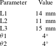
Reference Joye, Shapiro, Sirigiri and Temkin2009). The eigenmodes in the open-ended cavity resonator are obtained by solving the wave equation in the cavity geometry and applying radiation boundary conditions for minimum reflections to obtain resonant frequencies of the eigenmodes (Bernstein, Divringi & Smith Reference Bernstein, Divringi and Smith1982; Derfler, Grant & Stone Reference Derfler, Grant and Stone1982). In our analysis, the results are obtained with a beam voltage of 60 kV and a pitch factor of 1.3. The common parameters of the two cavities are listed in table 1. For the cylindrical cavity
 $R_{w}=2.86~\text{mm}$
and for the confocal cavity
 $R_{c}=5.525~\text{mm}$
,
 $p=2.3~\text{mm}$
.
Longitudinal section of the resonator.

Operating parameters of the cavity.
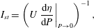
One of the most important problems in the design of high-power gyrotrons is to ensure that the device operates in the desired mode. Usually, single mode operation is desired and the starting current is an important parameter to analyse it. The starting current was defined as the minimum current for which
 $\text{d}P/\text{d}t>0$
in the limit
 $P\rightarrow 0$
: (Kreischer & Temkin Reference Kreischer and Temkin1980)
 $$\begin{eqnarray}I_{st}=\left(U\left.\frac{\text{d}\unicode[STIX]{x1D702}}{\text{d}P}\right|_{P\rightarrow 0}\right)^{-1},\end{eqnarray}$$
where
 $U$
is the beam voltage,
 $P$
is the output power and
 $\unicode[STIX]{x1D702}$
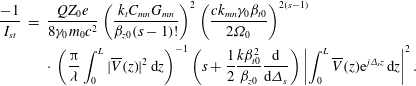
is the efficiency of beam–wave interaction. The starting current can be calculated by the linearized single mode theory (Borie & Jodicke Reference Borie and Jodicke1988; Nusinovich Reference Nusinovich1988)
 $$\begin{eqnarray}\displaystyle \frac{-1}{I_{st}} & = & \displaystyle \frac{QZ_{0}e}{8\unicode[STIX]{x1D6FE}_{0}m_{0}c^{2}}\left(\frac{k_{t}C_{mn}G_{mn}}{\unicode[STIX]{x1D6FD}_{z0}(s-1)!}\right)^{2}\left(\frac{ck_{mn}\unicode[STIX]{x1D6FE}_{0}\unicode[STIX]{x1D6FD}_{t0}}{2\unicode[STIX]{x1D6FA}_{0}}\right)^{2(s-1)}\nonumber\\ \displaystyle & & \displaystyle \cdot \,\left(\frac{\unicode[STIX]{x03C0}}{\unicode[STIX]{x1D706}}\int _{0}^{L}|\overline{V}(z)|^{2}\,\text{d}z\right)^{-1}\left(s+\frac{1}{2}\frac{k\unicode[STIX]{x1D6FD}_{t0}^{2}}{\unicode[STIX]{x1D6FD}_{z0}}\frac{\text{d}}{\text{d}\unicode[STIX]{x1D6E5}_{s}}\right)\left|\int _{0}^{L}\overline{V}(z)\text{e}^{j\unicode[STIX]{x1D6E5}_{s}z}\,\text{d}z\right|^{2}.\end{eqnarray}$$
The normalized profile of the electric field in the cavity is assumed to be Gaussian, that is to say,
 $\overline{V}(z)=\exp [-(2z/L-1)^{2}]$
. In (2.9),
 $L=L_{2}$
is the length of the uniform cavity.
 $C_{mn}$
is the normalization constant.
 $\unicode[STIX]{x1D706}$
,
 $Q$
and
 $Z_{0}$
are the wavelength in free space, quality factor and wave impedance, respectively.
 $\unicode[STIX]{x1D6FD}_{t0}=v_{t0}/c$
and
 $\unicode[STIX]{x1D6FD}_{z0}=v_{z0}/c$
are the initial transverse and longitudinal normalized velocity, respectively.
 $\unicode[STIX]{x1D6E5}_{s}=k(1-s\unicode[STIX]{x1D6FA}_{0}/\unicode[STIX]{x1D714}\unicode[STIX]{x1D6FE}_{0})/\unicode[STIX]{x1D6FD}_{z0}$
is the initial cyclotron resonance mismatch.
 $G_{mn}$
determines the beam–wave coupling and is defined as
 $$\begin{eqnarray}G_{mn}=\frac{1}{2\unicode[STIX]{x03C0}}\int _{0}^{2\unicode[STIX]{x03C0}}\left|\left(\frac{1}{k_{t}}\right)^{s}\left(\frac{\unicode[STIX]{x2202}}{\unicode[STIX]{x2202}x}+j\frac{\unicode[STIX]{x2202}}{\unicode[STIX]{x2202}y}\right)^{s}\unicode[STIX]{x1D6F1}(x,y)\right|^{2}\,\text{d}\unicode[STIX]{x1D711}\end{eqnarray}$$
in rectangular coordinates, and
 $$\begin{eqnarray}G_{mn}=\frac{1}{2\unicode[STIX]{x03C0}}\int _{0}^{2\unicode[STIX]{x03C0}}\left|\left(\frac{1}{k_{t}}\right)^{s}\left(\frac{\unicode[STIX]{x2202}}{\unicode[STIX]{x2202}r}+j\frac{1}{r}\frac{\unicode[STIX]{x2202}}{\unicode[STIX]{x2202}\unicode[STIX]{x1D711}}\right)^{s}\unicode[STIX]{x1D6F1}(r,\unicode[STIX]{x1D711})\right|^{2}\,\text{d}\unicode[STIX]{x1D711}\end{eqnarray}$$
in cylindrical coordinates.
In (2.10),
 $x=R_{b}\cdot \cos \unicode[STIX]{x1D711}$
,
 $y=R_{b}\cdot \sin \unicode[STIX]{x1D711}$
, where
 $R_{b}$
is the radius of the guiding centre. The membrane function of the
 $\text{TE}_{mn}$
mode for the cylindrical waveguide is
 $\unicode[STIX]{x1D6F1}(r,\unicode[STIX]{x1D711})=J_{m}(k_{t}r)\text{e}^{-jm\unicode[STIX]{x1D711}}$
. The membrane function of the
 $\text{TE}_{mn}$
mode for the confocal case is obtained by solving the paraxial wave equation (Joye et al.
Reference Joye, Shapiro, Sirigiri and Temkin2009).
 $$\begin{eqnarray}\unicode[STIX]{x1D6F1}(x,y)=\sqrt{\frac{R_{c}}{\sqrt{R_{c}^{2}+4y^{2}}}}H_{m}\left[\frac{2\sqrt{\unicode[STIX]{x1D712}}x}{\sqrt{R_{c}^{2}+4y^{2}}}\right]\exp \left[-\frac{\unicode[STIX]{x1D712}x^{2}}{R_{c}^{2}+4y^{2}}\right]\cdot \left\{\begin{array}{@{}l@{}}\cos \unicode[STIX]{x1D709},\quad n=2,4,6,\ldots \\ \sin \unicode[STIX]{x1D709},\quad n=1,3,5,\ldots ,\end{array}\right.\end{eqnarray}$$
where
 $\unicode[STIX]{x1D709}=-2\unicode[STIX]{x1D712}x^{2}y/R_{c}(R_{c}^{2}+4y^{2})+\unicode[STIX]{x1D712}/R_{c}y-1/2\arctan 2y/R_{c}$
,
 $\unicode[STIX]{x1D712}=\unicode[STIX]{x03C0}(n+m/2+1/4)$
and
 $H_{m}$
is the Hermite polynomial of order
 $m$
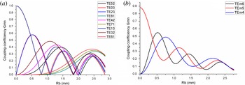
. The coupling efficiencies as a function of
 $R_{b}$
are shown in figure 4 for the cylindrical and confocal waveguides.
Distribution of coupling coefficients of the relevant modes at the fundamental harmonic for (a) the cylindrical gyrotron and (b) the confocal gyrotron.

3 Numerical results
Typically, the mode with the lowest power threshold will be excited first. As the beam parameters approach their final values, a different mode can be excited; thus, the starting current curves can provide useful information as to which mode is likely to be excited first (Borie & Jodicke Reference Borie and Jodicke1987; Kao et al. Reference Kao, Chiu, Pao and Chu2011).
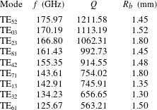
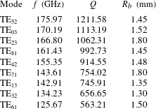
Eigenfrequencies
 $(f)$
and quality factors
 $(Q)$
of relative modes for the cylindrical cavity. The corresponding beam radius
 $R_{b}$
is also shown according to figure 5.
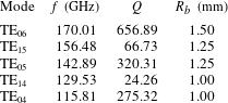
Eigenfrequencies
 $(f)$
and quality factors
 $(Q)$
of relative modes for the confocal cavity. The corresponding beam radius
 $R_{b}$
is selected according to figure 4.
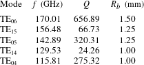
The eigenfrequencies and quality factors for relative modes together with the choices of beam radii for the cylindrical and confocal cavities are shown in tables 2 and 3, respectively. The radius of the guiding centre
 $R_{b}$
for each mode is carefully chosen in a reasonable region, such as to maximize the coupling of the electron beam to the RF field and to avoid coming too close to the wall of the cavity (Nusinovich Reference Nusinovich1981). The
 $\text{TE}_{03}$
mode in the cylindrical cavity corresponds to the
 $\text{TE}_{06}$
mode in the confocal cavity. As we have predicted, on the one hand, the quality factors of the confocal modes are generally lower than those of the cylindrical modes, on the other hand, owing to the diffraction loss in the confocal cavity, the
 $\text{TE}_{mn}$
modes with larger
 $m$
or lower
 $n$
in the confocal case have relatively lower
 $Q$
.
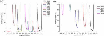
The starting current for the relative modes in cylindrical and confocal cavities have been plotted in figure 5. For the convenience of comparison, the start up situation is in the same region of magnetic field, namely
 $4.7\sim 7~\text{T}$
. So the competition mode
 $\text{TE}_{52}$
is taken into consideration. The starting current of the
 $\text{TE}_{02}$
mode is larger than 20 A and is not shown in figure 5(a). Results show that the mode density in the cylindrical cavity is very dense, hence another competition mode may easily oscillate when the beam current increases, although single mode operation is accessible in some specific region.
Starting currents for the relevant modes at the fundamental harmonic as a function of magnetic field in (a) the cylindrical cavity and (b) the confocal cavity, respectively.

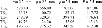
Quality factor
 $(Q)$
of relative modes for the confocal cavity with different
 $p$
.
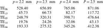
As to the confocal case, as shown in figure 5(b), the mode density seems to be regular and the curves have no intersection below 100 A. Firstly, the mode density is a constant as the modes with
 $m$
larger than 2 are ignored due to diffraction loss. Secondly, modes with larger
 $n$
have a lower starting current while modes with larger
 $m$
are much more difficult to oscillate. Thirdly, the starting current of the
 $\text{TE}_{06}$
mode keeps a certain distance away from the horizontal axis. That is to say, the confocal gyrotron is more qualified for operating as a high-value beam current and the confocal gyrotron is perhaps suitable for operating as a high-power gyrotron.
Two points have to be mentioned. Firstly, owing to the azimuthal symmetry of the cylindrical waveguide, the RF field is usually a linear combination of co-rotating and counter-rotating components. They have the same eigenfrequencies, so the mode density should be more intense. In this paper, only the co-rotating component is discussed in the cylindrical case, and the counter-rotating component is not plotted in figure 5(a) as its starting current is almost three to four times greater than that of the co-rotating component. However, this kind of problem does not exist in the confocal case. Secondly, the open sides of the confocal cavity not only filter out the unwanted modes, but also introduce an additional alterable parameter in the design. Table 4 shows the relation between the quality factor and some discrete
 $p$
. Results show that the quality factors increase as
 $p$
increases on account of a smaller diffraction loss. The good news is that the starting current is controllable through altering the mirror width. However,
 $p$
has a peak value as an overlarge
 $p$
will lead to a closed construction, where it is meaningless to discuss diffraction loss.
4 Summary
In this paper, based on linear theory, the mode density and starting current are researched for 170 GHz gyrotron with a traditional cylindrical cavity or a confocal cavity. The starting current is calculated for relative modes in the same region of the magnetic field. During this study, the beam radius is carefully chosen for each mode. Results show that the confocal gyrotron has a greater starting current and is capable of large-current operation.