2 Sagdeev pseudopotential formulation

We consider a general plasma fluid model consisting of an arbitrary number of species that may include any combination of dust, ion and electron species. The dynamics of inertial species are governed by the equations of continuity, momentum and pressure. The different species are coupled through Poisson’s equation, given in normalized variables by

where $\unicode[STIX]{x1D719}$ is the electrostatic potential, $x$ is the direction of the electrostatic plasma flow, $N$ is the number of species, and $n_{j}$ and $Z_{j}$ are the number density and charge of species $j$ , respectively. Here $Z_{j}>0\;(Z_{j}<0)$ corresponds to a positively (negatively) charged species.

The first step of a Sagdeev pseudopotential analysis (Sagdeev Reference Sagdeev and Leontovich1966) is to introduce a moving frame

This substitution simplifies the fluid equations to a system of ordinary differential equations. The densities of inertial species can then be solved by using the transformed equations of continuity, momentum and pressure. By substituting the transformed density equations into Poisson’s equation, and integrating, one obtains an energy-like integral of the form

Here the function $V(\unicode[STIX]{x1D719},M)$ is the Sagdeev potential.

Following Olivier et al. (Reference Olivier, Verheest and Maharaj2016), we introduce a Taylor series expansion of the Sagdeev potential $V$ about the equilibrium electrostatic potential $\unicode[STIX]{x1D719}=0$ and an acoustic speed $M=M_{0}$ . Here the acoustic speed $M_{0}$ satisfies the identity

In general, the Taylor series expansion can be written in the form

where

Here $\unicode[STIX]{x1D6FF}M$ is the incremental velocity satisfying $M=M_{0}+\unicode[STIX]{x1D6FF}M$ . It should be noted that the Sagdeev potential satisfies $V(0,M)=\unicode[STIX]{x2202}V/\unicode[STIX]{x2202}\unicode[STIX]{x1D719}(0,M)=0$ for all well-defined choices of $M$ . Therefore the coefficients $\unicode[STIX]{x1D70E}_{jk}=0$ for $k=0$ and $k=1$ , so that the second summation starts only at $k=2$ . For ease of presentation, we introduce the following notation:

Since we are interested in supersolitons of small amplitude, we consider the case where $|\unicode[STIX]{x1D719}|\ll 1$ . In this case, contributions of higher-order terms of $\unicode[STIX]{x1D719}$ are negligible, and may be ignored. For our analysis, we retain the first five orders of $\unicode[STIX]{x1D719}$ . The resulting approximation of the Sagdeev potential can then be written in the form

For the truncation (2.8) to be valid, $\unicode[STIX]{x1D719}$ must be sufficiently small so that contributions of the order $O(\unicode[STIX]{x1D719}^{6})$ (and higher) are negligibly small. In addition, we consider velocities that are only marginally faster than the acoustic speed, so that $\unicode[STIX]{x1D6FF}M\ll 1$ . We therefore only retain the lowest-order term of $\unicode[STIX]{x1D6FF}M$ for each order of $\unicode[STIX]{x1D719}$ in (2.8).

To start, we consider the lowest-order truncation for the coefficient $\unicode[STIX]{x1D719}^{2}$ in (2.8), given by

It is important to note that the left-hand side of (2.4) is $2B_{0}$ , so that $B_{0}=0$ . This means that the lowest-order term for the coefficient of $\unicode[STIX]{x1D719}^{2}$ in (2.8) is given by $B_{1}\unicode[STIX]{x1D6FF}M$ . Since we assume that $\unicode[STIX]{x1D6FF}M\ll 1$ , we neglect all higher-order terms of $\unicode[STIX]{x1D6FF}M$ , so that

For the third- to fifth-order terms of $\unicode[STIX]{x1D719}$ in (2.8), we consider only the case where the coefficients $C_{0}$ , $D_{0}$ and $E_{0}$ are non-zero. We can therefore make the following approximations:

By using the approximations (2.10) and (2.11), we can further truncate the series (2.8) to obtain the following approximation for the Sagdeev potential:

We assume that the Sagdeev potential $V(\unicode[STIX]{x1D719},M)$ satisfies the property

for $\unicode[STIX]{x1D719}\neq 0$ . This assumption follows from Verheest (Reference Verheest2010), who showed that this property holds for barotropic plasmas. By differentiating the Sagdeev potential (2.12), one obtains

From (2.13) and (2.14) it follows directly that

and throughout the paper we assume that $B_{1}<0$ .

It is important to mention some limitations of the approximation (2.12). We restrict this discussion to the subject of the paper, namely small-amplitude supersolitons. The amplitude of the supersoliton is given by a root of the Sagdeev potential. This root can be approximated from the cubic equation (2.12), and is denoted here by $\unicode[STIX]{x1D719}_{r}$ . Since the approximation is valid only for $|\unicode[STIX]{x1D719}|\ll 1$ , we naturally require that

In § 4 we show that the maximum supersoliton amplitude $\unicode[STIX]{x1D719}_{r}$ for a given plasma composition is directly proportional to the coefficients of the polynomial (2.12), so that

It is also shown that $\left|C_{0}\right|\propto D_{0}^{2}$ . Therefore, the requirement (2.16) implies that

A plasma composition where $C_{0}=D_{0}=0$ is called a supercritical composition (Verheest Reference Verheest2015; Verheest et al. Reference Verheest, Olivier and Hereman2016). We therefore refer to plasmas satisfying the criterion (2.18) as near-supercritical plasma compositions.

For all the terms in the approximation (2.12) to be significant, the contribution of the each term must be relevant near $\unicode[STIX]{x1D719}=\unicode[STIX]{x1D719}_{r}$ . Therefore the following relationship should be satisfied:

In addition, $|\unicode[STIX]{x1D719}_{r}|$ must be sufficiently small so that terms of order $O(\unicode[STIX]{x1D719}_{r}^{6})$ (and higher) are negligibly small.

One may use the relation (2.19) to approximate the velocities $\unicode[STIX]{x1D6FF}M$ of supersolitons. Indeed, from the relations (2.19) it follows that

so that

Therefore the restriction (2.16) ensures that $\unicode[STIX]{x1D6FF}M\ll |\unicode[STIX]{x1D719}_{r}^{3}|$ , so that the higher-order terms of $\unicode[STIX]{x1D6FF}M$ can be neglected. It should be noted that exact expressions for the supersoliton velocities are derived in § 4.

We briefly mention that the results derived can easily be extended to the case where $B_{1}=0$ . The lowest-order contribution of the coefficient of the $\unicode[STIX]{x1D719}^{2}$ term is then no longer $B_{1}\unicode[STIX]{x1D6FF}M$ , but becomes $B_{2}\unicode[STIX]{x1D6FF}M^{2}$ , so that the Sagdeev potential approximation becomes

While the results are similar, the only difference is that larger restrictions must be placed on the smallness of $\unicode[STIX]{x1D6FF}M$ to suppress higher-order contributions. Therefore the analysis of this paper can be extended to this special case. However, here we only consider the case where $B_{1}<0$ .

3 Supersolitons bounded by double layers

Double-layer solutions arise at a critical velocity in the form of a nontrivial root of the Sagdeev potential that is charge neutral. If the Sagdeev potential has an additional root beyond this point (in absolute terms), then supersolitons occur at velocities beyond this critical velocity. For such plasma compositions, the double-layer velocity acts as a lower limit of supersoliton velocities. In addition, the root beyond the double layer acts as a lower limit of the supersoliton amplitudes. We therefore start our analysis by considering plasma compositions that support both double layers and supersolitons.

Not all double-layer solutions give rise to supersolitons. It is important to emphasize that the converse also holds, namely that the existence of supersoliton solutions does not necessarily imply the existence of double-layer solutions. Such cases are dealt with in § 4.

Figure 1.

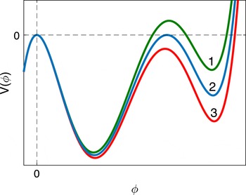
Generic illustration of Sagdeev potentials near double layers with additional roots. Curve 2 shows the Sagdeev potential at the critical velocity $M_{DL}$ where a double layer occurs. Beyond the double layer, the potential has an additional root. Curves 1 and 3 show Sagdeev potentials that arise slightly below and above the critical velocity $M_{DL}$ , respectively.

To obtain double-layer solutions that give rise to supersolitons, we look for plasma compositions that support Sagdeev potentials with three distinct nontrivial roots. This is due to the fact that three such roots can be found for Sagdeev potentials with velocities slightly below the critical double-layer velocity.

To illustrate this concept, consider figure 1, where a generic example of a Sagdeev potential with a root beyond the double layer is shown. Curve 2 (blue online) shows the Sagdeev potential at the critical velocity $M_{DL}$ where the double layer occurs. Beyond the double layer, there is an additional root that is not accessible from the origin. Curve 1 (green online) shows the Sagdeev potential at a velocity slightly smaller than $M_{DL}$ . It is clear that this curve has three nontrivial roots. Again, only the smallest root is accessible from the origin, giving rise to regular solitons. On the other hand, Curve 3 (red online) shows the Sagdeev potential at a velocity slightly larger than $M_{DL}$ . This potential corresponds to a supersoliton solution, as it has three charge-neutral points below the $\unicode[STIX]{x1D719}$ -axis. These charge-neutral points arise as the three turning points (local extrema) of the Sagdeev potential.

In the following, we provide a detailed analysis of obtaining three nontrivial roots for a Sagdeev potential of the form (2.12). The analysis developed here will also be applied in § 4, to find the general existence criteria for small-amplitude supersolitons.

To find nontrivial roots, we consider a Sagdeev potential of the form (2.12), which can be rewritten as

In terms of the roots, the factor $\unicode[STIX]{x1D719}^{2}$ simply gives rise to a trivial double root at the origin, corresponding to charge-neutrality at equilibrium. Therefore the nontrivial roots arise as roots of the cubic polynomial in the bracket,

The cubic polynomial (3.2) has at most three real roots. For these roots to give rise to supersolitons, we require that all three roots must be either positive (as in figure 1) or negative.

One may start the analysis by applying the classical Descartes’ rule of signs (Struik Reference Struik1986). In our context, this method allows us to determine the signs of the coefficients that are necessary to find either three positive or three negative real roots. For three positive roots, all the signs of the coefficients must alternate. Since $B_{1}<0$ , it follows that $C_{0}>0$ , $D_{0}<0$ and $E_{0}>0$ . On the other hand, for the possibility of three negative roots, all the signs of the coefficients must be the same. Since $B_{1}<0$ , it follows that all the coefficients must be negative.

These results can be summarized as follows. For the possibility of either three positive or three negative roots, we must have:

The polarity of the supersoliton is determined by the sign of the three roots. Since the condition $E_{0}>0$ ( $E_{0}<0$ ) gives rise to positive (negative) roots, it follows that the polarity of the supersolitons is positive when $E_{0}>0$ and negative when $E_{0}<0$ .

It is important to note that the condition derived above is necessary, but not sufficient for three roots. To find sufficient conditions, we analyse the roots of the cubic polynomial (3.2).

To analyse the roots of the cubic polynomial, we briefly review the roots of cubic equations. The solutions stated below are taken from Abramowitz & Stegun (Reference Abramowitz and Stegun1965).

Consider a general cubic equation

where $a_{0}$ , $a_{1}$ and $a_{2}$ are assumed to be real coefficients. The cubic equation (3.4) has three roots, given by

where

Cubic polynomials of the form (3.4) have at least one real root. The nature of the roots is determined by the sign of the discriminant $\unicode[STIX]{x1D6E5}$ . If $\unicode[STIX]{x1D6E5}>0$ , the cubic equation has one real root ( $z_{1}$ ) and two complex conjugate roots ( $z_{2}$ and $z_{3}$ ). If $\unicode[STIX]{x1D6E5}<0$ , the equation has three distinct real roots. If $\unicode[STIX]{x1D6E5}=0$ , the equation has a multiple root.

The polynomial (3.1) can be written in the form of (3.4) by setting

The discriminant $\unicode[STIX]{x1D6E5}$ of the polynomial $P_{1}$ is given by

The condition for three real roots is given by the inequality

To analyse the discriminant, we note that the factor in front of the bracket in (3.8) is always positive. Therefore the sign of the discriminant depends on the expression inside the brackets, given by

It should be noted that $\unicode[STIX]{x1D6FF}M$ is different from the other variables in the discriminant (3.8). While the other variables are determined by the plasma composition, the incremental velocity $\unicode[STIX]{x1D6FF}M$ is an independent variable in the sense that, for any given plasma composition, solitons can exist at many different velocities. This is analogous to linear theory where the wavenumber $k$ is treated as an independent variable. We can therefore treat the expression (3.10) as a quadratic function of the incremental velocity, given by

where

It is clear that this expression simply produces a parabola in the $\unicode[STIX]{x1D6FF}M$ – $\unicode[STIX]{x1D6E5}_{s}$ plane. Since $a>0$ , it follows that the parabola is concave upwards, so that it has a local minimum that also acts as the global minimum. Therefore, if the discriminant has negative values, it follows that the quadratic equation (3.11) has two distinct real roots. On the interval of $\unicode[STIX]{x1D6FF}M$ between these roots, the discriminant (3.8) is negative, meaning that the Sagdeev potential has three distinct real roots. We have therefore reduced the problem of finding plasma compositions that support both small-amplitude double layers and supersolitons to the analysis of the roots of the quadratic equation (3.11).

For real roots of (3.11), we must have

Substitution of the coefficients (3.12) into this existence criterion gives, after factorization:

For this criterion to be satisfied, the term inside the bracket must clearly be positive.

In the special case where the minimum value of the left-hand side of (3.14) is zero, the corresponding Sagdeev potential has a single nontrivial real root with multiplicity of three, i.e. a triple root. In this special case, a double-layer solution forms at a critical velocity. However, there are no roots beyond the double layer. Despite this, we show in § 4 that supersolitons still form at velocities beyond the double-layer velocity.

The condition (3.14) means that three nontrivial roots exist. However, to ensure that all three roots have the same sign, we also need to take the results from Descartes’ rule of signs (3.3) into account. By combining the criteria (3.3) and (3.14), we find the following criteria for obtaining three roots with the same sign:

When $E_{0}>0\;(E_{0}<0)$ the double layer has a positive (negative) polarity.

The roots of (3.11) give the range of incremental velocities where the discriminant (3.8) is negative. Therefore the Sagdeev potential (2.12) has three roots whenever

where

Here $\unicode[STIX]{x1D6FF}M_{1}$ and $\unicode[STIX]{x1D6FF}M_{2}$ correspond to the minus and plus signed solutions, respectively.

The double-layer solution arises at the critical velocity-increment

Therefore the double-layer velocity is given by $M_{DL}=M_{0}+\unicode[STIX]{x1D6FF}M_{DL}$ where $M_{0}$ is the appropriate acoustic speed. The velocity $M_{DL}$ also represents the lower limit of supersoliton velocities.

We can now determine the roots of the Sagdeev potential at the critical incremental velocity $\unicode[STIX]{x1D6FF}M_{DL}$ . To simplify the expressions of the roots, we note that the second condition in (3.15) can be written as follows:

where

From this notation, we write the coefficient $C_{0}$ as follows:

We can then rewrite the double-layer incremental velocity (3.18) as

where

The coefficient $\unicode[STIX]{x1D6FD}_{1}$ is a positive coefficient for $\unicode[STIX]{x1D6FC}$ on the interval (3.19).

We can now determine the roots of the Sagdeev potential at the critical double-layer velocity $M_{DL}$ by writing the polynomial (3.2) in the general form (3.4) with

From (3.5) one obtains the following roots:

where

The coefficient $\unicode[STIX]{x1D6FD}_{2}$ is a negative coefficient for $\unicode[STIX]{x1D6FC}$ on the interval (3.19).

From this, the double-layer amplitude can be expressed as

while the root beyond the double layer is given by

Note that both roots are directly proportional to $|D_{0}/E_{0}|$ .

It is important to emphasize that $\unicode[STIX]{x1D719}_{b}$ has no physical significance at the critical incremental velocity $\unicode[STIX]{x1D6FF}M=\unicode[STIX]{x1D6FF}M_{DL}$ , as the root is not accessible from the origin. However, it represents the lower limit (in absolute terms) of the supersoliton amplitudes. These supersolitons propagate with incremental velocities marginally larger than $\unicode[STIX]{x1D6FF}M_{DL}$ .

4 Supersoliton existence criteria for near-supercritical compositions

In the previous section, we obtained the existence criteria (3.15) for small-amplitude supersolitons that form beyond double-layer velocities. In such cases, we were able to identify the lower limit of the supersoliton velocities (3.18) and amplitudes (3.28). However, we were unable find the upper limits for supersoliton velocities and amplitudes. Moreover, supersolitons may exist in plasma compositions that support no double layers.

We have therefore adapted our analysis to find supersolitons directly. To accomplish this, we look for plasma compositions with Sagdeev potentials that have three charge-neutral points. All three charge-neutral points must be positive (negative) for positive (negative) polarity supersolitons. A charge-neutral point $\unicode[STIX]{x1D719}_{c}$ arises at a turning point in the Sagdeev potential satisfying $\unicode[STIX]{x2202}V/\unicode[STIX]{x2202}\unicode[STIX]{x1D719}=0$ and $V<0$ at $\unicode[STIX]{x1D719}=\unicode[STIX]{x1D719}_{c}$ .

For Sagdeev potentials of the form (2.12), charge-neutral points can be obtained by differentiating with respect to $\unicode[STIX]{x1D719}$ , giving rise to the polynomial

Clearly charge-neutral points will arise as the roots of this polynomial. The factor $\unicode[STIX]{x1D719}$ in front of the bracket simply corresponds to the charge-neutrality at equilibrium $\unicode[STIX]{x1D719}=0$ , while the nontrivial roots arise as the roots of the cubic polynomial in the bracket, given by

For supersolitons, we therefore require that the polynomial $P_{2}(\unicode[STIX]{x1D719})$ must have three distinct real roots with the same sign.

The analysis of this polynomial is identical to the one presented in § 3. We therefore skip over the details in deriving the existence criteria.

Firstly, the differentiation does not change the signs of the coefficients of the resulting polynomial (4.2). Therefore, the same existence conditions (3.3) obtained from Descartes’ rule of signs also limit the existence of three charge-neutral points with the same sign.

Secondly, the discriminant is given by

where

Once again, the sign of the discriminant is determined by the sign of $\unicode[STIX]{x1D6E5}_{s}$ , which can be written as a quadratic equation of $\unicode[STIX]{x1D6FF}M$ . After factorizing, it follows that the discriminant (4.3) is negative whenever

By combining the Descartes’ conditions (3.3) and the requirement that $\unicode[STIX]{x1D6E5}<0$ given by (4.5), one arrives at the following existence criteria for small-amplitude supersolitons:

A comparison between the criteria (3.15) and (4.6) shows that supersolitons form without double layers whenever

We can conclude that small-amplitude supersolitons may arise near supercritical plasma compositions. It should be noted, however, that supercritical compositions do not guarantee small-amplitude supersolitons, as there may exist supercritical compositions where no perturbation of compositional parameters can provide the necessary conditions for supersoliton existence, given by (4.6).

We can take the analysis a step further by establishing the velocities and amplitudes of supersolitons within the existence region. Two useful quantities are provided by the roots of (4.4), given by

On the interval $\unicode[STIX]{x1D6FF}M_{-}<\unicode[STIX]{x1D6FF}M<\unicode[STIX]{x1D6FF}M_{+}$ , one obtains three turning points satisfying $\unicode[STIX]{x2202}V/\unicode[STIX]{x2202}\unicode[STIX]{x1D719}=0$ . However, this does not ensure the existence of supersolitons. For example, although Curves 1 and 2 in figure 1 have three turning points, neither of them correspond to a supersoliton. Only Curve 3 corresponds to a supersoliton, since all three turning points lie below the $\unicode[STIX]{x1D719}$ -axis.

Since the roots of the Sagdeev potential is determined by a cubic polynomial, we can address this by simply requiring that the Sagdeev potential (2.12) must have only a single real root. For the lower limit, this can be realized by defining the minimum velocity as $M_{min}=M_{0}+\unicode[STIX]{x1D6FF}M_{min}$ , where

Here the first condition in the bracket is given by (3.15), corresponding to plasma compositions that support double layers. The second condition in the bracket is given by (4.7), corresponding to plasma compositions that do not support double layers.

From § 3 we know that three unique roots arise only at velocities below supersoliton velocities, so that the upper limit of supersoliton velocities is not interfered with by double layers. Therefore the upper limit of the supersoliton velocity is simply given by $M_{max}=M_{0}+\unicode[STIX]{x1D6FF}M_{max}$ , where

Combining these limits, it follows that supersolitons arise at incremental velocities

The amplitude of the supersoliton is given by the single real root of the Sagdeev potential (2.12). By factorizing the polynomial, the problem is reduced to finding the roots of the cubic polynomial $P_{1}$ , defined in (3.2), so that we look for the real root of the cubic equation

Since we are interested in the supersoliton amplitude, we can apply the existence criterion (4.6) to write the coefficient $C_{0}$ in the form

where the condition

must be satisfied to obtain small-amplitude supersolitons. Using this form, one can rewrite the critical incremental velocities (4.8) as

where

By substituting the expressions for $C_{0}$ and $\unicode[STIX]{x1D6FF}M_{\pm }$ into the coefficients of the polynomial (4.12), the real root is given by $z_{1}$ in (3.5). We therefore get

where

and $\unicode[STIX]{x1D6FE}_{1\pm }$ is given by (4.16).

From these expressions, one can find the minimum and maximum supersoliton amplitude (in absolute terms). The maximum amplitude is given by $\unicode[STIX]{x1D719}_{max}$ , where

When $0<\unicode[STIX]{x1D6FC}<1/3$ , the minimum amplitude is given by the root beyond the double layer (3.28). On the other hand, the minimum supersoliton amplitude is given by $\unicode[STIX]{x1D719}=\unicode[STIX]{x1D719}_{-}$ when $1/3\leqslant \unicode[STIX]{x1D6FC}<16/45$ .

These results can be summarized as follows: the supersoliton amplitude $\unicode[STIX]{x1D719}_{r}$ lies on the interval

where $\unicode[STIX]{x1D719}_{max}$ is given by (4.20) and $\unicode[STIX]{x1D719}_{min}$ is given by

Here $\unicode[STIX]{x1D719}_{b}$ and $\unicode[STIX]{x1D719}_{r-}$ are given by (3.28) and (4.17), respectively. We can therefore conclude that the supersoliton amplitude is directly proportional to $|D_{0}/E_{0}|$ . This implies that small-amplitude supersolitons arise near supercritical plasma compositions, as was discussed in § 2.

5 Case study: model with cold ions and two-temperature electrons

We present a case study that allows us to illustrate all the main features of the results obtained above. This is done by considering a well-studied plasma model consisting of a cold fluid ion species and a two-temperature Boltzmann electron species. We also use the model to compare the small-amplitude supersolitons with those obtained from the exact Sagdeev potential.

The normalized fluid equations are given by Verheest et al. (Reference Verheest, Olivier and Hereman2016):

In the fluid equations $n$ denotes the ion number density normalized with respect to the equilibrium ion density $N_{i}$ , while $v$ denotes the ion fluid velocity normalized with respect to the ion-acoustic speed $c_{ia}=\sqrt{K_{B}T_{\mathit{eff }}/m_{i}}$ with ion mass $m_{i}$ . Here $K_{B}$ denotes the Boltzmann constant and $T_{\mathit{eff}}=T_{c}/[f+(1-f)\unicode[STIX]{x1D70F}]$ denotes the effective temperature with electron temperature ratio $\unicode[STIX]{x1D70F}=T_{c}/T_{h}$ for cool (hot) electron temperature $T_{c}\;(T_{h})$ . The cool electron density $f$ is normalized with respect to $N_{i}$ . In addition, $\unicode[STIX]{x1D719}$ denotes the electrostatic potential normalized with respect to $K_{B}T_{\mathit{eff}}/e$ where $e$ is the electron charge, while

and

Finally, lengths $x$ and time $t$ are normalized with respect to the Debye length $\unicode[STIX]{x1D706}_{D}=\sqrt{\unicode[STIX]{x1D700}_{0}\unicode[STIX]{x1D705}T_{\mathit{eff }}/(N_{i}\text{e}^{2})}$ and the inverse plasma frequency $\unicode[STIX]{x1D714}_{pi}^{-1}=\sqrt{\unicode[STIX]{x1D700}_{0}m_{i}/N_{i}\text{e}^{2}}$ , respectively.

The Sagdeev potential can be obtained analytically, and is given by Baluku, Hellberg & Verheest (Reference Baluku, Hellberg and Verheest2010):

The acoustic speed $M_{0}$ satisfies (2.4). By differentiating the Sagdeev potential (5.6), one can easily show that the acoustic speed is given by

irrespective of the choice of compositional parameters $f$ and $\unicode[STIX]{x1D70F}$ .

One can also calculate the coefficients $B_{1}$ , $C_{0}$ , $D_{0}$ and $E_{0}$ by using the definitions (2.7). From the appropriate derivatives of the Sagdeev potential (5.6), it follows that

where $A_{n}=f\unicode[STIX]{x1D6FC}_{c}^{n}+(1-f)\unicode[STIX]{x1D6FC}_{h}^{n}$ .

In our analysis, we showed that small-amplitude supersolitons form near supercritical plasma compositions. Therefore, the first step in finding supersoliton solutions is to find a supercritical plasma composition.

Supercritical plasma compositions satisfy $C_{0}=D_{0}=0$ . From the relations (5.8), Baluku et al. (Reference Baluku, Hellberg and Verheest2010) showed that $C_{0}=0$ whenever

provided that $\unicode[STIX]{x1D70F}\leqslant 5-2\sqrt{6}$ . On the other hand, one can show from the definition (5.8) that compositions where $D_{0}=0$ satisfy the following cubic equation:

Figure 2.

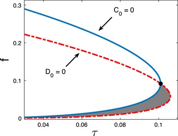
The boundaries where $C_{0}=0$ (solid line, blue online) and $D_{0}=0$ (dashed line, red online) are shown. The supercritical composition arises at the intersection of these boundaries, indicated by the dot (black online). In the shaded region, the necessary (not sufficient) condition (3.3) for small-amplitude supersolitons based on Descartes’ rule of signs is satisfied.

One can easily plot the curves where $C_{0}=0$ and $D_{0}=0$ in the $\unicode[STIX]{x1D70F}$ – $f$ plane. This is shown in figure 2. The solid line (blue online) shows the curve where $C_{0}=0$ , while the dashed line (red online) shows the curve where $D_{0}=0$ . We can see that these curves intersect, as indicated by the black dot. This intersection point is obviously a supercritical plasma composition, since $C_{0}=D_{0}=0$ . One may therefore look for supersolitons near this supercritical composition.

It should be noted that Verheest et al. (Reference Verheest, Olivier and Hereman2016) re-arranged the condition (5.10) in order to calculate the supercritical composition algebraically. They showed that the supercritical composition arises when $\unicode[STIX]{x1D70F}_{s}=5-2\sqrt{6}\approx 0.10102$ and $f_{s}=(3-\sqrt{6})/6\approx 0.0918$ .

At the supercritical composition, one finds that $E_{0}=1/5$ . Since $E_{0}>0$ , it follows that all small-amplitude supersolitons near the supercritical composition will have a positive polarity. The shaded region in figure 2 shows the region where the necessary (but not sufficient) condition for small-amplitude supersolitons (3.3) is satisfied, based on Descartes’ rule of signs. We can therefore narrow our search for small-amplitude supersolitons to this region of the compositional parameter space.

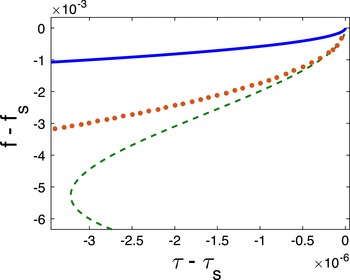
To find small-amplitude supersolitons, we need to find the region in the compositional parameter space that satisfies the existence criteria (4.6). The results are shown in figure 3. It should be noted that the axes are shifted in order to indicate the deviation from the supercritical composition, so that the origin represents the supercritical composition.

The solid line (blue online) in figure 3 shows the upper boundary where $C_{0}=0$ . The dashed line (green online) shows the boundary where $C_{0}E_{0}/D_{0}^{2}=16/45$ . The small-amplitude study predicts that supersolitons exist between these two lines. Interestingly, we see that the lower boundary turns away at $\unicode[STIX]{x1D70F}\approx \unicode[STIX]{x1D70F}_{s}-3.2\times 10^{-6}$ . Therefore, the small-amplitude study predicts no lower bound for the supersoliton existence region below this electron temperature ratio for the parameter range considered in figure 3.

Figure 3.

Existence region of supersolitons. The solid line (blue online) shows the upper boundary of supersolitons for both Sagdeev analysis and the small-amplitude study. The dashed line (green online) shows the approximation of the lower boundary via the small-amplitude study (4.6). The dots (red online) indicate the lower boundary as calculated from the Sagdeev analysis.

We also calculated the existence region of supersolitons using the exact Sagdeev potential (5.6). The lower boundary of the existence region is indicated with the dots (red online) in figure 3. In other words, supersolitons arise between the solid line and these dots. Since no approximations were necessary, this represents the correct existence region. We can clearly see that the results are similar for $\unicode[STIX]{x1D70F}-\unicode[STIX]{x1D70F}_{s}\geqslant -5\times 10^{-7}$ . However, for smaller values of $\unicode[STIX]{x1D70F}-\unicode[STIX]{x1D70F}_{s}$ , the results diverge. Indeed, we also see that the lower boundary obtained from the exact Sagdeev potential does not form a turning point as is observed for the small-amplitude study. We can therefore conclude that the small-amplitude study no longer applies in this region of parameter space. This divergence is due to a rapid growth of the supersoliton amplitude, associated with the approximation (2.21). As a result, higher-order contributions can no longer be ignored. This serves as a reminder that the small-amplitude study applies only to plasma compositions close to the supercritical composition.

It is interesting to take a closer look at the comparison between the small-amplitude approximation and the exact results obtained from the full Sagdeev potential (5.6). To do this, we fix the electron temperature $\unicode[STIX]{x1D70F}=\unicode[STIX]{x1D70F}_{s}-2\times 10^{-7}$ . In figure 3 we see good agreement of the existence regions of supersolitons between the small-amplitude theory and the exact results obtained via the Sagdeev potential. This implies that higher-order contributions are sufficiently small so that the truncated Sagdeev potential (2.12) with coefficients (5.8) provide a reasonable approximation for the Sagdeev potential (5.6).

We now compare the supersoliton amplitudes of the approximation with the exact values. This is done in figure 4. It is important to note that the values of $C_{0}$ , $D_{0}$ and $E_{0}$ depend on the cool electron density  $f$ .

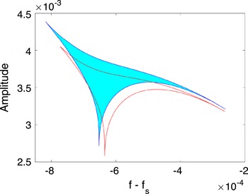
The shaded area (blue online) in figure 4 represents the supersoliton amplitudes as predicted by the small-amplitude approximation. At the density $f_{c1}$ where $f_{c1}-f_{s}\approx -6.52\times 10^{-4}$ , we see a sharp edge at the lower end of the existence region. This represents the critical density where $C_{0}E_{0}/D_{0}^{2}=1/3$ . At this density, the Sagdeev potential forms a triple root at the double-layer velocity $M_{DL}$ .

The critical density $f_{c1}$ separates the region where the small-amplitude theory predicts supersolitons bounded below by double layers $(f>f_{c1})$ or not $(f<f_{c1})$ . At this density, the small-amplitude theory predicts the widest range of possible supersoliton amplitudes and velocities.

Figure 4.

Comparison of supersoliton amplitudes for $\unicode[STIX]{x1D70F}=\unicode[STIX]{x1D70F}_{s}-2\times 10^{-7}$ . The filled region (blue online) shows the amplitudes as approximated from the small-amplitude study. The line (red online) shows the existence region as calculated from Sagdeev analysis.

In figure 4 we superimposed the existence region that was calculated via the Sagdeev potential, where no approximation was made. This is indicated by the curve (red online) situated slightly below the boundaries of the shaded region. Since no approximations were made in these calculations, they represent the exact solutions. It is clear that the approximate solution (shaded region) slightly overestimates the supersoliton amplitudes. Nevertheless, the results are in good agreement. It is also clear that the two sets of results share a similar shape, so that one may conclude that qualitative agreement is observed.

It is interesting to note that the exact solutions show a sharp point at a critical density $f_{c2}$ , where $f_{c2}-f_{s}\approx -6.343\times 10^{-4}$ , slightly larger than $f_{c1}$ . Numerical results show that this density represents the critical density where a triple root forms for the exact Sagdeev potential at its double-layer velocity. In addition, this density also separates the region where supersolitons are bounded below by double layers $(f>f_{c2})$ or not $(f<f_{c2})$ .

We conclude the case study by comparing the approximate Sagdeev potentials to the exact Sagdeev potentials. Keep in mind that the difference between these two sets of Sagdeev potentials is due to the truncation of higher-order terms in $\unicode[STIX]{x1D6FF}M$ and $\unicode[STIX]{x1D719}$ . To do this comparison, we once again fix $\unicode[STIX]{x1D70F}=\unicode[STIX]{x1D70F}_{s}-2\times 10^{-7}$ , and consider the two critical electron densities $f_{c1}$ and $f_{c2}$ .

Figure 5.

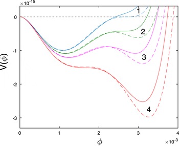
Sagdeev potentials for $\unicode[STIX]{x1D70F}=\unicode[STIX]{x1D70F}_{s}-2\times 10^{-7}$ and $f=f_{c1}$ at different velocities. The solid and dashed lines correspond to the exact Sagdeev potential and the approximate Sagdeev potential, respectively. Labels 1 (blue online), 2 (green online), 3 (magenta online) and 4 (red online) correspond to incremental velocities $\unicode[STIX]{x1D6FF}M\approx 3.9072\times 10^{-9}$ , $\unicode[STIX]{x1D6FF}M\approx 3.9792\times 10^{-9}$ , $\unicode[STIX]{x1D6FF}M\approx 4.062\times 10^{-9}$ and $\unicode[STIX]{x1D6FF}M\approx 4.2182\times 10^{-9}$ , respectively.

We first consider the critical density $f=f_{c1}$ , where $\unicode[STIX]{x1D6FC}=1/3$ , so that the approximate Sagdeev potential forms a triple root at the critical velocity $M=M_{DL}$ . As discussed above, the exact Sagdeev potential forms no double layer, since $f_{c1}<f_{c2}$ . The results are shown in figure 5. The labels 1–4 denote the different incremental velocities $\unicode[STIX]{x1D6FF}M\approx 3.9072\times 10^{-9}$ , $\unicode[STIX]{x1D6FF}M\approx 3.9792\times 10^{-9}$ , $\unicode[STIX]{x1D6FF}M\approx 4.062\times 10^{-9}$ and $\unicode[STIX]{x1D6FF}M\approx 4.2182\times 10^{-9}$ , respectively. For each label, the solid line corresponds to the exact Sagdeev potential, while the dashed line corresponds to the approximated Sagdeev potential.

For each label in figure 5, we see that the approximate Sagdeev potential (dashed lines) overestimates the root, i.e. the amplitude. Label 1 (blue online) corresponds to the critical incremental velocity $\unicode[STIX]{x1D6FF}M_{min}$ , representing the lower limit of supersoliton velocities. We see that the approximate Sagdeev potential (blue dashed line) forms a triple root (i.e. an inflection point on the $\unicode[STIX]{x1D719}$ -axis), giving rise to a double layer. On the other hand, the exact Sagdeev potential (blue solid line) has only a single root and a single charge-neutral point, meaning that a regular soliton would form at this velocity. Label 2 (green online) shows the Sagdeev potentials at the lower limit of supersoliton velocities for the exact Sagdeev potentials, corresponding to an inflection point. Since this inflection point is below the $\unicode[STIX]{x1D719}$ -axis, it follows that no double layers form. The dashed line shows that the approximate Sagdeev potential forms a local maximum below the $\unicode[STIX]{x1D719}$ -axis, thus predicting a supersoliton at this velocity. Label 3 (magenta online) shows the Sagdeev potentials at the incremental velocity $(\unicode[STIX]{x1D6FF}M_{min}+\unicode[STIX]{x1D6FF}M_{max})/2$ . Here we see that both the approximate and the exact Sagdeev potentials predict supersolitons. Label 4 (red online) shows the Sagdeev potentials at the incremental velocity $\unicode[STIX]{x1D6FF}M_{max}$ . The dashed line forms an inflection point, marking the upper limit of supersoliton velocities. We see good agreement between the approximate and the exact Sagdeev potential near the inflection point, so that the incremental velocity $\unicode[STIX]{x1D6FF}M_{max}$ is a good approximation of the upper incremental velocity of the exact Sagdeev potential. However, the roots are quite different, indicating that the approximate Sagdeev potential (dashed line) overestimates the upper limit of supersoliton amplitudes.

It is worth pointing out that the exact Sagdeev potentials (solid lines) in figure 5 are typical for supersolitons that form when no double layers exist. In this case, an inflection point forms below the $\unicode[STIX]{x1D719}$ -axis. This is clearly different to the case where double layers form, as illustrated in figure 1.

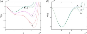
We now consider the critical density $f_{c2}$ where a triple root is found for the exact Sagdeev potential. Once again we used solid lines for the exact Sagdeev potential, and dashed lines for the approximate Sagdeev potentials. In figure 6(a) the labels 1 (blue online) and 2 (green online) correspond to the critical incremental velocity $\unicode[STIX]{x1D6FF}M_{min}\approx 3.4884\times 10^{-9}$ and $\unicode[STIX]{x1D6FF}M\approx 3.4959\times 10^{-9}$ , the latter being the lower limit of incremental velocities for supersolitons associated with the exact Sagdeev potential. These sets of results are difficult to distinguish on this scale, and are considered separately in part (b). Label 3 (magenta online) shows the Sagdeev potentials at the incremental velocity $(\unicode[STIX]{x1D6FF}M_{min}+\unicode[STIX]{x1D6FF}M_{max})/2\approx 3.6346\times 10^{-9}$ . Here we see that both the approximate and the exact Sagdeev potentials predict supersolitons. Label 4 (red online) shows the Sagdeev potentials at the incremental velocity $\unicode[STIX]{x1D6FF}M_{max}\approx 3.7808\times 10^{-9}$ . Once again we see good agreement between the approximate and the exact Sagdeev potential near the inflection point, so that the incremental velocity $\unicode[STIX]{x1D6FF}M_{max}$ is a good approximation of the upper incremental velocity of the exact Sagdeev potential.

In figure 6(b) we show only the Sagdeev potentials labelled 1 and 2. Curves i and iii (blue online) show the exact and approximate Sagdeev potentials at $\unicode[STIX]{x1D6FF}M_{min}$ , respectively. Here we see that the approximation predicts a double layer. However, the exact Sagdeev merely shows the existence of a regular soliton solution. Curves ii and iv (green online) show the exact and approximate Sagdeev potential at $\unicode[STIX]{x1D6FF}M\approx 3.4959\times 10^{-9}$ , respectively. At this velocity, Curve ii shows an inflection point on the $\unicode[STIX]{x1D719}$ -axis, i.e. a triple root. On the other hand, Curve iv shows that the approximate solution incorrectly predicts a supersoliton at this velocity.

Figure 6.

In (a), Sagdeev potentials for $\unicode[STIX]{x1D70F}=\unicode[STIX]{x1D70F}_{s}-2\times 10^{-7}$ and $f=f_{c2}$ at different velocities. The solid and dashed lines correspond to the exact Sagdeev potential and the approximate Sagdeev potential, respectively. In (a), labels 1 (blue online), 2 (green online), 3 (magenta online) and 4 (red online) correspond to incremental velocities $\unicode[STIX]{x1D6FF}M\approx 3.4884\times 10^{-9}$ , $\unicode[STIX]{x1D6FF}M\approx 3.4959\times 10^{-9}$ , $\unicode[STIX]{x1D6FF}M\approx 3.6346\times 10^{-9}$ and $\unicode[STIX]{x1D6FF}M\approx 3.7808\times 10^{-9}$ , respectively. In (b), only labels 1 and 2 are shown. Here Curves i and ii correspond to the exact Sagdeev potentials with the velocities of labels 1 and 2 above, respectively. Curves iii and iv show the approximate Sagdeev potentials with the velocities of labels 1 and 2, respectively.

The case study shows good agreement between the small-amplitude approximations and the exact Sagdeev potentials. We may therefore conclude that the small-amplitude theory is useful for obtaining regions in parameter space where small-amplitude supersolitons may occur. These solutions provide useful initial guesses for the existence regions of supersolitons. The full Sagdeev potential can then be used to obtain the exact results, especially for supersolitons with larger amplitudes.