
1. Introduction
Mechanical and biologic prostheses are routinely implanted as replacement for dysfunctional or diseased aortic valves. Isaacs et al. (Reference Isaacs, Shuhaiber, Salemi, Isom and Sedrakyan2015) reported that among the overall number of surgical replacement operations performed in the United States in the period 2007 to 2011, approximately 36.4 % of them were mechanical and 63.4 % were bioprosthetic. In the past decades the use of biologic prostheses increased substantially also due to the advent of transcatheter replacement technologies with self-expanding prostheses (Reardon et al. Reference Reardon2017), which are widely preferred for patients with severe aortic stenosis (Holmes et al. Reference Holmes2016). Despite such a continuously growing trend, the receipt of a biologic prosthesis was associated with a significantly higher 15-year mortality and a higher incidence of reoperation than the receipt of a mechanical prosthesis among patients 45 to 54 years of age (Goldstone et al. Reference Goldstone, Chiu, Baiocchi, Lingala, Patrick, Fischbein and Woo2017). Furthermore, the choice of the replacement procedure depends on patients’ comorbidities and concomitant artery diseases, which might affect the deployment phase in transcatheter replacement (Pai et al. Reference Pai, Kapoor, Bansal and Varadarajan2006). Thus, mechanical valves remain a clinically relevant option for cardiac surgery on patients with long life expectancy.
While bileaflet mechanical aortic valves (BMAVs) are more durable and resilient to tearing with respect to bioprosthetic valves, they nevertheless provide a non-physiological haemodynamics, which systematically entails high levels of fluid stress. Large haemodynamic stresses are known to be correlated to mechanical haemolysis, i.e. the lysis of red blood cells (RBCs), and platelets activation, which may initiate thrombosis (Bluestein, Rambod & Gharib Reference Bluestein, Rambod and Gharib2000). Hence, recipients of BMAVs need to be on a life-long anticoagulant therapy to prevent thromboembolic complications (Yoganathan, He & Casey Jones Reference Yoganathan, He and Casey Jones2004). According to statistics provided by Roudaut, Serri & Lafitte (Reference Roudaut, Serri and Lafitte2007), after ten years from the BMAV implantation, a range of  $10\,\%$ to
 $30\,\%$ dysfunctional valves was observed, detected by means of different events such as large pannus formation, increase of the pressure drop, abnormal leaflet kinematics and an increase of the regurgitation rate. The source of these complications has been clearly identified in the alteration of the physiologic flow topology, bringing larger stresses on the blood constituents (Yoganathan et al. Reference Yoganathan, He and Casey Jones2004), namely: (i) the three turbulent jets developed during the systolic phase instead of the single jet from the natural valve, (ii) the abrupt closing of the leaflets, (iii) the high shear flows within the hinges, and (iv) the large regurgitation flow rate.
In this scenario, direct numerical simulations (DNS) and fluid–structure interaction (FSI) approaches have helped shed light on the complex haemodynamics experienced downstream of BMAVs, providing a detailed three-dimensional description of the flow features. Most of the experimental facilities employed for the study of heart valve flows brought measurements with limited spatial resolution, whereas the energy cascade downstream of BMAVs are recognised to generate microscopic spatial scales. For instance, Yun et al. (Reference Yun, Dasi, Aidun and Yoganathan2014b) found a Kolmogorov length scale ranging from 80 to 45  $\mathrm {\mu }$m. Hence, numerical simulations represent the only viable tool for providing local quantitative predictions at the resolution required for the comprehension of the fluid-dynamic mechanisms behind thromboembolic complications (Sotiropoulos & Borazjani Reference Sotiropoulos and Borazjani2009). The present study is focused on the investigation of the general flow structure, with emphasis on turbulent features, past three different mechanical valve models, which are currently implanted or currently matter of research.
Despite clinical and experimental evidences showing that the turbulent stress level is highly correlated with cell damage, the fundamental relations linking different types of fluid stresses to RBC membrane failure remain unclear (Faghih & Sharp Reference Faghih and Sharp2019). In this connection, Reynolds stresses have often been employed as markers for the level of direct stress on blood constituents, although they do not physically act on the RBC membrane. Nevertheless, turbulent fluctuations can cause a local increase in the instantaneous viscous shear stress that the RBC might experience, as well as they can affect the dynamics of transport and collision of the blood suspended phase (Faghih & Sharp Reference Faghih and Sharp2019). Ellis, Wick & Yoganathan (Reference Ellis, Wick and Yoganathan1998) and Lu, Lai & Liu (Reference Lu, Lai and Liu2001) observed that the cell damage occurs as the Kolmogorov length scale (estimated by classic scaling laws) approaches the size of the RBCs; however, this trend provides no details on the damage mechanism, neither on the RBC interaction with dissipative scale eddies. On the contrary, Quinlan & Dooley (Reference Quinlan and Dooley2007) showed that shear is applied to cells in much larger eddies and may be more responsible for cell damage than Kolmogorov eddies. Antiga & Steinman (Reference Antiga and Steinman2009) suggested that blood constituents can act as a recipient of the energy carried by the smallest eddies, due to their high level of packing, which might be dissipated in viscous collisions. A reliable estimation of the blood damage across a mechanical aortic valve (MAV) must rely on a multiscale model, able to predict the stress distribution on blood elements in a Lagrangian sense, and to account for the exposure time to high shear and high vorticity regions. However, such a level of detail is computationally impractical for full-scale simulations of turbulent flow across mechanical valves. In view of these considerations, an accurate picture at several stages of the cardiac cycle of both viscous and turbulent stress distribution can provide globally meaningful estimations of relative risk to blood integrity. Beside the rupture of the RBC membrane, fluid stresses also cause platelet activation. Stress levels that are not considered harmful to RBCs can activate platelets and ultimately cause thrombosis (Sharp & Mohammad Reference Sharp and Mohammad1998), and the formed thrombus can in turn change the flow dynamics within the cardiovascular pathways and contribute to RBC damage (Faghih & Sharp Reference Faghih and Sharp2019). Hedayat, Asgharzadeh & Borazjani (Reference Hedayat, Asgharzadeh and Borazjani2017) recently compared the thrombogenic features of BMAVs and a bioprosthetic valves employing different models for platelet activation. They showed that the shear-induced platelet activation by mechanical valves is several folds larger than bioprosthetics at the end of the systole. Thus, the evaluation of the sublethal stress level is a key aspect of the flow field analyses. Further considerations on the effectiveness of Eulerian stress measures, and on the blood damage thresholds, are provided in the core of the manuscript.
Valve replacement by mechanical prostheses is commonly performed using bileaflet valves, offering decades of clinical experience in implantation methodology and post-operation scenarios. However, recent biomedical advances such as mechanical trileaflet valves and bileaflet valves with vortex generators (VGs) might potentially conjugate life-long durability with improved haemodynamic performance. The main goal of this study is to asses and compare the turbulent flow features of the aforementioned technologies to provide some landmarks for mechanical prostheses design and computational modelling.
With the objective of minimising the risk for platelet activation and haemolysis, previous studies utilised passive control flow surfaces such as VGs (Murphy et al. Reference Murphy, Dasi, Vukasinovic, Glezer and Yoganathan2010; Hatoum & Dasi Reference Hatoum and Dasi2019). Hatoum & Dasi (Reference Hatoum and Dasi2019) documented through in-vitro experiments that the use of VGs allows one to mitigate turbulent stresses and reduce the transvalvular pressure drop. Vortex generators for biomedical investigations appeared only in the aforementioned in-vitro investigations, whereas they have been extensively studied in aerospace applications as a mean to delay or even suppress flow separation by bringing momentum from the free stream into the boundary layer. In the context of confined flows with obstacles, such as those of BMAVs, VGs work on the basis of different principles. The presence of properly tilted obstacles on the downstream side of the valve leaflets was found to disperse and disintegrate the large-scale coherent structures shed from the leaflet edge in the systolic phase through additional instabilities. This results in a lower turbulent production (Hatoum & Dasi Reference Hatoum and Dasi2019), and consequently, a lower turbulent stress distribution. In this connection a computational investigation can provide further insights in this mechanism and overcome the practical limitations in the spatial and temporal resolution of a particle image velocimetry (PIV) apparatus and the two-dimensional nature of acquisitions.
The trileaflet design potentially provides a reduced thrombogenicity with respect to the bileaflet design because its haemodynamics in the systolic stage, governed by a central coherent jet, more closely resembles that of the native aortic valve. Several designs of this valve have been investigated over the years in-vitro (Linde et al. Reference Linde, Hamilton, Navalon, Schmitz-Rode and Steinseifer2012) and in-vivo (Gallegos et al. Reference Gallegos, Rivard, Suwan, Black, Bertog, Steinseifer, Armien, Lahti and Bianco2006) by animal trials. A recent study proved that trileaflet valves provide a more homogeneous core flow with lower global vorticity magnitude and reduced wall shear stress if compared with current bileaflet models (Li, Hegner & Bruecker Reference Li, Hegner and Bruecker2020) with similar implantation position. Furthermore, a comparative in-vitro study on leaflet kinematics (Carrel et al. Reference Carrel, Dembitsky, de Mol, Obrist, Dreyfus, Meuris, Vennemann, Lapeyre and Schaff2020) showed that recent trileaflet valves guarantee slower closing kinematics with respect to BMAVs, implying lower stress levels on blood flow. The present study provides a complementary description of the turbulent features within a recent trileaflet valve design, which corroborates the potential of trileaflet models in generating the more natural valve haemodynamics.
In the present manuscript we provide a thorough description of the procedures carried out to process the high-resolution simulation performed with particular focus on the collection of statistically meaningful average fields. The numerical approach, based on the immersed boundary (IB) method, is briefly described in the following section. Subsequently, a quantitative evaluation of a three-dimensional mean flow and turbulent stress field is presented. Then, relevant turbulent features are further explored by means of spectral analyses.
2. Methodology
2.1. Valve-aortic root model
In the present study the aortic root is configured as a rigid cylindrical channel of length  $L=5D$ separated in two branches with different diameters by three Valsalva sinuses. The upstream part of the channel has diameter
 $D$ and height
 $h_1=0.8D$, whereas the downstream part has diameter
 $1.16D$ and height
 $h_2=3.2D$. The reference length
 $D$ represents the annulus diameter, i.e. the inner diameter of the fibrous necking at the base of the aortic root. The size of the downstream channel and the geometry of the Valsalva sinuses (three identical elements with
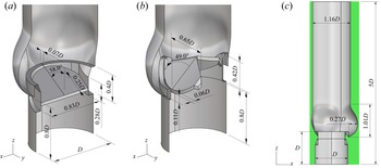
 $120^\circ$ symmetry) match the characteristic dimensions of a healthy specimen extracted by Reul et al. (Reference Reul, Vahlbruch, Giersiepen, Schmitz-Rode, Hirtz and Effert1990) from a cluster of angiographic films. A similar parametrisation procedure has been recently proposed by Xu et al. (Reference Xu, Morganti, Zakerzadeh, Kamensky, Auricchio, Reali, Hughes, Sacks and Hsu2018) to address the patient-specific design of bioprosthetic aortic valves. Further dimensions about the aortic root are reported in figure 1(a–c). In our model we do not distinguish coronary and non-coronary aortic sinuses. The upstream branch of the channel is configured in place of the left ventricular cavity to displace the leaflet leading edge from the inflow boundary condition, whereas the downstream channel substitutes the initial stretch of the ascending aorta. The length
 $h_2$ provides enough space to deplete the eddy turnover time within a cardiac cycle. Flow investigation downstream of
 $h_2$ has minimal practical interest, since the aortic root is bent immediately after the Valsalva sinuses. The length
 $h_1$ is chosen for minimal computational expense. Recent studies on biological (Lee et al. Reference Lee, Rygg, Kolahdouz, Rossi, Retta, Duraiswamy, Scotten, Craven and Griffith2020) and mechanical valves (Kim et al. Reference Kim, Choi, Kweon, Yang and Kim2020) with analogous discretization accuracy in space, have validated their simulations against experimental data using the same inlet-to-valve distance. Both velocity and pressure boundary conditions have shown to produce accurate results when setting the inlet-to-valve distance to 1D.
Cutaway view of three-dimensional model of the aortic root-housing-leaflets assembly with the principal measurements: (a) bileaflet mechanical valve, (b) trileaflet mechanical valve. (c) Front view of the valve-aortic root arrangement immersed in the computational domain (green area).

The valve models considered in the present study resemble the St Jude Medical Regent bileaflet valve (SJMV), whose patent is property of St Jude Medical Inc., Minnesota, USA, and the Lapeyre-Triflo FURTIVA mechanical heart valve (LTFV), whose patent is property of Novostia SA, Lausanne, Switzerland, both with annulus diameter  $D=23.0$ mm. The former has two planar, symmetric leaflets with straight cuts in correspondence of the pivot walls. The inner profile of the housing has two corresponding straight restrictions with two notches each receiving the leaflet hinges. In our model the hinge mechanism of the SJMV is not represented, the adequate solution of the flow field into the hinge interstices requiring a prohibitive computational expense. Such an issue has been addressed by means of a multiscale approach by Yun et al. (Reference Yun, Wu, Simon, Arjunon, Sotiropoulos, Aidun and Yoganathan2012). In place of the hinge mechanism, we introduce a small peripheral gap of width
 $0.007D$ to mimic the continuous washing through the effluent chimneys of the real mechanism. Eventually, the valve orientation follows the criterium of minimal turbulence production prescribed by Kleine et al. (Reference Kleine, Perthel, Nygaard, Hansen, Paulsen, Riis and Laas1998), with the leaflet symmetry axis bisecting one sinus (visible in figure 4). The clinical experience suggests that the valve orientation greatly affects several haemodynamic features such as the coronary flow rate and the leaflet dynamics (Haya & Tavoularis Reference Haya and Tavoularis2016). However, it is known that the choice of the valve orientation is subjected to the patient-specific surgical implantation procedure and to the surgeon's judgement. In this scenario, the minimal turbulence criterion matches the purposes of this study. The rotation arc of each leaflet during the motion is fixed to
 $55^\circ$. It is worth noting that in practice each leaflet rests in the diastolic phase at an angle of
 $60^\circ$ with respect to the streamwise direction (fully closed position) and opens up to an angle of
 $5^\circ$ (fully open position). In our numerical simulations the actual fully closed position is limited to an angle of
 $58^\circ$ to avoid the full leaflet-leaflet and leaflet-housing contact during the diastolic phase, preventing extreme backflow accelerations at valve closure. Further geometric details of the SJMV model can be inferred from figures 1(a) and 2(a).
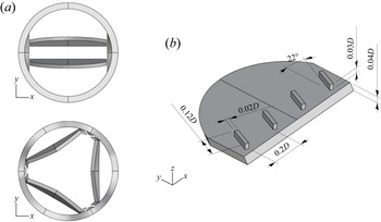
(a) Top view of the housing-leaflets assembly with the leaflet in the fully open configuration. (b) Isometric view of a leaflet with the VGs arrangement considered in this study.

The LTFV prosthesis provides three slightly curved leaflets with  $120^\circ$ symmetry, which allow us to replicate the haemodynamic pattern of a native biological valve with a large central orifice in the fully open configuration. Several versions of this valve have been studied over the years in-vitro (Ghista Reference Ghista1976), and its in-vivo performance are a current matter of interest. Each model leaflet has width
 $L_w=0.65D$, and radius of curvature in the cross-flow direction
 $r=30D$. Unlike the SJMV model, the hinge mechanism is represented by means of a simple trapezoidal appendage of the leaflet and a cylindrical plugin of the valve housing (the reader should refer to figure 2a), resembling the leaflet ear and the flange. These details are included in the model because they constitute an additional obstruction within the valve lumen, affecting the efflux haemodynamics (Vennemann et al. Reference Vennemann, Rösgen, Heinisch and Obrist2018), differently from the SJMV configuration. The valve orientation follows the aortic root arrangement, with each leaflet projected onto one aortic sinus. The rotation arc of each leaflet during the motion is fixed to
 $50^\circ$. Hence, each leaflet rests in the diastolic phase at an angle of
 $55^\circ$ with respect to the streamwise direction (fully closed position) and opens up to an angle of
 $5^\circ$ (fully open position). However, similarly to the SJMV, the actual closing angle is limited to
 $53^\circ$.
It is worth pointing out that in our model the relative position of both bileaflet and trileaflet valves with respect to the aortic root replicates the supra-annular configuration, meaning that the valve ring is placed above the tissue annulus, and the leaflets extend into the Valsalva sinuses. This is the most widespread implantation layout, since it was found to provide superior haemodynamic performance, dictated by clinical indicators (Kim et al. Reference Kim, Kim, Kim, Jung, Choo, Chung and Lee2019). The cuff sewing ring is not modelled, therefore, the aortic wall is in contact with the outer housing ring (the reader should refer to figure 1(a) for ease of comprehension). Both valve models have an identical inner housing diameter, corresponding to  $D_i=0.94D$, i.e.
 $21.5$ mm, and identical leaflet thickness, equal to
 $0.9$ mm.
In this study we also consider a SJMV model with a row of VGs per leaflet, installed on the aortic side, in proximity of the leading edge. The application of VGs to MAVs was first proposed by Murphy et al. (Reference Murphy, Dasi, Vukasinovic, Glezer and Yoganathan2010) and Hatoum & Dasi (Reference Hatoum and Dasi2019) with the common intent of reducing the shear stress level on blood constituents, both in the regurgitation phase and at systolic peak flow rate. When focusing on the latter condition, different VG configurations have been tested, with the lowest turbulent shear stress level associated to the ‘co-rotating’ arrangements (Hatoum & Dasi Reference Hatoum and Dasi2019). Therefore, we investigate precisely the co-rotating arrangement, made by four parallel VGs tilted by  $22^{\circ }$. The VG height is chosen to be
 $0.03D$, length
 $0.12D$, thickness
 $0.02D$ and spacing
 $0.2D$, based on the design indications proposed by Hatoum & Dasi (Reference Hatoum and Dasi2019). In aeronautical applications similar appendages have been miniaturised down to
 $0.3\div 0.5$ times the boundary layer thickness to maximise the boundary layer energising effect with minimal drag penalty. In these applications the boundary layer is modulated by the lift-up mechanism triggered by contro-rotating vortices observed experimentally (Fransson & Talamelli Reference Fransson and Talamelli2012) and numerically (Siconolfi, Camarri & Fransson Reference Siconolfi, Camarri and Fransson2015). In view of the complexity of BMAV flows, the VGs are simply expected to generate a contra-rotating structure corrupting the large-scale vortices shed from the leaflet trailing edge, which trigger the turbulent transition. Thus, as a matter of principle, the VGs height and angle should introduce the desired instability effects with limited penalty drag and orifice area reduction.
2.2. Numerical set-up
Direct numerical simulations are carried out by solving the Navier–Stokes equations for incompressible flows,
 \begin{equation} \left.\begin{gathered}
\frac{\partial u_i^*}{\partial t^*}+\frac{\partial u_i^*
u_j^*}{\partial x_j^*} ={-}\frac{\partial p^*}{\partial
x_i^*}+\frac{1}{{Re}} \frac{\partial^2 u_i^*}{\partial
(x_i^* )^2} +f_i^{*}, \\ \frac{\partial
u_i^{*}}{\partial x_j^{*}} = 0, \end{gathered} \right\}
\end{equation}
where the non-dimensional  $(\cdot )^*$ quantities
 $u_i^*$,
 $p^*$ and
 $f_i^*$ denote the flow velocity components, the pressure and the IB-volume force, respectively;
 $t^*$ indicates the time variable and
 ${Re}=U D/\nu$ is the Reynolds number, defined by the peak bulk velocity, annulus diameter and blood kinematic viscosity. Unless otherwise stated, data presented in this study are non-dimensionalised by the following characteristic parameters: velocity scale
 $U$ equal to the bulk velocity at the peak flow rate, length scale
 $D$ equal to the annulus diameter, time scale
 $D/U$ and pressure/stress scale
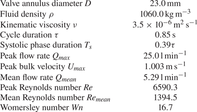
 $\rho U^2$. The scaling factors are summarised in table 1.
Fundamental parameters of the considered cardiac cycle.

Following a well-established assumption, blood is modelled as a Newtonian fluid (Caballero & Laín Reference Caballero and Laín2013). Under the operating physiological conditions of large blood vessels, the deviation from linearity in the viscosity-shear rate relation can be considered negligible (Siginer, De Kee & Chhabra Reference Siginer, De Kee and Chhabra1999; Vlachopoulos, O'Rourke & Nichols Reference Vlachopoulos, O'Rourke and Nichols2011) at the macroscopic spatial scale. Despite such rheologic evidences, recent numerical investigations (De Vita, de Tullio & Verzicco Reference De Vita, de Tullio and Verzicco2016; Ghigo, Lagrée & Fullana Reference Ghigo, Lagrée and Fullana2018) have shown that localised regions of high shear generated downstream of a BMAV provides prominent non-Newtonian effects. However, the uncertainty in the parameters of available constitutive models (Yilmaz & Gundogdu Reference Yilmaz and Gundogdu2008) and the complexity of the viscoelastic behaviour of the RBCs membrane, make the choice of non-Newtonian models unnecessary in the present work. Thus, we consider a constant viscosity of  $3.5 \times 10^{-6}\,\textrm {m}^2\,\textrm {s}^{-1}$, equal to the blood viscosity in the ascending aorta at the largest shear rate.
The cardiac cycle duration is set to  $\tau =0.85$ s, corresponding to about
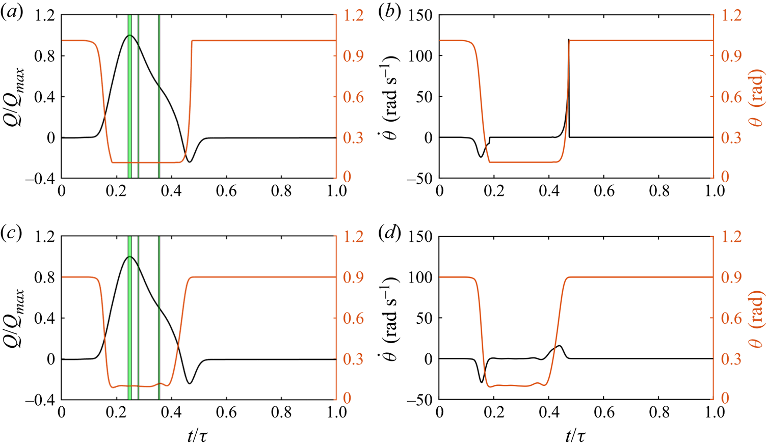
 $70$ beats min−1. In this work the inflow rate is prescribed at the inlet surface following the time law depicted in figure 3(a) for all simulations, where the apical flow rate
 $Q_{{max}}=25$ l min
 $^{-1}$ is reached at approximately
 $0.21$ s. This curve, together with the considered annulus diameter (
 $D=23$ mm), entails a mean flow rate equal to
 $Q_{{mean}}=5.29$ min−1. The listed parameters yield a peak Reynolds number equal to
 $6590$. A maximum negative flow rate
 $Q=-0.24 Q_{{max}}$ is provided at the leaflet closing to reproduce the reverse flow condition owing to the adverse pressure gradient generated from the ventricle expansion. A plug flow profile is prescribed owing to the high Womersley number (
 $Wn=16.7$) in this configuration. We emphasise that the inflow rate profile, plotted in figure 3, resembles the curve obtained in Lee et al. (Reference Lee, Rygg, Kolahdouz, Rossi, Retta, Duraiswamy, Scotten, Craven and Griffith2020) coupling an FSI solver with a three-element Windkessel model providing the driving boundary conditions through a bovine pericardial valve. The fundamental physical parameters of the cardiac cycle are summarised in table 1.
Time traces of the leaflet angular position superposed with the prescribed flow rate (a–c), and leaflet angular velocity (b–d). Plots (a,b) refer to the SJMV model, whereas plots (c,d) refer to the LTFV model.

The incompressible Navier–Stokes equations are discretised in space using second-order-accurate central differences on a staggered Cartesian grid. Such an approximation of spatial derivatives does preserve kinetic energy and circulation in absence of time-differencing errors and viscosity (Moin & Verzicco Reference Moin and Verzicco2016), providing an effective tool for the resolution of separated flow regions and complex vortex dynamics at moderate Reynolds numbers (Orlandi Reference Orlandi2012). The system (2.1) is solved by the conventional fractional step scheme (Moin & Kim Reference Moin and Kim1982). The provisional field is obtained by an approximate factorisation of the Helmholtz equation, whereas the Poisson equation is solved by a direct method. The momentum equation is advanced in time by means of a semi-implicit scheme, where the viscous terms are resolved with an implicit Crank–Nicolson method and the convective terms are discretised by an explicit Adams–Bashforth scheme.
The interface conditions are enforced through the IB method (Mittal & Iaccarino Reference Mittal and Iaccarino2005). The IB method provides the most convenient approach for dynamic MAV simulations with respect to body-fitted methods, since the large angular excursion of the leaflets would entail unpractical changes in the grid topology for body-fitted methods. Furthermore, when demanding remeshing procedures and field-variable interpolations are required, sophisticated algorithms must be employed to achieve a well-conditioned grid and limited artificial diffusivity with a reasonable computational effort (Tezduyar & Sathe Reference Tezduyar and Sathe2007). In the present work a Lagrangian-forcing with a moving least square (MLS) interpolation/spreading procedure is employed. The surface is identified in the flow field by a cluster of Lagrangian markers (Uhlmann Reference Uhlmann2005), at which the flow variables are interpolated by a MLS algorithm (Vanella & Balaras Reference Vanella and Balaras2009) with minimal oscillations in time. At each marker we compute a volume force from the difference between body velocity and interpolated velocity to obtain the equivalent force needed to match the no-slip condition locally. In the second instance the volume force is spread back to the Eulerian field and inserted into the momentum equation (2.1) to account for the interface condition. The numerical scheme and the IB procedure are thoroughly described and explored in the context of a fluid–structure-interaction solver in Nitti et al. (Reference Nitti, Kiendl, Reali and de Tullio2020) and de Tullio & Pascazio (Reference de Tullio and Pascazio2016). In the present simulations the local relative spacing among Lagrangian markers is set to  $0.6 \Delta x$, following the numerical experiments presented in Nitti et al. (Reference Nitti, Kiendl, Reali and de Tullio2020). According to the geometric arrangement illustrated in figure 1(c), the fluid domain which contains the aortic root has inflow–outflow conditions in the streamwise direction. At the inflow surface a velocity profile is assigned by a hyperbolic tangent function which yields a flat velocity distribution in the bulk and accommodates the no-slip boundary condition at the aortic wall within a layer of thickness
 $\lambda /D = 1/\sqrt {{Re}} \approx 1.22 \times 10^{-2}$. Such an inflow profile, in cylindrical coordinates takes the form
 \begin{equation} u^*(r^*)=\tanh (\frac{D}{4 \lambda} \left(1 - 2r^*)\right), \end{equation}
 $r^*$ being the radial coordinate. At the outflow boundary the non-reflecting condition proposed by Jin & Braza (Reference Jin and Braza1993) is implemented. It consists of resolving a diffusion–convection equation on the outlet face which minimises the feedback noises and correctly predicts the turbulent dynamics of the flow near the boundary, with greater effectiveness of the simpler radiative outlet condition (Orlanski Reference Orlanski1976). This condition was widely employed in turbulent flow analyses (Persillon & Braza Reference Persillon and Braza1998; Pier Reference Pier2002), and allows us to reduce the length of the computational domain and exploit the rear domain part for flow investigations. The following condition is resolved at the outlet face:
 \begin{equation} \frac{\partial u^*_i}{\partial t^*}+w^*\frac{\partial u^*_i}{\partial z^*}- \frac{1}{{Re}} \left(\frac{\partial^2 u_i^*}{\partial (x^*)^2} + \frac{\partial^2 u_i^*}{\partial (y^*)^2} \right) = 0. \end{equation}
This is resolved with the same temporal discretisation of the Navier–Stokes solver; therefore, it requires the solution of a linear system at the boundary nodes, which is performed by an approximate factorisation for efficiency purposes.
The present simulations are performed imposing the kinematics of the leaflets together with the inflow profile, based on previous fully coupled, FSI simulations (see figure 3), on the same configurations. A detailed discussion about the preliminary FSI investigation is provided in Appendix A. This choice was motivated by the necessity of reducing the computational expense. Furthermore, it allows us to reduce the level of uncertainty of statistical measurement by removing cycle-to-cycle variations of the leaflet dynamics, which can result in artificially high estimates of the turbulent features of the pulsatile flow (Tiederman, Privette & Phillips Reference Tiederman, Privette and Phillips1988).
The aortic root model is immersed in a computational domain of size  $1.5D \times 1.54D \times 5D$ (the reader should refer to the green box in figure 1c), uniformly discretised in the
 $X$,
 $Y$ and
 $Z$ directions by
 $421 \times 431 \times 1401$ grid points, resulting in a mesh with more than 250 million nodes, and minimum grid spacing equal to
 $3.56 \times 10^{-3} D$. In terms of physical resolution, this spacing corresponds to
 $82.0\,\mathrm {\mu }$m, which closely matches the minimum Kolmogorov length scale
 $\eta =40\,\mathrm {\mu }$m observed within the cardiac cycle by DNS performed with similar spatial resolution and scheme accuracy (Yun et al. Reference Yun, Dasi, Aidun and Yoganathan2014b). Although the resolution might be insufficient to resolve the smallest dissipative scale structures, the numerical simulations keeping this Kolmogorov scale-resolution ratio are still able to resolve the lower-order moments of the turbulent flow (Yeung & Pope Reference Yeung and Pope1989; Pope Reference Pope2001). Eventually, this grid has been subjected to an extensive grid refinement study (see Appendix B). All the simulations have been run at a fixed Courant–Friedrichs–Lewy (CFL) number, namely
 $\textrm {CFL}= (u_i^* )_{{max}} \Delta t^*/\Delta x^* =0.2$, adjusting the time step size accordingly. This procedure greatly enhances the computational efficiency of the time integration, since the systolic phase, which entails the largest local velocity peaks, occupies less than half the cardiac cycle (see figure 3). During most of the diastolic phase the mean velocity field is almost null everywhere, thus, the fluid equations can be integrated with much larger time steps. A minimum time step size of
 $\Delta t \approx 1.1 \times 10^{-4} U/D$ is achieved in the closing stage of the SJMV valve, when the largest leaflet acceleration is reached.
2.3. Collection of statistics
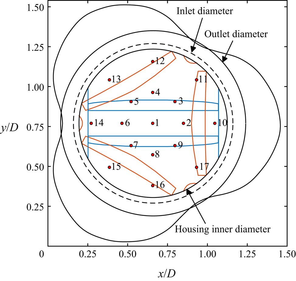
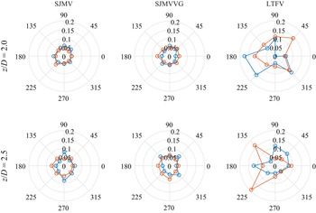
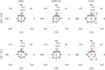
Although the flow through a straight aortic root resembles the standard turbulent pipe flow, the pulsatile nature of the inflow condition and the presence of the leaflets-housing assembly make the flow field inhomogeneous and anisotropic (Andersson & Karlsson Reference Andersson and Karlsson2021). Even in classic turbulent pipe flow the transverse velocity fields are considered not to satisfy the homogeneity condition (Kim, Moin & Moser Reference Kim, Moin and Moser1987), owing to the interaction with the walls. The streamwise velocity component and the associated energy are considered the most appropriate for the assumption of homogeneity. In this connection, beside classical turbulence stress analyses, we propose a local analysis of turbulence correlations and spectra. In particular we sample the velocity components on different monitor lines aligned with the aortic axis, inspecting different positions of the vessel's cross-sectional area, as depicted in figure 4.3 The monitor lines start downstream of the leaflets in the fully open position and run up to the outflow section. Thus, velocity components are collected within each time interval  $T_n$ over seventeen sampling lines, which are located at the aortic centreline (corresponding to the valve axis), at radial positions equal to
 $1/3$ and
 $2/3$ of the outlet root diameter, with uniform azimuthal distribution. One can notice from figure 4 that the inner line annulus is placed in correspondence of the SJMV leaflets in the fully open position, whereas they do not overlap with the LTFV leaflet shape.
Schematic top view with enumeration of the monitor lines used for the computation of the local correlations. Black lines represent the shared edges of the geometry, whereas the blue lines and the orange lines represent the footprint of the SJMV model and of the LTFV model, respectively, with the leaflets in the fully open configuration.

Within each cycle-resolved analysis, three cycle-averaged instants of interest are investigated to asses the relevant features of the flow field. These are identified in time as a function of the prescribed inflow rate law: peak flow rate (PF) at  $t_1=0.248 \tau$, early deceleration (ED) at
 $t_2=0.279 \tau$, late deceleration (LD) at
 $t_3=0.354 \tau$. The corresponding instantaneous flow rates are
 $Q/Q_{{max}}=[1.0,0.9,0.5]$, respectively. The acceleration phase is excluded from this comparative study about turbulent flow features since the flow is essentially laminar in this phase, with the residual vortical structures being washed out by the incoming flow. It is also important to stress that in the adopted numerical approach the pressure is defined only at the interior part of the computational domain and no pressure boundary conditions can be set. A limitation of this approach is that prescribing the flow rate as a boundary condition makes it impossible to impose a realistic pressure difference across the valve during the diastolic phase of the cycle. Thus, with the present arrangement, the leaflet closure is driven by a prescribed reverse flow rate (see figure 3a), that is the same for all the considered valve models, rather than a pressure gradient. Although the leaflet kinematics obtained with the present method closely resembles that observed in mock loop experiments (Vennemann et al. Reference Vennemann, Rösgen, Heinisch and Obrist2018), any speculation about the closing dynamics and related stresses would be inappropriate. Hence, our study focuses on the stresses in the systolic phase of the cycle. In this connection, assuming that the low-frequency mean velocity field and the high-frequency turbulence fluctuation are not correlated in the time and frequency domains, phase-averaged statistical data are collected over
 $N$ cardiac cycles, with
 $N=18$. However, in the context of a pulsatile, fully turbulent flow a huge amount of cycles would be needed to collect a statistically meaningful amount of samples, resulting in a computationally prohibitive task. To circumvent this issue, we collect the mean field of the generic variable
 $\phi$ within the time interval
 $T_n$ centred in the time instant
 $t_n$, for each cycle instant of interest
 $n$, i.e.
 \begin{equation} \bar{\phi}(\boldsymbol{x},t_n)= \frac{1}{N} \sum_{k=1}^{N} \left( \frac{1}{T_n} \int_{t_n-T_n/2}^{t_n+T_n/2} \phi(\boldsymbol{x},t)\,{\rm d} t\right). \end{equation}
Thus, each phase-averaged quantity is computed by an ensemble average over  $N$ time-averaged fields. Such a technique has already been employed in the study of flow fields through MAVs in experimental (Liu, Lu & Chu Reference Liu, Lu and Chu2000; Haya & Tavoularis Reference Haya and Tavoularis2016) and computational works (Yun et al. Reference Yun, Dasi, Aidun and Yoganathan2014a). It is worth noting that the duration of the time segment
 $T_n$ should be long enough to provide statistical validity of the results, but, at the same time, short enough to consider the flow field statistically steady within the time window. In this respect, we defined the width of each sampling window
 $T_n$ as the time interval in which a flow rate variation of
 ${\pm }1.0\,\%$ occurs. These intervals are highlighted by green stripes in figure 3(a–c). The described procedure leads to the collection of acceptable first- and second-order statistical fields. Further details about the sampling of statistically relevant quantities are reported in Appendix C.
Provided the definition of the mean (phase-averaged) field in (2.4), the instantaneous fluctuation is accordingly defined as
 \begin{equation} \phi'(\boldsymbol{x},t_n)=\phi(\boldsymbol{x},t_n)-\bar{\phi}(\boldsymbol{x},t_n), \end{equation}
whereas any second-order statistical quantity is collected by
 \begin{equation} \overline{\phi_i' \phi_j'}(\boldsymbol{x},t_n)= \frac{1}{N} \sum_{k=1}^{N} \left(\frac{1}{T_n} \int_{t_n-T_n/2}^{t_n+T_n/2} \phi_i'(\boldsymbol{x},t)\phi_j'(\boldsymbol{x},t)\,{\rm d} t\right). \end{equation}
In the present study the prescribed leaflet kinematics and inflow rate devolve the cycle-to-cycle variations mainly upon the stochastic turbulent fluctuations, coming also from the interaction of the incoming flow with the residual vortical structures issued from the previous cardiac cycle. Following the decomposition in (2.5), the turbulent and other cycle-to-cycle fluctuation are lumped together in the term  $\phi '(\boldsymbol {x},t_n)$. A more rigorous approach would require us to account for cycle-to-cycle fluctuations by pursuing the triple decomposition proposed in Hussain & Reynolds (Reference Hussain and Reynolds1970). Typically, this decomposition is accomplished in the frequency domain, after defining robust cutoff frequencies. Nevertheless, such a procedure was proved to be not effectively applicable for pulsatile flow problems as complex as BMAV flows (Ge et al. Reference Ge, Dasi, Sotiropoulos and Yoganathan2008).
Although the phase-averaging procedure resumed in (2.4) provides a generic indexing, the first cardiac cycle is excluded from the samples collection procedure, due to the fact that the flow field is initialised with a uniform solution.
Velocity components were denoted as  $u$,
 $v$ and
 $w$ in the
 $x$-,
 $y$- and
 $z$-directions, respectively.
3. Results and discussion
3.1. Phase-averaged flow analysis
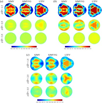
Phase-averaged axial velocity fields are reported in figure 5 at different cross-sections ( $z/D=1.5$,
 $z/D=2.5$,
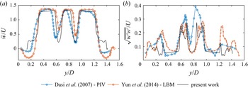
 $z/D=3.5$) of successive cycle stages, as they provide meaningful insights about the different flow features of the three cases investigated. In the PF stage the typical triple jet pattern is found to dominate the mean flow field, in agreement with previous investigations on SJMVs, both with straight (Guivier-Curien, Deplano & Bertrand Reference Guivier-Curien, Deplano and Bertrand2009; Hatoum, Maureira & Dasi Reference Hatoum, Maureira and Dasi2020) and anatomic (Ha et al. Reference Ha, Kim, Kweon, Lee, Kim, Kim and Yang2016) aortic root configurations. The streamwise mean velocity profile at PF, over the valve symmetry plane, replicates the trend observed in Dasi et al. (Reference Dasi, Ge, Simon, Sotiropoulos and Yoganathan2007) by PIV measurements and in Yun et al. (Reference Yun, Dasi, Aidun and Yoganathan2014a) by means of a lattice-Boltzmann computational approach. Actually, the mean flow field issuing from our simulations matches the maximum flow velocity and the width of the shear layer, whereas the backflow part of the profile is not represented. This is due to the significant differences in the geometric modelling of the aortic sinuses and in the valve orientation: it is clearly evident from figure 5(a) that the
 $y$-slice (centred on the valve axis) does not include recirculation regions. Analogous considerations can be drawn for the velocity root-mean-square (RMS) profile, bearing also in mind that different peak Reynolds numbers are involved in the comparison.
Dimensionless axial component  $\bar {w}/U$ of the mean flow field at subsequent cross-sections of the aortic root: (a) PF, (b) ED phase, (c) LD phase.

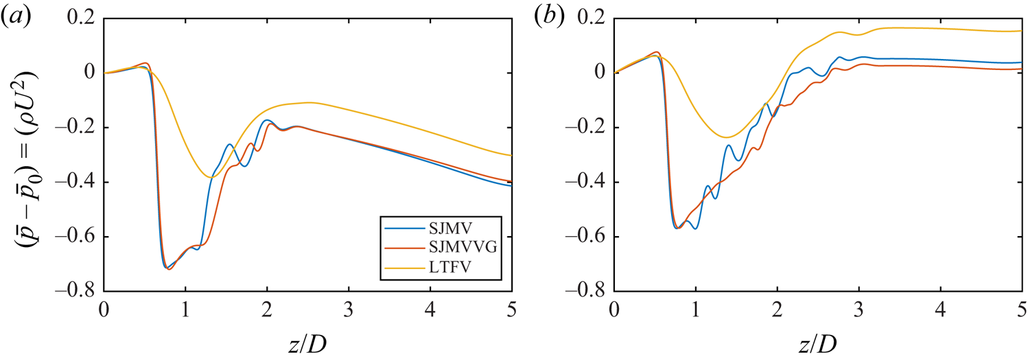
Streamwise distribution of phase-averaged pressure drop along the valve axis. (a) Peak flow rate. (b) Early deceleration.

The LTFV model instead provides four jets with a wider central jet. At this stage the recirculation regions reach the maximum intensity in all configurations, with axial velocity peaks of  $\bar {w}/U \approx -0.6$ in the SJMV and SJMVVG configurations, and
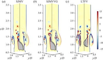
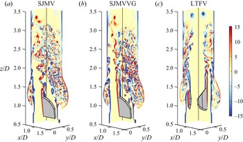
 $\bar {w}/U \approx -0.45$ in the LTFV. The reverse flow regions are observed to be localised in correspondence of the Valsalva sinuses in the bileaflet configurations, with the greatest intensity in the non-bisected sinus, in accordance with the prediction by Akutsu, Matsumoto & Takahashi (Reference Akutsu, Matsumoto and Takahashi2011). Conversely, the LTFV model provides a significantly lower amount of recirculation, being uniformly distributed in the near-wall regions of the aortic sinuses. Such a feature is a consequence of the installation of the LTFV leaflets within the housing (the reader should refer to figure 1), which puts the leaflets in a further forward position with respect to the aortic sinuses, when compared with the SJMV configuration. Thus, in the fully open position the LTFV leaflets shield the sinus cavity from the flow to create extended recirculation regions with large negative bulk flow velocity. This difference can be also perceived from the instantaneous vorticity fields over the valve longitudinal sections plotted in figures 7 and 8. At PF the LTFV jets propagate up to the streamwise position
 $z/D=2.2$ while holding their coherency. At ED the periodic vortex shedding triggered by the inflow rate reduction and by the development of the adverse pressure gradient in all models can be clearly identified in the instantaneous vorticity contours depicted in figure 8. In the ED stage the bileaflet valve jets extend up to the coordinate
 $z/D=3.5$ with reduced bulk velocity with respect to PF, while the characteristic triple jet pattern and the recirculation regions are maintained in space up to the coordinate
 $z/D=2.8$. In the bileaflet design the side jets impinge the aortic root generating a thin wall shear layer, whereas the trileaflet arrangement generates narrower lateral jets, symmetrically distributed in the azimuthal direction, which in turn provide a thicker wall shear layer. In section
 $z/D=2.5$ the central LTFV jet achieves a slightly larger bulk velocity (
 $\bar {w}/U \approx 0.90$) than the bileaflet lateral jets (
 $\bar {w}/U \approx 0.86$). It is worth pointing out that at ED the LTFV configuration shows significant changes in the topology of the mean flow between cross-sections
 $z/D=1.5$ and
 $z/D=2.5$. In the space of just one diameter the lateral jets disperse their momentum between the central jet and three circumferential jets generated from the interaction of the former with the structures shed from the housing. Again, a better understanding of the flow topology can be achieved comparing the mean flow (figure 5) with the instantaneous vorticity field (figure 8). In the LD phase the lateral jets of the SJMV model are still well separated in the aortic root, whereas the central jet starts to disintegrate due to the transition to turbulence. Instead, the circumferential jets observed at ED in the LTFV mix with the core jet to generate a three-lobed jet topology with
 $120^\circ$ symmetry. In section
 $z/D=2.5$ the bulk velocity of such a structure is almost unchanged from previous cycle instants, whereas the bulk velocity of bileaflet lateral jets has reduced to
 $\bar {w}/U \approx 0.79$. The same structure quickly breaks up as the jet advances downstream (
 $z/D=3.5$), introducing increased stochasticity in the flow behaviour. Immediately downstream of the leaflet both bileaflet cases produce strong reverse flow regions within the sinus cavity. On the contrary, the LTFV presents negative flow rate further downstream of the leaflets (
 $z/D=2.5$), which are not present in the other configurations.
Contours of instantaneous out-of-plane vorticity ( $\omega _x D/U$ and
 $\omega _y D/U$) over the longitudinal cross-sections of the aortic root in the PF stage.

Contours of instantaneous out-of-plane vorticity ( $\omega _x D/U$ and
 $\omega _y D/U$) over the longitudinal cross-sections of the aortic root in the ED stage.

The axial distribution of the mean pressure drop  $(\bar {p}-\overline {p_0})/(\rho U^2)$ along the valve axis is plotted in figure 6 at PF and ED, where
 $\overline {p_0}$ indicates the mean pressure at the inlet section. At PF, the transvalvular pressure drop (TPD) is assessed, corresponding to 0.629
 $\rho U^2$ (5.04 mmHg) for the SJMV model and 0.667
 $\rho U^2$ (5.35 mmHg) for the SJMVVG model. Conversely, the trileaflet valve provides a much smaller pressure drop, 0.390
 $\rho U^2$ (3.12 mmHg), owing to the presence of a wide central orifice. The TPD value found for the SJMV at PF matches the systolic gradient measured one year post-surgery, equal to 5.7 mmHg (St Jude Medical, Inc. 2010). No benchmark value for the TPD within a trileaflet valve is found. We found that LTFV is characterized by a smoother pressure recovery crossing the valve, while VGs bring a slight delay in the pressure recovery and negligible changes in the mean pressure drop. The minimal pressure increment with VGs is due to the further reduction of the orifice area.
It is worth noting that in our simulations we prescribe the same time-varying flow rate at the inflow boundary, and a radiative outflow condition at the outlet boundary for all valve models, whereas in the experimental set-up of Hatoum & Dasi (Reference Hatoum and Dasi2019), the flow rate emerges from the coupled problem, as a consequence of the pressure settling within the mock loop. Pressure recovery also depends critically on the root geometry that in our case includes the three sinuses of Valsalva, while in the experimental case it was straight (cylindrical). Although the VGs entail some differences in the mean flow field we emphasise that the cross-section contours in figure 5, as well as any other cuts of the mean flow field, do not provide a fully clear picture of the effect of the VGs on the flow field. Thus, we can speculate that they provide barely discernible differences on the phase-averaged mean flow, and we rely on instantaneous fields and second-order statistics to figure out the influence of these geometric appendices.
Ultimately, the observed mean flow fields contain some undamped vortical structures due to the relative brevity of the sampling time window, which is not wide enough to encompass the full characteristic period of the largest Kármán-like dipoles shed from the obstructions.
3.2. Fluctuating stress analysis
We illustrate stress distributions through the different valve configurations. Once acknowledged the ubiquitous nature of blood damaging mechanisms in turbulent flows (briefly mentioned in the introductory part of the manuscript), we limit our speculations to an Eulerian perspective of turbulent stresses. Reynolds stresses arise from the chaotic fluctuations primarily induced by the turbulent transition, and represent a fictitious stress contribution correlated with an enhanced blood damaging (Faghih & Sharp Reference Faghih and Sharp2019). A widely accepted conjecture postulates that abnormal flow conditions such as regurgitant jets and turbulent flows provide an instantaneous increase in viscous shear stress, exposure time and phase collision probability (Leverett et al. Reference Leverett, Hellums, Alfrey and Lynch1972; Antiga & Steinman Reference Antiga and Steinman2009; de Tullio et al. Reference de Tullio, Nam, Pascazio, Balaras and Verzicco2012). Hence, the evaluation of phase-averaged fluctuating stresses certainly provides a heuristic estimation of the stress levels experienced by blood elements, as well as the topology of the high-damaging regions. Although the fluctuating viscous stresses have been regarded as a far more appropriate metric than Reynolds stresses for quantifying blood damage (Ge et al. Reference Ge, Dasi, Sotiropoulos and Yoganathan2008), we argue that in a phase-averaging environment free from cycle-to-cycle variations, the latter provide a picture of the stochastic convective acceleration causing instantaneous enhancement in the viscous peak stresses and residence time experienced by blood constituents.
In the biomechanical literature the levels of both viscous and Reynolds stresses are often compared with haemolysis and platelet activation thresholds which have been obtained from a simple shear or extensional stress condition in laminar flows. The extension of these thresholds to turbulent stresses and complex stress states is fairly questionable, therefore, we interpret these thresholds as merely indicative.
A significant advantage of a numerical approach with respect to experimental investigations lies on the fact that three-dimensional evaluation of turbulent stress components can be performed without recurring to two-dimensional simplifying assumptions. In the experimental practice, the haemodynamic compliance of prosthetic heart valves is usually assessed from velocity information extracted over significant planes. However, the flow through a mechanical heart valve with realistic aortic root geometry was extensively proved to be fully three dimensional (Sotiropoulos & Borazjani Reference Sotiropoulos and Borazjani2009), as well as the turbulent stress distribution. Two-dimensional analysis has been proved to underestimate the normal and shear stresses, depending on the valve model and aortic root geometry (de Tullio et al. Reference de Tullio, Cristallo, Balaras and Verzicco2009). Since the peak Reynolds stress is not invariant under coordinate system rotation, a coordinate-independent metric is needed to quantify mechanical loads. Thus, we evaluate the full Reynolds stress tensor for every Eulerian node within the aortic root and compute the maximum turbulent shear stress (TSS) acting on a surface element (Malvern Reference Malvern1969) as the principal shear stress component
 \begin{equation} {\rm TSS}_{max}=\tfrac{1}{2} \left(\sigma_{max}-\sigma_{min} \right), \end{equation}
where  $\sigma _{max}$ and
 $\sigma _{min}$ represent the maximum and minimum principal normal stress components. It is recognised that flow through mechanical heart valves exhibits principal Reynolds normal stresses twice larger than the principal shear Reynolds stresses (Liu et al. Reference Liu, Lu and Chu2000; Nyboe et al. Reference Nyboe, Funder, Smerup, Nygaard and Hasenkam2006). However, the normal stresses are not regarded in this section since they are believed less harmful to RBC membrane (Faghih & Sharp Reference Faghih and Sharp2019). Here
 $\sigma _{max}$ and
 $\sigma _{min}$ can be obtained by solving the characteristic polynomial equation associated with the Reynolds stress tensor
 $\overline {u'_i u'_j}$,
 \begin{equation} \sigma^3-I_1 \sigma^2 + I_2 \sigma -I_3 =0, \end{equation}
being  $I_1$,
 $I_2$ and
 $I_3$ the second-order tensor invariants
 \begin{equation} \left.\begin{gathered} I_1 = \overline{u'_i u'_i}, \\ I_2 = \tfrac{1}{2} \left[\left(\overline{u'_i u'_i} \right)^2 - \overline{u'_i u'_i}^2 \right] , \\ I_3 = \tfrac{1}{6} \left(\overline{u'_i u'_i} \right)^3 - \tfrac{1}{2} \overline{u'_i u'_i}^2 \left(\overline{u'_j u'_j} \right)^2 +\tfrac{1}{3} \overline{u'_i u'_i}^3 . \end{gathered}\right\} \end{equation}
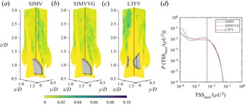
In order to provide a fair comparison among different valve models and different cycle instants we restrict the evaluation of the  $\textrm {TSS}_{max}$ to the interior node cloud from
 $z/D=0.8$ to
 $z/D=4.0$. Since the leaflet kinematics is prescribed, the velocity fluctuations at the solid–fluid interface are negligible. Before discussing the
 $\textrm {TSS}_{max}$ distributions, we highlight that the usefulness of the principal stress transformation to characterise fluid stresses for blood damage is uncertain and may depend on the local flow configuration, nevertheless, the complexity of the flow though prosthetic devices enables this descriptor as the most representative item for macro-scale evaluations.
The comparison carried out in figure 9 confirms that the level of accuracy achieved in our simulation guarantees a satisfactory agreement with experimental data both on first-order and second-order statistics. Figures 11–13 display two cutaway planes (corresponding to the spanwise planes  $XZ$ and
 $YZ$) of the three cases investigated with
 $\textrm {TSS}_{max}$ contours, along with probability density distributions of
 $\textrm {TSS}_{max}$, computed from three-dimensional fields. The interpretation of these figures can be facilitated by inspecting the streamwise distribution of turbulent kinetic energy (TKE), defined as
 $(\overline {u'_k u'_k})/U^2$, which is collected computing a RMS value at each cross-section (see figure 10). Previous experimental investigations on the SJMV model (Liu et al. Reference Liu, Lu and Chu2000; Hatoum et al. Reference Hatoum, Maureira and Dasi2020) found the peak systole to be characterised by the highest magnitude of
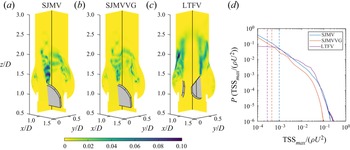
 $\textrm {TSS}_{max}$ within the cardiac cycle, whereas we identify a more complicated scenario. Certainly, the largest TKE RMS values are encountered at ED, whereas the phase location of the largest TSS
 $_{max}$ depends on the valve configuration. Such a discrepancy might be motivated by the difference in the boundary conditions governing the flow field, which in the experimental procedures consists of the pressure gradient applied by the hydrodynamic loop. At ED the TKE RMS peaks are found one diameter downstream of the leaflets for both SJMV and SJMVVG (see figure 10), whereas the LTFV provided similar peak values at PF and ED. In the PF SJMV configuration, the peak
 $\textrm {TSS}_{max}$ value, corresponding to a
 $10^{-5}$ probability density value, is found to be
 $(\textrm {TSS}_{max} /\rho U^2)_{P=1.0\times 10^{-5}}=0.142$, i.e. 151.4 Pa. The presence of VGs halves the same quantity to 0.0761 (81.15 Pa), whereas the LTFV generates similar values, namely 0.134 (142.9 Pa). Such values refer to a very limited event probability since they are confined to narrow spots in the flow field, located immediately downstream of the leaflets. A greater relevance in blood damage sourcing can be attributed to the volumetric median, whose values take 1.038, 0.479 and 0.294 Pa for the SJMV, SJMVVG and LTFV cases, respectively. This matches the experimental findings of Hatoum & Dasi (Reference Hatoum and Dasi2019) who correlated the reduction of the turbulent stress level in the co-rotating VGs arrangement with the reduction of vorticity intensity induced by the corruption of the most energetic coherent structures shed from the leaflet edges. This effect is captured in the
 $\textrm {TSS}_{max}$ contours in figure 12, where the VGs clearly mitigate the intensity of the stress spots connected to the large-scale vortex shedding, and it is reflected in a lower and spatially delayed TKE peak. In light of these findings, the additional instabilities brought by VGs seem to reduce the intensity of both normal and shear second-order fluctuations. The mechanism beyond such stress distribution and the spatial scales of the eddies that contribute to their production will be reinforced in the section concerning the spectral analysis. The LTFV configuration induces a similar peak value to SJMV, but a much lower median value, probably because the additional leaflet increases the probability of large stress levels. On the other hand, the limited mixing occurring in the LTFV entails narrower low-stress regions, mostly localised in the near-wall shear layer.
Profile of mean- and RMS value of the phase-averaged axial velocity component over the SJMV symmetry line at distance  $z/D=0.22$ from the leaflet tip, compared with data from literature, at PF.

Streamwise distribution of the cross-sectional RMS value of turbulent kinetic energy.

Contours of  $\textrm {TSS}_{max}$ over two spanwise cross-sections of the aortic root at the PF stage and probability density distribution computed from the corresponding three-dimensional field.

Contours of  $\textrm {TSS}_{max}$ over two spanwise cross-sections of the aortic root at the ED stage and probability density distribution computed from the corresponding three-dimensional field.

At ED, we find  $\textrm {TSS}_{max}$ peak values equal
 $0.131 \rho U^2$ (139.7 Pa) for the SJMV, and
 $0.119 \rho U^2$ (126.9 Pa) for the SJMVVG, mostly distributed in the leaflet wake and in the near-wall region at the sino-tubular junction. At this stage, where the vortex shedding from leaflet tips is fully developed, the stress level up to
 $z/D=1.5$ is much lower in the SJMVVG case than the SJMV case, due to the influence of VGs. Conversely, the LTFV provides a much lower peak stress level, with
 $(\textrm {TSS}_{max} / \rho U^2)_{P=1.0\times 10^{-5}}=0.0907$ (96.72 Pa), distributed on the edges of the core jet, which still preserve full coherency. This value is significantly larger than what was found by Hatoum et al. (Reference Hatoum, Maureira and Dasi2020), who denoted a
 $\textrm {TSS}_{max}$ peak of 72 Pa for the SJMV model, and approximately close to the values reported by Ge et al. (Reference Ge, Dasi, Sotiropoulos and Yoganathan2008) from three-dimensional numerical investigations. We stress that experimental evaluations based on two-dimensional velocity measurements provide systematically lower stress estimates. Differently, the computational investigation by Ge et al. (Reference Ge, Dasi, Sotiropoulos and Yoganathan2008) led to peak
 $\textrm {TSS}_{max}$ values close to 100 Pa. When comparing these values with the incipient haemolysis threshold brought to light from experimental correlations by Jhun et al. (Reference Jhun, Stauffer, Reibson, Yeager, Newswanger, Taylor, Manning, Weiss and Rosenberg2018), equal to 3000 Pa at
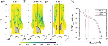
 $Re \ge 6 \times 10^4$, one might argue that the level of turbulent stress exerted on blood constituents across a BMAV are far below the critical value. However, they are recognised to be sufficient to induce significant sublethal damage to RBCs and platelet lysis for a given exposure time. In a representative study by Sutera (Reference Sutera1977), platelet clustering and lysis under shear load was found by simple shear tests for stress equal to 10 Pa. The transition to turbulence allows the bedding of the median stress level to 2.026 Pa for SJMV and SJMVVG, and to 0.906 Pa for the LTFV. The raise of the median values from PF to LD in all configurations bears witness to the transition to a distributed turbulent state across the computational domain. As the inflow rate decreases and a more uniform level of turbulent production occupies the downstream domain region, a larger probability of getting near-median stress values is observed, whereas the peak values are significantly reduced. At LD the peak and median stress values among the investigated cases conform to
 $0.0496 \rho U^2$ (52.89 Pa) and
 $0.00545 \rho U^2$ (5.81 Pa), respectively. It is worth noting that the LTFV provide a displaced TKE peak, at
 $z/D=2.7$, with respect to the other configurations (
 $z/D=1.9$), possibly caused by the fluctuations occurring in the formation of the tri-lobed jet observed in the mean flow at
 $z/D=2.5$ (the reader should refer to figure 5).
A statistical hypothesis testing is performed on the probability density distributions in figures 11–13, comparing SJMVVG and LTFV against the SJMV. The chi-square test provided  $p<0.001$, confirming that the null hypothesis is incorrect, therefore, the differences among the distributions can be considered statistically significant. The same outcome was obtained for all other distributions provided in the present work.
The picture of turbulence-induced flow environment experienced by RBCs can be completed by evaluating the fluctuating viscous stresses. These can be interpreted as the actual stress exerted on the volume element due to phase-averaged strain fluctuations. Following Jones (Reference Jones1995) the viscous stress distribution is evaluated by means of an equivalent scalar field  $\tau _{eq}$, named equivalent viscous stress (EVS) computed by double contraction of the fluctuating strain-rate tensor
 $s_{ij}$,
 \begin{equation} \tau_{eq}= \mu \sqrt{2 \overline{s_{ij} s_{ij}}}, \end{equation}
with  $s_{ij}=1/2 (\partial u'_i/\partial x_j + \partial u'_j/\partial x_i)$. Despite the fact that this information is deprived of the directionality of the stress, we rely on it because it comprises all the strain components, and because the majority of the stress-based models for haemolysis are built out of a scalar measure (Faghih & Sharp Reference Faghih and Sharp2019). Stress-based models are acknowledged to overestimate the damaging level, thus providing conservative estimates. Furthermore, the damaging level of blood constituents in high shear flows is affected by their degree of alignment with the flow direction (Goldsmith, Marlow & MacIntosh Reference Goldsmith, Marlow and MacIntosh1972) rather than the direction of the stress principal axis. Thus, we consider
 $\tau _{eq}$ a relevant and sufficiently general descriptor. It is worth noting that the EVS corresponds to the TKE dissipation rate
 $\varepsilon =2 \nu \overline {s_{ij} s_{ij}}$, by means of the relation
 $\tau _{eq}=\rho \sqrt {\nu \varepsilon }$. Thus, the EVS also depicts the rate at which the turbulence energy is dissipated by viscous forces.
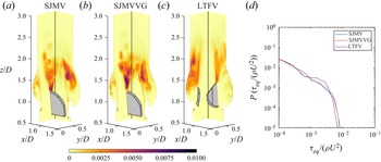
At PF fluctuating viscous stresses are localised in the near-leaflet wake, extending  $1.2D$ downstream of the trailing edge, as previously acknowledged by Yun et al. (Reference Yun, Dasi, Aidun and Yoganathan2014b) by inspecting the TKE dissipation rate contours. Likewise in simplified aortic root geometries (Ge et al. Reference Ge, Dasi, Sotiropoulos and Yoganathan2008; Yun et al. Reference Yun, Dasi, Aidun and Yoganathan2014b), a second viscous stress peak is found in correspondence of the housing edge, where the diffusion of the shear layer generates recirculation eddies constrained within the sinus cavity by the lateral jet. We denote from figure 14 the presence of these spots in all the configurations considered. Peak stress levels are identified with the same criteria used for
 $\textrm {TSS}_{max}$. However, we speculate that the intensity of the dissipation in the Valsalva sinuses strongly depends on the type of valve implantation. The LTFV presents the lowest EVS peak, corresponding to
 $0.00683 \rho U^2$ (7.28 Pa), whereas in the other configurations the EVS peak takes the approximate value
 $0.00797 \rho U^2$ (8.50 Pa). Since the EVS is negligible within most of the aortic root, the median values are lower than
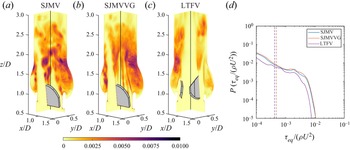
 $10^{-4} \rho U^2$ (0.107 Pa). The flow mechanisms characterising the ED make the peak stress value raise in all configurations, although larger increments are recorded for bileaflet cases. Specifically,
 $0.0106 \rho U^2$ (11.3 Pa),
 $0.0105 \rho U^2$ (11.19 Pa) and
 $0.00763 \rho U^2$ (8.13 Pa) for SJMV, SJMVVG and LTFV, respectively. In this phase the bileaflet models provide identical probability of the
 $\tau _{eq}$ event, although the spanwise contours in figure 15 show a larger shear stress in the early wake region in the SJMV. Once again this difference can be correlated with the reduced intensity of turbulent fluctuations brought by the VG arrays. The LTFV configuration generates definitively less viscous dissipation both in terms of peak and median value, mostly connected with the mixing of side jets and the core jet also noticed in the mean flow field (see figure 5).
Contours of  $\textrm {TSS}_{max}$ over two spanwise cross-sections of the aortic root at the LD stage and probability density distribution computed from the corresponding three-dimensional field.

Contours of  $\tau _{eq}$ over two spanwise cross-sections of the aortic root at the PF stage and probability density distribution computed from the corresponding three-dimensional field.

Contours of  $\tau _{eq}$ over two spanwise cross-sections of the aortic root at the ED stage and probability density distribution computed from the corresponding three-dimensional field.

Contours of  $\tau _{eq}$ over two spanwise cross-sections of the aortic root at the LD stage and probability density distribution computed from the corresponding three-dimensional field.

Throughout the cycle phases characterised by the largest TKE, in the leaflet wake, the maximum shear stress level falls well below the haemolysis threshold previously discussed in the turbulent shear stress assessment. On the other hand, the  $\tau _{eq}$ values recorded for the bileaflet cases are beyond the platelet activation threshold measured in Hung et al. (Reference Hung, Hochmuth, Joist and Sutera1976), corresponding to
 $10.0 \div 16.5$ Pa with an exposure time of 102 s, and in Ramstack, Zuckerman & Mockros (Reference Ramstack, Zuckerman and Mockros1979) corresponding to
 $30 \div 100$ Pa with an averaged residence time of 10 s. If relying on these thresholds, the LTFV can be regarded as less harmful for platelet activation. Eventually, the peak viscous stresses drop in the LD phase to the values 4.52 Pa for bileaflet cases and to 4.06 Pa for the LTFV (see figure 16).
An evaluation of the mean viscous shear stress could be useful to provide a broader picture of the flow stresses, and their correlation with the blood damage. However, these are not investigated since this study is mainly focused on the turbulence-induced stresses.
In view of the complex distribution of turbulent stresses, an integral interpretation would be impractical without considering more than one scalar quantity (Banerjee et al. Reference Banerjee, Krahl, Durst and Zenger2007), despite the fact they mostly act at a larger scale than the characteristic size of RBC (Antiga & Steinman Reference Antiga and Steinman2009). This is especially true in such a confined flow, at nearly transitional Reynolds number, where the uncertainty about the collocation of Reynolds stresses in the wavenumber space is much higher than simple isotropic homogeneous flows. To this extent, we quantify the level of anisotropy of turbulent stresses at ED and LD phases, where the transition to turbulence is definitely achieved.
The turbulent stress anisotropy is assessed by a colour mapping of the traceless anisotropy tensor  $B_{ij}$, defined by
 \begin{equation} B_{ij}=\frac{\overline{u'_i u'_j}}{\overline{u'_k u'_k}} - \frac{\delta_{ij}}{3}, \end{equation}
with  $\delta _{ij}$ being the Kroneker delta. The magnitude and orientation of turbulent fluctuations do conform, in a time-averaged sense, to specific states that can be characterised by a suitable mapping of the anisotropy tensor eigenvalues. Following Lumley & Newman (Reference Lumley and Newman1977), we explore the different turbulent states by building, at some relevant cross-sections, the anisotropy invariant map (AIM), whose coordinates are obtained as
 \begin{equation} C_{1C}=\lambda_1-\lambda_2, \quad C_{2C}= 2 \left( \lambda_2-\lambda_3 \right), \quad C_{3C}= 3 \lambda_3 + 1. \end{equation}
Here  $\lambda _i$ are the eigenvalues of
 $B_{ij}$, sorted in descending order, and
 $C_{iC} \ge 0$ are the eigenvalue-related weights of
 $B_{ij}$ in the appropriate tensor basis (Emory & Iaccarino Reference Emory and Iaccarino2014), making up the three turbulence corner states. To make broad-scale physical interpretations easier in our framework, we represent the AIM distribution at subsequent cross-sections of the aortic root by means of a contour representation whose scalar values are obtained assigning the RGB (Red-Green-Blue) colour triplet
 $[C_{1C},C_{2C},C_{3C}]$. This representation was proposed by Emory & Iaccarino (Reference Emory and Iaccarino2014), and named anisotropy componentality contours. Each component of the colour triplet represents the contribution to a AIM corner state (see figure 17), with corresponding stress shape: one-component turbulence (1C), two-component axisymmetric turbulence (2C) and isotropic turbulence (3C). The three borders joining the AIM corners provide intermediate limiting stages, described in figure 17. The global level of anisotropy of turbulent fluctuations at a certain cross-section is simply denoted by the anisotropy index, defined as
 \begin{equation} AI=\sqrt{\frac{1}{n} \sum_{i=1}^{n} (C_{1C}+C_{2C})_i^2} \end{equation}
over the  $n$ nodal locations within the observation domain.
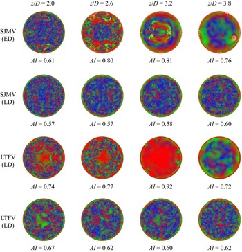
At ED the turbulent stresses show a high anisotropy level, with  $AI>0.75$ in section
 $z/D=2.6$, where the stresses mostly approach the one-component limit, both in the SJMV and LTFV configurations (see figure 18). At ED the cross-sections corresponding to
 $z/D=3.2$ and
 $z/D=3.8$ cannot be considered meaningful for this purpose because they do not lay in a region where significant turbulent fluctuations occur, so the related contours refer to the residual fluctuation being washed off the domain. In section
 $z/D=2.0$, which is pervaded by intense vorticity fluctuations at ED (see figure 8), the anisotropy level settles to
 $AI=0.61$ for SJMV and to
 $AI=0.74$ for LTFV. The former configuration presents a wide range of turbulent stress states uniformly distributed over the section, despite the presence of large shear layers in the mean flow field, depicted in figure 5. The latter instead provides a central region approaching the two-component limit, which makes the anisotropy index larger. At LD the anisotropy index is found to decrease and to become uniform across the domain to
 $AI \approx 0.6$ for both cases. In sections
 $z/D=2.6$ and
 $z/D=3.2$ the most elevated anisotropy occurred in correspondence of the shear layer surrounding the central jet, where the stress states are biased towards the one-component limit (1C), and the axisymmetric expansion bound. In the near-wall region, the stress states mostly approach the two-component limit, entailing a combination of red/green regions, as expected in the presence of a wall (Mansour, Kim & Moin Reference Mansour, Kim and Moin1988). The contours regarding the SJMVVG configuration are not reported here for the sake of brevity, since they provide a pattern very similar to that observed for the SJMV case. We speculate that despite the different vortex dynamics induced by the VGs, they do not affect the Reynolds stress directionality.
The considerations listed above on stress anisotropy provide a useful perspective for interpretation of spectral analyses, which are often carried out with the hypothesis of homogeneous isotropic flow.
3.3. Spectral analysis
In order to correlate the reduction in the turbulent stresses observed with the VGs to the large-scale vortex dynamics, we investigate the time spectra of instantaneous kinetic energy  $( u_i )^2/U^2$ at some points aligned with the SJMV leaflets in the fully open position. The LTFV configuration is excluded from this comparison. Figure 19 shows the time spectra of kinetic energy at the axial coordinates
 $z/D=1.5$ and
 $z/D=3.0$, averaged over the monitor lines 3, 5, 7, 9. Such spectra are computed from the velocity signal within a much larger cycle window than those considered for phase averaging in order to include the extended vortex shedding dynamics from PF
 $Q/Q_{max}=1.0$ to mid-deceleration
 $Q/Q_{max}=0.5$. In the leaflet shear layer the flow exhibits strong vortex shedding, with high energy content in the smaller temporal frequencies, whose dynamics is portrayed in figure 8 at ED. As the jets propagate further downstream, and the shear layers breaks up in favour of a mixing dynamics, the energy contained in the smaller frequency reduces by one order of magnitude. We emphasise that within the time window considered for signal sampling, the classical vortex shedding observed downstream of leaflets (Dasi et al. Reference Dasi, Ge, Simon, Sotiropoulos and Yoganathan2007) develops for both SJMV and SJMVG models, but the presence of the VGs leads to a lower energy content at all time scales, confirming that the associated co-rotating vortices locally disrupt the vortex rings periodically shed from the leaflet trailing edge in the high flow rate stage of the systole. Although this observation is provided from local evidences, we postulate that a similar pattern is consistently replicated in the leaflet tangent direction, explaining the significant reduction in the probability of large
 $\textrm {TSS}_{max}$ events at PF (see figure 11). This trend is reversed at the location
 $z/D=3.0$, where the SJMVVG provides larger kinetic energy, within a region were full transition occurred for both models. Further analysis on the energetic content of the purely fluctuating components are provided in the following by means of spatial spectra. One of the major motivations of this analysis is to correlate the turbulent stresses at different phases of the cardiac cycle with the geometry of the mechanical prostheses. Once the anisotropy pattern and the dissipative features occurring in the different configurations have been observed, the aforementioned correlations are sought by further investigating the spatial scales characterising the turbulent fluctuations in the frequency domain.
Barycentric colourmap of turbulent stress anisotropy.

Anisotropy componentality contours of the SJMV and LTFV configurations at the ED and LD stages, in subsequent aortic root cross-sections.

Time spectra of the kinetic energy at the axial coordinates (a)  $z/D=1.5$ and (b)
 $z/D=3.0$, averaged over the monitor lines 3, 5, 7 and 9.

Provided the strongly anisotropic nature of turbulent fluctuations we consider a local characterisation of the spatial fluctuations to be of greater impact in this application, therefore, power spectra are computed on the monitor lines (whose configuration is illustrated in figure 4), over segments starting downstream of the leaflets. A Hann window is applied to the velocity signals and the spatial average along the  $z$-direction is also subtracted. Line-averaged spectra are plotted for the streamwise TKE (figure 20), as well as for the anisotropic streamwise/leaflet-normal energy (figure 20) at three subsequent cycle instants. It can be immediately grasped that the energetic content of the turbulent fluctuations increases, especially at the largest spatial scales, as the inflow rate decelerates by the progressive shift of all curves towards higher energy levels. As the incoming flow rate decreases, the shear layers surrounding the core jet become more unstable due to the adverse pressure gradient, triggering a larger energy release towards smaller flow structures. None of the plotted spectra provide a clear classic scaling (Pope Reference Pope2001), despite the fact that a good fit with the inertial range scaling (
 $E_{ww}(k) \propto k^{-5/3}$) was identified already at the PF in previous studies (Yun et al. Reference Yun, Dasi, Aidun and Yoganathan2014b). In the present study the spatial spectral analysis is performed on localised lines within an anisotropic flow, which are not necessarily located where turbulence develops first or it is the strongest. Furthermore, one should bear in mind that at the PF instant most of the aortic root is crossed by residual low-energy structures that are immediately washed out in the acceleration phase. The recent experimental and numerical investigations by Cerbus et al. (Reference Cerbus, Liu, Gioia and Chakraborty2020), providing insights on local energy spectra for transitional pipe flow, reported that the power spectra (on-centreline and off-centreline) conforms to
 $-5/3$ scaling only for
 $Re \geq 80\,000$. Since the leaflets introduce a stronger degree of anisotropy in the flow than the simple free pipe, and the Reynolds number conforms to the transitional pipe regime, there is no reason to expect the Kolmogorov universal scaling laws.
Streamwise isotropic energy spectra at different cycle instants. Solid and dashed lines correspond to spectral values averaged over the inner and outer monitor lines annuli.

When considering the LTFV configuration, the inner line annulus fall within the central jet, which holds spatial coherency longer than the central jet ejected from the SJMV/SJMVVG models. As a matter of fact, the  $E_{ww}(k)$ spectrum mediated over the inner annulus has significantly lower energy content at the PF with respect to the outer annulus of the same model (see figure 20). At the ED/LD instants the energy distribution appears to be more uniform among the different configurations due to the enhanced mixing occurring in the deceleration phase. We emphasise that the intrinsic fluctuation associated with the energy-containing scales, corresponding to the largest wavenumber, at the ED/LD instants provides larger energy injection in the LTFV case, for both the inner and outer line annulus, owing to a more intense breakdown of the leaflet shear layer. These considerations apply both to the isotropic spectra and the shear spectra plotted in figure 21. We highlight that, differently from the isotropic spectra, the shear spectra, provide, especially in the LD phase, a better matching with the Lumley's scaling law, by which the small level of anisotropy in the inertial subrange can be assumed to be a small perturbation of the background isotropic state (Pope Reference Pope2001). This confirms that the strongly anisotropic nature of the fluctuations is lost in the central wavenumber range at LD, whereas a significant level of anisotropy characterises the intermediate length scales, and not only the energy-containing motion, at the PF and ED stages. It is worth pointing out the absence of energy pileup at high wavenumbers in any spectral representation, and the smoothness of the energy cascade which covers approximately nine orders of magnitude, meaning that most of the smallest flow scales are well represented without energy accumulation.
Anisotropic energy spectra at different cycle instants. Solid and dashed lines correspond to spectral values averaged over the inner and outer monitor lines annuli.

Our interpretation of the local energy spectra does not contradict the computational findings of Yun et al. (Reference Yun, Dasi, Aidun and Yoganathan2014b) and Becsek, Pietrasanta & Obrist (Reference Becsek, Pietrasanta and Obrist2020), that identified a clear inertial range from volume-averaged spectra collected over a wider flow rate interval. Since no clear indications on the fundamental micro-scales can be inferred from the energy spectra, we further inspect the nature of the fundamental scales involved in the flow field by computing the longitudinal Taylor micro-scale (LTMS) over the monitor lines. The Taylor micro-scale, denoted by  $\lambda$, represents the characteristic length of the largest eddies which are responsible for the dissipation of energy (Pope Reference Pope2001). Since the RBC membrane strain, which is a precursor to membrane failure, has a logical connection to surrounding fluid strain, the estimation of
 $\lambda$ might be relevant to haemolysis beyond any specific haemolysis mechanism (Faghih & Sharp Reference Faghih and Sharp2019). Longitudinal Taylor micro-scale is associated to the curvature of the velocity autocorrelation function. Thus, the longitudinal two-point correlation is computed for each line, at the generic streamwise location
 $z_0$ as
 \begin{equation} R_{ww}(z_0,\Delta z)= \overline{w'\left(z_0-\Delta z/2\right)w' \left(z_0+\Delta z/2\right)}. \end{equation}
This relation, once rescaled with respect to the velocity variance, provides the longitudinal autocorrelation function  $f_a(z_0,\Delta z)$. Then, for small separation
 $\Delta z$, the LTMS scale
 $\lambda (z_0)$ can be approximated by the roots of the osculating parabola of the autocorrelation function (Pope Reference Pope2001),
 \begin{equation} \lambda(z_0)=[-\tfrac{1}{2} f_a''(z_0,0)]^{-({1}/{2})}.\end{equation}
The second derivative in (3.9) is computed using a sixth-order accurate centred finite-difference scheme, using a seven-point stencil. This construction is carried out exploiting the symmetric correlation functions at different spots in between the streamwise coordinates  $z/D=2.0$ and
 $z/D=4.0$. Such a construction provides physically meaningful results for small values of
 $\lambda /\varLambda$ in homogeneous flows, with
 $\varLambda$ being the integral length scale (Belmabrouk & Michard Reference Belmabrouk and Michard1998). The influence of the additional terms appearing in higher-order expansions for non-homogeneous turbulence can be neglected for small
 $\Delta z$, namely, for a small deviation of the autocorrelation function from the osculating parabola (Belmabrouk & Michard Reference Belmabrouk and Michard1998).
In the present framework the evaluation of the LTMS does provide a cross-check on the dimension of the largest dissipative length scale with respect to energy spectra. Furthermore, we consider the LTMS to accomplish a more reliable estimation on fundamental scales than the Kolmogorov length scale, since the size of the smallest eddies might be affected by the local grid resolution. In contrast, the smallest LTMS observed, corresponding to  $\lambda /D=0.03$, can be overlaid onto approximately nine grid points, meaning that the corresponding eddy can be fully resolved with a second-order scheme. The axial coordinates
 $z_0$ from which the correlation functions are computed are chosen so that the zero-correlation condition is reached in a region of high vorticity. A polar map of the LTMS is reported in figure 22 for the three valve models analysed at the ED stage. In the SJMV and SJMVVG cases we identified a mean LTMS scale value of
 $\lambda /D=0.045$, corresponding to 1.0 mm. This value is approximately close to the length scale found by Yun et al. (Reference Yun, Dasi, Aidun and Yoganathan2014b), who identified the start of the energy decay at
 $l=3$ mm, from visual inspection of the energy spectra. Liu et al. (Reference Liu, Lu and Chu2000) obtained an experimental estimation of the LTMS, falling into the interval
 $\lambda =0.1\text{--} 0.6$ mm, computed by means of the velocity–time autocorrelation function, which was integrated from laser-Doppler anemometer measurements. They extracted the spatial LTMS approximating the spatial correlations by temporal correlations in view of the frozen field approximation (Taylor Reference Taylor1938). However, in pulsatile flows with a high degree of anisotropy this approximation is generally considered inaccurate (Pope Reference Pope2001). The LTFV configuration presented a larger LTMS, with a mean value of
 $\lambda /D=0.075$ at LD (see figure 23), corresponding to 1.73 mm. A larger LTMS value reflects the lower TKE RMS profile in figure 10, confirming that the trileaflet model produces a less energetic turbulence decay, with a larger dissipative structure, which can be thought to be less harmful to RBCs.
Polar map of the LTMS  $\lambda /D$ in the ED phase, at two different coordinates.

The mean LTMS value found from our analysis corresponds to the non-dimensional wavelength  $k/D \approx 130$, corresponding to a full energy decay region. No clear differences are generated by VGs, meaning that the different mixing mechanism at the energy-containing scales does not affect the dissipation in the smaller flow structures. The LTFV configuration provides highly non-homogeneous values, probably because the breaking of the shear layer carrying the jets mixing takes place further downstream with different energy content.
3.4. Outlooks and clinical implications
The present study can be further enhanced by including geometric features of a realistic aortic root reproducing the characteristic curvature of the ascending aorta. The non-planar shape of the root axis could introduce additional complexity to the flow field, as the swirl illustrated by Morbiducci et al. (Reference Morbiducci, Ponzini, Rizzo, Cadioli, Esposito, Montevecchi and Redaelli2011). The aortic arch can also generate secondary vortical regions which can potentially affect both mean flow field and fluctuations (Zhu, Seo & Mittal Reference Zhu, Seo and Mittal2018). Secondly, the adoption of pressure boundary conditions at the cross-flow domain edges certainly provides a more physiological flow evolution, especially if coupled with a lumped circulation model (Lee et al. Reference Lee, Rygg, Kolahdouz, Rossi, Retta, Duraiswamy, Scotten, Craven and Griffith2020), and consequently, a more realistic prediction of the flow features during valve closing (Dasi et al. Reference Dasi, Ge, Simon, Sotiropoulos and Yoganathan2007).
The FSI dynamics of a realistic valve model should include also the arterial wall elastic effects. A computational investigation by Hsu et al. (Reference Hsu, Kamensky, Bazilevs, Sacks and Hughes2014) proved that the flexibility of the aortic root damps out the fluctuations in the flow rate and attenuates leaflet oscillations in biologic valves. By mitigating these further sources of unsteadiness, we speculate that weaker turbulent fluctuations can be observed. Flamini, DeAnda & Griffith (Reference Flamini, DeAnda and Griffith2016) found that a compliant aortic wall substantially generates smaller peak pressure at systole and lower retrograde flow in the diastolic stage than those attained by rigid models. In the case of a mechanical prosthetic model with prescribed flow rate, limited differences in second-order statistics are expected.
The LTFV and SJMVVG models showed reduced turbulent stress levels if compared with the SJMV model, therefore, they can potentially replace it. However, this trend must be confirmed by clinical experimentation, which will involve further practical issues to account for. Concerning the VGs, their presence might induce a local accumulation of pannus and other fibrovascular tissues (Kim et al. Reference Kim, Choi, Kweon, Yang and Kim2020), which in turn can disrupt the associated haemodynamics. For this reason, the design of VGs must be limited to the simplest geometric elements. One possible investigation would require the application of a proper orthogonal decomposition method (De Cillis et al. Reference De Cillis, Cherubini, Semeraro, Leonardi and De Palma2021) to understand the topology of the modes responsible for the stress reduction and optimise the VGs collocation on the leaflets. We argue that in our study the VGs lay close to the leaflet leading edge, thus, they are subjected to the largest flow velocity. In this configuration the flow might wash the VGs surface and prevent the formation of biologic deposits, but this can be confirmed only by in-vivo experimentation. The VGs can guarantee improved haemodynamics without loosing decades of clinical experience with the SJMV model, since no large-scale design modifications are needed on the valve components. On the other hand, the LTFV certainly provides haemodynamic features closer to those of the natural valve, along with a noiseless closure. Older versions of a trileaflet valve were affected by the risk of leaflet sticking (Ghista Reference Ghista1976) which heavily influenced their development. However, the LTFV configuration is declared to guarantee an unimpeded leaflet opening (Novostia 2019).
Further analyses should address whether the beneficial haemodynamic effects of the VGs and LTFV hold for an intra-annular implantation. The reduced effective orifice area is expected to affect the TPD, the vorticity dynamics downstream of the leaflets as well as the recirculation within the Valvaslva sinuses. However, these arguments remain controversial (Kim et al. Reference Kim, Kim, Kim, Jung, Choo, Chung and Lee2019), and the related speculations should be confirmed by further analyses, especially in the presence of VGs.
4. Summary
The replacement of the aortic valve by a mechanical prosthesis still represents an issue of worldwide interest, since it involves a large portion of the 300 000 replacement procedures performed each year (Li Reference Li2019). Thus, the need for the improvement of the haemodynamics of mechanical valves raises from routine clinical practice. Direct numerical simulations of a pulsatile blood flow through three different MAV models have been conducted. Among them one configuration with VGs was investigated. The present numerical study proved that the influence of VGs and similar devices on the aortic root haemodynamics can be assessed with reasonable resolution and computational expense prescribing the leafled kinematics obtained from FSI computations.
The phase-averaged flow analysis revealed fundamental differences in the axial velocity field between bileaflet and trileaflet configurations, whereas no clear distinction is detected in the presence of VGs. Conversely, the mean pressure distribution pointed out a remarkable reduction in the pressure drop for the LTFV case, and a minimal pressure drop penalty with VGs.
Compared with previous experimental (Murphy et al. Reference Murphy, Dasi, Vukasinovic, Glezer and Yoganathan2010; Haya & Tavoularis Reference Haya and Tavoularis2016; Hatoum et al. Reference Hatoum, Maureira and Dasi2020) and computational (Ge et al. Reference Ge, Dasi, Sotiropoulos and Yoganathan2008; Yun et al. Reference Yun, Dasi, Aidun and Yoganathan2014b) studies, the major novelties lie in the detailed three-dimensional estimation of turbulent shear stresses and fluctuating viscous stresses. Arguments on the turbulent stress nature are supported by the characterisation of their directionality and by local spectral analyses. Since the main issue concerning BMAVs is the propensity to haemolysis and platelet activation, these have been compared with widely accepted thresholds (Faghih & Sharp Reference Faghih and Sharp2019), finding that the maximum turbulent shear stress value  $\textrm {TSS}_{max}$ falls below the threshold (
 $\ge$3000 Pa) highlighted in the most recent experimental campaign (Jhun et al. Reference Jhun, Stauffer, Reibson, Yeager, Newswanger, Taylor, Manning, Weiss and Rosenberg2018), by more than one order of magnitude. Our estimates are however consistent with those from other numerical investigations (Ge et al. Reference Ge, Dasi, Sotiropoulos and Yoganathan2008). The TSS
 $_{max}$ reach its peak value at PF in SJMV and LTFV models, whereas in the SJMVVG configuration the peak is achieved at ED, due to the vortex disruption brought by VGs. Despite this trend, both SJMV and SJMVVG models present the largest TKE RMS at the ED stage, where the transition to turbulence is definitely achieved. The largest EVS value is consistently reached in the ED phase in all configurations, when the largest dissipation is expected. Visual inspection of cross-section contours revealed that the presence of VGs increases the EVS at PF and decreases magnitude in the ED stage. The LTFV is the only model providing EVS below the platelet activation threshold (
 $\tau \leq 10$ Pa, following Sutera Reference Sutera1977), although the other configurations showed moderately exceeding values. Inspection of the Reynolds stress anisotropy revealed a significant level of anisotropy in the decelerating phase, with
 $AI > 0.60$, providing a landmark for the interpretation of energy spectra. The LTFV presented a slightly larger anisotropy index at all cross-sections. The local evaluation of TKE spectra did not match the classic Kolmogorov scaling laws, but illustrated an increase in the energy content per wavenumber with the advancement of inflow deceleration. The scale analysis was carried out by computing locally the LTMS, which showed a mean value equal to 1 mm for bileaflet configuration and 1.7 mm for the LTFV. This confirms the tendency of the trileaflet design to generate larger dissipative structures, with consequently lower risk of RBC membrane damaging.
Polar map of the LTMS  $\lambda /D$ in the LD phase, at two different coordinates.

Acknowledgements
The simulations were carried out on the high performance computing infrastructure of the Department of Mechanics Mathematics and Management, Polytechnic University of Bari (Italy). The authors would also like to thank Dr D. Passiatore and Dr S. De Carolis for their useful comments in the development of this work.
Funding
This work has been partially supported by Italian Ministry of University and Scientific Research (MIUR) via PRIN2017 XFAST-SIMS grant no. 20173C478N.
Declaration of Interests
The authors report no conflict of interest.
Appendix A. FSI computations
The present investigation has been carried out relying on a prescribed inflow rate and leaflet kinematics, in order to reduce the computational expense. The magnitude of the numerical endeavour was guaranteed by the necessity of achieving a sufficient grid resolution to resolve the smallest turbulent structures, as well as by the requirement to simulate enough cardiac cycles to collect statistically converged data. In this connection, one preliminary FSI simulation has been run for each valve configuration with a two-way coupling setting. Only three cardiac cycles have been run, and the leaflet motion in the third cycle has been used to extract the kinematic laws to enforce in one-way coupled simulations. One-way coupled simulations allowed us to reduce the computational expense related to the integration of loads over the leaflet surface, along with the computation of the MLS transfer functions at runtime. Our preliminary simulations guarantee that instantaneous inflow rate and leaflet's instantaneous angle of attack are fully consistent, provided that negligible cycle-to-cycle variations are observed in the leaflet kinematics. This was widely verified when constraining the inflow rate.
Equations of rigid body motion are integrated by an explicit Adams–Bashforth scheme with variable time step size. The leaflet volume moment of inertia  $J_0/D^5$ about the rotation axis is equal to
 $4.444 \times 10^{-4}$ for the SJMV,
 $4.454 \times 10^{-4}$ for the SJMVVG, and
 $2.154 \times 10^{-4}$ for the LTFV. Leaflets are assumed to be made of pyrolytic carbon (St. Jude Medical, Inc. 2010), therefore, the density ratio
 $\rho _s/\rho =1.887$ is assigned. Figure 24 shows that the presence of VGs does not bring significant differences in the leaflets kinematics. Such a small difference is motivated by the fact that the leaflet opening follows an impulsive dynamics, being almost insensitive to small variations in the moment of inertia. Furthermore, VGs bring a 0.2 % change in the volume moment of inertia, being collocated in correspondence of the rotation axis. Our computations confirmed the earlier closing of the trileaflet configuration, experimentally observed by Vennemann et al. (Reference Vennemann, Rösgen, Heinisch and Obrist2018). Variations induced by the VGs are slightly magnified when considering the torque exerted on the single leaflet (see figure 25).
Net rotation angle on a single leaflet resulting from FSI computations.

Comparison of non-dimensional torque  $T/(\rho U^2 D^3)$, superposed with the non-dimensional angular velocity
 $\dot {\theta } D/U$, on a single leaflet for the opening (a) and closing phase (b). Axes scales are magnified to highlight the differences among curves.

Appendix B. Grid convergence study
The flow in this study is resolved by a DNS approach, therefore, it is fundamental to establish whether the mesh employed is able to capture all of the relevant flow structures. In this connection, a grid convergence study is conducted on the SJMV model with the VGs, since it is expected to generate smaller dissipative scales with respect to the trileaflet valve, and it provides smaller geometric features (the VGs themselves) than the standard SJMV model. Three different meshes with uniform spatial resolution equal to  $301 \times 309 \times 961$ (coarse),
 $421 \times 439 \times 1401$ (baseline) and
 $519 \times 533 \times 1731$ (fine) are employed to solve the same problem. The ratios of computational cell volume between different grids are
 $V_{{coarse}}/V_{{baseline}}=1.4$ and
 $V_{{baseline}}/V_{{fine}}=1.24$. It is worth noting that the baseline grid provides 278 nodes overlapping the tissue annulus diameter (which represents the characteristic geometric scale of the problem) and 12 nodes overlapping the leaflet thickness. As already mentioned in § 2.2, a similar resolution is employed in Yun et al. (Reference Yun, Dasi, Aidun and Yoganathan2014b) on the same problem with a different numerical approach but similar spatio-temporal accuracy of the numerical scheme. In the baseline grid the VGs are overlapped by 34 grid points in the length direction and nine in the height and thickness. Data are collected after four cardiac cycles to deal with the cost of more refined computations. As shown in figure 26, the streamwise component of the mean flow at the PF stage provides significant similarities in the two most refined cases. The baseline grid is able to reproduce the core jet velocity as well as the width of the shear layer of the fine grid. The level of accuracy of the predictions obtained at affordable cost with the baseline grid has been demonstrated in the comparison of this profile with experimental data (see figure 9), although the amount of cycles is not sufficient to precisely compute second-order statistics. Furthermore, the choice of a CFL-controlled time-stepping strategy makes the number of samples collected within each stage window remarkably different for different grids (the reader should refer to the discussion in § 2.3). This significantly affects the comparison among the considered meshes.
Mean streamwise velocity profiles at the section  $z/D=1.5$ in the PF stage. Results are shown for the (a) YZ plane; (b) XZ plane.

Appendix C. Convergence of ensemble statistics
The statistical samples are collected in correspondence of three different cycle instants by means of the ensemble averaging described in § 2.2. The amplitude of the time interval centred in each cycle instant of interest is selected a priori from the inflow rate curve by identifying the time slot corresponding to a  $\pm$1.0 % flow rate variation. In this connection, the amplitude of each time slot, thus the amount of frames collected, depends on the slope of the inflow rate curve. Hence, a different number of snapshots are collected for different cycle instants, leading to a potential non-uniform reliability of statistical measurements. Specifically, at the PF, where the largest time sampling window occurs with
 $T_{{PF}}=0.47 U/D$, we collected approximately
 $1180$ time samples per cycle, whereas at the ED, where
 $T_{{ED}}=0.13 U/D$, we collected approximately
 $440$ samples per cycle. To overcome this issue, we run the simulations for enough cardiac cycles to obtain a statistical convergence through all cycle instants with respect to a predefined threshold. A similar sampling strategy was employed by Yun et al. (Reference Yun, Dasi, Aidun and Yoganathan2014a), collecting data over a single cardiac cycle, within a time window defined by the integral time scale, computed by means of the Kolmogorov estimate
 $\tau _i=\tau _{\eta } \sqrt {{Re}}$ (Pope Reference Pope2001). It is worth noting that such an estimate provides at the PF the value
 $\tau _i=58.7$ ms, based on
 $Re=5780$, which is larger than our dimensional time range
 $T_{PF}=10.8$ ms.
The convergence of the first-order and second-order statistics is locally inspected over the monitor lines schematically depicted in figure 4, by measuring their cycle-to-cycle variation. Figure 27 displays the root mean square error (RMSE) of the change in the streamwise mean flow velocity from cycle  $N-1$ to cycle
 $N$, where the RMSE operator is applied twice, over all cells crossed by a monitor line, and over all monitor lines, to get a non-local convergence indicator. Such a parameter shows a clear convergence trend in the streamwise mean flow, since it can be considered within an asymptotic region at the 18th cycle at the three successive cycle phases under examination. Thus, local cycle-to-cycle variations of
 $\bar {w}$ are several orders of magnitude lower than the estimated mean value. Furthermore, the streamwise distribution of relative monitor line-averaged variation from the 17th to the 18th cycle is provided for the SJMVVG and LTFV models in figure 28. Such a distribution provides a mean variation equal to
 $0.2\,\%$ with peaks of
 $0.7\,\%$ for all models. This determines a good agreement with the experimental practice described in Ha et al. (Reference Ha, Kim, Kweon, Lee, Kim, Kim and Yang2016), which declared uncertainties due to incomplete convergence around
 $0.1\,\%$ for the streamwise velocity, although their phase-averaged refers to a time window comprising a much larger portion of the systolic phase. Both graphs suggest that the LD cycle instant provides the largest statistical uncertainty, owing to the largest streamwise velocity fluctuations. This is because at PF and ED instants the flow field is essentially laminar in the rear part of the domain, where the residual vortical structures have been rapidly washed out of the domain, as depicted in figure 5, thus leading to a more rapid convergence. Similar observations are provided with respect to second-order statistics, and specifically to the Reynolds stress tensor component
 $\overline {w'w'}$ (see figures 29 and 30). The same statistical descriptor used for the mean flow shows that the asymptotic range is achieved by the 18th cycle, where a corresponding mean uncertainty equal to
 $3\,\%$ is accepted. This is consistent with the uncertainty found by Ha et al. (Reference Ha, Kim, Kweon, Lee, Kim, Kim and Yang2016) on second-order statistics too.
Cycle-to-cycle evolution of the RMSE of the change in the streamwise mean flow velocity.

Streamwise distribution of relative monitor line-averaged variation in the streamwise velocity component from the 17th to the 18th cycle.

Cycle-to-cycle evolution of the RMSE of the change in the isotropic streamwise Reynolds stress component.

Streamwise distribution of relative monitor line-averaged variation in the isotropic streamwise Reynolds stress component from the 17th to the 18th cycle.

It is worth highlighting that the first cycle is excluded from the phase-averaging process since the flow field is initialised with uniform velocity.