1. Introduction
During vertical launching, as shown in figure 1, an underwater vehicle progresses through three distinct phases: the launching stage, underwater navigation and water-exit, ultimately completing the entire trajectory (Zhang et al. Reference Zhang, Li and Jin2005; Zhang, Yao & Zhang Reference Zhang, Yao and Zhang2013; Wang & Huang Reference Wang and Huang2018; Shi et al. Reference Shi, Ren, Gao and Pan2022b ). During the launching stage, the underwater vehicle is propelled by high-pressure gas towards the free surface, and finally exits the launcher tube. Subsequently, an air mass forms that bridges the vehicle’s bottom wall and launcher tube exit. This air mass then ruptures, forming (i) a mobile tail cavity that adheres to the vehicle, and (ii) a remaining air mass that is stationary near the launcher tube exit (Zhou & Yu Reference Zhou and Yu2017; Cheng et al. Reference Cheng, Quan, Zhang, Zhang and Li2022b ; Yao et al. Reference Yao, Qu, Ma, Yang, Quan and Cheng2023). In addition, to maintain orientation stability, artificial ventilation is applied to generate ventilated shoulder cavities to fully envelop the underwater vehicle (Nguyen et al. Reference Nguyen, Phan, Duy and Park2022; Zhang, Lyu & Fan Reference Zhang, Lyu and Fan2022). As a result, both tail and ventilated cavities simultaneously attach to the vehicle and interact dynamically, leading to cavity shedding, tail cavity rupture, and other unsteady effects that complicate the launching process (Chen et al. Reference Chen, Shi, Pan and Shan2021a ). Therefore, a thorough understanding of the coupled evolution of ventilated shoulder and tail cavities is essential for optimising the design of vertically moving underwater vehicles.
The process of underwater launching.

Initially, artificial ventilation was widely applied for horizontally moving vehicles. By blowing non-condensable gas into the low-pressure region at the shoulder, ventilated cavities can considerably reduce skin friction drag on underwater vehicles. When these cavities grow large enough to envelop most of the vehicle body, they enable high-speed movement (Epshtein Reference Epshtein1973; Logvinovich Reference Logvinovich1973; Zhao et al. Reference Zhao, Wang, Wei and Zhang2015; Sun et al. Reference Sun, Zhang, Zhang, Jiang and Zong2019). To date, water tunnels have served as an effective experimental platform for investigating ventilated cavitation. The platform enables systematic variation of flow conditions across a broad range of key parameters, including cavity pressure (
 $P_C$
), ambient pressure (
 $P_{atm}$
), incoming velocity (
 $U$
), and ventilation flow rate (
 $Q$
). These parameters commonly correspond to the following dimensionless groups: cavitation number
 ${\sigma _c} = ( {P_{atm} - {P_C}} )/ ( {0.5\rho {U^2}} )$
, air entrainment coefficient
 ${C_Q} = Q/U{D^2}$
, Froude number
 $\textit{Fr} = U/\sqrt {g{D^2}}$
, where
 $D$
,
 $g$
and
 $\rho$
denote feature size, gravitational acceleration and water density, respectively. In studies of ventilated cavities, gas leakage is an important phenomenon. Non-condensable gas escapes from the rear sealing region during the evolution of the ventilated cavity, resulting in multiple closure modes, such as re-entrant jet (Semenenko Reference Semenenko2001; Kshatriya, Patwardhan & Eaglesham Reference Kshatriya, Patwardhan and Eaglesham2007), twin vortex (Spurk Reference Spurk2002), pulsating cavity (Skidmor Reference Skidmor2013) and quad vortex (Kapankin & Gusev Reference Kapankin and Gusev1984; Kawakami & Arndt Reference Kawakami and Arndt2011). Subsequent researches have extensively investigated the underlying fluid mechanisms governing these closure modes. For example, Karn, Arndt & Hong (Reference Karn, Arndt and Hong2016) confirmed that gravity served as a main factor in the generation of the twin vortices, resulting in vortex stretching and tilting processes. This caused the cavity to lift in the streamwise direction, creating a velocity difference between the upper and lower cavity surfaces, which led to subsequent flow separation. Moreover, through further experiments in a recirculating cavitation water tunnel at Saint Anthony Falls Laboratory, Karn et al. (Reference Karn, Arndt and Hong2016), Shao et al. (Reference Shao, Wu, Haynes, Arndt and Hong2018) and Jiang, Shao & Hong (Reference Jiang, Shao and Hong2018) have established connections among the dimensionless parameters governing the above-mentioned closure modes. To obtain detailed flow field characteristics, Wang et al. (Reference Wang, Huang, Zhang, Wang and Zhao2018) and Barbaca et al. (Reference Barbaca, Pearce, Ganesh, Ceccio and Brandner2019) utilised proper orthogonal decomposition methods to analyse coherent flow structures, including shear layers induced by Kelvin–Helmholtz instability. In addition, numerical studies, such as direct numerical simulations (Liu, Xiao & Shen Reference Liu, Xiao and Shen2023) and large-eddy simulations (LES) (Xiong et al. Reference Xiong, Wang, Dong, Wang and Zhang2024), were also conducted to comprehend the flow mechanism of ventilated cavities.
Different from horizontally moving underwater vehicles, cavity evolution around a vertically moving underwater vehicle remains in a transient state with limited travel distance; the direction of gravity acts parallel to the vehicle’s axial direction rather than radially. Without flow control, a natural cavity will adhere to the surface of the vehicle. During water-exit , the collapse of the natural cavity induces significant structural loading on the vehicle body, consequently compromising trajectory stability (Zhao et al. Reference Zhao, Sun, Zhang and Yao2014; Wang et al. Reference Wang, Huang, Fang, Wu and Du2016; Fu et al. Reference Fu, Zhao, Sun and Lu2018; Gao et al. Reference Gao, Shi, Pan and Quan2022b
). Therefore, artificial ventilation is required to mitigate these adverse effects, enabling successful water-exit for underwater vehicles (Wang & Huang Reference Wang and Huang2018). To generate ventilated cavities from the shoulder region to cover the vehicle surface, Zhang (Reference Zhang2018), Hu (Reference Hu2018) and Gong (Reference Gong2018) jointly designed a ventilation system. Using this system, Chen et al. (Reference Chen, Xiao, Gong, Yao and Hu2022) observed various closure modes for the ventilation cavities, including foamy cavity re-entrant jet twin vortex closure. However, the ventilated cavities obtained in their study, which featured large radial dimensions, were significantly affected by boundary conditions, resulting in extremely asymmetric cavity shape. To address this limitation, Qu et al. (Reference Qu, Yang, Ma, Yao and Chen2022) and Gan et al. (Reference Gan, Liu, Yao, Chen, Ma and Cui2022a
,
Reference Gan, Yao, Cheng, Chen and Mab
) optimised both the experimental set-up and the underwater vehicle shape, investigating the effects of key parameters (e.g.
 $\textit{Fr}$
,
 $C_Q$
and
 $\sigma _c$
) on ventilated cavity evolution. They demonstrated that during water-exit, the non-condensable gas in ventilated cavities modified collapse behaviour and significantly reduced impact pressure compared to natural cavities. Considering the limited information obtained from experiments, Ma et al. (Reference Ma, Chen, Yu and Liu2018, Reference Ma, Chen, Yu, Wang and Jiang2019) and Gan et al. (Reference Gan, Yao, Su and Cui2022c
) employed the finite volume method to examine internal flow field structures within ventilated cavities. These investigations revealed various vortex structures, including shear-layer vortices and horseshoe vortices, which were found to significantly influence gas–liquid interface instability and subsequent flow pattern. Based on the potential flow theory, Li et al. (Reference Li, Sun, Xiao and Yao2019a
,
Reference Li, Sun, Yao and Piaob
, Reference Li, Sun, Yao and Wu2020) adopted the boundary element method to investigate three-dimensional ventilated cavity evolution under vertically incoming flow. Their results demonstrated that reduced surface tension significantly exacerbates cavity deformation. Ren et al. (Reference Ren, Wang, Quan and Cheng2023) explored the impact of head shape on ventilated cloudy cavities, demonstrating that abrupt curvature variations in the head region attenuate inertial effects, thereby promoting the generation and detachment of cloudy ventilated cavities.
As initially discussed, the vertical launching process is a complex procedure involving the coupling of ventilated and tail cavities. Early works for tail cavities were conducted by Zhang et al. (Reference Zhang, Xu, Wang, Lu and Zhao2017) and Xu et al. (Reference Xu, Wang, Lu and Huang2018) in the Harbin Institute of Technology HT01 Ventilation Cavity Water Tunnel. Similar works were later carried out by Cheng et al. (Reference Cheng, Quan, Sha, Yang, Wang and Xu2022a), Yang et al. (Reference Yang, Wang, Wei, Wang, Zhang and Hu2022a,b, 2023) and Quan & Cheng (Reference Quan and Cheng2023). They installed a nozzle at the bottom of an underwater vehicle to eject supersonic or subsonic gas jets to generate ventilated tail cavities, and identified multiple types of cavities, including intact, foam, pulsating foam and broken cavities. To establish correlations among the dimensionless parameters governing the aforementioned tail cavity shapes, Xu et al. (Reference Xu, Wang, Lu and Huang2018) and Zhao et al. (Reference Zhao, Xiang, Zhang, Liu and Li2021) modified the traditional jet–cavity coupling model originally introduced by Paryshev (Reference Paryshev2006) and Kirschner et al. (Reference Kirschner, Moeny, Krane and Kinzel2015). Their analysis revealed that the relative position between closure point of ventilated tail cavities and the iso-line of
 $P_{0}=P_{0f}$
dominated tail cavity shapes, where
 $P_{0}$
and
 $P_{0f}$
denoted the stagnation pressure and total incoming pressure, respectively. Considering vertically incoming flow, Qu et al. (Reference Qu, Yang, Ma, Yao, Zhang, Zhang, Cheng and Quan2023) demonstrated the influence of surface tension coefficient
 $S$
(expressed through the Weber number
 $We = \rho {U^2}D/S$
) on ventilated tail cavity morphology. Their results showed that a decrease in
 $We$
intensified gas–liquid mixing at the cavity rear, and diminished air mass entrainment capacity, ultimately triggering foam cavity shedding. Extending this work, Yao et al. (Reference Yao, Wang, Ma, Zhang, Chen, Qu, Zhang, Lu and Zhang2024) installed tail wings onto underwater vehicles to stabilise ventilated tail cavities, providing insights for deeper-water launch applications.
In vertical launching scenarios, a tail cavity forms as the vehicle leaves the air-filled launcher tube. The gas inside the tube, driven by inertia, follows the vehicle’s upward motion and adheres to its bottom wall, thereby forming a tail cavity (see figure 1). Different from ventilated tail cavities, this type of cavity lacks a continuous gas supply after initial formation. Thus its morphology becomes difficult to maintain during subsequent transient evolution, leading to gas–liquid interface instability (Gao et al. Reference Gao, Shi, Pan and Quan2022c
,
Reference Gao, Shi, Pan, Quan and Lud
). To investigate the hydrodynamic characteristics of tail cavities, Yao et al. (Reference Yao, Qu, Ma, Yang, Quan and Cheng2023) designed a vertical launching experimental set-up featuring scaled model testing. Compared with the open water tank designed by Wang et al. (Reference Wang, Huang, Du, Fang and Liang2012) and Sun, Sun & Zhao (Reference Sun, Sun and Zhao2014), this set-up employed an air compressor to control ambient pressure
 $P_{atm}$
, significantly mitigating scale effects. Experimental observations revealed distinct pulsation modes of the tail cavity during vertical launching: expansion, over-expansion, contraction and over-contraction. With an increase in cavity pulsation cycles, the cavity’s gas entrainment capacity decreased progressively, leading to cavity shedding. Subsequently, a cooperative group of Yao et al. (Reference Yao, Qu, Ma, Yang, Quan and Cheng2023) conducted a systematic investigation into the underlying fluid mechanisms governing these observed phenomena. Zhao et al. (Reference Zhao, Yao, Zhao, Ma, Fang, Zhang, Shi and Ji2024) found that the cavitation number
 $\sigma _c$
and tail cavity pulsation shared similar frequencies, only lagging by one phase. This also indicated that the pressure gradient across the cavity interface served as the primary driver of cavity pulsation. Ren et al. (Reference Ren, Wang, Cheng, Quan and Yu2024) investigated the fluid mechanism governing cavity shedding, establishing a direct correlation between cavity shedding and vortex shedding. Their results demonstrated that U-shaped vortex and vortex ring shedding triggered foamy cavity shedding, whereas hairpin vortex shedding induced vortex tube shedding. It should be noted that these studies were limited to single launching, while practical engineering applications typically employ continuous launching to maximise operational efficiency. Lu et al. (Reference Lu, Bi, Wang, Wei, Wang and Zhang2022a
,
Reference Lu, Wang, Song, Wei, Yu and Lib
) experimentally investigated the impact of launch time interval on continuous launching. Their results demonstrated that an extended time interval significantly reduced the interference with the attitude of subsequently launched vehicles. However, constrained by experimental limitations, Lu et al. (Reference Lu, Bi, Wang, Wei, Wang and Zhang2022a
,
Reference Lu, Wang, Song, Wei, Yu and Lib
) were unable to explain the underlying fluid mechanisms. Numerical simulations performed by Gao et al. (Reference Gao, Shi, Pan and Quan2022a
) and Shi et al. (Reference Shi, Gao, Pan and Quan2022a
,
Reference Shi, Ren, Gao, Pan and Quanc
) revealed that hairpin vortices generated in the vehicle’s wake region created a low-speed streak zone, leading to a reduction in both hydrodynamic force and pressure coefficients on subsequently launched vehicles. An increase in launch time interval significantly decreased the influence of the low-speed streak region, stabilising the attitude of subsequent vehicles.
Previous research primarily focused on tail cavities and ventilated cavities as separate phenomena (Gui et al. Reference Gui, Chuang, Wei, Sun and Yang2021; Sun et al. Reference Sun, Zhang, Wei, Zhang and Zhang2022). However, underwater vertical launching is a complex process coupling these two types of cavities. Thus based on our prior works (Ren et al. Reference Ren, Wang, Quan and Cheng2023, Reference Ren, Wang, Cheng, Quan and Yu2024, Reference Ren, Wang, Quan, Cheng, Cheng and Cheng2025), the current work presents detached-eddy simulations (DES) to investigate the cavity flow under vertical launching conditions, focusing on the interaction between the ventilated shoulder and tail cavities. This work is new and challenging. We aim to explore the underlying mechanisms of the interaction between the shoulder and tail cavities.
The remainder of this paper is organised as follows. Section 2 presents the numerical methods and parameter configurations employed in this study. Section 3 discusses the pulsation process of the tail cavity without considering the shoulder cavity. Section 4 subsequently investigates interactions between the tail and shoulder cavities, while § 5 examines how shoulder ventilation rates influence these interactions.
2. Methodology
This section presents the simulation set-up process. First, we introduce the division of the computational domain, followed by the grid generation strategy and the applied grid techniques. We conclude with the governing equations for numerical simulation.
2.1. Computational domain
To investigate the interaction between the shoulder and tail cavities, we employ a geometrically scaled underwater vehicle model (
 $1:40$
) rather than a full-scale prototype. This ensures sufficient grid resolution for cavity simulation within feasible computational resources. As shown in figure 2(a), a complete three-dimensional computational domain is established. The computational domain for the underwater navigation phase is rectangular, with a reference frame established at the centre of the launcher tube exit. The computational domain spans
 $2L$
in the horizontal directions (
 $x$
and
 $y$
), and extends
 $5L$
in the vertical direction (
 $z$
). The upper and outer boundaries are set as the pressure outlet conditions, and the bottom boundary is set as a wall condition. The computational domain of the launcher tube is shown in figure 2(b). The underwater vehicle, with a cylindrical geometric shape and an elliptical nose, is assumed to move at a constant speed opposite to the gravity direction. The vehicle’s slenderness ratio is 6 : 1 (length
 $L=330\,\rm mm$
, diameter
 $D=55\,\rm mm$
). The air seam, serving as a mass flow inlet for non-condensable gas discharge to generate a ventilated shoulder cavity, is installed at the vehicle’s shoulder zone. The launcher tube is cylindrical, with diameter
 $D$
and length
 $1.5L$
. The tube’s lateral wall is set as a wall boundary condition. As the vehicle passes through the launcher tube, constant internal pressure is maintained via a pressure outlet condition at the tube bottom. Upon exiting the tube, the boundary condition transitions to a wall condition, terminating gas supply.
Division of computational domains. (a) Rectangular computational domain, where
 $L$
and
 $D$
represent the length and width of the vehicle, respectively,
 $u_v$
is the velocity of the vehicle, and
 $Q$
is the ventilation rate. (b) Computational domain of the launcher tube.

In the current work, several dimensionless parameters are defined to determine the initial conditions and for subsequent data analysis.
The Froude number
 $\textit{Fr}$
is
 \begin{equation} \textit{Fr} = \frac {u_v}{{\sqrt {gL} }}, \end{equation}
where
 $\textit{Fr}$
is employed to determine the velocity of the vehicle
 $u_v$
.
The cavitation number
 $\sigma$
is
 \begin{equation} {\sigma } = \frac {{{P_{atm}} - {P_v}}}{{0.5{\rho _w}{U^2}}}, \end{equation}
where
 $P_v$
is the saturated vapour pressure of water. Here,
 $\sigma$
is used to determine the atmospheric pressure
 $P_{atm}$
.
The dimensionless launching pressure
 $P_r$
is
 \begin{equation} {P_r} = \frac {{{P_{in}}}}{{{P_{atm}} + \rho g{H_0}}}, \end{equation}
where
 $P_r$
is used to determine the initial pressure of the launcher (
 $P_{in}$
) during the launching stage.
The dimensionless ventilation flow rate
 $\bar Q$
is
 \begin{equation} \bar Q = \frac {Q}{{{u_v}{L^2}}}, \end{equation}
where
 $Q$
is the ventilation flow rate on the air seam.
The dimensionless displacement of vehicle movement
 $\bar H$
is
 \begin{equation} \bar H = \frac {{H}}{L}, \end{equation}
where
 $H$
is the vertical location of the vehicle’s bottom wall.
The dimensionless pressure
 $\bar P$
is
 \begin{equation} {\bar P} = \frac {{P - [{P_{atm}} + \rho g({H_0} - H)]}}{{{P_{atm}} + \rho g{H_0}}}, \end{equation}
where
 $P$
is the pressure of the fluid field.
The average dimensionless pressure at the bottom wall of the vehicle
 $\bar P_B$
is
 \begin{equation} {\bar P_B} = \frac {{{P_B} - [{P_{atm}} + \rho g({H_0} - H_B)]}}{{{P_{atm}} + \rho g{h_0}}}, \end{equation}
where
 $H_B$
is the vertical location of the vehicle’s bottom wall.
Based on geometric scaling,
 $\textit{Fr}$
is the primary dynamic similarity law, which results in a velocity scaling relationship
 $u_{vm}=\sqrt {\lambda }\, u_{vp}$
, where
 $\lambda$
is the scale ratio
 $1/40$
, and
 $u_{vm}$
and
 $u_{vp}$
denote the velocities of the model and prototype vehicles, respectively. The similarity of
 $\sigma$
yields a pressure scaling
 $P_{atmm}-P_{v}=\lambda (P_{atmp}-P_{v})$
, where
 $P_{atmm}$
and
 $P_{atmp}$
are atmospheric pressures of the model and prototype vehicles, respectively. The dynamic similarity laws are developed based on works of Chen et al. (2021b) and Ma et al. (Reference Ma, Zhang, Sun, Shi, Yao, Yang and Qu2023), and are aconsistent with our previous studies (Ren et al. Reference Ren, Wang, Quan and Cheng2023, Reference Ren, Wang, Cheng, Quan and Yu2024). In fact, scaled-down simulation is also adopted as a practical approach to obtain more detailed flow field information under the constraints of limited computational resources. Moreover,
 $P_r$
is used to characterise the initial pressure inside the launcher tube during the launching stage. Here,
 $\bar H$
,
 $\bar P$
and
 $\bar P_{B}$
are employed for quantitative analysis. Table 1 summarises the initial conditions of numerical cases presented in this paper.
Initial conditions of each case in the present numerical simulations.

2.2. Grid division and technique
To prevent gas leakage during the launching stage, which can affect the evolution of cavities, the diameter of the launcher tube is set equal to that of the underwater vehicle in this simulation. Therefore, a zero-gap overlapping grid technique (Shi et al. Reference Shi, Gao, Pan and Quan2022a
) is applied to address the treatment of overlapping wall boundary conditions. The technique deactivates the wall boundary grid and establishes a temporary interface between the corresponding regions, thereby ensuring the stability of the numerical simulation during the launching stage. Figure 3 illustrates the grid division strategy. The mesh height for the first layer is
 $5.0 \times {10^{-7}}\rm m$
at the vehicle boundary, and
 $5.0 \times {10^{-6}} \rm m$
at the launcher tube boundary, with corresponding growth rates 1.1 and 1.2. The average grid size
 $\varDelta _{\textit{avg}}$
in the vehicle’s movement region is 1.5 mm, and the time step is set as
 ${\varDelta _{\textit{avg}}}/ ( {10U} )$
. Grid independence verification and mesh details are provided in Appendix A.
To provide sufficient resolution of the gas–liquid interface and accurately capture the unsteady evolution of cavities, adaptive mesh refinement (AMR) technology is employed. As shown in figure 4, the grid is refined by two levels in regions where the volume fraction of water
 $\alpha$
ranges between 0.2 and 0.8, and the vertical position
 $z$
is between
 $0L$
and
 $2.5L$
. In addition, the octree method is adopted for grid refinement, and data interpolation is performed for data transfer between the coarse and fine grids.
Grid division. The grids in the background and overlapping regions are represented in black and red, respectively. The geometric model is shown in blue.

Strategy of AMR. The simulation result is obtained from case 1 at
 $\bar H=0.20$
, where
 $\bar H$
is the dimensionless vertical position of the vehicle’s bottom wall. The iso-line of 90 % water volume fraction is used to illustrate the tail cavity shape.

2.3. Numerical methods
Based on the finite volume method, the interaction between shoulder and tail cavities is simulated using the commercial computational fluid dynamics software STAR-CCM+. The fluid field is modelled as a two-phase flow (water and gas), with natural cavitation effects neglected. Air is modelled as a compressible ideal gas, while water is treated as an incompressible fluid. The air phase follows the ideal gas law
 $P={\rho }RT$
, where
 $P$
is the pressure,
 $\rho$
is the air density,
 $R$
is the gas constant with value
 $287\ \rm J\ kg^{-1}\ K^{-1}$
, and
 $T$
is the absolute temperature. The specific heat ratio is defined as
 $\gamma = {C_P}/{C_v}$
, where
 $C_P$
is the specific heat at constant pressure with value
 $1005\ \rm J\ kg^{-1}\ K^{-1}$
, and
 $C_v$
is the specific heat at constant volume. The volume of fluid method (Hirt & Nichols Reference Hirt and Nichols1981) is employed for the multiphase flow calculation, with a high-resolution interface capture scheme for discretising the convective flux in the volume of fluid transport equation (Gao et al. Reference Gao, Shi, Pan and Quan2022c
). The DES method (Spalart et al. Reference Spalart, Deck, Shur, Squires, Strelets and Travin2006) is used for the turbulence calculation. Using DES is a hybrid turbulence modelling approach that combines Reynolds-averaged Navier–Stokes (RANS) simulations and LES. The governing equations are introduced below.
The volume fraction equation is
 \begin{equation} \frac {{\partial {\alpha _k}}}{{\partial t}} + \boldsymbol{\nabla} \boldsymbol{\cdot} ({\alpha _k}\boldsymbol {u}) = 0. \end{equation}
The continuity equation is
 \begin{equation} \frac {{\partial {\rho _m}}}{{\partial t}} + \boldsymbol{\nabla} \boldsymbol{\cdot} ({\rho _m}\boldsymbol {u}) = 0. \end{equation}
The momentum equation of RANS simulations is
 \begin{equation} \frac {{\partial {\rho _m}{\boldsymbol {u}}}}{{\partial t}} + \boldsymbol{\nabla} \boldsymbol{\cdot} \left ( {{\rho _m}\boldsymbol {u} \otimes \boldsymbol {u}} \right ) = - \boldsymbol{\nabla} \boldsymbol{\cdot} {p}\boldsymbol {I} + \boldsymbol{\nabla} \boldsymbol{\cdot} \left ( {\bar {\boldsymbol {T}} + {{\boldsymbol {T}}_{\textit{RANS}}}} \right ) + \boldsymbol {F}. \end{equation}
The momentum equation of LES is
 \begin{equation} \frac {{\partial {\rho _m}\tilde {\boldsymbol {u}}}}{{\partial t}} + \boldsymbol{\nabla} \boldsymbol{\cdot} \left ( {{\rho _m}\tilde {\boldsymbol {u}} \otimes \tilde {\boldsymbol {u}}} \right ) = - \boldsymbol{\nabla} \boldsymbol{\cdot} {\tilde p}\boldsymbol {I} + \boldsymbol{\nabla} \boldsymbol{\cdot} \big( {\tilde {\boldsymbol {T}} + {{\boldsymbol {T}}_{\textit{SGS}}}} \big ) + \boldsymbol {F}, \end{equation}
where
 ${\alpha _k}$
denotes the volume fraction of each phase,
 $\rho _m$
is the mixture density of fluid,
 $\boldsymbol {u}$
is the RANS velocity,
 $\tilde {\boldsymbol {u}}$
is the LES filtered velocity,
 $\tilde p$
is the filtered pressure,
 $\boldsymbol {T}$
is the mean viscous stress tensor,
 $\tilde {\boldsymbol {T}}$
is the filtered stress tensor,
 ${\boldsymbol {T}}_{\textit{RANS}}$
is the Reynolds-stress tensor,
 ${\boldsymbol {T}}_{\textit{SGS}}$
is subgrid-scale stress tensor, and
 $\boldsymbol {F}$
is the body force term.
The present simulation employs the shear stress transport (SST)
 $k\text{-}\omega$
model (Menter Reference Menter1994) for RANS simulations, which is a two-equation model that considers the transport of turbulence shear stress and introduces the blending function. The governing equations of the SST
 $k\text{-}\omega$
model are
 \begin{align}& \frac {{\partial {\rho _m}k}}{{\partial t}} + \boldsymbol{\nabla} \boldsymbol{\cdot} \left ( {{\rho _m}k\boldsymbol {u}} \right ) = \boldsymbol{\nabla} \boldsymbol{\cdot} \left [ {\left ( {{\mu _m} + {\sigma _k}{\mu _t}} \right )\boldsymbol{\nabla} k} \right ] - {f_{{\beta ^*}}}{\beta ^*}{\rho _m} \tilde \omega k + {P_k}, \end{align}
 \begin{align}& \frac {{\partial {\rho _m}\omega }}{{\partial t}} + \boldsymbol{\nabla} \boldsymbol{\cdot} \left ( {{\rho _m}\omega \boldsymbol {u}} \right ) = \boldsymbol{\nabla} \boldsymbol{\cdot} \left [ {\left ( {{\mu _m} + {\sigma _\omega }{\mu _t}} \right )\boldsymbol{\nabla} \omega } \right ] - {f_\beta }\beta {\rho _m}{\omega ^2} + {P_\omega }, \end{align}
where
 $k$
is the turbulent kinetic energy,
 $\mu _m$
is the dynamic viscosity of the mixture,
 $\mu _t$
is the turbulent viscosity,
 $\omega$
is the turbulent frequency,
 $\sigma _k$
and
 $\sigma _\Omega$
denote the turbulent model constants,
 $f_\beta$
is the vortex-stretching modification factor,
 $f_{{\beta ^*}}$
is the shear modification factor,
 $\beta$
and
 $\beta ^*$
are model coefficients, and
 $P_k$
and
 $P_\omega$
are production terms. Notably,
 $\omega$
is modified to address the problem of modelled stress depletion (Spalart et al. Reference Spalart, Deck, Shur, Squires, Strelets and Travin2006; Shur et al. Reference Shur, Spalart, Strelets and Travin2008), which can occur when the separation region is narrow or the boundary layer is thick. In the current simulation, the semi-implicit method for pressure-linked equations (SIMPLE) is used to solve the pressure–velocity coupling in the flow field. Both time and spatial terms are discretised using a second-order upwind scheme. In addition, the surface tension model is employed (Xiong et al. Reference Xiong, Wang, Dong, Wang and Zhang2024), and the surface tension coefficient is taken as
 $0.072\rm \,N\,m^{-1}$
.
The evolution process of tail cavities without shoulder cavities attached. (a) The flow patterns of tail cavities. The iso-surface of 90 % water volume fraction is used to illustrate the tail cavity shape. (b) The variation of cavity volume and
 $\bar P_{B}$
with
 $\bar H$
.

3. The evolution of tail cavities without shoulder cavities attached
In this section, simulation results for case 1 are presented to investigate the flow characteristics of tail cavity pulsation in the absence of shoulder cavities. The flow patterns of tail cavities are shown in figure 5(a). At
 $\bar H=0.23{-}0.71$
, the underwater vehicle initially leaves the launcher tube while remaining connected to it by an air mass. As the vehicle moves towards the free surface, the air mass undergoes necking and eventually ruptures, forming a tail cavity attached to the vehicle’s bottom wall. Subsequently, the tail cavity initiates its unsteady evolution process. Regarding flow patterns, the tail cavity undergoes periodic expansion and contraction. During transitional phases between pulsation cycles (specifically during contraction-to-expansion transitions), large-scale cavity shedding occurs at the tail cavity’s rear portion (as marked in figure 5
a). The variation of cavity volume and
 $\bar P_{B}$
with
 $\bar H$
is provide in figure 5(b). At
 $\bar H=0.00{-}0.74$
, the underwater vehicle remains connected to the launcher tube via an air mass. Initially, the air mass internal pressure significantly exceeds the ambient pressure, driving rapid cavity volume expansion. As internal pressure progressively decreases below ambient pressure, the cavity volume contracts, leading to the air mass rupture, evidenced by a distinct discontinuity in the cavity volume curve at
 $\bar H=0.74$
. Following this rupture, a tail cavity forms and attaches to the bottom wall of the vertically moving vehicle. Pressure differences between the interior and exterior of the tail cavity drive periodic cavity pulsations, characterised by continuous expansion–contraction cycles. In addition, throughout the entire underwater navigation process, the volume of the tail cavity continues to increase due to the ambient pressure reduction caused by vertical movement.
The expansion of the air mass at
 $\bar H=0.14$
. (a) The flow pattern of the air mass. (b) The contour of dimensionless pressure
 $\bar P$
. The iso-line of 90 % water volume fraction is used to illustrate the air mass shape. The velocity field is in reference to the underwater vehicle. (c) Scheme of fluid particle motion.

The contraction of the air mass at
 $\bar H=0.50$
. (a) The flow pattern of the air mass. (b) The contour of dimensionless pressure
 $\bar P$
. The iso-line of 90 % water volume fraction is used to illustrate the air mass shape. The velocity field is in reference to the underwater vehicle. (c) Scheme of fluid particle motion.

The pulsation process of the tail cavity, where
 $\boldsymbol{\nabla} \boldsymbol{\cdot} (\boldsymbol{V}{\rho _m})$
represents the mass flux. A positive value of
 $\boldsymbol{\nabla} \boldsymbol{\cdot} (\boldsymbol{V}{\rho _m})$
indicates expansion of the cavity shape, whereas a negative value indicates contraction. In addition, the iso-line of 90% water volume fraction is used to illustrate the tail cavity shape.

Figures 6 and 7 illustrate the detailed flow field during air mass necking, where a positive value of the dimensionless pressure
 $\bar P$
indicates that the internal air mass pressure exceeds the ambient pressure, whereas a negative value indicates the inverse relationship. In figure 6, the pressure inside the air mass substantially exceeds ambient pressure, resulting in an expansion trend of the air mass . At this position, the underwater vehicle leaves the launcher tube with a constant speed, and drives the internal gas to move along with it. However, constrained by the incoming flow with high kinetic energy, the flow direction deflects upon impinging on the vehicle’s bottom wall, and subsequently turns downstream. In comparison, the fluid near the tube exit imposes weaker constraints on the air mass, making it the primary region of expansion. Additionally, due to the abrupt change in curvature, a large-scale vortex forms at the tube exit. As the air mass continues to expand, its internal pressure gradually drops below the ambient pressure, thereby initiating the contraction process. As shown in figure 7, the moving vehicle is capable of carrying only a limited amount of trailing fluid. As the air mass begins to contract, the residual fluid within it, defined as the returning flow, starts to move downstream and re-enters the launcher tube. The most pronounced necking of the air mass during contraction occurs at the location where the flow direction changes, as this region offers the weakest resistance to contraction. As the necking progresses, the air mass eventually ruptures, leading to the formation of a tail cavity.
To investigate the pulsation mechanism of the tail cavity,
 $\boldsymbol{\nabla} \boldsymbol{\cdot} (\boldsymbol{u}{\rho _m})$
is applied to quantitatively characterise the expansion and contraction processes. A positive value of
 $\boldsymbol{\nabla} \boldsymbol{\cdot} (\boldsymbol{u}{\rho _m})$
indicates cavity expansion, whereas a negative value indicates contraction. As shown in figure 8, expansion and contraction coexist within the tail cavity. This is a distinct phenomenon, differing from the typical pulsation behaviour of bubbles in a free flow field (Zhang et al. Reference Zhang, Li, Cui, Li and Liu2023). On the one hand, under vertical launching conditions, the tail cavity exhibits a large size in the direction of gravity, resulting in significant variations in ambient pressure along its length. On the other hand, as displacement gradually increases, water pressure continuously decreases. These factors cause the transitions between cavity expansion and contraction to consistently occur in the upstream region of the tail cavity. Meanwhile, in the downstream region, the cavity remains in a state of contraction due to greater water depth. In figure 8, at
 $\bar H=0.95$
, the internal pressure of the upstream cavity exceeds the ambient pressure, causing expansion. At
 $\bar H=1.04$
, as the cavity volume increases, the internal pressure gradually drops below the ambient pressure. However, the marked cavity region in figure 8(b) continues to expand due to inertia effects, a phenomenon referred to as over-expansion. At
 $\bar H=1.13$
and
 $1.31$
, the tail cavity undergoes sequential contraction and over-contraction. This indicates that the change in cavity volume is a relative process. When the rate of expansion exceeds the contraction, the volume of the tail cavity increases; conversely, the cavity volume decreases. Based on the characteristics of volume variation, figures 8(a), 8(b), 8(c) and 8(d) are defined as expansion, over-expansion, contraction and over-contraction, respectively, which together constitute a complete pulsation cycle. In addition, due to over-expansion and over-contraction, the change of cavity volume usually lags behind the change of pressure. As the tail cavity pulsation repeats, cavity shedding occurs. As shown in figure 9, at
 $\bar H=1.73$
, the rear of the tail cavity undergoes continuous compression due to the combined effects of ambient pressure and stagnation high pressure. Ultimately, the tail cavity is cut off, leading to cavity shedding and the generation of significant shear stress, as marked in figure 9(b). In addition, a new stagnation high-pressure point forms at the location where cavity shedding occurs.
The process of cavity shedding. The iso-line of 90 % water volume fraction is used to illustrate the tail cavity shape.

Through the above mechanistic analysis, a more precise understanding of the tail cavity pulsation process is obtained. However, when considering the presence of the shoulder cavity, particularly when it extends to the region of the tail cavity, how do the two cavities interact? This issue is discussed in the next section of this study.
4. The analysis of the interaction between ventilated and tail cavities
In this section, case 2 is set as a typical working condition to analyse the interaction between shoulder and tail cavities. The cavity flow patterns during the underwater navigation stage are exhibited in figure 10. Before the underwater vehicle exits the launcher tube, non-condensable gas is expelled through the air seam to form the shoulder cavity. However, owing to the buoyancy effect and the high momentum of the non-condensable gas, the initial radial size of the shoulder cavity is relatively large at
 $\bar H=-0.46$
. Subsequently, flow separation at the end of the shoulder cavity causes this portion of the cavity to gradually contract and eventually shed at
 $\bar H=0.08$
. The detached cavity moves downstream and interacts with the air mass near the launcher tube exit, leading to earlier rupture and greater instability of the gas–liquid interface compared to conditions without shoulder cavity attachment (case 1). At
 $\bar H=0.62$
, the shoulder and tail cavities encounter the bottom wall of the underwater vehicle. Subsequently, the shoulder and tail cavities merge, forming a supercavity attached to the vehicle surface.
The cavity evolution in case 2. The iso-surface of 90 % water volume fraction is used to illustrate the tail cavity shape.

The variation of
 $\bar P_{B}$
with
 $\bar H$
under the comparison of cases 1 and 2. Case 1 takes into account the attachment of the shoulder cavity, whereas case 2 does not.

Additionally, the variation modes of pressure at the bottom wall are critical to the success of underwater launches, and represent one of the primary focuses of this study. Figure 11 shows the variation of
 $\bar P_{B}$
with
 $\bar H$
for cases 1 and 2. Before
 $\bar H=0.67$
, the variation modes of
 $\bar P_{B}$
in the two cases are similar. However, after this point, the variation modes of
 $\bar P_{B}$
diverge completely. As described in § 3, in case 1, the pressure pulsation is driven primarily by the contraction and expansion of the tail cavity, without the attachment of a shoulder cavity. When the shoulder cavity is taken into consideration (case 2), the frequency of pressure pulsation increases significantly. However, the underlying fluid mechanics of this phenomenon remain unclear.
In the following subsections, this interaction process is decomposed into various stages, with different analytical methods employed.
4.1. The fusion process of the shoulder and tail cavities
Figure 12 shows the details of the flow field at
 $\bar H=0.68$
in case 2. At this location, although the re-entrant jet at the end of the shoulder cavity causes fluid particles to move upstream, the distance between the shoulder and tail cavities is too large for the re-entrant jet to influence the flow pattern of the tail cavity. Consequently, the tail cavity remains unable to break through the confinement and expand towards the lateral wall. As the shoulder cavity continues to propagate, it approaches and interacts with the tail cavity. As shown in figure 13, the re-entrant jet from the shoulder cavity induces fluid particles near the tail cavity boundary to move towards the vehicle’s lateral wall, thereby initiating the fusion process between the shoulder and tail cavities.
Details of the flow field at
 $\bar H=0.56$
in case 2. (a) The flow pattern of the cavity. (b) The flow field of the marked region. The iso-line of 90 % water volume fraction is used to illustrate the cavity shape. (c) Scheme of fluid particle motion.

Details of the flow field at
 $\bar H=0.68$
in case 2. (a) The flow pattern of the cavity. (b) The flow field of the marked region. The iso-line of 90 % water volume fraction is used to illustrate the cavity shape. (c) Scheme of fluid particle motion.

Fusion process of the shoulder and tail cavities in case 2.

Subsequently, the tail cavity continues to develop upstream, while the shoulder cavity progresses downstream, ultimately leading to their encounter. However, as shown in figure 14, due to the influence of surface tension, the two cavity boundaries do not fully merge but instead form a boundary resembling a liquid film, referred to as the fusion line (FL). Affected by the FL, the upstream motion of the fluid particles is impeded, leading to the formation of a large-scale vortex in front of the FL (at
 $\bar H=0.7015$
). At the same time, the tail cavity drives the FL to continue moving upstream. During the process, part of the FL disappears, and the two regions gradually merge. Some fluid particles from the tail cavity converge into the vortex in front of the FL, while others continue to move upstream towards the shoulder cavity. Eventually, the two cavities completely merge, and the FL disappears.
The impact of the shedding cavity on the tail cavity evolution, where
 $\boldsymbol{\nabla} \boldsymbol{\cdot} (\boldsymbol{u}{\rho _m})$
represents the mass flux. A positive value of
 $\boldsymbol{\nabla} \boldsymbol{\cdot} (\boldsymbol{u}{\rho _m})$
indicates an expansion of the cavity shape, whereas a negative value indicates contraction. In addition, the iso-line of 90 % water volume fraction is used to illustrate the cavity shape.

The process of the tail cavity being cut off by the shoulder cavity in case 2. The left-hand side shows the contour of water phase. The right-hand side is a schematic illustration, with red and blue lines indicating the two directions of fluid particles motion within the tail cavity.

4.2. The impact of shoulder cavity on the flow pattern of the tail cavity
As previously exhibited in figure 10 (
 $\bar H=0.14{-}1.11$
), the influence of the shoulder cavity on the evolution of the tail cavity can be divided primarily into two stages: before and after the shoulder cavity extends to the location of the tail cavity.
Before this, under the combined effects of buoyancy and incoming flow, a small portion of the cavity detaches from the shoulder cavity and moves downstream along the vehicle (Ren et al. Reference Ren, Sun, Li and Wei2021). As this shedding cavity encounters the tail cavity, it intensifies the instability of the gas–liquid interface of the tail cavity (as shown in figure 15 b). By comparing figure 15(a), which represents the condition without the shoulder cavity attached (case 1), it is found that the shedding cavity accelerated the velocity of the surrounding fluid, thereby increasing the contraction rate of the downstream cavity. At the same time, the contraction rate of the upstream cavity significantly decreases. The significant difference in the contraction rates along the gas–liquid interface causes the instability on the interface.
After that, the tail cavity is gradually cut off by the shoulder cavity (as exhibited in figure 10 at
 $\bar H=0.80$
). Figure 16 presents the detailed process. At
 $\bar H=0.71$
, upon the encounter of the shoulder and tail cavities, the motion of fluid particles diverges into two directions: one portion flows upstream towards the shoulder cavity, while the other merges into the downstream region, forming a small-scale vortex and leading to a reduction in the radial dimension of the tail cavity. At
 $\bar H=0.74$
, as the cavity develops, the vortex size gradually increases, continuously compressing the radial dimension of the tail cavity, and ultimately leading to its rupture and the formation of the supercavity.
In order to quantitatively analyse the velocity field, the dimensionless relative velocity
 $\bar u_{\textit{ref}}$
and height
 $\bar H_{\textit{ref}}$
are defined as
 \begin{align}&\quad {\bar u_{\textit{ref}}} = \frac {{{u_{\textit{ref}}}}}{{\sqrt {gl} }}, \end{align}
 \begin{align}& {\bar H_{\textit{ref}}} = \frac {{{H_c} - H}}{L}, \end{align}
where
 $u_{\textit{ref}}$
is the velocity of the flow field relative to the vehicle, and
 $H_c$
is the vertical position of the origin (as marked on the right-hand side of figure 17
a). As shown in figures 17(a) and 17(b), after the fusion of the tail and shoulder cavities, the first rupture occurs following the tail cavity necking. At the rupture position, flow separation occurs. One part continues to move in the direction of the incoming flow, while the other part moves towards the vehicle’s bottom wall along the re-entrant flow, forming stagnation high-pressure point I. Eventually, the re-entrant flow impacts the vehicle’s bottom wall, forming stagnation high-pressure point III. In the subsequent cavity evolution, the tail cavity is completely cut off by the shoulder cavity, and the vehicle is enveloped by the supercavity at
 $\bar H=0.89$
. At the position of the second rupture, stagnation high-pressure point III forms. As shown in figures 17(a) and 17(c), on the one hand, point III drives the fluid to accelerate upstream; on the other hand, it decelerates the fluid driven by point I. As the vehicle continues to move, the influence of point I gradually decreases, and the re-entrant flow is driven primarily by point II.
(a) The variation of
 $\bar u_{\textit{ref}}$
with
 $\bar H_{\textit{ref}}$
in the vehicle’s wake region. The right-hand side shows the cavity shape at the corresponding position, with the range of
 $\bar u_{\textit{ref}}$
. (b) The contour of
 $\bar u_{\textit{ref}}$
, with diagram at
 $H=0.83$
. (c) The contour of
 $\bar u_{\textit{ref}}$
, with diagram at
 $H=0.89$
.

It is evident that stagnation high pressure plays a crucial role in the flow field in the rear region of the supercavity. Therefore, from this perspective, we aim to explain the reasons behind the changes in the variation mode of pressure at the vehicle’s bottom wall, after accounting for the shoulder cavity (as discussed about figure 11). The definition of the relative pressure
 $P_{\textit{ref}}$
is
 \begin{equation} {{\mathop {P}\nolimits } _{\textit{ref}}} = \frac {{{P_{\textit{II}}} - {P_{\textit{III}}}}}{{{p_0} + \rho g{h_0}}}, \end{equation}
where
 $P_{\textit{II}}$
and
 $P_{\textit{III}}$
represent pressure at stagnation high-pressure points II and III, respectively. As the vehicle continuously moves in the vertical direction, the distance from point I will increase, and its influence will gradually diminish until it disappears. Therefore, only points II and III are considered. Figure 18 shows the variations of
 $\bar P_{B}$
and
 $P_{\textit{ref}}$
with
 $\bar H$
, where
 $\bar P_{B}$
and
 $P_{\textit{ref}}$
vary at nearly the same frequency. As discussed in figure 17, the relative pressure between two stagnation high-pressure points influences the velocity of re-entrant flow, which contributes to the change in the variation mode of
 $\bar P_B$
. Thus after the fusion of the shoulder and tail cavities, the driving mechanism of the pressure pulsation at the vehicle’s bottom wall transitions from the tail cavity pulsation to the re-entrant flow.
Depth variation laws of pressure under the comparison of
 $\bar P_B$
and
 $P_{\textit{ref}}$
.

5. Interaction between shoulder and tail cavities with different ventilation flow rates
In this section, we analyse the impact of shoulder ventilation rates on the interaction between the shoulder and tail cavities. As shown in figure 19(a), increasing
 $\bar Q$
leads to progressive expansion in the radial dimension of the shoulder cavity, and accelerates its downstream propagation. At
 $\bar H = 0.08$
, the shoulder cavity of case 4 nearly contacts the tail cavity. In the range
 $\bar H = 0.26{-}0.98$
, the tail cavity in case 2 undergoes two ruptures: the first induced by necking instability, and the second driven by its interaction with the shoulder cavity. However, in cases 3 and 4, due to the accelerated axial propagation of the shoulder cavity, the tail cavity is prematurely cut off by the shoulder cavity before experiencing the first rupture. This bypasses the necking-induced rupture and leads directly to the second rupture caused by cavity interaction. As a result, an earlier transition in the variation mode of
 $\bar P_B$
is observed in cases 3 and 4, as shown in figure 19(b). In addition, as
 $\bar Q$
increases, both the pulsation frequency and amplitude of
 $\bar P_B$
gradually decrease, thereby enhancing structural stability and improving the probability of successful launches. To analyse the fluid mechanism underlying the influence of
 $\bar Q$
, a comparative analysis is conducted between cases 2 and 4.
The impact of
 $\bar Q$
on the interaction between the tail and shoulder cavities. (a) The flow patterns of cavities in different cases. The flow patterns at each position, from left to right, correspond to cases 2, 3 and 4, respectively. The iso-surface of 90 % water volume fraction is used to illustrate the tail cavity shape. (b) The variation of
 $\bar P_B$
with
 $\bar H$
.

As shown in figure 20(a), the vehicle has just exited the launcher tube at
 $\bar H=0.08$
. The internal pressure of the tail cavity significantly exceeds the ambient pressure, generating upstream-propagating pressure that influences the vehicle’s lateral wall. As
 $\bar Q$
increases, the shoulder cavity develops earlier towards the vehicle’s bottom wall, as shown in figure 20(b). The significant pressure gradient between the low-pressure shoulder cavity and the high-pressure tail cavity obstructs further downstream propagation of the shoulder cavity. As shown in figure 21, the obstructed shoulder cavity induces a vortex along the inner interface. Without the influence of the vortex, the outer side of the shoulder cavity continues to develop downstream under the action of incoming flow. As the outer side of the shoulder cavity continues to propagate downstream, it eventually covers the tail cavity, as shown in figure 22. This macroscopic flow pattern demonstrates the complete fusion between the tail and shoulder cavities. Under the action of the shoulder cavity, the second rupture of the tail cavity occurs in advance, without the first rupture. It can be concluded that the increased
 $\bar Q$
alters the fusion mode between shoulder and tail cavities, transitioning from the progressive fusion (as discussed in figure 16) to the coverage fusion.
Comparison of the effect of
 $\bar Q$
on
 $\bar P$
between case 2 and case 4. The iso-line of
 $\bar P$
is plotted in the contour of
 $\bar P$
to illustrate the pressure gradient.

Obstruction induced by the tail cavity to shoulder cavity propagation at
 $\bar H=0.22$
in case 4.

The tail cavity is covered by the shoulder cavity at
 $\bar H=0.31$
in case 4.

As shown in figure 23, after the fusion of the tail and shoulder cavities, the supercavity is formed. Under low
 $\bar Q$
conditions (case 2), distinct flow separation develops at the end of the cavity, generating high stagnation pressure. This also leads to the high-frequency fluctuation of the pressure on the bottom wall of the vehicle. However, as shown in figure 23(b), the increasing
 $\bar Q$
leads to a progressive expansion of the cavity size, resulting in attenuated flow separation. Case 4 exhibits substantially lower stagnation pressure compared to case 2. This results in a reduction in pressure pulsation frequency for case 4, as discussed in figure 19.
Comparison of the effect of
 $\bar Q$
on the stagnation pressure between case 2 and case 4.

6. Conclusion
This study numerically investigates the interaction between shoulder and tail cavities under vertical launching conditions. Detached-eddy simulations are applied for turbulence modelling. Adaptive mesh refinement technology is applied to refine the grid near the gas–liquid interface, thereby improving the accuracy in capturing unsteady phenomena such as cavity shedding. A zero-gap overlapping grid technology is utilised to ensure the successful exit of the vehicle from the launcher tube.
The pulsation behaviour of the tail cavity, without the influence of the shoulder cavity, is discussed first. It is found that expansion and contraction coexist within the tail cavity, indicating that changes in cavity volume are relative. When the rate of expansion exceeds that of contraction, the cavity volume increases; conversely, the cavity volume decreases. During the underwater navigation phase, the cavity exhibits a cyclic pulsation process consisting of expansion, over-expansion, contraction and over-contraction.
Consequently, the effect of the ventilated shoulder cavity is taken into consideration. It is found that before the shoulder cavity reaches the tail cavity, its primary influence on the tail cavity arises from the shedding cavities. Driven by the incoming flow, these shedding cavities interact with the tail cavity, disturbing its expansion and contraction rates, thereby inducing instability at the gas–liquid interface. Moreover, the bottom and lateral walls of the underwater vehicle prevent the tail cavity from diffusing to the sidewall of the vehicle, which is defined as wall confinement. Once the shoulder cavity extends to the tail cavity’s location, flow separation at its rear further disrupts the tail cavity flow. This disturbance allows the tail cavity to overcome wall confinement, promoting its lateral development along the vehicle’s sidewall, and ultimately leading to the fusion of the shoulder and tail cavities. During the fusion process, the tail cavity undergoes two ruptures: the first induced by necking instability, and the second driven by its interaction with the shoulder cavity. After the fusion, the pressure driving mode at the vehicle’s bottom wall shifts from the tail cavity pulsation to the re-entrant flow. Eventually, the underwater vehicle becomes enveloped by a supercavity and continues to move towards the free surface.
Finally, we investigate the impact of the shoulder ventilation rate on the interaction between the shoulder and tail cavities. Increasing the ventilation rate leads to progressive expansion in the radial dimension of the shoulder cavity and accelerates its downstream propagation. This bypasses the necking-induced rupture, and leads directly to the second rupture, caused by cavity interaction. The fusion mode between shoulder and tail cavities transitions from progressive fusion to coverage fusion. In addition, as the ventilation rate increases, both the pulsation frequency and amplitude of pressure at the vehicle’s bottom wall gradually decrease.
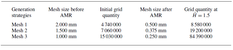
Parameters of different grid generation strategies.

Supplementary movie
Supplementary movie is available at https://doi.org/10.1017/jfm.2025.10422.
Funding
The authors would like to acknowledge support from National Natural Science Foundation of China (grant no.U2441206).
Declaration of interests
The authors report no conflict of interest.
Data availability statement
Source data that support the findings of this study are openly available. The experimental data used to generate figure 26 can be found in the online supplementary materials. All other data that support the plots within this paper and other findings of this study are available from the corresponding author upon reasonable request.
Appendix A. Model validation and grid independence validation
Since this numerical simulation accounts for both the shoulder cavity and the tail cavity, validation of numerical methods for both cavities is required.
We established a vertically constrained underwater launching platform for the ventilated shoulder cavity. Figure 24(a) exhibits the motion and information collection systems of the platform. A motor is used to tow the underwater vehicle along the slide, allowing it to perform single-degree-of-freedom vertical motion. The vacuum pump is used to reduce atmospheric pressure (
 $P_{atm}$
) for the scaled-down experiment. The high-speed camera is placed in front of the observation window to collect the information of the ventilated cavity shape. Moreover, as shown in figure 24(b), gas is delivered to the air seam through a pipeline. The ventilation system consists of an air compressor for gas supply, and a gas control box for ventilation rate regulation. Experimental and numerical simulation conditions are identical:
 $Q=2.8 \times {10^{ - 4}}$
,
 $P_{atm}=6000\,\rm Pa$
. The velocity of the underwater vehicle (
 $u_v$
) in experiment and numerical simulation is shown in figure 25. From
 $T=0$
to
 $0.1\,\rm s$
, the underwater vehicle experiences uniform acceleration, after which it maintains a constant velocity
 $4.1 \,\rm m\,s^{-1}$
. A comparison of experimental and simulated ventilated cavity shapes is presented in figure 26. At
 $T=0.01{-}0.02\,\rm s$
, the velocity of the vehicle is low. After the discharge of non-condensable gas, a ventilated cavity with a large radial size is formed due to the combined effects of the gas’s initial momentum and buoyancy. At
 $T=0.06{-}0.08\,\rm s$
, the end of the ventilated cavity begins to close and develops downstream. At
 $T=0.10{-}0.12\,\rm s$
, the re-entrant jet induces gas–liquid mixing at the ventilated cavity closure, generating the cloudy cavity. Regarding the overall cavity evolution, the experimental and numerical simulation results show strong agreement in the cavity flow patterns. Notably, the numerical model accurately captures special flow patterns, including the cloudy cavity. These findings indicate its effectiveness in simulating ventilated shoulder cavities.
Experimental platform for ventilated cavity. (a) Motion system and information collection system. (b) Ventilation system.

The velocity of the underwater vehicle (
 $u_v$
) in experiment and numerical simulation.

Comparison between the numerical simulation and experimental results of the ventilated shoulder cavity . For more experimental details, please refer to the supplementary material available at https://doi.org/10.1017/jfm.2025.10422.

As for the tail cavity, a comparison is made with the experiment conducted by Cheng et al. (Reference Cheng, Quan, Sha, Yang, Wang and Xu2022b ) at Harbin Institute of Technology HT01 Ventilation Cavity Water Tunnel. As shown in figure 27, a 2 mm diameter nozzle is installed at the bottom of the model, exhausting non-condensable gases at a rate of 30 SLPM. Under the influence of incoming flow with velocity 3 m s–1, a tail cavity is formed. The gas leaks from the end of the tail cavity, forming a twin vortex structure with a long-wavelength ripple. The experimental and numerical results show similar flow patterns. Therefore, it can be concluded that the numerical model can accurately predict the tail cavity.
Comparison between the numerical simulation and experimental results of the tail cavity.

A comparison of cavity shapes under different grid generation strategies.

Grid independence validation is subsequently carried out, and this study employed three different grid generation strategies: mesh 1, mesh 2 and mesh 3. The grid parameters under different grid strategies are shown in table 2. The variation of
 $\bar P_B$
with
 $\bar H$
in case 2 under different grid generation strategies is shown in figure 28. The results shows that the variations of
 $\bar P_B$
are quite similar between mesh 2 and mesh 3, while mesh 1 exhibits significant differences. However, the mesh quantity of mesh 3 is huge and requires a lot of computing resources. Therefore, the current numerical simulation uses the meshing strategy of mesh 2.