1. INTRODUCTION
So-called optically “smoothed” laser beams with speckle structure are characterized by well-known Gaussian statistics for the speckle intensity. Propagation of such beams through an active medium like a warm plasma causes modifications to the speckle statistics, both as a function of time and of space. The extremal statistics of laser speckle fields is of crucial importance to understand the onset of non-linear phenomena in optics and laser–plasma interaction. Speckle patterns of laser fields generated by optical smoothing techniques contain very intense speckles with peak intensities having many times (typically at the order of ten) the mean intensity of the field pattern. Since these smoothing techniques aim to generate Gaussian statistics for the field values (Ceccotti et al., Reference Ceccotti, Bastiani, Giulietti, Biancalana, Chessa, Giulietti and Danson1995), the abundance of intense speckles decreases following an exponentially decreasing law (Rose & DuBois, Reference Rose and Dubois1993a; Garnier, Reference Garnier1999).
The spatial and temporal evolution of laser fields in laser–plasma interaction, or more generally in active media, can change the initial distribution of laser speckles along the propagation through the plasma. The notions of “non-Gaussian” statistics has been evoked in the literature for the high-intensity tail of distribution functions derived from speckle field patterns. The non-linear process responsible for the change in the extreme speckle statistics in laser–plasma interaction are mainly self-focusing (Lushnikov & Vladimirova, Reference Lushnikov and Vladimirova2010) and/or stimulated scattering (mostly stimulated Brillouin forward scattering) (Schmitt & Afeyan, Reference Schmitt and Afeyan1998; Malka et al., Reference Malka, Faure, Hüller, Tikhonchuk, Weber and Amiranoff2003; Grech et al., Reference Grech, Tikhonchuk, Riazuelo and Weber2006; Reference Grech, Riazuelo, Pesme, Weber and Tikhonchuk2009; Depierreux et al., Reference Depierreux, Labaune, Michel, Stenz, Nicolai, Grech, Riazuelo, Weber, Riconda, Tikhonchuk, Loiseau, Borisenko, Nazarov, Hüller, Pesme, Casanova, Limpouch, Meyer, Di-Nicola, Wrobel, Alozy, Romary, Thiell, Soullié, Reverdin and Villette2009).
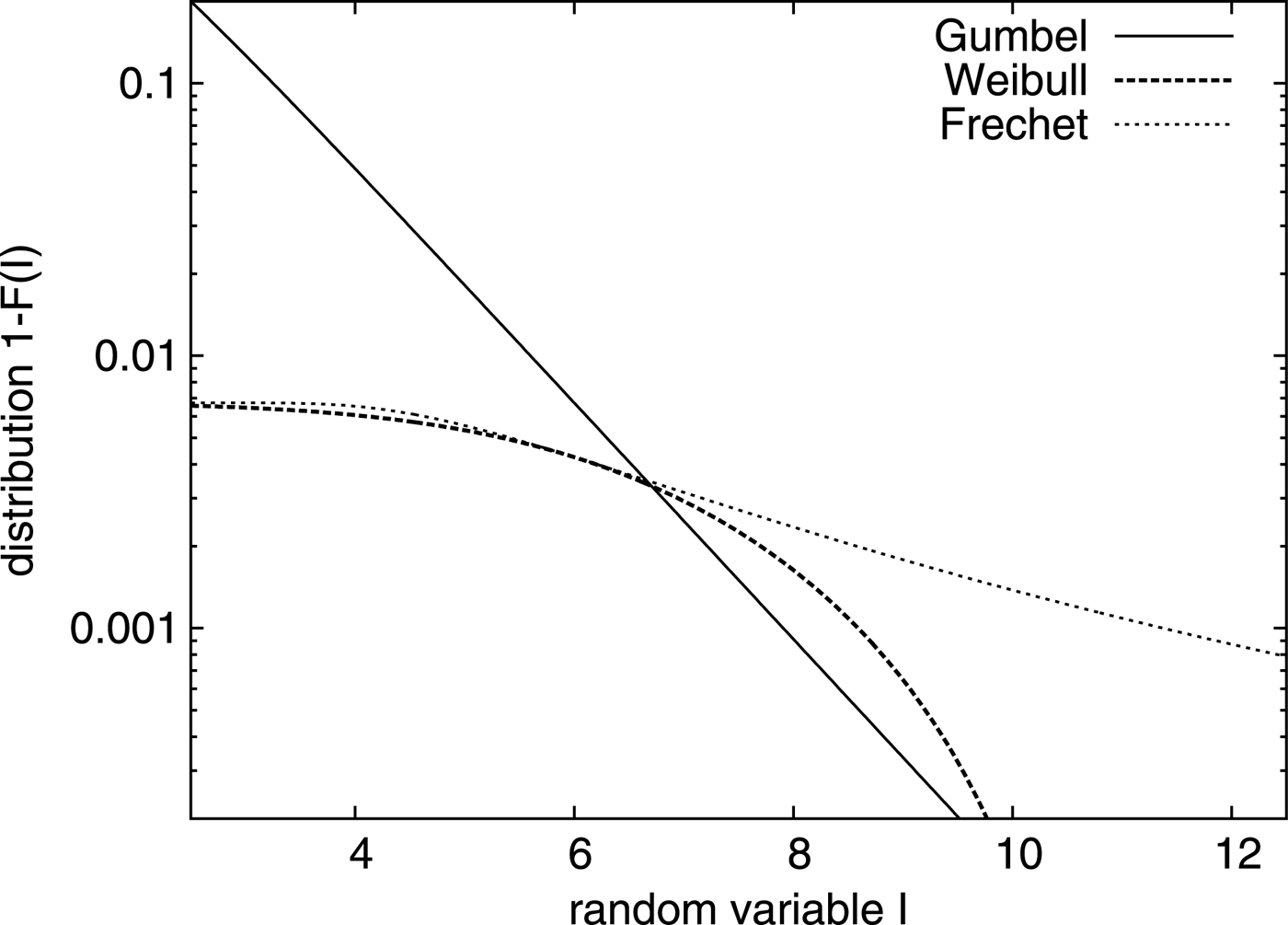
By exploring the functional behavior of the tail of distribution functions, one can distinguish between Gaussian and non-Gaussian statistics. From experimental or numerically determined data, it is however not always evident to conclude which of the three possible types of law of extremal statistics – according to the Fisher–Tippett–Gnedenko theorem (Fisher & Tippett, Reference Fisher and Tippett1928; Gnedenko & Kolmogorov, Reference Gnedenko and Kolmogorov1954) – is the relevant one: The “Gumbel” (or double exponential) law for Gaussian statistics, or the “Weibull” or the “Fréchet” law for non-Gaussian statistics. The extreme value distribution of Fréchet or Weibull type both decrease slowly (as a function of the random variable, here speckle intensity) than a law of exponential-type (“heavy tails” vs. “light”, exponential tails). The so-called “heavy tail” behavior from Lévy statistics, for instance, with a power-law dependence in the tail, belongs to the basin of the Fréchet law, and has been investigated in the context of amplifying random media (Barthélemy et al., Reference Barthelemy, Bertolotti and Wiersma2008; Wiersma, Reference Wiersma2008; Montina et al., Reference Montina, Bortolozzo, Residori and Arecchi2009). To illustrate the allure of the three mentioned extreme value distributions as a function of the random variable, we show the tail behavior in Figure 1.
The three different types of extreme value distributions as a function of the random variable I. The “Gumbel” distribution,  $1 - \exp ( - e^{ - I} )$ (solid line), decreases exponentially ~e −I in the tail for
 $I \gg 1$, while both others have a power-law behavior, “Fréchet” (fine dashed) here ~I −2.5 for all
 $I \gg 1$, and “Weibull” (dashed) here
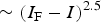 $\sim(I_{\rm F} - I)^{2.5} $ in a finite interval
 $I \to I_{\rm F} $. For detailed explanation see Section 3.1.

In laser–plasma interaction, however, the potential non-linear processes generally saturate with increasing laser intensity. This applies in particular to self-focusing and to stimulated scattering. As we shall see later, due to saturation, heavy tail behavior may be limited to an interval of speckle intensity, and not – like for the above-mentioned cases of Lévy statistics – for the entire tail of the distribution up to the limit of resolution.
Non-linear phenomena, like stimulated scattering usually increase with intensity and can therefore be extremely sensitive to even small changes in the speckle intensity, leading eventually to a critical behavior. Heavy tail behavior due to modified speckle distributions is therefore of particular interest to estimate the risk of increasing deviations (variance) between different realizations, that is, from “shot to shot” in experiments.
For the case of stimulated Raman scattering, Rose and Mounaix (Reference Rose and Mounaix2011) have recently shown evidence for explosive behavior in spite of diffraction. Berger et al. (Reference Berger, Lasinski, Kaiser, Williams, Langdon and Cohen1993) have observed in numerical simulations “hard tail” behavior in the intensity distribution which they attribute to filamentation. Mounaix and Divol (Reference Mounaix and Divol2002) have shown that the cumulative response of Stimulated Brillouin Scattering, based on the independence of speckles (“independent hot spot model”), can spread enormously around a critical gain value associated with the scattering process.
Extremal statistics allows us to examine the probability of events for extreme values of the random variable, here the speckle intensity. The fluctuations between different realizations, around the values indicated by the distribution function, can be more or less important and depend essentially on the type of the limit law. From the order statistics one can determine the probability with which the nth most intense speckle of a pattern with n sp speckles can be found at the intensity I n [hence, I 1 standing for the intensity of the most intense speckle; see, e.g., our previous work (Hüller & Porzio, Reference Hüller and Porzio2010)]. As mentioned earlier, the speckle distribution laws of standard laser smoothing techniques follow Gaussian statistics; the law describing extremal statistics is consequently the Gumbel (double exponential) law. Non-linear phenomena can provoke non-Gaussian statistics due to strong enhancement of the role of speckles at elevated intensity for certain observables, like the total response of the scattered light (Mounaix & Divol, Reference Mounaix and Divol2002; Hüller et al., Reference Hüller, Porzio and Robiche2013), as will be discussed later on. The distribution function associated with this processes appears hence to be “stretched” in the tail, with respect to the linear distribution  $\bar F(I)$, so that the probability to encounter speckles at higher intensities is significantly increased in the interval around I 1, where the intensity I 1 is defined by
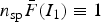 $n_{{\rm sp}} \bar F(I_1 ) \equiv 1$ [i.e.,
 $I \simeq \ln\,n_{{\rm sp}} $, where
 $\bar F\sim\exp \,( - I/\langle I\rangle )$].
In this paper, we show that smoothed laser beams originating from a standard, optical smoothing technique can exhibit a Weibull-type distribution in a limited interval of the speckle peak intensity I, for values of I that are indeed high enough to produce undesirable effects.
The paper is organized as follows: In Section 2, we recall model equations and distributions arising from order statistics. Approximations are deduced to analyze the behavior of densities following the value of the gain G of stimulated scattering inside speckles. A particular analysis is devoted to the Variance in Section 2.2. In Section 3.1, we recall the theoretical basis and the “Excess over Thresholds” methods, which we apply to our model to deduce the nature of the distribution function and its departure from Gaussian statistics. In Section 4, we analyze to which type of limit law belong the speckle distribution functions obtained from our model and from numerical simulations, as a function of the gain parameter of stimulated scattering. Section 5 concludes the paper. Technical computations are presented in an Appendix.
2. MODEL EQUATIONS
In Hüller and Porzio (Reference Hüller and Porzio2010) and Porzio and Hüller (Reference Porzio and Hüller2010), we have derived the probability density in intensity for speckles from order statistics. For the kth speckle in order of its peak intensity I, where k = 11 is the most intense of – in total – n sp speckles, the probability density function (pdf) is given by
 $$f_k (I) = \displaystyle{{n_{{\rm sp}}^k} \over {\Gamma (k)}}e^{ - n_{{\rm sp}} \,e^{ - I} - kI}, $$
where the intensity I is already normalized to the space-averaged intensity of the beam 〈I〉 (here hence  $\langle I\rangle \equiv $ 1). In a subsequent publication (Hüller et al., Reference Hüller, Porzio and Robiche2013), we have shown that in a warm plasma, the speckle statistics is modified by the plasma-induced smoothing (Maximov et al., Reference Maximov, Ourdev, Pesme, Rozmus, Tikhonchuk and Capjack2001) due to the stimulated Brillouin forward scattering (SBFS) process.
2.1. The Non-linear Speckle Distribution and its Probability Density
The SBFS process induces a non-linear modification of the distribution of speckles which can be expressed by taking into account the amplification in the peak intensity of each kth order speckle. In contrast to the linear initial pdf, f k(I), we denote it here as  $f_k^{(G)} (I)$; it is given by
 $$f_k^{(G)} (I) = \displaystyle{1 \over {N_k^{(G)}}} \displaystyle{{n_{{\rm sp}}^k} \over {\Gamma (k)}}e^{G\min (I,I^\ast )} e^{ - n_{{\rm sp}} e^{ - I} - kI}, $$
where G is the standard gain factor for the spatial amplification of stimulated scattering (here forward scattering, SBFS), for an average intensity speckle  $I = \langle I\rangle \equiv 1$ (see Pesme, Reference Pesme, Dautray and Watteau1993; Hüller et al., Reference Hüller, Porzio and Robiche2013); I* stands for the intensity value from which on the stimulated scattering process is saturated; to apply our model properly, saturation should arise for speckles having at least several times the average intensity, that is, I* > 2. As saturation process we assume here pump depletion, which means that the scattering, starting from the seed level
 ${\rm \varepsilon} _{{\rm seed}} $, cannot be amplified beyond the level of the “pump” wave intensity, that is,
 ${\rm \varepsilon} _{{\rm seed}} \exp \,(GI) \le {\rm \varepsilon} _{{\rm seed}} \exp \,(GI^\ast ) \equiv 1$. The normalization
 $N_k^{(G)} $ in Eq. (1) of the pdf is given by
 $N_k^{(G)} = \int_0^\infty {(n_{{\rm sp}}^k /\Gamma (k))} e^{G\min (I,I^\ast )} e^{ - n_{{\rm sp}} \exp ( - I) - kI} dI$.
The gain value G of SBFS for the average (beam and speckle) intensity I 15 in units of 1015 W/cm2 at the laser wavelength λμm in microns and at electron temperature T e in keV, can be estimated as  $G \lesssim ({\rm \pi }/2){({\rm \omega }/\nu )_{{\rm iaw}}}(n/{n_c})(0.1\;{I_{15}}{\rm \lambda }_{{\rm \mu m}}^2 /{T_{{\rm e,keV}}})\ell ({\rm \theta })$, (Hüller et al., Reference Hüller, Porzio and Robiche2013) with
 $({\rm \omega} /\nu )_{{\rm iaw}} $ standing for the ratio between frequency and damping of the ion acoustic wave, n/n c the ratio between electron density and critical density, and
 $\ell ({\rm \theta} ) \simeq f_\# [\sqrt {\rm \pi} /2\cos ({\rm \theta} /2)],$ where f # is the speckle f-number and
 $0 \lt {\rm \theta} \lt {\rm \pi} /2$ the scattering angle with respect to the laser propagation.
Numerical simulations of plasma-induced smoothing clearly confirm the features of this distribution, so that we use the distribution for further evaluation and to analyze it with respect to its maximum domain of attraction (MDA) (see paragraph 4).
In the following, we work out simplified expressions for the probability density f (G)(I) corresponding to the complementary distribution (also named tail distribution) function  $\bar F^{(G)} (I)$, defined as
 $$\bar F^{(G)} (I) = 1 - F^{(G)} (I) = n_{{\rm sp}}^{ - 1} \sum\limits_k^{n_{{\rm sp}}} {\int_I^\infty {\,f_{\rm k}^{(G)}}} (I^{\prime})dI^{\prime}.$$
This function represents the complementary distribution sufficiently well at least for  $I \gg $ 1 (in practice I > 4). In order to derive the pdf of the non-linear distribution we will make use of the well-known identities for the diverse types of gamma functions, which will be needed for the following expressions:
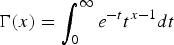 $\Gamma (x) = \int_0^\infty {e^{ - t}} t^{x - 1} dt$,
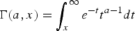 $\Gamma (a,x) = \int_x^\infty {e^{ - t}} t^{a - 1} dt$,
 ${\rm \gamma} (a,x) = \int_0^x {e^{ - t}} t^{a - 1} dt = \sum\nolimits_{n = 0}^\infty {( - 1)^n} x^{a + n} /[n!(a + n)]$, and
 $\Gamma (a,x) = \Gamma (a,0) - {\rm \gamma} (a,x) = \Gamma (a) - {\rm \gamma} (a,x)$, and for the k integer
 ${\rm \gamma} (k,x) = (k - 1)!\left( {1 - e^{ - x} \sum\nolimits_{n = 0}^{k - 1} {x^n} /n!} \right)$.
The probability density f (G)(I) as well as the distribution f (G)(I), following Eq. (2), can then be expressed as follows:
 $$f^{(G)} (I) = e^{ - n_{\rm sp} e^{ - I}} e^{G\min ({\rm I},{\rm I}^{\ast})} \sum\limits_{k = 1}^{n_{\rm sp}} \displaystyle{e^{ - kI} n_{\rm sp}^k \over D_k (G,0)}, $$
 $$\eqalign{\bar F^{(G)} (I) & = \sum\limits_{k = 1}^{n_{{\rm sp}}} {\displaystyle{{D_k (G,I)} \over {D_k (G,0)}}} \cr & \equiv \sum\limits_{k = 1}^{n_{{\rm sp}}} {\displaystyle{{n_{{\rm sp}}^k} \over {D_k (G,0)}}} \int_I^\infty dI^{\prime}e^{ - n_{{\rm sp}} e^{ - I^{\prime}}} e^{ - kI^{\prime} + G\min (I^{\prime},I^\ast )}, }$$
with
 $$\eqalign{&D_k (G,I) \equiv \cr &\left\{\matrix{n_{\rm sp}^G \left[\Gamma (k - G,n_{\rm sp} e^{ - I^{\ast}}) - \Gamma (k - G,n_{\rm sp} e^{ - I}) \right] \cr + e^{GI^{\rm \ast}} {\rm \gamma} (k,n_{\rm sp} e^{ - I^{\ast}}\!\!\!\!\!),\quad {\rm for} I \lt I^{\ast} \hfill \cr {} \hfill \cr e^{GI^{\ast}} {\rm \gamma} (k,n_{\rm sp} e^{ - I}), {\rm for} I \ge I^{\ast}. \hfill} \right.}$$
Note that the normalizing denominator D k(G, 0) yields D k(G = 0, 0)= ${\rm \gamma} (k,n_{{\rm sp}} e^{ - I} )$ for the linear case G = 0. In order to understand the non-linear modification of the pdf f (G) and the distribution F (G), it is instructive to develop Eqs. (3) and (4) for the particular cases G = 1/2 and 3/2 (see the Appendix), and for cases with integer values of the gain G, namely
 $$f^{(G)} (I) \equiv f_a^{(G)} (I) + f_b^{(G)} (I),\ {\rm for}\;G \in {\open N}$$
 $$ \simeq {e^{ - {n_{{\rm sp}}}{e^{ - I}}}}{e^{G\min (I{\rm ,}{I^\ast})}}\left( {\sum\limits_{k = 1}^{G} {\displaystyle{{{e^{ - kI}}n_{{\rm sp}}^k } \over {{D_k}(G,0)}}} + {n_{{\rm sp}}}{e^{ - (G + 1)I}}{e_{{n_{{\rm sp}}} - G - 1}}({n_{{\rm sp}}}{e^{ - I}})} \right),$$
with  $e_n (x) = \exp (x)\Gamma (n + 1,x)/n!$ which approaches
 $e_n (x)\sim \exp (x)$ for
 $n \gg x$. In the intensity interval I < I*, that is, before saturation of amplification, the term
 $f_b^{(G)} (I) = n_{{\rm sp}} e^{ - I - n_{{\rm sp}} e^{ - I}} e_{n_{{\rm sp}} - G - 1} (n_{{\rm sp}} e^{ - I} )$ is practically independent of G, except for the missing terms of the first (i.e., the most intense) maxima. For the complementary distribution
 $\bar F^{(G)} $, the same holds for the part
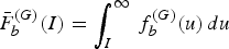 $\bar F_b^{(G)} (I) = \int_I^\infty {\,f_b^{{\rm (}G{\rm )}}} (u)\,du$, being well approximated by
 $\bar F_b^{(G)} (I) \simeq \exp ( - I)$ for I* > I > 1,
 $$\eqalign{\bar F^{(G)} (I) & \equiv \bar F_a^{(G)} (I) + \bar F_b^{(G)} (I) \simeq \sum\limits_{k = 1}^{G \in {\open N}} {\displaystyle{{D_k (G,I)} \over {D_k (G,0)}}} \cr & \quad+ e^{ - I}, \quad {\rm for}\;G \in {\open N}.}$$
For I > I*, the contribution  $\bar F_b^{(G)} (I)$ has a faster, but still exponential decrease, and can be neglected with respect to
 $\bar F_a^{(G)} (I)$. The terms
 $f_a^{(G)} (I) = \sum\nolimits_{k = 1}^G {( \cdots )} $ and
 $\bar F_a^{(G)} (I) = \sum\nolimits_{k{\rm = 1}}^G {{\rm D}_k} (G,I)/D_k (G,0)$, for which the speckle order k (intensity decrease with order) is less or equal G, k ≤ G, constitute, hence the non-linear part of the pdf and the distribution, respectively, due to an enhancement of the probability to find the most intense speckles at still higher intensity. The complementary distribution F (G)(I) is “stretched” in the high-intensity tail, that is, the probability to find intense speckles at intensities higher than in absence of the plasma is considerably increased for
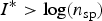 $I^\ast \gt \log (n_{{\rm sp}} )$, and F (G)(I) therefore exhibits clearly a non-exponential decrease, as illustrated in Figure 1. As can be observed in the figures, there is a drastic change in the functional behavior of distributions between the domains G < 1 ≤ k and G ≥ k ≥ 1.
In the Appendix, we also develop approximate expressions for F (G)(I), for cases of the gain coefficient G with half-integer values, such as G = 1/2, 3/2 (Fig. 2).
Complementary speckle distribution  $\bar F^{(G)} (I)$ in the high-intensity tail. The total number of speckles considered here is n sp = 2300, so that the most intense speckles has its expectation value at
 $I_1 /\langle I\rangle = \log (2300) + \gamma _{\rm E} \simeq 8.3$. The onset of saturation is at I* = 11 here. Subplot (a) shows the cases G = 1/2 (green line), 1 (blue), 3/2 (red), and 2 (yellow-green). Subplot (b) shows only the cases G = 1 and 3/2, but distinguishes contribution from all speckles (blue and red lines, respectively), and from the most intense speckles
 $\bar F_a^{(G)} $ (yellow and green lines, respectively).
2.2. Variance
Although the number of speckles in the high-intensity tail of the distribution is small, the impact of a modified distribution function on physical observables in the regime around and above the critical gain G = 1 is important. Moreover, the fluctuations between different realizations of speckle patterns will be particularly pronounced. For this reason we also calculate here moments to the pdf of the modified speckle distribution, and compute the variance of the speckle intensity which is an important measure to estimate the differences arising in different realizations of speckle patterns governed by the distribution FG(I). Our results in Hüller et al. (Reference Hüller, Porzio and Robiche2013) show that in particular for gain values G close to the critical value G = 1 the variance can be surprisingly high.
In order to evaluate moments of the pdf it is easier to perform a change of variables by replacing the variables n sp, I, and I*, by  $x = n_{{\rm sp}} \;e^{ - I} $, and
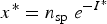 $x^\ast = n_{{\rm sp}} \;e^{ - I^\ast} $, as we have done in the Appendix. The approximate expression of the pdf for
 $f^{({\rm G})} (I) \to \tilde f^{({\rm G})} (x)$ then reads
 $$\eqalign{{\tilde f}^{(G)} (x) & = e^{-x} \left(n^G \sum\limits_{k = 1}^{G - 1} \displaystyle{x^{k - G} \over D_k (G,0)} + \displaystyle{n^G \over D_{k = G} (G,0)} + x e_{n - G - 1} (x) \right), \cr & \!\!\quad \quad {\rm for}\;x \gt x^{\ast}, \quad {\rm i.e.}\;I^{\ast} \gt I, \cr & = e^{-x} \left( \left(\displaystyle{n \over x^{\ast}} \right)^G \sum\limits_{k = 1}^{G - 1} \displaystyle{x^k \over D_k (G,0)} + \displaystyle{n^G (x/x^{\ast})^G \over D_{k = G}(G,0)}\right. \cr &\quad \quad \left. + x \left(\displaystyle{x \over x^{\ast}} \right)^G e_{n - G - 1} (x) \right), \qquad{\rm for}\;x \lt x^{\ast}.}$$
The expression written in this form distinguishes between three contributions: The sum term, over  $k = 1, \ldots, G - 1$, of the first contribution contains the peak term(s) (only if G > 1), the second one is the contribution for G = 1 only, and corresponds to a plateau-like behavior as a function of intensity I, while the third contribution is essentially of linear nature and decreases in intensity I. This third contribution as expressed here, since it was derived from order statistics, is only valid for large enough speckles intensities, say I > 3. It overestimates the pdf in the low-intensity part.
Consequently, only the two first contributions alter the momenta of the distribution for different values of the gain G. They primarily contribute to the change in the variance as a function of G. For the interval x < x* (or I > I*) all the terms have powers of  $x/x^\ast \lt 1$, and therefore are rapidly decreasing.
From the pdf we determine the variance, Var(I) in I to the expectation value  $\langle I\rangle \equiv E(I)$ of the speckles,
 ${\rm Var}(I) = E(I^2 ) - E(I)^2 $, via an approximate calculation, keeping only the dominating (i.e., peak and plateau) term(s). By definition, the second moment of a pdf of I is given, in our notation, by
 $$E(I^2) = \int_0^{\infty} I^2 f^{(G)} (I)dI = \int_0^n \left(\log \displaystyle{n \over x} \right)^2 \tilde f^{(G)} (x)\displaystyle{dx \over x}.$$
Taking for the probability density  $\tilde f^{(G)} (x)$ for even integer values of G, the peak term in the above sum is reached for k = G/2, and for odd integer G, two equal peak terms, for k = [G/2] and k = [G/2] + 1 have to be considered.
Hence, for most interesting case G = 1, one obtains with the leading term,
 $$E(I^2 ) \vert _{G = 1} \simeq \int_{ne^{ - {\rm I}^\ast}} ^n {\left( {\log \displaystyle{n \over x}} \right)^2} \displaystyle{{ne^{ - x}} \over {D_{k = 1} (G = 1,0)}}\displaystyle{{dx} \over x}.$$
An approximate expression for the variance with G = 1 is hence given by
 $$\eqalign{{\rm Var} \vert _{G = 1} (I) & = \int_{ne^{ - I^\ast}} ^n {\left( {\log \displaystyle{n \over x}} \right)^2} \displaystyle{{ne^{ - x}} \over {D_{k = 1} (G = 1,0)}}\displaystyle{{dx} \over x} \cr & \quad- \left( {\int_{ne^{ - I^\ast}} ^n {\log} \displaystyle{n \over x}{\rm} \displaystyle{{ne^{ - x}} \over {D_{k = 1} (G = 1,0)}}\displaystyle{{dx} \over x}} \right)^2,}$$
involving three integrals  $\int {x^{ - 1}} e^{ - x} dx$,
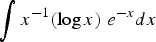 $\int {x^{ - 1}} (\log x)\;e^{ - x} dx$, and
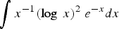 $\int {x^{ - 1}} (\log \;x)^2 \;e^{ - x} dx$, which can be expressed in terms of the Γ(a, x) function and its derivatives:
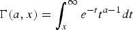 $\Gamma (a,x) = \int_x^\infty {e^{ - t}} t^{a - 1} {\mkern 1mu} dt$,
 $\partial _a \Gamma (a,x) = \int_x^\infty {e^{ - t}} t^{a - 1} \log \;t{\mkern 1mu} dt$, and
 $\partial _a^2 \Gamma (a,x) = \int_x^\infty {e^{ - t}} t^{a - 1} (\log \;t)^2 {\mkern 1mu} dt$.
Based on our model, we have determined the variance Var(G) for two parameters sets, namely with n sp = 2300 and I* = 11 as well as n sp = 3000 and I = 15 showing the increase of the variance as a function of the gain G in the interval 0 ≤ G ≤ 2.5 due to the increasing peak value of the most intense speckles (Fig. 3).
The increase in the variance with G is due to the contributions of the leading terms, as discussed above, that is, due to the most intense speckles. The expectation value (in peak intensity) of the most intense speckles grows rapidly with G, so that already few intense speckles can raise the variance significantly.
3. HOW TO DETERMINE THE TYPE OF STATISTICS
The “non-linear” speckle distribution and its density derived in Eqs. (3 and 4) on the basis of order statistics, for a laser speckle pattern under the influence of stimulated scattering, follow our preceding work (Hüller et al., Reference Hüller, Porzio and Robiche2013), Eqs. (31) and (33), in which we also have presented simulation results supporting the model results. Both the distribution from the model and the simulations show a clear departure from an exponential decrease in the high-intensity tail, for G ≥ 1. This behavior can be observed in a limited interval in the vicinity of the expectation value of the speckle peak intensity  $I_1 \simeq \log (n_{{\rm sp}} ) + {\rm \gamma} _{{\rm Euler}} \;({\rm \gamma} _{{\rm Euler}} = 0.5772$).
While a power-law-like behavior in the tail of complementary distributions is a clear signature of non-Gaussian statistics, it has still to be distinguished between the two types of non-Gaussian limit laws of the extremal behavior, namely the Weibull or Fréchet laws (Wiersma, Reference Wiersma2008; Montina et al., Reference Montina, Bortolozzo, Residori and Arecchi2009).
The distinction between the different limit laws needs careful analysis of the data for which, however, mathematical methods have been derived allowing us to determine the correct type.
For distributions for which a power-law behavior fits in the tail up to the highest measurable value of the variable (here, the intensity) it is plausible to identify the Fréchet law as limit law (Wiersma, Reference Wiersma2008; Montina et al., Reference Montina, Bortolozzo, Residori and Arecchi2009). In cases, however, when the distribution exhibits non-exponential behavior only in a limited interval, like the case shown in Figure 1, computed from our model, the distribution has to be carefully determined, in particular the lower bound of the relevant interval.
For this reason, we examine here the character of the distribution functions on the basis of well-established theory (Pickands, Reference Pickands1975; Leadbetter, Reference Leadbetter1991; Embrechts et al., Reference Embrechts, Klüppelberg and Mikosch1997).
A good method to plausibly demonstrate the type of statistics is to determine the behavior by fitting “excesses over a threshold” (Embrechts et al., Reference Embrechts, Klüppelberg and Mikosch1997). This is done on the basis of the generalized Pareto distribution (GPD) for the conditioned distribution function  $\bar F_{{\rm th}} (y)$ evaluated at the “threshold” (“th”) speckle intensity I th that has to be suitably chosen. Then, once the type of Pareto distribution for the conditioned F th is known, it is possible to deduce the nature of the underlying distribution F.
3.1. Excess Over Threshold and Limit Theorems
For the distribution function F(I), with  $\bar F \equiv 1 - F$ denoting the complementary distribution function, we determine the “excess over threshold” probability
 $\bar F_{{\rm th}} (y)$. This conditional probability is the probability
 $P(I \gt I_{{\rm th}} + y)$ that the speckle intensity I is larger than the value I th + y knowing that I is larger than the threshold intensity I th, that is,
 $P(I \gt I_{{\rm th}} )$. As a function of the distribution
 $\bar F$ and for
 $y \in {\open R}^ + $, it can be expressed as
 $$\bar F_{{\rm th}} (y) \equiv \displaystyle{{P(I \gt I_{{\rm th}} + y)} \over {P(I \gt I_{{\rm th}} )}} = \displaystyle{{\bar F(I_{{\rm th}} + y)} \over {\bar F(I_{{\rm th}} )}}.$$
It has been shown in Pickands (Reference Pickands1975), Balkema and DeHaan (Reference Balkema and De Haan1974), Leadbetter, Reference Leadbetter1991 and in the review of Embrechts et al. (Reference Embrechts, Klüppelberg and Mikosch1997), that for a suitably chosen large threshold value I th, the conditional distribution F th tends toward h a,c the “GPD” (see below) if and only if the (unconditioned) distribution F(I) is in the maximal domain of attraction of “the generalized extreme value distribution” H c, with the same parameter c:
 $$H_c (y) = \left\{ {\matrix{ {\exp \{ - (1 + cy)^{ - 1/c} \}, \quad {\rm for}\;c \ne 0} \hfill \cr {\exp \{ - e^{ - y} \}, \quad {\rm otherwise},\;{\rm i}{\rm. e}.,\;c = 0,} \hfill \cr}} \right.$$
requiring y > 1/c if c > 0, and  $y \lt - 1/c$ if c < 0; for the case c = 0 with
 $y \in {\open R}$ this yields the Gumbel (limit) law, which corresponds to Gaussian statistics.
The three corresponding cases for the GPD h a,c with a > 0 following the value of  $c \in {\open R}$, are:
 $$h_{c{\rm,} a} (y) = \left\{ {\matrix{ {\left( {1 + c\displaystyle{y \over a}} \right)^{ - 1/c} \quad \,\,\,{\rm for}\;c \gt 0\quad {\rm and}\;y \lt \infty,} \hfill \cr {\;e^{ - y/a} \qquad\ \ \qquad{\rm for}\;c = 0\quad {\rm and}\;y \lt \infty,} \hfill \cr {\left( {1 - \vert c \vert \displaystyle{y \over a}} \right)^{1/ \vert c \vert} \quad {\rm for}\;c \lt 0\quad {\rm and}\;0 \lt y \le \displaystyle{a \over { \vert c \vert}}.} \hfill \cr}} \right.$$
In our case, following Pickands (Reference Pickands1975), we find that  $\bar F_{{\rm th}} (y)$ can be given in very good approximation by h c,a with c < 0, so that F belongs to the extreme value attraction basin of a Weibull law with the same value c < 0. It is important to remark in this case that for
 $y \gt a/\vert c \vert$, h c,a is no longer defined, and the conditioned probability
 $\bar F_{{\rm th}} (y \gt a/\vert c \vert) = 0$. Therefore, the interval for a Weibull-type distribution is limited. Physically this is due to the fact that the non-linear process that leads to our distribution F(I) saturates in I, and therefore the interval is limited in I where the Weibull distribution applies.
For distributions that can be described with such a type of functions for the case c < 0, a particular property is that, approaching a certain finite value  $y_{\rm F} = \vert a/c \vert \lt \infty $ of the variable y (in our case the speckle intensity above I th), the (unconditioned) distribution has a power-law dependence in the vicinity of
 $I\,\sim\,I_{\rm F} \equiv I_{{\rm th}} + y_{\rm F} $. This feature can be expressed, via the distribution function F(I) and its corresponding probability density
 $f\,(I) = F^{\prime}(I)$, as
 $$\mathop {\lim} \limits_{\matrix{ {I \to I_{\rm F}} \cr {I \lt I_{\rm F}} \cr}} \displaystyle{{(I_{\rm F} - I)f\,(I)} \over {\bar F(I)}} \to {\rm \alpha}, $$
with  $I_{\rm F} = I_{{\rm th}} + y_{\rm F} $, and with f(I) being the probability density belonging to
 $\bar F(I)$, hence
 $f^{(G)} (I) \equiv dF^{(G)} (I)/dI$ in our particular case. The upper bound of the interval at y = y F marks the end point of the theoretical distribution,
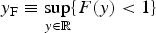 $y_{\rm F} \equiv \mathop {\sup} \limits_{y \in {\open R}} \{ F(y) \lt 1\} $, namely the value in y where the conditioned distribution F th
 $(= 1 - \bar F_{{\rm th}} $) reaches
 $F_{{\rm th}} (y = y_{\rm F} ) \equiv 1$ (or
 $\bar F_{{\rm th}} (y_{\rm F} ) = 0$).
Distributions resulting from the GPD method with negative c are hence associated with Weibull distributions. In a neighborhood of  $I = I_{{\rm th}} + y_{\rm F} $, for
 $I \to I_{\rm F} $, I < I F [see Embrechts et al. (Reference Embrechts, Klüppelberg and Mikosch1997, 152–154) the unconditioned distribution F belongs to the corresponding MDA of the Weibull law Ψα,
 $$\Psi _{\rm \alpha} (I) = e^{ - ( - I)^{\rm \alpha}}, $$
which is qualitatively different from the domain of attraction of the Gumbel law,  $\sim\!\!\exp ( - e^{ - I} )$, to which exponential type distributions from Gaussian statistics belong. From the limit theory, it follows that the power law with an exponent α can be established in the vicinity of I = I F, but only in the branch
 $I \to I_{\rm F} $, I < I F, namely
 $$\bar F(I) \simeq K(I_{\rm F} - I)^{\rm \alpha}, \quad {\rm for}\;I_{\rm F} \gt I \gt I_{\rm F} - K^{ - 1/{\rm \alpha}}, $$
in which the coefficient K is related the lower bound of the interval of validity of this approximation, namely  $I \gt I_{\rm F} - K^{ - 1/{\rm \alpha}} $. The exponents of the GPD in Eq. (11), for the case c < 0, and of the limit law Eq. (13) are linked (Embrechts et al., Reference Embrechts, Klüppelberg and Mikosch1997); in the ideal limit case, this would yield
 ${\rm \alpha} = - 1/c$.
In the following, we will evaluate the coefficients c, a in Eq. (11) and K and α in Eq. (14) from the distribution of Eq. (4).
4. RESULTS
We have hence examined the distributions following our model, Eq. (4) for different values of the gain parameter G, namely for G = 1, 1.5, 2, and for G = 0.5 < 1. Following what has been explained in the previous paragraph, two approaches can be used to find fits to power laws according to the observed features, using
(i) the GPD from “excess over threshold” theory, Eq. (11), or
(ii) to directly seek for a fit to Eq. (14).
Examining Figure 1 graphically, one can observe exponential decrease of the distribution in the low-intensity and the very high-intensity tail as a function of I. In between both exponential regimes the distribution is obviously non-exponential, but it is not evident to clearly identify where the transition toward the high-intensity tail takes place. Therefore, approach (ii) is not the first choice, but can be used once the coefficient found from approach (i) have been determined. One would use I th and y F (if existing) from (i) and seek for the power exponent α in Eq. (14), and eventually verify the equivalence between the respective coefficients as discussed in Section 3.1.
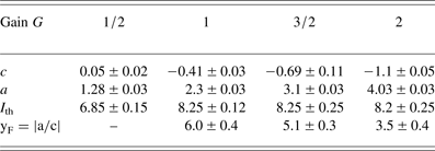
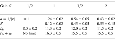
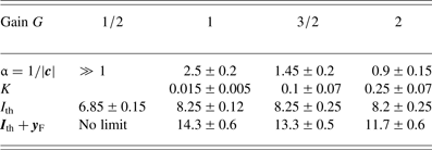
For two sets of the parameters n sp and I*, we have computed the distribution function and determined the coefficients using approach (i). The results are displayed in Tables 1–4.
Summary of the parameters for the GPD fit as a function of gain values G for n sp = 3000 and I* = 15
Summary of the parameters for the GPD fit as a function of gain values G for n sp = 2300 and I* = 11
Summary of parameters of the Weibull-type power law valid in the limit  ${\rm I}_{{th}} \le {\rm I} \lt {\rm I}_{F} = {\rm I}_{{th}} + y_{F} $. Here n sp = 3000 and I* = 15, corresponding to Table 1
Summary of parameters of the Weibull-type power law valid in the limit  ${\rm I}_{{th}} \le {\rm I} \lt {\rm I}_{F} = {\rm I}_{{th}} + y_{\rm F} $. Here n sp = 2300 and I* = 11 corresponding to Table 2
We have first determined the conditioned distribution  $\bar F_{{\rm th}} $ by varying the threshold intensity I th and seeking for convergence in the values of c and a of the fit to the function h c,a(y) of Eq. (11). The value of I th can be assumed to be in the vicinity of log n sp and has to be chosen as I th < I* (since otherwise non-linear effects will already be saturated).
Pickands (Reference Pickands1975) suggests a method to determine the value of c based on specific quantile values of  $\bar F_{{\rm th}} (y)$, namely by determining the values y 1 and y 2, where
 $\bar F_{{\rm th}} (y_1 ) = $ 50% and
 $\bar F_{{\rm th}} (y_2 ) = $ 25% such that
 $c = \log (y_2 /y_1 - 1)/\log (2)$.
Numerical algorithms allow, however, to more reliably find the values of c and a by searching the best fit of h c,a(y) to  $\bar F_{{\rm th}} (y)$. This is what we have done to obtain the values in Tables 1 and 2. The fit to
 $\bar F_{{\rm th}} (y) = 1 - F_{{\rm th}} (y)$ is shown in Figure 4 for the particular case G = 3/2, n sp = 3000 (or
 $\log n_{{\rm sp}} \simeq 8$), and I* = 15. The values for c and α are stable with respect to the choice of the threshold value in the vicinity of
 $I_{{\rm th}} \sim10 \pm 1$ at least, being close to the expectation value
 $I_1 = \log n_{{\rm sp}} + 0.5772$ of the peak intensity of the most intense speckle [determined from order statistics, Hüller and Porzio (Reference Hüller and Porzio2010)].
Comparison between the complementary “excess over threshold” distribution function  $\bar F_{{\rm th}} = 1 - F_{{\rm th}} $ deduced from our model, Eq. (2), the GPD, following Eq. (11),
 $(1 - \vert c \vert y/a)^{1/\vert c \vert} $, and the power-law expression
 $K(y_{\rm F} - y)^{\rm \alpha} $ with
 $y_{\rm F} = a/\vert c \vert$, for the case G = 3/2, with
 $c = \simeq $ −1.8, a = 8.,
 $y_{\rm F} \simeq 4.4$, K = 0.45, and α = 0.53.
The width of the intensity interval corresponding to a Weibull law is given by  $y_{\rm F} = \vert a/c \vert$ if c < 0, so that a Weibull-type distribution is found in
 $I_{{\rm th}} \lesssim I \lt I_{\rm F} = I_{{\rm th}} + y_{\rm F} $. The values found here (
 $I\,\gtrsim\;{I_{{\rm th}}}$) are great enough to reasonably guarantee convergence toward the Weibull law.
The results show a clear distinction between the case G = 0.5 < 1 and the other cases with G ≥ 1: For G = 0.5, the value of c is very small so that the behavior, as a function of the excess parameter y, is not significantly departing from an exponential decrease, while there is a clear non-exponential behavior for G ≥ 1 in the interval y F > y > 0. For the function h c,a of the GPD a finite upper limit of this interval exists due to negative value of c, simply due to the fact that otherwise the probability for y > y F would exceed 100%. The tail of the conditioned distribution  $\bar F_{{\rm th}} $ shows a smooth decrease for y ~ y F, instead of an abrupt behavior of h c,a at y F, corresponding to the end of validity of the Weibull law. Beyond y F (or
 $I \gtrsim I_{\rm F} \gt $) the distribution is again of exponential type because of the onset of saturation.
We observe a clear and systematic decrease of the coefficient c with the gain value G, starting from a small value  $\vert c \vert \ll $ 1 for G < 11. As exposed in the previous paragraph, it follows that the exponent of the power-law behavior corresponding to Eq. (14), namely
 ${\rm \alpha} = - 1/c$, hence decreases with increasing G, explaining a flattening of the distribution
 $\bar F(I)$ in the interval
 $I_{\rm th}\,\lesssim\,I \lt {I_{\rm F}}$. Both the flattening and the great enough intensity values imply the onset of a heavy tail distribution function which has to be seen as a “caveat” for extremal statistics, eventually causing undesirable effects.
In addition to the method with approach (i), where we determined the coefficients to the function Eq. (11) via fitting to the conditioned distribution  $\bar F_{{\rm th}} $, we have also directly analyzed the distributions
 $\bar F(I)$ – computed from Eq. (4) for the different G-values – with respect to the power law of Eq. (14). As input to obtain a best fit, we have used the values of
 $I_{\rm F} = I_{{\rm th}} + y_{\rm F} $ from Tables 1 and 2. The results of the fit for the coefficients α and K are listed in Tables 3 and 4.
The values determined via both approaches – that is, approach (i) with the GPD method with Eq. (11) and via approach (ii) using the power-law expression Eq. (14) – prove to be consistent, in particular what concerns the interval where the Weibull-type distribution has to be considered.
For the interval  $I \lt I_{\rm F} - K^{ - 1/{\rm \alpha}} $ the distribution keeps the characteristics of an exponential distribution, meaning that smaller intensity speckles still obey Gaussian statistics. The consistency with the power-law dependence in a limited interval is also illustrated graphically in Figures 4–7. In Figure 4, the power-law according to the function Eq. (11) is directly compared with the conditioned complementary distribution
 $\bar F_{{\rm th}} $ for the example case with G = 3/2, in Figure 5, for the same case, we show the comparison between the complementary speckle distribution
 $\bar F(I)$ and the power law deduced via the GPD in a linear scale, while in Figures 6 and 7 the comparison between the computed complementary distributions and the power law according to Eq. (14) is depicted in log scale for G = 1, 3/2, and 2. One can see that the values for each
 $\bar F_{{\rm th}} $ fit very well to the power-law curves
 $\sim K(I_{\rm F} - I)^{\rm \alpha} $ for the values and intervals indicated in Tables 3 and 4.
Illustration of non-exponential behavior of the complementary distribution  $\bar F(I) = 1 - F(I)$ [from our model Eq. (2)] in the interval between I = I th (y = 0, top axis) and
 $I \equiv I_{\rm F} = I_{{\rm th}} + y_{\rm F} $ (y = y F, top axis) where the behavior can be approximated by a power-law-type function
 $K(y_{\rm F} - y)^{\rm \alpha} $ deduced from a GPD. Shown is the case of G = 3/2 with
 $y_{\rm F} \simeq 4.4$,
 ${\rm \alpha} \simeq 0.53$, and
 $K \simeq 0.45$, consistent with the parameters
 $c \simeq - 1.8$,
 $a \simeq 8$ from the GPD.
Complementary speckle distribution  $\bar F^{({\rm G})} (I)$ [multiplied by n sp in the high-intensity tail for the gain values G = 1 (blue line), 3/2 (red), and 2 (yellow-green)] and the power laws deduced with the help of the GPD, and taken from Table 4, that is, G = 1: α = 2.3, I F = 13.7; G = 3/2: α = 1.45 and I F = 13; and G = 2: α = 0.85 and I F = 11.6. Solid lines: Model; dashed lines: Power law following Eq. (14). The total number of speckles considered here is n sp = 2300. The onset of saturation is set to I* = 11 here.
Complementary speckle distribution  $\bar F^{(G)} (I)$ [multiplied by n sp] in the high-intensity tail for the gain values G = 1 (blue line), 3/2 (red), and 2 (yellow-green) and the power laws deduced with the help of the GPD, and taken from Table 3, that is, G = 1: α = 0.8, I F = 16.4; solid lines: Model; dashed lines; power law following Eq. (14); G = 3/2: α = 0.54 and I F = 15.5; and G = 2: α = 0.43 and I F = 15.4. Parameters n sp = 3000 and I* = 15 here.
As in Hüller et al. (Reference Hüller, Porzio and Robiche2013) we have performed two-dimensional (2D) simulations with the code Harmony2D (Hüller et al., Reference Hüller, Masson-Laborde, Pesme, Casanova, Detering and Maximov2006; Reference Hüller, Porzio and Robiche2013) for the same parameters as in the computation of  $\bar F_{{\rm th}} $ from Eq. (4) for n sp = 2300, I* = 11, and for G = 1 and 3/2. The distributions are determined from snapshots from the speckle field pattern taken from a plasma layer of approximately 2.5 times a speckle length, as explained in Hüller et al. (Reference Hüller, Porzio and Robiche2013). The simulation results (see Figs. 8 and 9) show very good agreement both with the computation using
 $\bar F_{{\rm th}} $ from Eq. (4). Evidently, also the Weibull-type power-law behavior can be observed in the same speckle intensity interval.
For the case G = 1: Comparison between the complementary distribution of speckles obtained from simulations of forward SBS [as in Hüller et al. (Reference Hüller, Porzio and Robiche2013)], the power-law dependence  $\bar F \propto (I_{\rm F} - I)^{\rm \alpha} $, and the model following Eq. (4). The power-law dependence determined via the GPD is valid in the limited interval
 $I_{\rm th} \lesssim \,I \lt {I_{\rm F}}$, with
 $I_{\rm F} \simeq 12.2$,
 $I_{{\rm th}} \simeq 8$, and
 ${\rm \alpha} \simeq 2.25, \ldots, 2.45$. The total number of speckles in the simulations was
 $n_{{\rm sp}} = 2300$.
As in Figure 8, but for G = 1.5: Comparison between the complementary distribution of speckles obtained from simulations of forward SBS, the power-law dependence  $\bar F \propto (I_{\rm F} - I)^{\rm \alpha} $, and the model following Eq. (4). The power-law dependence is valid in the limited interval
 $I_{\rm th}\lesssim I \lt I_{\rm F}$, with
 $I_{\rm F} \simeq 11.7$,
 $I_{{\rm th}} \simeq 8$,
 ${\rm \alpha} \simeq 1.45, \ldots, 1.5$.
The good agreement between simulations and our model calculations also confirms that the upper limit of the power-law distribution cannot be associated with the way how we model the saturation of the stimulated scattering process in Eq. (4), namely via the saturation of the exponential growth  $\sim\exp \{ G\min (I,I^\ast )\} $ in I for I ≥ I*. In the simulations, the saturation also arises around I ~ I* naturally, but less abruptly. Therefore, applying the abrupt onset of saturation in a non-linear model Eq. (4), instead of a softer transition avoiding the cusp in the exponential growth at I = I*, has no qualitative influence on the result, that is, on the upper limit in the validity interval of the Weibull-type power-law behavior in the distribution.
5. DISCUSSION AND CONCLUSIONS
In numerous articles based on theoretical and experimental works, the onset of non-Gaussian statistics in the observed speckle distribution function has been mentioned (Schmitt & Afeyan, Reference Schmitt and Afeyan1998; Grech et al., Reference Grech, Tikhonchuk, Riazuelo and Weber2006; Reference Grech, Riazuelo, Pesme, Weber and Tikhonchuk2009; Depierreux et al., Reference Depierreux, Labaune, Michel, Stenz, Nicolai, Grech, Riazuelo, Weber, Riconda, Tikhonchuk, Loiseau, Borisenko, Nazarov, Hüller, Pesme, Casanova, Limpouch, Meyer, Di-Nicola, Wrobel, Alozy, Romary, Thiell, Soullié, Reverdin and Villette2009; Montina et al., Reference Montina, Bortolozzo, Residori and Arecchi2009; Lushnikov & Vladimirova, Reference Lushnikov and Vladimirova2010). In particular, laser beams produced with optical smoothing techniques and propagating through plasmas show a departure from the exponential-type complementary distribution of the incident beam even behind relatively short plasma layers.
We have shown here that for laser beams undergoing laser-induced smoothing via the process of SBFS, this process is responsible for the modifications in the peak intensity of intense speckles. The resulting speckle distribution functions are hence “stretched” in their tail, yielding a functional behavior different from an exponential-type decrease.
Distribution functions with exponential-type behavior in the tail and distributions with power-law behavior, even in a limited interval, have essentially different properties what concerns extremal statistics due to the strictly different limit laws (Embrechts et al., Reference Embrechts, Klüppelberg and Mikosch1997). Heavy tail distributions, as those with power-law behavior, may cause strong deviations and an important variance in physical observables from one to another realization, leading to disastrous “shot to shot” behavior.
The speckle distributions analyzed in this work have been computed on the basis of our model [Eq. (3)], and with the help of numerical simulations. The model is limited to the first layer, in the laser propagation direction, where speckles of equal size (generated by optical smoothing) undergo stimulated scattering. Multiple scattering, occurring further inside in longer plasmas (Schmitt & Afeyan, Reference Schmitt and Afeyan1998) is not taken into account here. From the simulation results of a plasma layer, snapshots, corresponding to few realizations of speckle patterns have been taken to determine the statistics. The simulations results confirm the model results.
We have shown in the frame of this work that speckle distributions, modified in a plasma as a consequence of stimulated forward scattering, may deviate from Gaussian statistics. By making use of GPD, we have identified power-law-type distributions under certain conditions: Precisely, the distributions discussed here belong to the Weibull-type power law that exhibits heavy tail behavior. The inspection of the distribution from our model established here and from previous work, as well as from numerical simulations, show a clear qualitative change between distributions found for gain values, G, of SBFS around the critical value G = 1. The distributions found for values G < 1 still show an exponential-type decrease, so that speckle distributions for this regime (G < 1) are still governed by Gaussian statistics. For values G ≥ 1, however, our analysis clearly shows that a power-law behavior of the speckle (complementary) distribution governs a limited interval in the tail, but with an upper limit, beyond of which the distribution is again of exponential type. The limited interval is associated with Weibull distributions, not following Gaussian statistics. The upper limit of the interval is due to a saturation of the underlying non-linear process, namely stimulated scattering. We should remind that for different realizations of speckle patterns physical observables like the scattered field strength can strongly vary with the gain value for G ≥ 1, as indicated by the computation of the variance of the speckle statistics as a function of G.
In presence of temporal smoothing, either introduced via optical techniques [“Smoothing by Spectral Dispersion”, “Induced Spatial Incoherence”, etc.] or induced by the plasma itself, speckle distributions will evolve, and particularly the tail of the distribution will be altered. Sufficiently fast smoothing, such that the correlation time (Mounaix et al., Reference Mounaix, Divol, Hüller and Tikhonchuk2000) is short compared with the instability process (here forward SBS), may avoid a vigorous onset of the instability and hence the formation of heavy tail distributions. The plasma can take itself the function of an active smoothing medium in altering the effective speckle size further inside the plasma (Schmitt & Afeyan, Reference Schmitt and Afeyan1998) and with a successive decrease of the correlation time (Depierreux et al., Reference Depierreux, Labaune, Michel, Stenz, Nicolai, Grech, Riazuelo, Weber, Riconda, Tikhonchuk, Loiseau, Borisenko, Nazarov, Hüller, Pesme, Casanova, Limpouch, Meyer, Di-Nicola, Wrobel, Alozy, Romary, Thiell, Soullié, Reverdin and Villette2009).
In absence of temporal smoothing or in case of relatively long correlation times of the smoothing method, heavy tail speckle distributions may occur for sufficiently high laser intensity (see above condition for the SBFS gain).
While we have used “excess over threshold” methods to analyze speckle distributions modified by stimulated scattering in laser plasmas, those methods can be more generally applied to determine the nature of speckle statistics from experimental and simulation data.
Acknowledgements
This work was partially supported by the Agence Nationale de Recherche, project title “Ilphygerie” no. ANR-12-BS04-0006. Simulations have been performed thanks to access to the computing resources of GENCI-IDRIS-CNRS.
APPENDIX
Appendix: Simplified expressions for the probability density and its moments
In this Appendix we drop, for simplicity, the subscript inn sp, standing for the total number of speckles: We write hence n instead of n sp. The probability density (pdf) in Eq. (3)
 $$\eqalign{\,f^{(G)} (I) & = e^{ - ne^{ - I}} e^{G\min (I,I^\ast )} \cr & \times \left( {\sum\limits_{k = 1}^n {\displaystyle{{e^{ - kI} n^k} \over {n^G (\Gamma (k - G,ne^{ - I^\ast} ) - \Gamma (k - G,n)) + e^{GI^\ast} {\rm \gamma} (k,ne^{ - I^\ast} )}}}} \right)}$$
can be approximated for entire values of G,  $G \in {\open N}^\ast $, by
 $$\eqalign{\,f^{(G)} (I) & = e^{ - ne^{ - I}} e^{G\min (I,I^\ast )} \cr & \quad\times \left( {\sum\limits_{k = 1}^G {\displaystyle{{e^{ - kI} n^k} \over {D_k (G,0)}}} + ne^{ - (G + 1)M} e_{n - (G + 1)} (ne^{ - I} )} \right),}$$
where  $ne^{ - (G + 1)I} e_{n - (G + 1)} (ne^{ - I} )$ is the approximation kept for the part of the sum in
 $f^{(G)} (I)$ of Eq. (3) starting with
 $n = G + 1$, namely
 $$\eqalign{&\sum\limits_{k = G + 1}^n \displaystyle{e^{ - kI} n^k \over D_k (G,0)} \cr &\quad= \sum\limits_{k = G + 1}^n \displaystyle{e^{ - kI} n^k \over n^G (\Gamma (k - G,n e^{ - I^{\ast}}) - \Gamma (k - G,n)) + e^{GI^{\ast}}{\rm \gamma}(k,n e^{ - I^{\ast}})}\cr &\qquad \sim \,\sum\limits_{k = G + 1}^n \displaystyle{e^{ - kI} n^k \over n^G {\rm \gamma}(k - G,n)}\,\sim \,\sum\limits_{k = G + 1}^n \displaystyle{e^{ - kI} n^k \over n^G \Gamma (k - G)},}$$
where 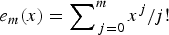 $e_m (x) = \sum\nolimits_{\,j = 0}^m {x^j /j!} $ is the truncated exponential series.
For the denominator in these expressions, as defined in Eq. (5),  $D_k (G,0)$, one can find, by using the approximation of the exponential integral
 $\int_{ne^{ - I^\ast}} ^n {(e^{ - t} /t)} {\kern 1pt} dt\sim(I^\ast - \log n)\exp {\kern 1pt} ( - ne^{ - I^\ast} ),$
 $$\eqalign{D_k (G,0) & \simeq \displaystyle{{n^G ( - 1)^{G - k}} \over {(G - k)!}} \cr & \quad \times \left( [I^\ast - \log n]e^{ - ne^{ - I^\ast}} + e^{ - n} \sum\nolimits_{m = 0}^{G - k - 1} {\displaystyle{{( - 1)^m m!} \over {n^{m + 1}}}} \right. \cr &\quad \left. - e^{ - ne^{ - I^\ast}} \sum\nolimits_{m = 0}^{G - k - 1} {\displaystyle{{( - 1)^m m!} \over {(ne^{ - I^\ast} )^{m + 1}}}} \right) \cr & \quad + e^{GI^\ast} (k - 1)!\left( {1 - e^{ - ne^{ - I^\ast}} \sum\nolimits_{m = 0}^{k - 1} {\displaystyle{{(ne^{ - I^\ast} )^m} \over {m!}}}} \right) \cr & \simeq \displaystyle{{n^G ( - 1)^{G - k}} \over {(G - k)!}} \left( (I^\ast - \log n)e^{ - ne^{ - I^\ast}} \right. \cr &\quad\left.+ e^{ - ne^{ - I^\ast}} \sum\nolimits_{m = 0}^{G - k - 1} {\displaystyle{{( - 1)^{m + 1} m!} \over {(ne^{ - I^\ast} )^{m + 1}}}} \right) \cr & \quad + e^{GI^\ast} (k - 1)!\left( {1 - e^{ - ne^{ - I^\ast}} \sum\nolimits_{m = 0}^{k - 1} {\displaystyle{{(ne^{ - I^\ast} )^m} \over {m!}}}} \right),}$$
or in the still more simplified form
 $$\eqalign{\tilde D_k (G,0) & \simeq \displaystyle{{n^G ( - 1)^{G - k}} \over {(G - k)!}}(I^\ast - \log n)e^{ - ne^{ - I^\ast}} \cr &\quad + e^{GI^\ast} (k - 1)!\left( {1 - e^{ - ne^{ - I^\ast}} \sum\limits_{m = 0}^{k - 1} {\displaystyle{{(ne^{ - I^\ast} )^m} \over {m!}}}} \right),}$$
keeping only the dominating terms. Taking  $ne^{ - I} = x$ and
 $ne^{ - I^\ast} = x^\ast $, the approximate expressions for the pdf in the limits I* ≥ I, equivalently to
 $x^\ast \le x$, and I* < I, equivalently to x* < x, for
 $f^{(G)} (I) \to \tilde f^{(G)} (x)$ read
 $$\eqalign{&\tilde{f}^{(G)} (x) = \cr &\left\{\matrix{e^{ - x} \left(\displaystyle{n \over x} \right)^G \sum\nolimits_{k = 1}^G \displaystyle{x^k \over D_{\rm K} (G,0)} + xe^{ - x} e_{n - G - 1} (x),\quad {\rm for} \;x^{\ast} \le x \comma I^{\ast} \ge I, \hfill \cr e^{ - x} \left(\displaystyle{n \over x^{\ast}} \right)^G \sum\nolimits_{k = 1}^G \displaystyle{x^k \over D_k (G,0)} + xe^{ - x} \left(\displaystyle{x \over x^{\ast}} \right)^G e_{n - G - 1} (x),\quad {\rm for}\; x^{\ast} \gt x \comma I^{\ast} \lt I \comma} \hfill \right.}$$
For the case that the gain G assumes the value of an entire number, the sum in the expression for the pdf simplifies, such that for x* < x we obtain
 $$\eqalign{\tilde f^{(G)} (x) & = e^{ - x} n^G \sum\limits_{k = 1}^{G - 1} {\displaystyle{{x^{k - G}} \over {D_k (G,0)}}} + \displaystyle{{e^{ - x} n^G} \over {D_{k = G} (G,0)}} \cr & \quad+ xe^{ - x} e_{n - G - 1} (x).}$$
The first part of the sum contains, for odd integer G, two neighboring peak terms of the same value, for  $k = [G/2]$ and
 $[G/2] + 1$, and for even integer G, a single peak term for k = G/2. The second part of the sum yields a “plateau”-like term, and the last part is exponentially decreasing.
In terms of x and x* the denominators D k(G, 0) and  $\tilde D_k (G,0)$ are given by
 $$\eqalign{&D_k (G,0) \simeq \displaystyle{{n^G ( - 1)^{G - k}} \over {(G - k)!}} \cr & \times \left( ( - \log x^\ast )e^{ - x^\ast} + e^{ - n} \sum\nolimits_{m = 0}^{G - k - 1} {\displaystyle{{( - 1)^m m!} \over {n^{m + 1}}}} \right. \cr &\left. - e^{ - x^\ast} \sum\nolimits_{m = 0}^{G - k - 1} {\displaystyle{{( - 1)^m m!} \over {(x^\ast )^{m + 1}}}} \right) \cr & + \left( {\displaystyle{n \over {x^\ast}}} \right)^G (k - 1)!\left( {1 - e^{ - x^\ast} \sum\nolimits_{m = 0}^{k - 1} {\displaystyle{{(x^\ast )^m} \over {m!}}}} \right)}$$
and
 $$\eqalign{\tilde D_k (G,0) & \simeq \displaystyle{{n^G ( - 1)^{G - k}} \over {(G - k)!}}( - \log x^\ast )e^{ - x^\ast} \cr & \quad+ \left( {\displaystyle{n \over {x^\ast}}} \right)^G (k - 1)!\left( {1 - e^{ - x^\ast} \sum\limits_{m = 0}^{k - 1} {\displaystyle{{(x^\ast )^m} \over {m!}}}} \right).}$$
We express in the following the pdf from the general expression Eq. (3) for selected values of G.
Approximations of the pdf for selected cases
For G = 1/2 one obtains
 $$f^{(1/2)} (I) \simeq e^{ - ne^{ - I}} e^{(1/2)\min (I,I^\ast )} e^{ - I} \displaystyle{{\sqrt n} \over {\sqrt {\rm \pi}}} \left( {1 + \sum\limits_{k = 1}^{n - 1} {\displaystyle{{(2ne^{ - I} )^k} \over {(2k - 1)!!}}}} \right),$$
and for G = 3/2
 $$\eqalign{\,f^{(3/2)} (I) & \simeq \displaystyle{{e^{ - ne^{ - I}} e^{(3/2)\min (I,I^\ast )} ne^{ - I}} \over {n^{3/2} \int_{ne^{ - I}} ^n {\displaystyle{{e^{ - t}} \over {t^{3/2}}}} dt + (1 - e^{ - ne^{ - I^\ast}} )e^{(3/2)I^\ast}}} \cr & \quad + \displaystyle{{e^{ - ne^{ - I}} e^{(3/2)\min (I,I^\ast )} n^2 e^{ - 2I}} \over {n^{3/2} \sqrt {\rm \pi}}} \cr & \quad \times \left( {1 + \sum\limits_{k = 1}^{n - 2} {\displaystyle{{(2ne^{ - I} )^k} \over {(2k - 1)!!}}}} \right)}$$
For the most interesting case G = 1, we obtain
 $$\eqalign{\,f^{(1)} (I) & \simeq \displaystyle{{e^{ - ne^{ - I}} e^{\min (I,I^\ast )} ne^{ - I}} \over {n\int_{ne^{ - I}} ^n {\displaystyle{{e^{ - t}} \over t}} dt + (1 - e^{ - ne^{ - I^\ast}} )e^{I^{\rm \ast}}}} \cr & \quad+ e^{ - ne^{ - I}} e^{\min (I,I^\ast )} ne^{ - 2I} e_{n - 2} (ne^{ - I} ).}$$
Finally, we give an approximate expression for non-integer G-values:
 $$\eqalign{f^{(G)} (I) &\simeq e^{ - ne^{ - I}} e^{G\min (I,I^{\ast})} \cr & \quad \times \left(\sum\limits_{k = 1}^{[G]} \displaystyle{(ne^{ - I})^k \over n^G \int_{ne^{ - I}}^n \displaystyle{e^{ - t} \over t^{1 + G - k}} dt + e^{GI^{\ast}} \int_0^{ne^{ - I}} \displaystyle{e^{ - t} \over t^{1 - k}} dt} \right. \cr & \left.\qquad + \sum\limits_{k = [G] + 1}^n \displaystyle{(ne^{ - I})^k \over n^G \Gamma (k - G)} \right).}$$