2 Problem formulation and numerical methods

We investigate numerically the dynamics of a dilute polymer solution flowing through a straight circular pipe at a constant flow rate. Polymer dynamics is modelled using the FENE-P model (Bird, Dotson & Johnson Reference Bird, Dotson and Johnson1980). Individual polymer molecules are represented in this model as two inertialess spherical beads connected by a straight nonlinear spring. The orientation and elongation of each polymer molecule is determined by the end-to-end vector $\boldsymbol{q}$ connecting the two beads. The ensemble average of the tensor product of all end-to-end vectors defines a positive–definite symmetric polymer conformation tensor, $\unicode[STIX]{x1D63E}=\langle \boldsymbol{q}\otimes \boldsymbol{q}\rangle$ , which allows the problem to be formulated from a continuum medium approach.

2.1 Governing equations and dimensionless parameters

The governing equations are presented directly in dimensionless form. The pipe radius $R$ , the laminar centreline velocity $u_{lc}$ and the dynamic pressure $\unicode[STIX]{x1D70C}u_{lc}^{2}$ were chosen as characteristic scales for length, velocity and pressure respectively; $\boldsymbol{q}$ was normalized with $\sqrt{kT_{e}/H}$ , where $k$ denotes the Boltzmann constant, $T_{e}$ is the absolute temperature and $H$ is the spring constant. The maximum polymer extension is indicated by the dimensionless parameter $L=q_{0}/\sqrt{kT_{e}/H}$ , where $q_{0}$ is the maximum separation between beads allowed by the spring. Cylindrical coordinates $(z,\unicode[STIX]{x1D703},r)$ are used.

The temporal evolution of $\unicode[STIX]{x1D63E}$ is obtained by solving the following constitutive equation

(2.1) $$\begin{eqnarray}\displaystyle \unicode[STIX]{x2202}_{t}\unicode[STIX]{x1D63E}+\boldsymbol{v}\boldsymbol{\cdot }\unicode[STIX]{x1D735}\unicode[STIX]{x1D63E}=\unicode[STIX]{x1D63E}\boldsymbol{\cdot }\unicode[STIX]{x1D735}\boldsymbol{v}+(\unicode[STIX]{x1D735}\boldsymbol{v})^{\text{T}}\boldsymbol{\cdot }\unicode[STIX]{x1D63E}-\unicode[STIX]{x1D749}, & & \displaystyle\end{eqnarray}$$

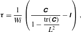
where $\boldsymbol{v}=(u,v,w)$ is the velocity vector field and $\unicode[STIX]{x1D749}$ is the polymer stress tensor. The first two terms on the right-hand side of (2.1) model polymer stretching due to hydrodynamic forces, whereas $\unicode[STIX]{x1D749}$ represents the relaxation forces bringing the polymers back to its equilibrium configuration. $\unicode[STIX]{x1D749}$ is computed using the Peterlin closure

(2.2) $$\begin{eqnarray}\displaystyle \unicode[STIX]{x1D749}={\displaystyle \frac{1}{Wi}}\left({\displaystyle \frac{\unicode[STIX]{x1D63E}}{1-{\displaystyle \frac{\text{tr}(\unicode[STIX]{x1D63E})}{L^{2}}}}}-\unicode[STIX]{x1D644}\right), & & \displaystyle\end{eqnarray}$$

where $\text{tr}(\unicode[STIX]{x1D63E})$ denotes the trace of the polymer conformation tensor, $\unicode[STIX]{x1D644}$ is the unit tensor and $Wi$ is the Weissenberg number; a dimensionless number quantifying the ratio of the polymer relaxation time $\unicode[STIX]{x1D706}$ to the characteristic flow time scale $R/u_{lc}$ .

The fluid motion is governed by the continuity and Navier–Stokes equations

(2.3) $$\begin{eqnarray}\displaystyle & \displaystyle \unicode[STIX]{x1D735}\boldsymbol{\cdot }\boldsymbol{v}=0, & \displaystyle\end{eqnarray}$$

(2.4) $$\begin{eqnarray}\displaystyle & \displaystyle \unicode[STIX]{x2202}_{t}\boldsymbol{v}+\boldsymbol{v}\boldsymbol{\cdot }\unicode[STIX]{x1D735}\boldsymbol{v}=-\unicode[STIX]{x1D735}P+{\displaystyle \frac{\unicode[STIX]{x1D6FD}}{Re}}\unicode[STIX]{x1D6FB}^{2}\boldsymbol{v}+{\displaystyle \frac{(1-\unicode[STIX]{x1D6FD})}{Re}}\unicode[STIX]{x1D735}\boldsymbol{\cdot }\unicode[STIX]{x1D749}+{\displaystyle \frac{4(1+\unicode[STIX]{x1D6FC})}{Re}}\hat{e_{z}}, & \displaystyle\end{eqnarray}$$

where $P$ is the pressure, $\unicode[STIX]{x1D6FD}=\unicode[STIX]{x1D708}_{s}/\unicode[STIX]{x1D708}$ measures the relative importance between the solvent viscosity $\unicode[STIX]{x1D708}_{s}$ and the viscosity of the solution at zero shear rate $\unicode[STIX]{x1D708}$ , $Re=u_{lc}R/\unicode[STIX]{x1D708}$ is the Reynolds number and $\unicode[STIX]{x1D6FC}$ is the fluctuating pressure gradient required to keep a constant mass flux. Polymers modify the dynamics of Newtonian flows through polymer stresses. These are incorporated into the conventional Navier–Stokes equation through the divergence of the polymer stress tensor. The $(1-\unicode[STIX]{x1D6FD})$ prefactor multiplying this term indicates the contribution of the polymers to the total viscosity and must be small for a dilute polymer solution. Periodic boundary conditions are used in the streamwise $z$ and azimuthal $\unicode[STIX]{x1D703}$ directions, whereas the no-slip condition is imposed at the pipe wall $r=R$ .

In all simulations presented in this paper the Reynolds number was fixed to $Re=3500$ , for which the flow is turbulent in the Newtonian case, and $Wi$ was used as control parameter. We also fixed $\unicode[STIX]{x1D6FD}$ to $0.9$ which is the value corresponding to the experiments of C,L&H at a concentration of $90$ ppm. Given the values of $\unicode[STIX]{x1D6FD}$ and $L$ , polymers can be characterized by their extensibility number $E_{x}=2L^{2}(1-\unicode[STIX]{x1D6FD})/3\unicode[STIX]{x1D6FD}$ (Xi & Graham Reference Xi and Graham2010b ). For our simulations we have considered two different polymers with very different extensibilities. The maximum extension of the first polymer type, $L=30$ , was chosen so that its extensibility number, $E_{x}=66.6$ , coincides with one of the cases presented in Xi & Graham (Reference Xi and Graham2010b ). The second polymer type has a very high extensibility, $E_{x}=2962.96$ for $L=200$ , and it corresponds to the parameters used in simulations of elasto-inertial turbulence by Dubief et al. (Reference Dubief, Terrapon and Soria2013). These two cases will be henceforth referred to as moderate extensibility ME and large extensibility LE cases, respectively.

2.2 Numerical methods

The governing equations are solved in primitive variables using a highly scalable pseudo-spectral solver recently developed in house. The code is parallelized using a combination of the MPI and OpenMP programming models (see Shi et al. (Reference Shi, Rampp, Hof and Avila2015) for further details). Spatial discretization in the two periodic directions, $z$ and $\unicode[STIX]{x1D703}$ , is accomplished via Fourier–Galerkin expansions, whereas central finite differences on a Gauss–Lobatto–Chebyshev grid are used in $r$ . Pressure and velocity in (2.4) are decoupled through a pressure Poisson equation (PPE) formulation. An influence matrix is used to impose the free divergence boundary condition directly on velocity, thereby avoiding the use of artificial pressure boundary conditions. The equations for the azimuthal and radial velocity components $v$ and $w$ are decoupled using the change of variables, $u_{+}=w+\text{i}v$ and $u_{-}=w-\text{i}v$ (Orszag & Patera Reference Orszag and Patera1983).

The time integration was carried out using a second order accurate predictor–corrector scheme based on the Crank–Nicolson method (Willis Reference Willis2017). For a generic variable $\boldsymbol{X}$ at a time $n$ the predictor equation reads

(2.5) $$\begin{eqnarray}\displaystyle \left({\displaystyle \frac{1}{\unicode[STIX]{x1D6FF}t}}-\text{i}c\unicode[STIX]{x1D6FB}^{2}\right)\boldsymbol{X}_{1}^{n+1}=\left({\displaystyle \frac{1}{\unicode[STIX]{x1D6FF}t}}+(1-\text{i}c)\unicode[STIX]{x1D6FB}^{2}\right)\boldsymbol{X}^{n}+\boldsymbol{N}^{n}, & & \displaystyle\end{eqnarray}$$

where $\boldsymbol{N}$ denotes the nonlinear terms, $\unicode[STIX]{x1D6FF}t$ is the time step size and the constant $\text{i}c$ defines the implicitness of the method ( $\text{i}c=0.5$ in our simulations). The initial estimate $\boldsymbol{X}_{1}^{n+1}$ is then refined following an iterative correction procedure. At each corrector iteration the nonlinear terms are re-evaluated and $\boldsymbol{X}_{j}^{n+1}$ is obtained solving the following equation

(2.6) $$\begin{eqnarray}\displaystyle \left({\displaystyle \frac{1}{\unicode[STIX]{x1D6FF}t}}-\text{i}c\unicode[STIX]{x1D6FB}^{2}\right)\boldsymbol{X}_{k+1}^{n+1}=\left({\displaystyle \frac{1}{\unicode[STIX]{x1D6FF}t}}+(1-\text{i}c)\unicode[STIX]{x1D6FB}^{2}\right)\boldsymbol{X}^{n}+\text{i}c\boldsymbol{N}_{k}^{n+1}+(1-\text{i}c)\boldsymbol{N}^{n}, & & \displaystyle\end{eqnarray}$$

where $k=1,2,\ldots \,$ . The iteration loop stops when $\Vert \boldsymbol{X}_{k+1}^{n+1}-\boldsymbol{X}_{k}^{n+1}\Vert \leqslant 10^{-6}$ . Convergence usually occurs after one iteration of the corrector step. The additional computational cost of computing the advective terms twice at each time step is compensated by the larger $\unicode[STIX]{x1D6FF}t$ allowed by this temporal scheme in comparison with other conventional methods. The source terms in (2.1) and the term containing the divergence of the polymer stress tensor in (2.4) are treated as nonlinear terms. Note that (2.1) is hyperbolic and does not have any diffusive term ( $\unicode[STIX]{x1D6FB}^{2}\boldsymbol{X}$ ). This lack of dissipation leads to numerical error accumulation which often causes spurious instabilities and numerical breakdown. To avoid these problems we incorporate a small amount of artificial diffusion to our simulations which enhances numerical stability. This is accomplished by adding a Laplacian term $(1/ReS_{c})\unicode[STIX]{x1D6FB}^{2}\unicode[STIX]{x1D63E}$ to the right-hand side of (2.1), where $S_{c}=\unicode[STIX]{x1D708}/\unicode[STIX]{x1D705}$ is the Schmidt number quantifying the ratio between the viscous and artificial diffusivities. Unless otherwise specified, the simulations presented in this paper were performed using $S_{c}=0.5$ . This yields an artificial diffusion coefficient $(1/ReS_{c})\sim O(10^{-4})$ which is of the same order of magnitude as in Xi & Graham (Reference Xi and Graham2010b ), and quite below those of early works, e.g. Ptasinsky et al. (Reference Ptasinsky, Boersma, Nieuwstadt, Hulsen, Van den Brule and Hunt2003), Sureshkumar, Beris & Handler (Reference Sureshkumar, Beris and Handler1997), where $(1/ReS_{c})\sim O(10^{-2})$ . With the inclusion of this Laplacian term two boundary conditions are needed: as suggested in Beris & Dimitropoulos (Reference Beris and Dimitropoulos1999) we impose that $\unicode[STIX]{x1D63E}$ at $r=R$ must be the same as without artificial diffusion, whereas symmetry boundary conditions are used at $r=0$ .

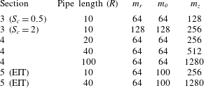
The numerical resolution of the simulations presented in this paper is shown in table 1; $\unicode[STIX]{x1D6FF}t$ is dynamically adjusted to ensure that the Courant–Friedrichs–Lewy (CFL) condition always remains below $0.25$ .

Table 1.

Number of radial nodes, $m_{r}$ , and Fourier modes, $m_{\unicode[STIX]{x1D703}}$ and $m_{z}$ , used in the simulations.

3 Dynamics of viscoelastic pipe flow turbulence in short computational domains

Figure 1.

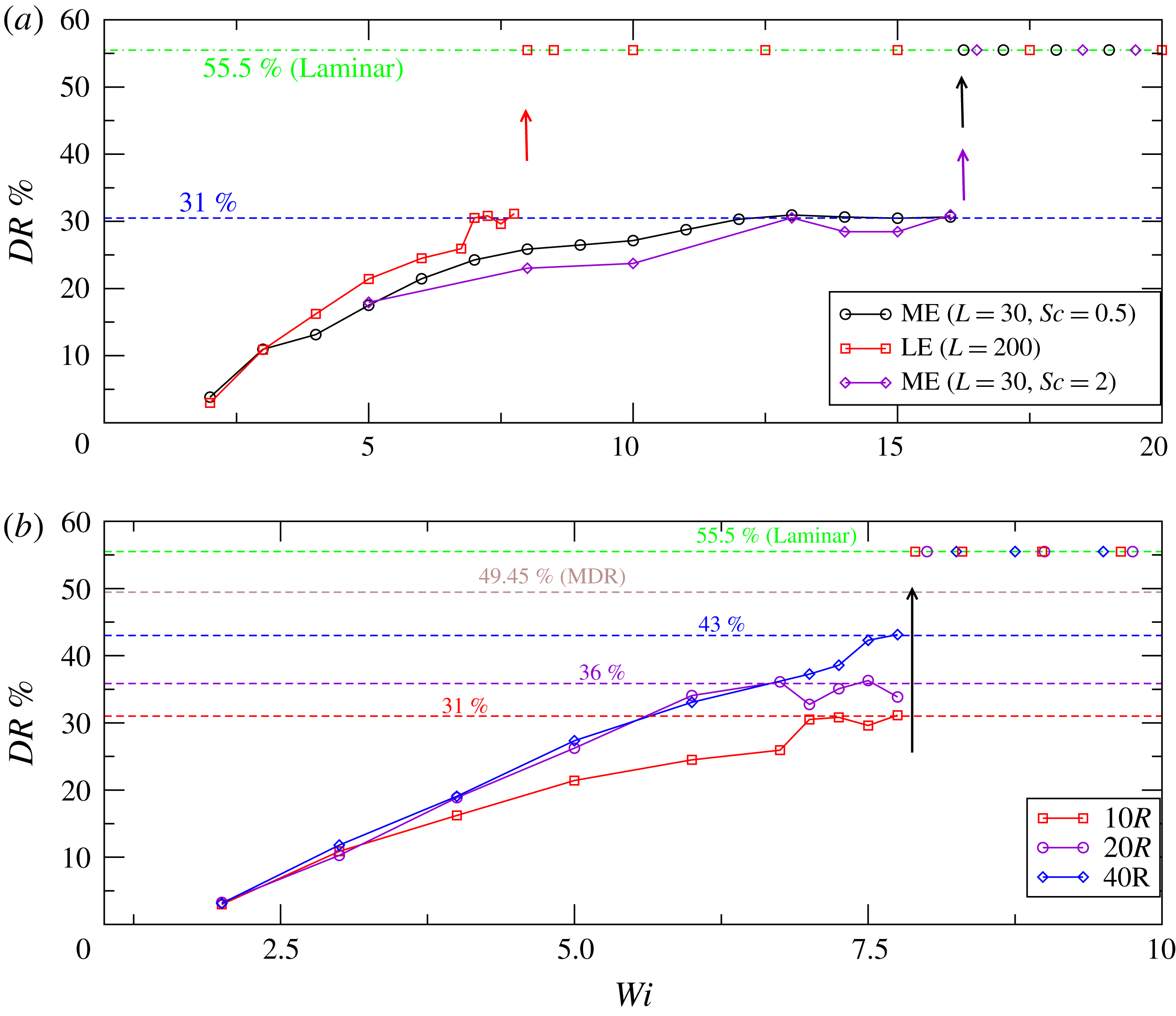
Evolution of the drag reduction percentage $DR\,\%$ with increasing $Wi$ up to where relaminarization occurs in pipe flow simulations performed at $Re=3500$ . (a) Simulations carried out in a $10R$ long pipe using two polymers with different extensibilities: LE (large extensibility, $L=200$ ) and ME (moderate extensibility, $L=30$ ). Diamonds (purple line) illustrate the effect of reducing the global artificial diffusion. (b) Variation of $DR\,\%$ as the pipe length is varied for the LE case. The green and brown dashed lines show the drag reduction level of the laminar and MDR states, respectively, whereas the remaining dashed lines indicate the maximum drag reduction achieved in each case. Arrows indicate the $Wi$ at which flow relaminarization occurs.

Because of the additional equations for $\unicode[STIX]{x1D63E}$ and $\unicode[STIX]{x1D749}$ , viscoelastic turbulence simulations are in computational terms far more demanding than Newtonian simulations. A common approach to minimize the computational cost is to choose the smallest domain size that computes reasonably accurate dynamics. On that basis, we have set the pipe length to $L_{z}=10R$ , which is nearly the minimum size needed in Newtonian pipe flow simulations to ensure that these are unaffected by streamwise periodicity. The simulations were performed according to the following procedure. Starting from a fully turbulent Newtonian solution, we increased $Wi$ progressively by one unit, with the exception of the range $6\leqslant Wi\leqslant 8$ in the LE case, where $Wi$ was varied in intervals of $0.25$ . The simulations were run over $2000R/u_{lc}$ time units and as initial condition we used a previously computed solution with $Wi$ close to that being computed. The averaged drag reduction percentage was calculated as $DR\%=(f_{N}-f)/f_{N}$ , where $f_{N}$ and $f$ are the average friction factors for the Newtonian and viscoelastic cases respectively. The former is given by the Blasius friction law, $f_{N}=0.079Re^{-0.25}$ , whereas the latter is calculated from the Fanning friction formula, $f=\unicode[STIX]{x1D70F}_{w}/2\unicode[STIX]{x1D70C}U_{b}^{2}$ , where $U_{b}$ , $\unicode[STIX]{x1D70F}_{w}$ and $\unicode[STIX]{x1D70C}$ are the bulk velocity, average wall shear stress and fluid density respectively. For each $Wi$ , a set of $10$ simulations was performed and the drag reduction level was computed by averaging over the ensemble of the simulations.

As shown in figure 1(a), even for two simulations mimicking different polymers, the same qualitative scenario in terms of drag reduction is obtained. The amount of drag reduction increases continuously with increasing $Wi$ up to a critical threshold after which the flow relaminarizes. A clear effect of increasing the maximum polymer extension $L$ is that the dynamics is accelerated: the polymer with higher extensibility LE produces for the same $Wi$ significantly larger drag reduction than the ME polymer, and it eventually causes relaminarization at a much lower value of $Wi$ , $Wi_{lam}=7.75$ , than in the ME case, $Wi_{lam}=16$ . We note here that, as $Wi_{lam}$ is approached, the simulations become sensitive to the initial condition and turbulence does not always survive over the time threshold chosen. The critical values for relaminarization $Wi_{lam}$ given above correspond to the highest values of $Wi$ for which turbulence survives in more than $50\,\%$ of the simulations performed. There are also certain ranges of $Wi$ at which polymer extensibility does not appear to play any role. For example, at very low $Wi$ ( $W\leqslant 3$ ), the degree of polymer stretching is low and both polymers, despite having very different extensibility, produce nearly the same drag reduction. A much more surprising effect occurs at larger $Wi$ prior to relaminarization. Here, the drag reduction approaches an almost constant level, $31\,\%$ , regardless of the polymer extensibility. This levelling off was observed in the earlier study of Xi & Graham (Reference Xi and Graham2010b ) and suggested as an asymptotic regime (AR). In the present study, the AR occurs over a narrow range of $Wi$ , and since dynamical changes take place faster for higher extensibility, it is much more evident in the ME case, $12\leqslant Wi\leqslant 16$ , than in the LE case, $6.75\leqslant Wi\leqslant 7.75$ .

Figure 2.

Temporal intermittency. (a) Shows the temporal evolution of the friction factor $f$ for the ME case and $Wi=13$ , whereas (b,c) illustrate instantaneous mean velocity profiles at low and high friction events. Note that here velocity ( $U^{+}$ ) and radius ( $r^{+}$ ) are expressed in inner units, i.e. normalized with the friction velocity ( $u_{\unicode[STIX]{x1D70F}}=\sqrt{\unicode[STIX]{x1D70F}_{w}/\unicode[STIX]{x1D70C}}$ ) and the viscous length ( $\unicode[STIX]{x1D6FF}_{\unicode[STIX]{x1D708}}=\unicode[STIX]{x1D708}/u_{\unicode[STIX]{x1D70F}}$ ) respectively.

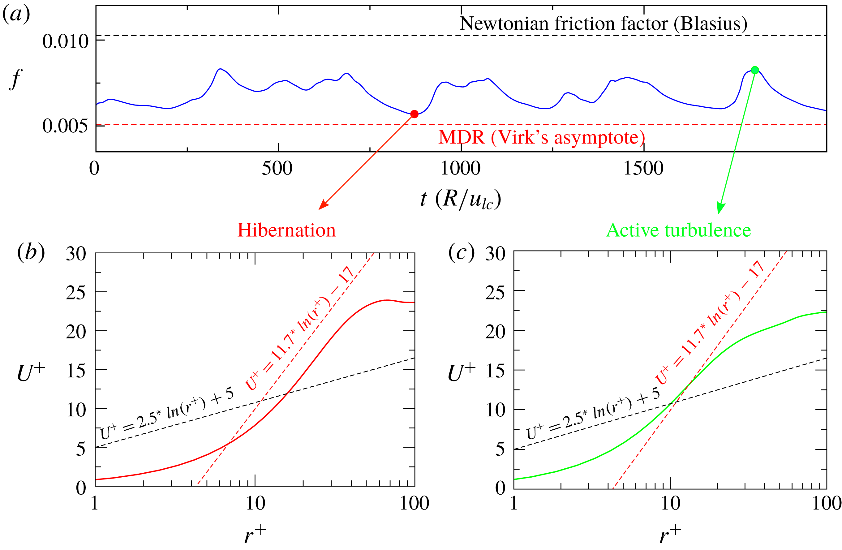
A key feature of the dynamics in these simulations is the presence of temporal intermittency, with periods of low friction which are interspersed with other periods of higher friction, as shown in figure 2. This intermittent dynamics is also in agreement with the simulations of Xi & Graham (Reference Xi and Graham2010b , Reference Xi and Graham2012b ), who dubbed the low and high friction intervals as hibernating and active turbulence, respectively. The frequency and duration of hibernating events increases progressively with increasing $Wi$ , and the friction associated with active turbulent events decreases as $Wi$ increases, leading to the gradual growth in average drag reduction shown in the figure 1(a). To further illustrate the distinction between hibernating and active turbulence, the bottom panel in figure 2 shows instantaneous velocity profiles in inner units corresponding to each state. The black and red dashed lines in these figures show the logarithmic laws that have been traditionally used to describe the mean velocity profile in the logarithmic layer ( $30\lessapprox r^{+}\lessapprox 60$ , for $Re=3500$ ) for wall bounded Newtonian turbulence (Prandtl–Kármán law) and viscoelastic turbulence at MDR (Virk’s asymptote), respectively. It should be noted that the functional form of the mean velocity profile at MDR is not truly logarithmic (White et al. Reference White, Dubief and Klewicki2012; Elbing et al. Reference Elbing, Perlin, Dowling and Ceccio2013) and so the Virk’s asymptote should be understood as an idealization of velocity profiles in this limit. Hibernating events are characterized by velocity profiles that notably deviate from the Prandtl–Kármán law and become nearly parallel to Virk’s asymptote profile throughout the logarithmic layer. By contrast, in active turbulence events, although friction may be substantially lower than that for pure Newtonian turbulence, the profile in the log layer has a comparable slope to the Prandtl–Kármán law. On the basis of similar observations, it has been argued that states of active turbulence have similar properties to Newtonian turbulence, whereas hibernating events could be directly connected to MDR. More specifically, it was suggested that MDR might be a state fully dominated by hibernation, which is achieved asymptotically as $Wi$ is increased (Xi & Graham Reference Xi and Graham2010a ). However, in our simulations, as well as in previous simulations reporting this intermittent scenario, the flow eventually relaminarizes with increasing $Wi$ and an asymptotic state (the AR) is reached only over a narrow range of $Wi$ prior to relaminarization. Since the AR exhibits some features of MDR: saturation of the drag reduction level with increasing $Wi$ and comparable results are obtained for different polymer properties, it has been interpreted as the first numerical evidence of MDR. However, there is also evidence which appears to indicate that the AR does not correspond to MDR. Firstly, while hibernation is prominent in this regime, active turbulence events also occur frequently, and so the average drag reduction level at AR ( $31\,\%$ ) is considerably less than that of MDR at $Re=3500$ ( $49.5\,\%$ ). Another distinctive feature is that in the AR the saturation of drag reduction occurs over a finite range of $Wi$ and upon further increase in $Wi$ the flow relaminarizes. In contrast, MDR is a persistent state and the drag reduction level remains nearly unchanged as $Wi$ increases. Finally, it should also be noted that temporal intermittent dynamics such as that previously described has not been reported in experiments at MDR. It is therefore unclear whether the dynamics of the AR may be related to MDR.

Before proceeding further, we want to briefly discuss the impact that the artificial diffusion added to (2.1) has on the reported scenario. Sid, Terrapon & Dubief (Reference Sid, Terrapon and Dubief2018) recently showed that adding polymer diffusion substantially weakens the elastic scales at large $Wi$ . They found that this effect is particularly relevant in the elasto-inertial turbulent regime, where elastic scales play a crucial role in feeding turbulence and thus an excessive polymer diffusion leads to flow relaminarization. As will be shown later, the simulations described in this section do not correspond to the elasto-inertial regime. However, it is important to clarify whether the relaminarization observed might also be an artefact of the artificial polymer diffusion. If the relaminarization were caused by the diffusive term, one would expect that as $S_{c}$ is increased, i.e. as the amount of diffusion is reduced, the relaminarization threshold would progressively shift towards larger values of $Wi$ , until eventually, at a sufficiently large $S_{c}$ , the relaminarization does not take place any more. To examine how the polymer diffusion affects the relaminarization threshold, simulations for the case of moderate extensibility, decreasing the amount of diffusion by a factor of $4$ ( $S_{c}=2$ ), were performed following the same procedure described above. As seen in figure 1(a) (diamonds), the flow relaminarization in these simulations was found to occur at the same value of $Wi$ ( $Wi_{lam}=16$ ) as in the simulations using $S_{c}=0.5$ . This insensitivity of the relaminarization threshold to changes in $S_{c}$ suggests that the relaminarization phenomenon is not driven by polymer diffusion but rather a robust feature of these simulations. We also note that, while quantitative differences exist between simulations with $S_{c}=0.5$ and $2$ , i.e. less polymer diffusion produce less drag reduction, the same qualitative scenario is observed in both cases: the amount of drag reduction increases with increasing $Wi$ up to a regime is reached (the AR) where it remains nearly constant. Based on these observations, we argue that polymer diffusion only has a moderate influence at these $Wi$ and does not affect significantly the results discussed in this paper.

4 Simulations in larger computational domains: reverse transition

To assess the influence of the pipe length in the results of § 3, the same computational procedure was repeated using larger pipes ( $20R$ and $40R$ ). A comparison of the drag reduction scenario obtained for the LE polymer when the pipe length was varied is shown in figure 1(b). A first interesting observation is that, consistent with other works on viscoelastic turbulence (Li, Sureshkumar & Khomami Reference Li, Sureshkumar and Khomami2006; Wang, Shekar & Graham Reference Wang, Shekar and Graham2017), viscoelasticity increases the streamwise correlation length with respect to Newtonian simulations. Hence, while at these low $Re$ a streamwise length of $10R$ is enough to obtain realistic statistics in Newtonian pipe flow, viscoelastic simulations are still affected by streamwise periodicity and result in lower drag reduction than those obtained when larger pipes are used. Simulations performed in $20R$ and $40R$ long pipes produce nearly the same drag reduction up to $Wi\sim 6.75$ , but differ both quantitatively and qualitatively when relaminarization is approached. For simulations using a $20R$ long pipe, the same qualitative scenario as in the $10R$ long pipe simulations is found: the drag reduction remains nearly constant over a finite range of $Wi$ , $6\leqslant Wi\leqslant 8$ , before relaminarization takes place. However, when a pipe of $40R$ is used, this AR disappears and the drag reduction increases monotonically with increasing $Wi$ until the flow relaminarizes. This observation suggests that rather than being a manifestation of MDR, the AR might be a consequence of the streamwise periodicity imposed in the simulations and thus it might lack practical significance.

An additional test to confirm that the dynamics at the AR is different from that at MDR is to compare the flow structures in our simulations with recent experimental visualizations of MDR structures in pipe flow at low Reynolds numbers (Choueiri et al. Reference Choueiri, Lopez and Hof2018). These experiments showed that turbulence at MDR substantially differs from Newtonian type turbulence and it is characterized by very elongated streaks which are slightly inclined away from the wall (see figure 3 in Choueiri et al. (Reference Choueiri, Lopez and Hof2018)). If the dynamics at the AR corresponded to MDR, similar flow structures should be observed in our simulations, provided that the computational domain is long enough to accommodate them. To examine this possibility, we have performed a new set of simulations using a pipe of $100R$ in the axial direction, which is approximately twice the size of the shortest structures observed by Choueiri et al. (Reference Choueiri, Lopez and Hof2018). Figure 3 illustrates the dynamical evolution of the turbulence structures as $Wi$ was increased in these simulations. It shows, at a certain time instant, the variation of the centreline velocity $u_{c}$ along the pipe (a) and isocontours of the radial velocity $w$ (e) for several $Wi$ representative of different dynamical regimes in the ME case. Note that a Newtonian case (figure 3 a) has also been included for comparison. At low drag reduction ( $Wi<6$ ), the dynamics is very similar to that of the Newtonian case (see panels (a) and (b) in the figure). Turbulence always fills the pipe entirely and the centreline velocity exhibits comparable fluctuation levels in both cases. Nevertheless, the flow structures in the viscoelastic case are broader and slightly more elongated in the axial direction than those in pure Newtonian turbulence, reflecting the drag reduced nature of the flow in viscoelastic simulations. Another clear distinction is that, while turbulence extends across the entire pipe diameter in the Newtonian case, there are several areas in the drag reduced flow where the near wall turbulence has been suppressed by polymer activity. As $Wi$ increases (between $Wi=7$ and $11$ ), the dynamics exhibits a complex spatio-temporal behaviour. As shown in figure 3(c) for $Wi=8$ , turbulence is confined to streamwise localized patches known in the Newtonian pipe flow literature as slugs. The distance between the turbulent fronts, i.e. the interfaces separating laminar from turbulent flow, increases progressively with time until the turbulence eventually fills the entire pipe. This space-filling turbulent state does not persist long and turbulence takes back the form of slugs, thereby restarting the cycle again. With further increase in $Wi$ , coinciding with those $Wi$ at which the AR occurs in shorter pipes, $12\leqslant Wi\leqslant 16$ , turbulence becomes permanently localized in the streamwise direction taking the form of turbulent puffs. As seen in figure 3(e), these viscoelastic puffs are very similar to Newtonian puffs: arrow-headed structures where turbulence is mainly concentrated in the sharp upstream edge and progressively diffuses away as the puff is followed downstream. Unlike slugs, puffs keep their size constant and travel downstream at a nearly constant speed. We also found that these puffs sporadically split into two smaller puff-like structures (see figure 3 d). However, since the domain is not large enough to contain two full-size puffs, there is a strong interaction between them which causes the downstream puff to quickly relaminarize (Hof et al. Reference Hof, de Lozar, Avila, Tu and Schneider2010). We note here that, although the pipe length in these simulations is enough to identify spatially localized structures, these are still affected by the finite size of the computational domain. As a result, laminar flow is not fully recover, i.e. the centreline velocity does not recover its laminar value $u_{c}=1$ , and the length of the simulated puffs is slightly shorter than that in laboratory experiments. Finally, when $Wi$ is increased above $16$ the flow fully relaminarizes, showing that this is a robust feature of these simulations which occurs at the same $Wi$ regardless of the pipe length considered.

Figure 3.

Evolution of the spatio-temporal dynamics and turbulence structures as $Wi$ increases when the simulations are carried out in a long pipe of $100R$ in the streamwise direction. (a) Shows the streamwise variation of the centreline velocity, $u_{c}$ , whereas (e) illustrates isosurfaces of the radial velocity. The flow direction is from left to right. Note that the aspect ratio of the pipe has been increased to facilitate visualization of the structures.

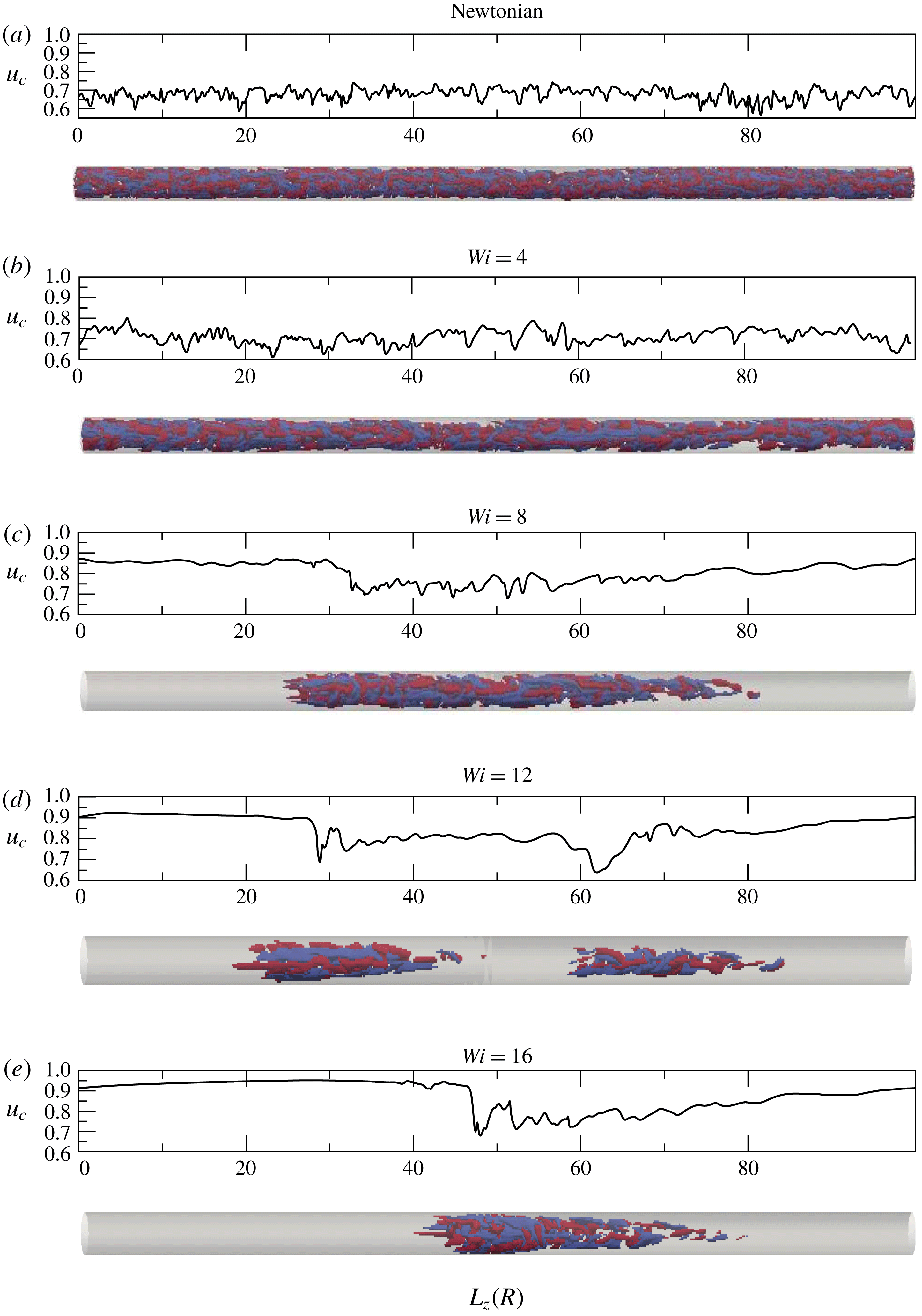
The dynamical scenario described above raises two important points. Firstly, increasing $Wi$ in these simulations leads to a relaminarization scenario which follows the same sequence of states as the transition to turbulence in the Newtonian case but in reverse direction, i.e. turbulence, slugs, puff splitting, puffs and laminar flow. We will henceforth refer to the dynamics of this relaminarization scenario as reverse transitional dynamics. Secondly, the dynamics at the $Wi$ corresponding to the AR, $12\leqslant Wi\leqslant 16$ , is characterized by puffs and this is qualitatively very different from the structures observed at MDR in experiments. It should, however, be noted that the reported scenario only occurs at $Re$ near the turbulence transition and so the conclusions reached from these results strictly apply only in this regime.

Finally, we note that a comparison between temporal dynamics in small (minimal) domains and spatio-temporal dynamics in larger domains at similar Reynolds numbers was also presented in Wang et al. (Reference Wang, Shekar and Graham2017). This study established the similarity between statistics obtained from time series analysis in minimal domains and those obtained by thresholding and conditional average in larger domains. Nevertheless, the axial length for the large domain simulations in this study was fixed to $L_{z}\sim 40h$ ( $h$ is the channel half-width, equivalent to $R$ in our simulations) and thus the effect of further increasing $L_{z}$ was not assessed. When using similar computational domains ( $L_{z}=40R$ ), our simulations reveal that the flow is significantly affected by finite-size effects. The pipe length here is smaller than the axial extent of the turbulent patches shown in figure 3. Hence, using periodic boundary conditions create artificial interactions between the upstream and downstream edges of these turbulent structures. This results in flow states characterized by space-filling turbulence whose intensity varies in space and time, which are similar to those analysed in Wang et al. (Reference Wang, Shekar and Graham2017). An example of these states is shown in figure 4, corresponding to a simulation for $Wi=16$ using a $40R$ long pipe. In contrast to the simulation in a $100R$ long pipe (figure 3 e), where a clear puff is observed, here the flow does not exhibit laminar regions and significant velocity fluctuations coexist with regions of weaker fluctuations along the entire pipe. We argue that, as occur in our simulations, if the simulations presented in Wang et al. (Reference Wang, Shekar and Graham2017) were extended to larger axial domains, the spatio-temporal alternation between hibernating and active turbulent regions described in this paper might turn into the coexistence of fully laminar and turbulent flow regions.

Figure 4.

Same as in figure 3(e) when a pipe of $40R$ in the streamwise direction is used.

5 Comparison with experimental results

The question now is whether the reverse transitional dynamics captured by our simulations provides a meaningful description of viscoelastic pipe flow dynamics, i.e. whether or not these simulations reproduce experimental observations. To answer this question we provide in this section a detailed description of the dynamical scenario found by Choueiri et al. (Reference Choueiri, Lopez and Hof2018) in pipe flow laboratory experiments at a similar Reynolds number, $Re=3150$ , when the polymer concentration $c$ is increased progressively from Newtonian turbulence to MDR (for details about the experimental set-up, see supplementary material in Choueiri et al. (Reference Choueiri, Lopez and Hof2018)). Note that the control parameter in these experiments is polymer concentration, whereas in simulations it is the polymer relaxation time $\unicode[STIX]{x1D706}$ , i.e. $Wi$ , that varies. These two magnitudes are however directly correlated. It has been shown that even in dilute polymer solutions the relaxation time grows with increasing polymer concentration (Giudice, Haward & Shen Reference Giudice, Haward and Shen2017). Hence, increasing $Wi$ in our simulations is related to increasing polymer concentration in experiments. Figure 5(a) shows the variation of the drag reduction percentage as polymer concentration was varied in the experiments. Similarly to what occurs in the simulations, the amount of drag reduction $DR\%$ increases initially with increasing polymer concentration until a threshold value is reached, $c\sim 23$  ppm (parts per million by weight), at which the flow fully relaminarizes. The flow remains laminar regardless of the imposed perturbations over a significant range of polymer concentration ( $c\sim 23{-}43$  ppm). However, for $c>43$  ppm, the flow becomes chaotic again and the drag reduction level approaches progressively that of Virk’s asymptote.

Figure 5.

(a) Evolution of the drag reduction percentage $DR\%$ with increasing polymer concentration (expressed in parts per million by weight ppm) in the experiments of C,L&H for $Re=3150$ . (b–f) LDV measurements of the centreline velocity $u_{c}$ illustrating the changes in the dynamics as polymer concentration increases.

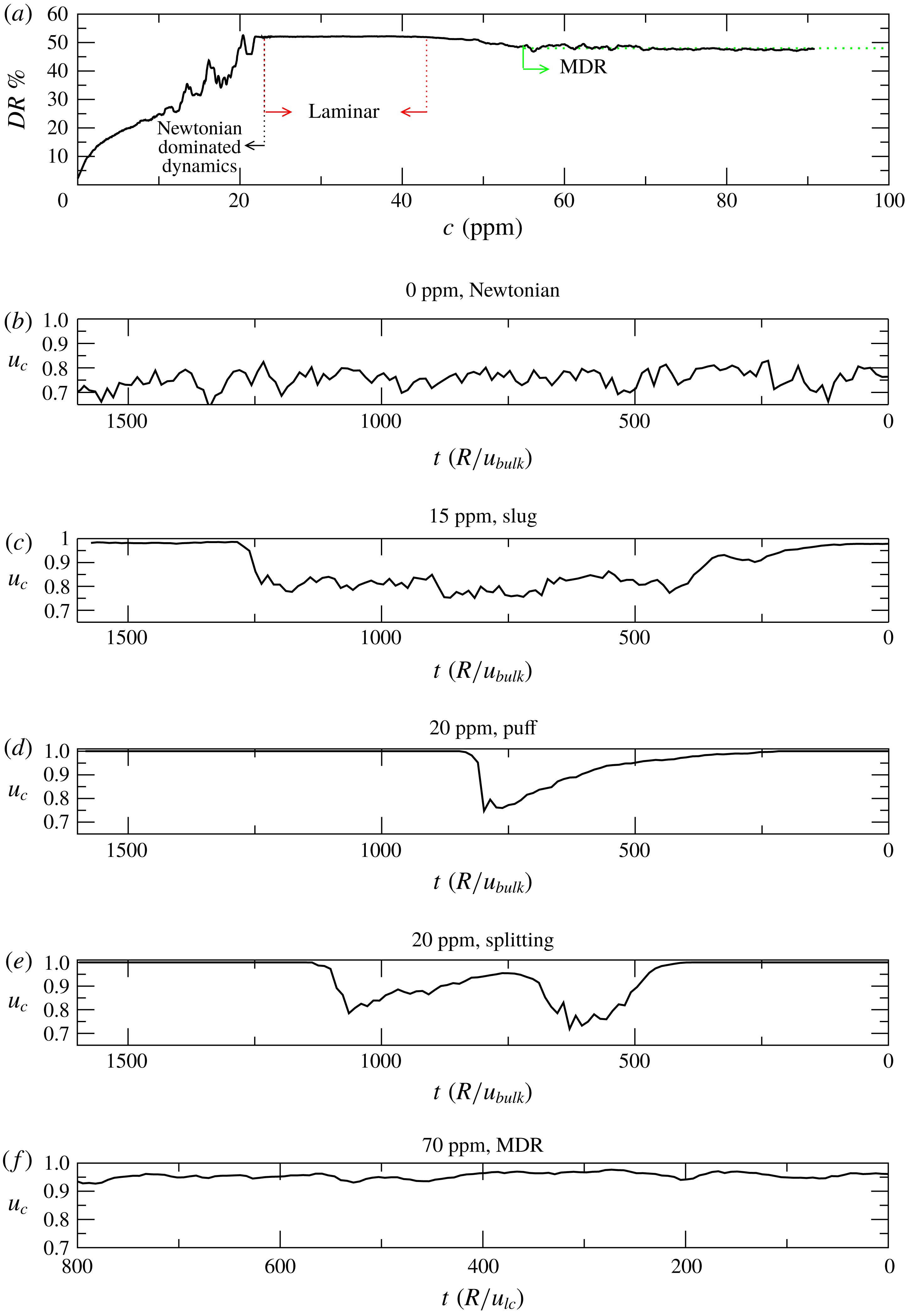
Figure 5(b–f) illustrates how the dynamics changes as the polymer concentration increases. More specifically, these figures show the temporal variation of the centreline velocity $u_{c}$ obtained from laser Doppler velocimetry (LDV) measurements at a central streamwise location. The $x$ -axis has been inverted to facilitate comparison with the instantaneous streamwise distribution of $u_{c}$ shown in figure 3. Note that, as in the simulations, $u_{c}$ is normalized with the centreline velocity of the laminar state. In the absence of polymers (see figure 5 b) the flow is fully turbulent and $u_{c}$ exhibits persistent random amplitude fluctuations. As the polymer concentration is increased ( $c\geqslant 13$  ppm), time intervals where $u_{c}$ strongly fluctuates alternate with others at which it nearly recovers its laminar value (see figure 5 c and compare to the analogous case in the simulations, figure 3 c). This temporal intermittency between turbulent and laminar states indicates that the dynamics at this regime is characterized by spatially localized structures. Furthermore, since the duration of these turbulent and laminar intervals is highly variable, and both trailing and leading edge interfaces show a sharp adjustment of the centreline velocity, it is evident that these localized structures correspond to slugs (Wygnanski & Champagne Reference Wygnanski and Champagne1973). With further increase in concentration ( $c\geqslant 18$  ppm), slugs are replaced by puffs (see figure 5 d and analogous case in the simulations, figure 3 e). These structures are clearly distinguishable because of their long diffusive tail and sharp velocity variation associated with the upstream edge. As occurs in the simulations (figure 3 d), splitting events are also frequently encountered in the experiments (see figure 5 e), leading either to the emergence of slugs or trains of puffs depending on the polymer concentration. When $23$  ppm ${<}c<43$  ppm, turbulence is fully suppressed by the polymers and $u_{c}$ remains constant and equal to the laminar value. It should be emphasized at this point that the dynamics taking place in the experiments is in excellent qualitative agreement with the reverse transition found in the simulations. Ultimately, for $c\geqslant 43$  ppm (see figure 5 f), the flow reaches MDR and $u_{c}$ exhibits again persistent oscillations. The frequency and amplitude of these oscillations are however much lower than those for a fully turbulent Newtonian flow, and the deviation of $u_{c}$ from laminar flow always remains less than 10 %.

The existence of a wide range of polymer concentrations at which the flow is laminar makes a clear distinction between two regimes where polymers play different dynamical roles. In the first regime the role of the polymers is to suppress turbulence and cause a reverse transition. As discussed in § 4, the dynamics in this regime is dominated by the same flow structures as in the Newtonian case and polymers simply act to delay the transition scenario. In the second regime, for $c>43$  ppm, the interplay between high polymer elasticity and inertial effects drives an instability, dubbed in Samanta et al. (Reference Samanta, Dubief, Holzner, Schäfer, Morozov, Wagner and Hof2013) the elasto-inertial instability (EII), which results in a new turbulence type, elasto-inertial turbulence (EIT). As shown in figure 5(a), the drag reduction level associated with EIT is close to that of Virk’s asymptote and it remains unchanged as polymer concentration increases. These observations suggest that at these low Reynolds numbers EIT may be directly related to MDR.

An additional remark about EIT (and thus MDR) is that as seen in figure 5(f), it is always space filling and no spatio-temporal intermittency is observed in this regime. This is an important feature that can help distinguish realistic MDR dynamics from other regimes with similar statistical properties. An example of the latter are the puffs found prior to relaminarization. We found in both simulations and experiments that the average friction coefficient and mean velocity profiles associated with these puffs are nearly identical to those at MDR (not shown). Hence, the circumstance that time averaged statistical quantities match those of MDR (main criterion to identify MDR in many earlier studies) is a necessary but not sufficient condition to identify this regime in numerical simulations. An analysis of the spatio-temporal dynamics must also be carried out to discern whether or not the simulated flows belong to the MDR regime.

6 Elasto-inertial turbulence

Figure 6.

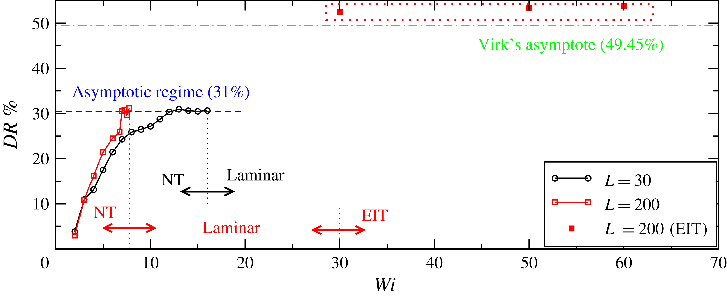
Global scenario, in terms of drag reduction, obtained in simulations using a $10R$ long pipe and polymers with moderate ( $L=30$ ) and large extensibility ( $L=200$ ). The arrows delimit regions with distinct dynamical features. The acronyms NT and EIT denote the Newtonian dominated regime and the elasto-inertial turbulent regime, respectively. The data corresponding to the simulations of EIT presented in § 6 are encircled by a (red) dotted rectangle. Note that the EIT regime was only found in the case of large polymer extensibility.

We have shown so far that our FENEP-NS (Navier–Stokes) simulations qualitatively reproduce the dynamics observed in experiments up to the point where relaminarization occurs. The next question is therefore whether by increasing $Wi$ beyond the relaminarization threshold these simulations are also capable of capturing the EII and MDR. To address this question we have performed several simulations at $Wi$ ranging from $20$ to $80$ in both the ME and LE cases. The pipe length was initially set again to $10R$ . The simulations were initialized from the base flow, previously computed, which was perturbed by adding a pair of streamwise localized rolls ( $v=A(g+rg^{\prime })\cos (\unicode[STIX]{x1D703})\text{e}^{-10\sin ^{2}(\unicode[STIX]{x03C0}z/L_{z})}$ and $w=Ag\sin (\unicode[STIX]{x1D703})\text{e}^{-10\sin ^{2}(\unicode[STIX]{x03C0}z/L_{z})}$ , where $g=(1-r^{2})^{2}$ and $A$ is the amplitude of the disturbance). The results of these simulations, in terms of drag reduction, are shown in figure 6 (see squares encircled by the dotted rectangle), which extend figure 1(a) to larger $Wi$ . In all simulations carried out for the ME case, the energy of the disturbance grows initially due to the lift-up mechanism, but after approximately 150 $R/u_{lc}$ time units it decays gradually with time and the flow fully relaminarizes. For the LE case, however, we find that a secondary instability sets in for $Wi\geqslant 30$ . While similarly to the ME case transient growth and subsequent decay in energy are initially observed, here the energy increases again as the time evolves and eventually saturates to a new flow state significantly less energetic than that of Newtonian type turbulence. A possible explanation for this behaviour is as follows. Due to the initial disturbance polymers are greatly stretched and accumulate a significant amount of elastic energy. In response to this stretch, polymers generate stresses which act to weaken and eventually suppress this turbulence. As the turbulence intensity decays, polymers relax and the elastic energy they store is progressively transferred to the fluid. As a result, the kinetic energy increases again and a new form of instability takes place.

Figure 7.

(a) Reynolds shear stress $\langle -u^{\prime }v^{\prime }\rangle$ , normalized with the friction velocity $u_{\unicode[STIX]{x1D70F}}$ , for pure Newtonian turbulence and elasto-inertial turbulence in experiments (symbols) and simulations (solid lines). In simulations, the elasto-inertial turbulent state shown was computed at $Wi=60$ for the LE case, whereas the experimental results correspond to a polymer concentration of $100$ ppm, where the state of maximum drag reduction has already been achieved. Note that the experimental profiles do not extend all the way to the wall as reliable velocity measurements near the wall were not possible. (b) Zoom of (a) to facilitate comparison between experiments and simulations in the elasto-inertial turbulent regime.

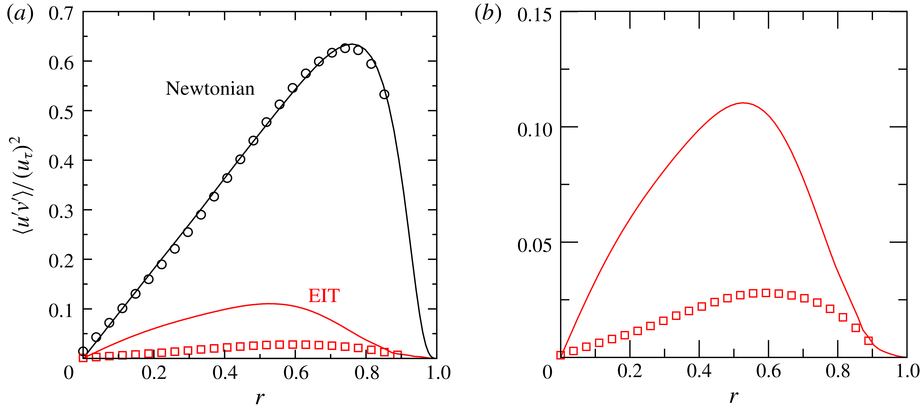
Figure 7(a) shows the time and area averaged Reynolds shear stress, $\langle -u^{\prime }v^{\prime }\rangle$ , for Newtonian turbulence and elasto-inertial turbulence in experiments (symbols) and simulations (solid lines). As seen, one of the prominent features of elasto-inertial turbulence as compared with Newtonian turbulence is its low Reynolds shear stress level. This is indicative that only a small fraction of the turbulent kinetic energy is produced by the conventional mechanisms of Newtonian turbulence, i.e. the self-sustaining cycle. Instead, turbulence here is primarily sustained by polymer stresses (Warholic et al. Reference Warholic, Massah and Hanratty1999). Note that while excellent agreement between simulations and experiments is obtained in the Newtonian case, the Reynolds shear stress level at EIT is larger by a factor of $3$ in the simulations (see figure 7 b). This may be a consequence of the artificial diffusion used in the simulations, which is known to mitigate the polymer stresses, thereby leading to larger levels of Reynolds shear stress. The maximum of $\langle -u^{\prime }v^{\prime }\rangle$ , which in the Newtonian case occurs near the wall, is located at an intermediate distance between the wall and the centreline, $r=0.52$ and $0.59$ in simulations and experiments, respectively. This is consistent with the thickening of the viscous buffer layer associated with high drag reduced flows (White et al. Reference White, Dubief and Klewicki2018). In contrast to Warholic et al. (Reference Warholic, Massah and Hanratty1999), where zero Reynolds shear stresses were measured at high drag reduction, our results show low but finite values, in line with other simulations of EIT (Samanta et al. Reference Samanta, Dubief, Holzner, Schäfer, Morozov, Wagner and Hof2013). There is, however, a substantial difference in $Re$ between our work (and other works on EIT) and that of Warholic et al. (Reference Warholic, Massah and Hanratty1999), and so a direct comparison between these results may not be appropriate.

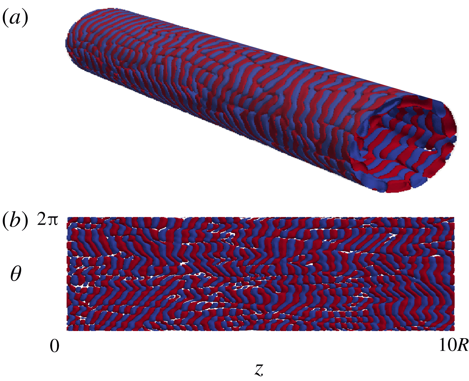
The topological structure of the new flow state is illustrated in figure 8 through isocontours of the second invariant of the velocity gradient tensor $\unicode[STIX]{x1D64C}$ . Note that this quantity has been chosen to facilitate comparison with other works on EIT (Samanta et al. Reference Samanta, Dubief, Holzner, Schäfer, Morozov, Wagner and Hof2013; Dubief et al. Reference Dubief, Terrapon and Soria2013). Regions of intense vorticity ( $\unicode[STIX]{x1D64C}>0$ , red) are found to alternate with strain-dominated regions ( $\unicode[STIX]{x1D64C}<0$ , blue) creating a chaotic pattern of elongated spanwise oriented structures aligned in streamwise direction. The vortices are localized in the near wall region and are essentially two-dimensional with rotation being in the $r{-}z$ plane. We note that this spatial arrangement of structures in the near wall region is very different from Newtonian type turbulence, where the dominant structures are oriented in the streamwise direction. This flow state reproduces two essential features of MDR: the drag reduction level associated with this state remains nearly constant as $Wi$ increases, and although the average friction factor ( $f\sim 0.0047$ ) is slightly below that corresponding to Virk’s asymptote ( $f=0.0051$ ), it is reasonably close to it. It should be noted that Virk’s asymptote is a fit of empirical data collected from different experiments. As such, it should be used as an estimate for the friction of the MDR state rather than as a categorical result. All these observations are consistent with previous reports of elasto-inertial turbulence in channel flow simulations (Samanta et al. Reference Samanta, Dubief, Holzner, Schäfer, Morozov, Wagner and Hof2013; Dubief et al. Reference Dubief, Terrapon and Soria2013).

Figure 8.

Isosurfaces of the second invariant of the velocity gradient tensor $\unicode[STIX]{x1D64C}=-0.005$ and $0.005$ illustrating the topological structure of elasto-inertial turbulence. (a) Shows a three-dimensional view of the pipe highlighting the near wall localization of the structures. (b) Shows the characteristic pattern, with alternating regions of rotational and extensional/compressional behaviour, in a cylindrical section $\unicode[STIX]{x1D703}{-}z$ at the wall. The state shown corresponds to a simulation conducted at $Wi=60$ for the LE case. The second invariant of the velocity gradient tensor is computed as $\unicode[STIX]{x1D64C}=(1/2)(\Vert \unicode[STIX]{x1D6FA}\Vert ^{2}-\Vert \unicode[STIX]{x1D6E4}\Vert ^{2})$ , where $\unicode[STIX]{x1D6FA}=(1/2)(\unicode[STIX]{x1D735}\boldsymbol{v}-\unicode[STIX]{x1D735}\boldsymbol{v}^{\text{T}})$ is the vorticity tensor and $\unicode[STIX]{x1D6E4}=(1/2)(\unicode[STIX]{x1D735}\boldsymbol{v}+\unicode[STIX]{x1D735}\boldsymbol{v}^{\text{T}})$ is the rate-of-strain tensor.

Figure 9.

(a) Shows the deviation of the streamwise velocity from the mean flow $u^{\prime }$ in a state of EIT for experiments conducted at $Re=3150$ . The velocity was measured using PIV in a pipe cross-section of nearly $6R$ in the axial direction. The image shown was obtained by assuming Taylor’s frozen hypothesis, i.e. turbulence is advected downstream quickly and changes in time are slow. (b,c) Show $u^{\prime }$ and $\unicode[STIX]{x1D64C}$ respectively for a simulation performed at $Re=3500$ and $Wi=30$ in a $40R$ long pipe. Two isocontours $u^{\prime }=\pm 0.1u_{max}^{\prime }$ and $\unicode[STIX]{x1D64C}=\pm 0.005$ were used in each case.

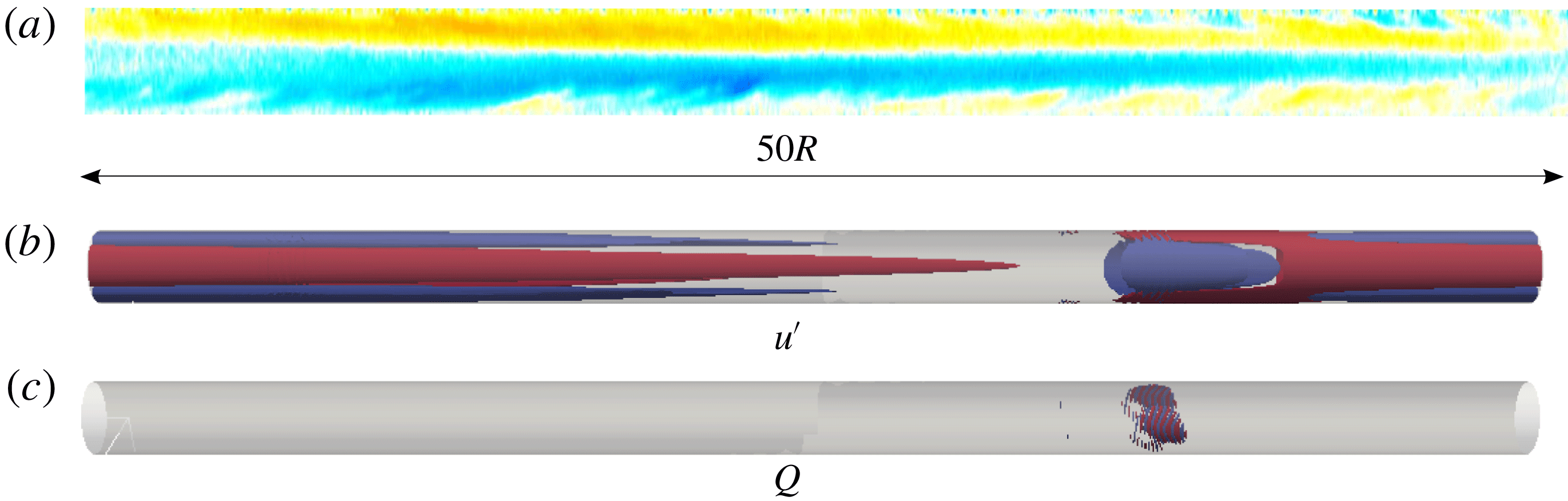
Figure 9(a) illustrates the typical flow structures of EIT in the experiments. It shows the streamwise velocity deviation with respect to the mean flow $u^{\prime }$ over a length of $50R$ . Note that in (a) the velocity was obtained from particle image velocimetry (PIV) in a section of nearly $6R$ in the axial direction and Taylor’s frozen turbulence hypothesis was then assumed to reconstruct the structures shown. As seen, the structure of EIT is clearly dominated by very elongated streaky structures aligned in the flow direction with a slight slope towards the centreline. The axial length of these structures is highly variable, ranging approximately from $50R$ to $200R$ , being more elongated near the instability onset. As polymer concentration increases, the structures become shorter and increasingly more chaotic but still preserve their characteristic inclination. Unlike in the simulations, vortical structures could not be resolved in the near wall region in the experiments. The vortical structures observed in the simulations are considerably weaker than Newtonian flow structures, which makes a detection in experiments difficult. In addition they are located close to the wall where the measurement accuracy is lower. In the simulations the problem is the opposite. Because of the Gauss–Lobatto–Chebyshev grid used in the radial direction the computational nodes are clustered near the wall, enabling an accurate resolution of the flow in this area. Nevertheless, the necessity of very dense grids in the streamwise direction to properly resolve the near wall structures makes it extremely costly to use axial domains sufficiently large as to capture the large scale structures observed in the experiments. A direct comparison of the structure of EIT between experiments and simulations is thus challenging. It is however tempting to investigate whether large scale structures can also be identified in simulations, and if their length approaches that of the structures in experiments as the computational domain is increased. To that extent, we have performed an additional simulation at $Wi=30$ using a pipe of $40R$ in streamwise direction. EIT could only be captured transiently in this simulation and after approximately $2500$ time units the flow went back to laminar. Nevertheless, some interesting dynamical aspects could be inferred from this simulation. As seen in figure 9(c), if the same threshold $\unicode[STIX]{x1D64C}=\pm 0.005$ as in figure 8 is used, the near wall vortices appear localized over a short region of nearly $2R$ in the streamwise direction. Large scale streamwise velocity structures (see figure 9(b)) seem to emerge from the area where the vortices are located and extend almost over the entire domain. These structures become thinner as they are followed downstream and take an arrow shape at the leading edge which closely resembles the inclination away from the wall observed in the experiments. This structural similarity between EIT in simulations and experiments suggests that the flow in both cases may be driven by the same instability. However, the precise dynamical relation between the small near wall structures and these elongated streaks still remains to be determined and will be the focus of a future investigation.