1. Introduction
Due to the significant demand on automated tasks, robot navigation plays an essential role in a plethora of industrial applications. The ability of autonomous robots to execute complex tasks and interact with their environment through highly sophisticated sensors and actuators induces their effective use in several industrial applications. Although navigation requirements differ from one environment to another, navigation is still built on three main pillars: mapping, localization, and path planning. Mapping is required to create a representation of the robot’s surroundings. Localization is needed to construct a cognition between the different robots and their global environment. By using the localization to monitor the position in the global map, the path (or waypoints) can be constructed and followed, accordingly. This is known as path planning, which is the third pillar of navigation.
The continuous recording availability of the sensor in a certain application is important for the localization performance since it measures the position in real time. Therefore, any loss in signal could lead to a false representation of the robot’s state, which affects the whole localization process. In other words, localization sensors or adopted methods need to have an alternative approach at instances where unexpected loss occurs to the robot position. Another significant factor is the cost of the sensor used since higher sensor accuracy comes at a higher cost. Moreover, higher accuracy could affect the range of the sensor, which leads to the use of multiple sensors to cover a certain environment. Therefore, range and accuracy are usually two opposite attributes [Reference Zhu, Yang, Wu and Liu1].
Many scientific and trigonometric approaches are utilized for localization estimation technologies. An example of that is time of arrival (TOA), which is based on measuring the time between a portable target and three least encompassing reference points, resulting in three circles; accordingly, the point at which these three circles cross is the object position. Although TOA requires a timestamped-synchronized flag, synchronization is partially dropped in the return time of flight strategy, and it is completely discarded within the time difference of arrival (TDOA) method to be supplanted by a time reference. Angle of arrival and direction of arrival are other approaches that utilize the crossing point of distinctive calculated lines from diverse sources (antennas) to calculate the position of the robot in an estimated radius that is resulted by the surrounding antennas. Triangulation is the method, from which, all the previous methodologies were derived [Reference Liu, Darabi, Banerjee and Liu2].
Localization techniques could be infrastructure dependent or infrastructure independent. The first category usually involves the wireless beacons which operate at different protocols. Wireless beacons depend on received signal strength indicator (RSSI), which indicates the difference between transmitted and received signal strengths. Thus, it does not require time involvement [Reference Alarifi, Al-Salman, Alsaleh, Alnafessah, Al-Hadhrami, Al-Ammar and Al-Khalifa3].
There are several wireless beacons applications, due to the wide bandwidth of the operating frequencies for each technology. Ultra-wideband (UWB) is an example of wireless beacons, which are robust to potential noises in the environment. However, UWB can still be sensitively susceptible to metallic objects in the environment, which can interfere with the original signal. Moreover, it is more expensive than other existing technologies [Reference Alarifi, Al-Salman, Alsaleh, Alnafessah, Al-Hadhrami, Al-Ammar and Al-Khalifa3], such as Wi-Fi, Bluetooth, or Radio-Frequency IDentification (RFID). All the previously mentioned technologies rely on the strength of the signal. However, Bluetooth uses the lowest power since it has the advantage to operate on “Bluetooth low power” (BLE) [4]. Although RFID is the most accurate technology among the former mentioned techniques, it lacks security since it can penetrate the obstacles or walls in the environment [Reference Alkhawaja, Jaradat and Romdhane5].
In infrastructure-independent techniques, the pre-setup of map (environment) is not needed, and the sensor is usually mounted on the robot itself, which makes it a better portable solution. An example of an infrastructure-independent technique is ultrasound, which is widely used in the medical field. Using reflected sound waves of a certain object, a depth image can be constructed. This is known as the B-scan technique, which helps in localizing and diagnosing a certain part of the body [Reference Hauff, Reinhardt and Foster6].
The use of inertial navigation systems (INSs) has increasingly gained attention in the last two decades due to their portability and ease of use. INS is a device that estimates acceleration, velocity, and position using the inertial measurement unit (IMU). IMUs consist of three (or four) main sensors, which are the accelerometer, the gyroscope, and the magnetometer. In some IMUs, the barometer is used to measure the altitude based on the pressure applied to the sensor. The accelerometer is used for measuring the acceleration to estimate the robot displacement, where the gyroscope is used to measure the angular speed in the three directions. Several companies utilize micro electro-mechanical systems to estimate steps count and distance taken by the user [Reference Lukianto, Hönniger and Sternberg7]. The technology is based on inertial measurements of the foot or the body movement using an integrated IMU in portable devices [Reference Nilsson, Gupta and Handel8]. INS can be fused with other technology such as visual sensors [Reference Karamat, Lins, Givigi and Noureldin9] or wireless beacons (Wi-Fi, Bluetooth, RFID, etc.) [Reference Seitz, Vaupel, Meyer, Boronat and Thielecke10] to estimate the initial position, give more accurate results in a dynamic operating environment, and compensate for the drift errors that the IMUs suffer from. Ground-based robots use wheel encoders to ultimately estimate robot position and velocity to generate odometry [11].
The use of visual and infrared sensors is another example of an infrastructure-independent technique. By using a constructed depth image resulting from the reflections of the infrared light grid, the distances from each point of the environment to the sensor frame can be estimated. The projections on the environment are continuous at a certain frame rate, which is different from one sensor to another. However, the frame rate is usually dropped by the algorithm used to extract the features from the depth image to localize the sensor and create a cognition between the robot and its surroundings. This causes the frame rate to drop significantly as is the case for the real-time appearance-based mapping (RTABMAP), which has a maximum frame rate of 1 Hz [Reference Labbe and Michaud12]. Moreover, the rotations of the frame caused by the robot could dramatically reduce the number of features in the depth image, which results in a failure in the localization step, which affects the navigation process. Therefore, the fusion between the previously mentioned approaches is needed to reduce the dependency on a certain technique and compensate for the limitations of the used sensors.
The use of neural networks for fusing multiple sensors has been an interesting field in the last two decades due to the flexibility that neural networks provide. Many RSSI-related pieces of research had used neural network algorithms to improve their indoor navigation systems.
Many researchers are utilizing multiple sensor fusion techniques to reduce the overall localization error and have a better availability and reliability of the sensor readings at all instances, therefore accounting for shortcomings or high delays of a certain sensor. An example of that is the use of the depth camera, in complicated environments, where many pixels need to be processed in real time. In ref. [Reference Song, Choi and Kim13], an adaptive color-based particle filter was used to fuse the reading of an RGB-D camera and a Light Detection and Ranging (LiDAR).
The authors of ref. [Reference Al-Mutib and Sabtio14] have used the RFID technology with the assistance of backpropagation artificial neural networks (BPANN). The idea was to classify at least two maximum points through RSSI to acquire the location until one maximum RFID measurement drops, which triggers the algorithm to rescan for new RFID tags registration. The BPANN advantage is to reduce the number of RFID tags needed for the localization process while giving a reduced error simultaneously. RSSI localization-related applications are increasingly receiving interest to be assisted by neural networks due to the uncertainties that are involved in the received signals [Reference Shareef, Zhu and Musavi15, Reference Abdelgawad16]. The authors of ref. [Reference Shareef, Zhu and Musavi15] used multiple methods to compare different neural network methods. Another approach was used in ref. [Reference Abdelgawad16], which utilizes RFID tags to estimate TDOA to predict the next location using the Kalman filter (KF). KF is a powerful tool to fuse different inputs to have a prediction for the next state that would contribute to the next measurement [Reference Malyavej, Kumkeaw and Aorpimai17]. The different versions of KF (e.g., extended KF/unscented KF) provide a powerful tool to integrate several types of signals coming from different signals [Reference Malyavej, Kumkeaw and Aorpimai17–Reference Corrales, Candelas and Torres19]. In ref. [Reference Yousuf and Kadri20], authors used the KF to fuse GPS-INS sensors, and GPS odometry in outdoors environments. For the case of indoor environment, when the GPS fails to receive signals, a neural network is used to testify the INS and the odometry sensors readings. This was augmented by an implantation of a fuzzy logic system for the potential slippery of the wheels.
Neural networks and other fusion techniques are also helpful in enhancing the localization for a GPS/IMU navigation. In refs. [Reference Saadeddin, Abdel-Hafez, Jaradat and Jarrah21] and [Reference Jaradat and Abdel-Hafez22], an adaptive neuro-fuzzy inference system was used to compensate for the potential GPS signal unavailability. A variable delay was introduced as an input to the system, to account for the difference in the sampling rates between the IMU and the GPS signals. By subtracting the estimated error at each iteration, the method gives the updated velocity and position information. Similarly, the authors in ref. [Reference Jaradat and Abdel-Hafez23] have used the delay between the GPS measurements as an input to the used non-linear autoregressive intelligent fusion between the IMU measurements and the GPS ones, to account for GPS outages using the non-linear system. The use of IMU/GPS, vision sensors, and their fusion through multi-layer perceptron neural networks methods are compared in ref. [Reference Ragab, Ragab, Givigi and Noureldin24]. Although the use of vision sensors showed a slight reduction in the error, the use of neural networks fusion has significantly reduced the error, ultimately.
The main objective of this work is to enhance the process of navigation, by enhancing the localization process and developing a low-cost depth/IMU intelligent sensor fusion approach. This is performed by fusing the depth camera collected pose values with the IMU-based pose data, using a feedforward cascade correlation network (CCN). Since the IMU fails to be a robust sensor to be used for posing localization, the depth camera can be used to extract pose information and result in a more accurate localization. However, the depth camera could lose frames due to assorted reasons during this mission. The proposed algorithm would compensate for the losses in signal availability that might happen to the depth camera while localizing by correcting the drift accompanied with the use of the IMU sensor, via the depth camera sensor measurements. This approach has the advantage of integrating the high frequency of the IMU sensor measurements and the accuracy of the depth camera measurements.
CCN is a methodology to build an optimized topology of the neural network layers, which best fits the application. CCN is usually used in stock market research [Reference Abdou, Tsafack, Ntim and Baker25] due to its ability to alter and build on the previous network as time progresses. This feature is helpful in predicting stock prices since the networks can still adapt continuously to the changing stock profiles [Reference Velusamy and Amalraj26] or to the sudden financial distresses [Reference Abid and Zouari27]. CCN is also used in biomedical applications, for example, breast cancer diagnosis [Reference Nachev, Hogan and Stoyanov28] due to their quick response which makes them sensitive to insignificant changes without the need to determine the number of hidden layers.
The use of CCN in localization was adopted in research with promising results. In ref. [Reference Chen, Lin and Lin29], the authors used five CCN models to calculate the position of an object using RFID tags through RSSI. Similarly, CCN was used in INS/GPS systems [Reference Chiang, Noureldin and El-Sheimy30] and was compared to artificial neural network (ANN) showing that CCN outperforms ANN by having less execution time and a lower error. Based on the mentioned advantages, an intelligent fusion algorithm based on CCN is selected to integrate the depth camera sensor with the IMU sensor for mobile robot localization and navigation.
This paper will be organized as follows: the next section introduces the methods and materials used for the localization of the robot. The results and their discussion are presented in Section 3. Finally, Section 4 presents the conclusion highlighting the main contribution of this paper.
2. The process of localization
Although the approaches of localization are many, this work will focus on using an affordable portable sensor to be mounted on the robot for localization, developing a low-cost depth/IMU intelligent sensor fusion approach. Using a predefined map, the optimal path is constructed to help the robot reach its destination. Moreover, to ensure accuracy, localization needs to be continuously available as the robot is navigating to the destination.
This section first introduces the different methods of localization used by the different sensors, and then the fusion localization method follows using CCN neural network.
2.1. Mobile robot odometry: Kinematic model
The mobile robot platform used in this research is Kobuki differential wheeled robot platform [Reference Siegwart, Nourbakhsh and Scaramuzza31]. As a non-holonomic mobile robot, the Kobuki has its two-dimensional model, which gives the position and orientation of the local frame, with respect to the global one, as shown in Fig. 1 [Reference Siegwart, Nourbakhsh and Scaramuzza31].
The local reference frame and global reference frame.

The global generalized velocity vector
 $\dot{G}$
shown in Eq. (1) includes three variables,
 $X_{\text{odom}}$
,
 $Y_{\text{odom}}$
(the state in 2D frame), and
 $\theta _{\text{odom}}$
(heading),
 \begin{equation}\dot{G}=\left(\begin{array}{c} \dot{X}_{\text{odom}}\\[4pt] \dot{Y}_{\text{odom}}\\[4pt] \dot{\theta }_{\text{odom}} \end{array}\right)\end{equation}
where the local frame velocity matrix (Eq. 2),
 \begin{equation}\dot{P}=\left(\begin{array}{c} \dfrac{r(\dot{{\varnothing }}_{R}+\dot{{\varnothing }}_{L})}{2}\\[7pt] 0\\[4pt]\dfrac{r(\dot{{\varnothing }}_{R}-\dot{{\varnothing }}_{L})}{2l} \end{array}\right)\end{equation}
where
 $r$
is the radius of the Kobuki robot wheel which equals 0.0352 m,
 $l$
is the distance between the two wheels which equals 0.21 m, and
 ${\varnothing }$
represents the robot wheel angle for right and left wheels.
In order to relate the robot’s local frame to the global frame, a rotation matrix needs to be introduced (
 $R$
) as shown in Eq. (3).
 \begin{equation}R=\left(\begin{array}{c@{\quad}c@{\quad}c} \cos\!\left(\theta _{\text{odom}}\right) & -\sin\! \left(\theta _{\text{odom}}\right) & 0\\[4pt] \sin\! \left(\theta _{\text{odom}}\right) & \cos\!\left(\theta _{\text{odom}}\right) & 0\\[4pt] 0 & 0 & 1 \end{array}\right)\end{equation}
The rotation matrix calculates the global frame state matrix in relation to the local frame state matrix. The relationship between the local frame and the global frame is shown in Eq. (4).
 \begin{equation}\dot{G}=R\dot{P}\end{equation}
To track the position and orientation of the robot in the global reference frame, one must measure the local change of position and orientation of the robot and use the
 $R$
matrix to obtain the needed information. This process is usually referred to as dead reckoning, which consists of estimating the value of the position and orientation using the earlier value and adding the current changes.
Diverse types of sensors provide different types of information about the position and orientation of the robot. IMUs and embarked depth cameras sensors, for example, provide local pose information individually, which needs to be converted to the global frame that represents the robot global state.
In the rest of this section, the different sensors used in this work are presented along with the methodology needed to extract the pose information related to the above model.
2.2. Localization using IMU sensor
Accelerometers and gyroscopes sensors are basic components in the IMU unit, which work together to measure the three accelerations and the angular velocities, along the three axes in space.
Typically, IMUs have one accelerometer, gyro, and magnetometer per axis, for each of the three axes: pitch, roll, and yaw. These sensors detect the motion and output a signal, which could be an acceleration from the accelerometer sensors or an angular velocity from the gyroscope sensors.
To enhance the performance of the accelerometer, the jerk has been taken into consideration to remove the abrupt changes of velocity, as in ref. [Reference Ibrahim and Moselhi32]. The use of jerk requires four consecutive accelerations readings in order to filter out the noises or unwanted readings as in Eqs. (5)–(7).
 \begin{equation}J_{1}=\frac{\text{acc}_{2}-\text{acc}_{1}}{dt}\end{equation}
 \begin{equation}J_{2}=\frac{\text{acc}_{4}-\text{acc}_{3}}{dt}\end{equation}
 \begin{equation}A_{t}=\frac{J_{1}-J_{2}}{2}dt\end{equation}
where
 $\text{ac}\text{c}_{i}$
and
 $J_{i}$
are the measured acceleration and the jerk values of the ith iteration, respectively. Then the local acceleration
 $A_{t}$
is estimated according to Eq. (7). Therefore, the acceleration is taken every four iterations. These equations will be applied to the three directions so that it gives the filtered acceleration values in the three local axes. The use of jerk calculations will automatically detect the gravity component and remove it at any initial state. Moreover, it will continue to cancel gravity at the next states as shown in ref. [Reference Ibrahim and Moselhi32]. A rotation matrix is used to convert the IMU measured accelerations to the global axes [Reference Premerlani and Bizard33, Reference Khan, Clark, Woodward and Lindeman34]. Eq. (8) shows the rotation matrix that needs to be applied, followed by Eq. (9) that shows the global acceleration
 $\boldsymbol{A}_{t}$
. As the IMU measurements would always be relative to its initial position (local position), the differences in the angles can be used to estimate the position in the global frame. Consequently, the global acceleration values will be integrated using Eqs. (10) and (11), resulting in the 3D position in the global frame.
 \begin{equation}\boldsymbol{R}_{\textbf{IMU}}=\left(\begin{array}{c@{\quad}c@{\quad}c} {\cos }\boldsymbol{\theta }{\cos }\boldsymbol{\psi } & {\sin }\boldsymbol{\varnothing }{\sin }\boldsymbol{\theta }{\cos }\boldsymbol{\psi }-{\cos }\boldsymbol{\varnothing }{\sin }\boldsymbol{\psi } & {\cos }\boldsymbol{\varnothing }{\sin }\boldsymbol{\theta }{\cos }\boldsymbol{\psi }+{\sin }\boldsymbol{\varnothing }{\sin }\boldsymbol{\psi }\\[4pt] {\cos }\boldsymbol{\theta }{\sin }\boldsymbol{\psi } & {\sin }\boldsymbol{\varnothing }{\sin }\boldsymbol{\theta }{\sin }\boldsymbol{\psi }+{\cos }\boldsymbol{\varnothing }{\cos }\boldsymbol{\psi } & {\cos }\boldsymbol{\varnothing }{\sin }\boldsymbol{\theta }{\sin }\boldsymbol{\psi }-{\sin }\boldsymbol{\varnothing }{\cos }\boldsymbol{\psi }\\[4pt] -{\sin }\boldsymbol{\theta } & {\sin }\boldsymbol{\varnothing }{\cos }\boldsymbol{\theta } & {\cos }\boldsymbol{\varnothing }{\cos }\boldsymbol{\theta } \end{array}\right)\end{equation}
 \begin{equation}\boldsymbol{A}_{t}=\left[\begin{array}{c} \boldsymbol{A}_{{\boldsymbol{x}_{t}}}\\[4pt] \boldsymbol{A}_{{\boldsymbol{y}_{t}}}\\[4pt] \boldsymbol{A}_{{\boldsymbol{z}_{t}}} \end{array}\right]=\boldsymbol{R}_{\textbf{IMU}}A_{t}\end{equation}
 \begin{equation}\boldsymbol{v}_{k}=\boldsymbol{A}_{t}dt+\boldsymbol{v}_{k-1}\end{equation}
 \begin{equation}\boldsymbol{P}_{\text{k}}=\boldsymbol{v}_{k}dt+\boldsymbol{P}_{k-1}\end{equation}
where
 $\theta, \phi, \psi$
represent the rotation angles in the three dimensions (yaw, pitch, and roll), the vector
 $\boldsymbol{v}_{k}$
represents the current velocity, and the vector
 $\boldsymbol{P}_{k}$
represents the current position which includes
 $\boldsymbol{X}_{\textbf{IMU}}$
,
 $\boldsymbol{Y}_{\textbf{IMU}}$
, and
 $\boldsymbol{Z}_{\textbf{IMU}}$
. Some IMUs are equipped with a pressure sensor to measure the altitude above the sea level using Eq. (12) [Reference Ibrahim and Moselhi32].
 \begin{equation}\text{Altitude}_{\text{barometer}}=\text{C}_{1}\left(1-\left(\frac{P}{P_{0}}\right)^{\frac{1}{\text{C}_{2}}}\right)\end{equation}
where
 $C_{1}$
and
 $C_{2}$
are non-dimensional constants and equal to 44,330 and 5.255, respectively, at 15°C, while
 $P$
is the measured pressure and
 $P_{0}$
is the pressure at the sea level (1013.25 hPa). An additional improvement that can be used is the magnetometer sensor in the IMU.
2.3. Depth-based localization
The chosen depth camera (Intel d435) provides two techniques of depth-based localization, which makes it less vulnerable to noises and vibrations. The first technique relies on the idea of “stereo camera,” which tries to imitate the human eyes, by utilizing the focal lengths of two adjacent lenses. As shown in Fig. 2, using triangulation, the distance from the camera reference to the object is calculated. Therefore, each point seen by the lenses can be considered as a feature to be used in the localization process. Eqs. (13)–(16) explain the stereo localization process [Reference Kang, Webb, Zitnick and Kanade35].
 \begin{equation}\frac{f}{{z}}=\frac{x_{1}-x_{2}}{b}\end{equation}
 \begin{equation}{z}=f\frac{b}{x_{1}-x_{2}}\end{equation}
 \begin{equation}x=x_{1}\frac{{z}}{f}\end{equation}
where
 $f$
is the focal length,
 $z$
is the depth distance from the camera to the object,
 $x_{1}$
and
 $x_{2}$
are the horizontal distances from both of the cameras to the object, d is the disparity,
 $b$
is the fixed distance between the two cameras (baseline), and
 $x$
is the horizontal distance from the camera frame to the object. Similarly, the vertical distance
 $y$
in Eq. (16) is formulated. However, for this application, the robot performs a planar motion, hence
 $y$
is constant.
 \begin{equation}y=y_{1}\frac{{z}}{f}\end{equation}
The position can be estimated by iterative closest point algorithm [Reference Ruan36], which relates two point-clouds by a rotation and translation matrix that can be calculated using least mean squares minimization. Moreover, the rotational angles (pitch, roll, and yaw) can be computed from the current plane orientation (i.e.,
 $\Phi =\tan ^{-1} (z/x)$
is used for the roll angle) [Reference Sappa, Dornaika, Ponsa, Gerónimo and López37]. Hence, the pose is estimated.
Path resulted from the selected points according to the 2D cost map.

Path resulted from the selected points according to the 2D cost map.

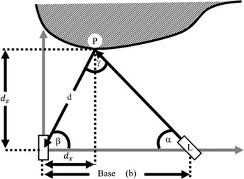
On the other hand, an assistive algorithm is used along with the stereo camera to ensure more reliability, known as “structured light technology” [Reference Gupta, Agrawal, Veeraraghavan and Narasimhan38]. This technique uses a cloud of infrared lights projected on the map and received by an infrared receiver (IR) as shown in Fig. 3. Using triangulation, the distance to a certain point of projection can be calculated as shown in Eqs. (17)–(20).
 \begin{equation}\frac{d}{\sin\! \left(\alpha \right)}=\frac{b}{\sin\! \left(\gamma \right)}\end{equation}
Since
 $\sin \gamma =\sin\! (\pi -\gamma )$
, where
 $\alpha +\beta =\pi -\gamma$
 \begin{equation}d=b\frac{\sin\! \left(\alpha \right)}{\sin\! (\alpha +\beta )}\end{equation}
accordingly,
 \begin{equation}d_{x}=d \cos (\beta )\end{equation}
 \begin{equation}d_{z}=d \sin\! (\beta )\end{equation}
The selected method of depth localization in Intel d435 performs localization by taking features from the environment by the fusion of its stereo cameras and IR. These features are produced by Harris corner detection [39] with adaptive non-maximum suppression [Reference Liu, Huang and Wang40], and then the scale-invariant feature transform algorithm was used to create a 128-dimensional descriptor for every feature [Reference Lowe41, 42]. Therefore, these features will be continuously compared to previously saved features (using sum of squared distances ratio SSD Ratio) to detect closed-loop (viewing loop) and enhance the localization process. This method is known as RTABMAP [Reference Labbé and Michaud43]. RTABMAP uses ORB-SLAM to keep track of the location. ORB-SLAM, in turn, is based on “stereo camera” and “structured light technology” principles [Reference Ruan36]. The camera frames will help construct the map; in turn, the depth images will be used to localize the camera with respect to its environment. Accordingly, the 2D results from the camera are longitude and latitude values.
Figure 3 shows the depth camera from a top view, resulting in a two-dimensional frame. However, it is worth noting that this is a dense representation which incorporates a third dimensional component.
Since the use of the camera and the RTABMAP module yield the pose of the camera, one needs to apply another transformation to obtain the pose of the Kobuki, which is the global frame. This transformation can be represented by a homogeneous matrix
 $\boldsymbol{H}$
given by:
 \begin{equation}\boldsymbol{H}=\left[\begin{array}{c@{\quad}c} \boldsymbol{R} & \boldsymbol{T}\\[4pt] \textbf{0}_{(\textbf{1}\times \textbf{3})} & \textbf{1} \end{array}\right]\end{equation}
where
 $\boldsymbol{R}$
is the rotation matrix and
 $\boldsymbol{T}$
is the translation vector [44]. With reference to the experimental setup shown in Fig. 13, the rotational matrix
 $\boldsymbol{R}=\left[\begin{array}{c@{\quad}c@{\quad}c} 0 & 0 & 1\\[4pt] 1 & 0 & 0\\[4pt] 0 & 1 & 0 \end{array}\right]$
and the translational matrix
 $\boldsymbol{T}=\left[\begin{array}{c} 0\\[4pt] 0\\[4pt] h=-0.2763 \end{array}\right]$
, since the camera is fixed at the center of the Kobuki with a fixed measured height of 27.63 cm. These quantities are fixed throughout the missions to relate the local camera reference frame to the global reference of the Kobuki.
Points projected and received by the sensor vary depending on the environment and the graphical processing unit (GPU) used to operate the Intel d435 camera. The more distinctive is the environment, the more features are in the frame. Moreover, the fastest frequency at which the camera can operate is 1 Hz, this frequency is set as a default setting. However, this frequency can be reduced if a low-end GPU is used. Lower frequencies cause fewer features in the frame, which reduces the quality of the localization accordingly.
2.4. Depth/IMU intelligent sensor fusion framework
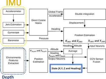
The above sensors are mounted on a Kobuki mobile robot developing a low-cost depth/IMU intelligent sensor fusion approach. In this approach, the slow depth camera localization and the fast-inaccurate IMU localization are fused based on a modified CCN neural network approach as shown in Fig. 4 [Reference Chiang, Noureldin and El-Sheimy30, Reference Malleswaran, Vaidehi and Jebarsi45–Reference Malleswaran, Vaidehi, Saravanaselvan and Mohankumar47]. Initially, the IMU sensor provides the robot absolute position based on Eqs. (5)–(9), and this solution is generated based on the “Direct Cosine Matrix,” correction of the gravity, and “Double Integration” blocks [Reference Bikonis and Demkowicz48], providing the globalized IMU 2D frame measurements. The performed localization process by the IMU sensors is completed by the “Position Estimation” block; the outputs
 $\boldsymbol{X}_{\textbf{IMU}} \text{and} \boldsymbol{Y}_{\textbf{IMU}}$
are fed to the CNN neural network as inputs. IMU sensors output is normalized in order to provide flexibility and scalability for other paths. On the other hand, the depth camera extracts the features in the frame, to generate the global frame for the camera and estimate
 $\boldsymbol{P}_{\text{depth}}$
using RTABMAP python library. However, the depth frame 2D pose is considered as neural network target outputs. The collected heading (
 $\theta _{\text{IMU}}$
and
 $\theta _{\text{Depth}}$
) and altitude (
 $Z_{\text{IMU}}$
and
 $Z_{\text{Depth}}$
) from both sensors are averaged and are fed to the final state estimation block in Fig. 4. The averaging of the heading and the altitude is to minimize the small drift in the gyroscope in short missions [Reference Li, Gao, Meng, Wang and Guan49], and the absence of it in the barometer [Reference Mummadi, Leo, Verma, Kasireddy, Scholl, Kempfle and Laerhoven50], respectively. Moreover, drift in the gyroscope can be corrected with the help of the accelerometer, thus yielding more reliable results.
The localization framework using IMU and depth sensor.

2.5. Localization using cascade correlation neural network fusion
Although the camera depth sensor is a reliable source and its accuracy is higher than the IMU accuracy [Reference Lukianto, Hönniger and Sternberg7], it is not as fast as the IMU sensors, and it does not work in all conditions. The camera depth sensor can lose availability when it is too close to the wall, or when a severe swerve occurs by the robot. Therefore, fusing both sensors would enhance the localization process and would decrease the dependency on a certain sensor for localization.
Filters such as KF have several limitations such as the need of knowing the covariance values and the statistical properties in advance. Several limitations of KF were discussed in refs. [Reference Grewal and Andrews51–Reference Mohammed57]. Thus, neural networks are superior, since they do not require the model of the system, making them easily implementable on any hardware.
Determining the best topology when applying neural network creates a challenge when designing the ANN, which also includes the hidden neurons and hidden layers in the network. Several ways were discussed to determine the best size (hidden neurons) and depth (hidden layers) for the neural networks in refs. [Reference Borkowf58] and [Reference Bishop59], which indicate that the size and depth are mainly dependent on the applications itself.
The chosen fusion method is a constructive neural network since it can adjust its layers based on the needs. It starts constructing the layers one by one, while continuously checking if the number of layers is sufficient.
Several methods for constructive neural networks were proposed in refs. [Reference Chiang, Noureldin and El-Sheimy30, Reference Malleswaran, Vaidehi and Jebarsi45–Reference Malleswaran, Vaidehi, Saravanaselvan and Mohankumar47, 60]. The CCN [Reference Nachev, Hogan and Stoyanov28] was selected due to the aforementioned advantages and uses.
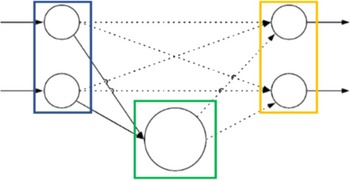
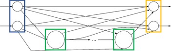
The topology of the CCN starts as shown in Fig. 5, followed by an explanation in Table I. The weights linking the input neurons to the output ones are started to be trained. This topology will be extended adaptively based on the application needs. As shown in Fig. 4, the input neurons receive the IMU-based pose data in the global frame (
 $X_{\text{IMU}}$
and
 $Y_{\text{IMU}}$
). The output neurons provide the estimated corrected IMU measurements, while the measured pose values from the depth camera solution (
 $X_{\text{Depth}}$
and
 $Y_{\text{Depth}}$
) are used as the target values for training.
The explanation of the CCN topology shown in this section.

Initial topology for CCN (no hidden layers).

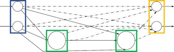
Second phase of CCN when adding a hidden layer.

The model keeps on building layers based on the initial topology until no further improvement can be made. The input data are trained through the Quickprop algorithm which does not require any backpropagation to adjust the weights [Reference Fahlman61]. Quickprop is relatively fast and simple compared to other algorithms [Reference Bishop59].
The next phase is to recruit a new pool of candidate neurons as shown in Fig. 6 by declaring initial weights. The candidate neurons are firstly trained based on their connections to input neurons, while the connections to the output neurons have not been made yet. The training is done to ultimately maximize the correlation among all connections going from the candidate neurons to the output neurons. Thus, a pseudo connection is made to deliver information about the residual error that was initially randomized, resulting in a maximization of the correlation in the connections from the candidate neurons and the residual error at the output neurons [Reference Chiang, Noureldin and El-Sheimy30]. Eq. (22) represents the maximization formula; its parameters are explained in Table II.
 \begin{equation}S=\sum _{o}\left| \sum _{p}(V_{p}-\overline{V})(E_{p,o}-\overline{E_{o}})\right|\end{equation}
Maximizing
 $S$
can be done through differentiation which uses the Quickprop algorithm to adjust concerning weights. Afterwards, the winner neurons layer based on the incoming weights will be frozen, resulting in the insertion of the winner layer into the active network once the training is completed. This engages the second step of recruitment, in which the weights of the connections from the hidden neutrons to the output neurons become adjustable and start to be trained, through a sigmoidal activation function. In addition, the input neurons connections to the output neurons are retrained as shown in Fig. 7.
Parameters of Eq. (22).

Winner neurons (WN) trained to match output neurons.

When another layer of hidden neurons is added, the entire process starts again as shown in Figs. 8 and 9. This process repeats itself and the layers of hidden neurons are added until no further improvement can be done, or the number of training passes reaches its maximum. Finally, the network can be represented with (n) hidden neurons and layers modified in a feedforwarded manner as shown in Fig. 10.
Third phase of CCN when adding the second hidden layer.

The second set of (WN) are trained to match the output neurons.

Full architecture with N hidden layers (neurons).

To reduce the complex interactions between the hidden neurons, the backpropagation is replaced by a feedforward algorithm. Moreover, the feedforward algorithm can always be incremented; hence, the trained layers will stay and will not need to be retrained again as shown in Fig. 9. CCN topology is determined automatically depending on the application complexity, so the need of performing additional trials to re-decide the hidden neurons and hidden layers does not exist.
Finally, the trained network is used in the fusion process. Based on the average error histogram among 60%, 70%, 80%, 90%, and 100% training data, 80% was observed to be the best percentage among the other percentages. The final structure of the CCN has 12 layers where each hidden layer has two neurons while being cascaded until the last layer.
3. Experimental setup and framework
3.1. Mapping and path-planning algorithms
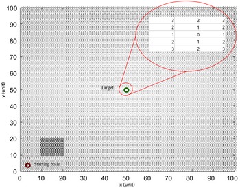
With the prior knowledge of an indoor environment, a grid-cost map can be introduced based on the starting node and the goal node. A node-based algorithm such as A* can be used to give the path in real time, to generate the path and the associated waypoints. Part of the path-planning algorithm is obstacle avoidance, which involves using a pre-existing map. Therefore, obstacles should have an infinite cost to force the algorithm to avoid the nodes of the obstacle in the cost map. A 2D grid-cost map is shown in Fig. 11.
The black box in Fig. 11 represents the change in the values of the cost map to infinity where the obstacle exists. Then, the different obstacles of the map can be added similarly. A* is used due to its lower computational cost and faster path planning. The grid is based on the location of the starting node and the ending one in addition to the distance between them, which will define the step size for the grid-cost map.
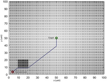
The shown grid-cost map in Fig. 11 creates the waypoints while considering the need of changing the heading. In other words, since the used robot is non-holonomic, the rotation of the robot will be considered as an extra waypoint. In order to generate a more efficient navigational path and reduce the number of waypoints, the waypoints at which the orientation is changing are selected.
The generated waypoints of the previous path.

2D Grid cost showing the cost (intensity of the color) with the presence of an obstacle.

An illustrative example is shown in Fig. 12, with a reduced number of points on the map for faster convergence. The resolution of the provided grid depends mainly on object sizes, shapes in the environment, and size of the environment. Table III shows the generated waypoints, which will be fed to the robot navigation program to track. The epoch number is just a representation of the time at each waypoint passage. The axes in Figs. 11 and 12 are unitless as they represent the steps in the map.
Path resulted from the selected points according to the 2D cost map.

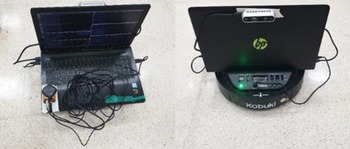
Experimental setup.

3.2. Used framework and platform
The framework of all the used sensors and actuators is the robotic operating system (ROS) [62]. The main advantage of ROS is that it provides a domain for all the sensors and actuators to communicate with each other in different patterns, distinct types, and various locations. The mobile robot used is Kobuki. The Kobuki robot is a ROS-enabled robot, which makes it integrable with a variety of sensors and other actuators.
The used IMU is the XSens Mti-G-710 GNSS. It is a 10 Degrees of Freedom IMU that consists of a three-axis accelerometer, a three-axis gyroscope, a three-axis magnetometer, and a barometer. The magnetometer is not used due to disturbances that may arise in the environment. The GPS mounted on the XSens- IMU is automatically enabled when there is an available signal in an outdoor environment. The use of the GPS/IMU, in this work, is to compare the indoor environment result to the outdoor one using a commercial off-the-shelf available solution [Reference Jaradat and Abdel-Hafez22]. This is done through extended KF fusion between the IMU and GPS in the XSens Module as in ref. [Reference Bikonis and Demkowicz48]. The XSens solution (IMU/GPS fusion) is used as a reference in the outdoor environment. On the other hand, Kobuki mobile robot platform is utilizing the odometry solution based on its internal IMU sensor and wheels’ encoders to provide the localization measurements for indoor environment. To verify the accuracy of the Kobuki odometry solution, a test has been conducted to follow a certain path. The conducted test is based on the validation of the non-holonomic robot model presented in ref. [Reference Renawi, Jaradat and Abdel-Hafez63]. During the test, actual waypoints in a U-shaped path were compared to the desired waypoints put on the floor. The mean error in robot position for X and Y axis is 0.011 and 0.033 m, respectively.
The recorded path by depth camera, Kobuki odometry, GPS, and IMU.

Many options are available in the market for depth sensors [Reference Alkhawaja, Jaradat and Romdhane5]; however, the chosen depth sensor was the Intel d435 depth camera. The mentioned camera was chosen based on two main reasons. First, the weight of the Intel d435 is 71 g which is low compared to the other existing depth cameras. Second, unlike several depth cameras and IR sensors, Intel d435 has a standalone USB-C port that is responsible for power and data transfer. USB-C port is capable of providing high power without compromising the speed of the data transfer. Other sensors might need a battery which increases the weight of the whole platform. Intel d435 is a ROS-enabled camera; as indicated in Fig. 4, the depth camera solution provides the estimated position of the robot based on fusion of the collected depth measurements by the camera, and more information about the Kobuki robot can be found at ref. [64]. Figure 13 shows all the sensors (IMU, GPS, and depth camera) and the laptop mounted on the Kobuki robot.
3.3. Control
The Kobuki mobile robot is a non-holonomic platform, where the wheel odometry (from the encoder) is linked to its heading. Wheels’ encoders are used to sense its movement in the X and Y axes. However, the robot wheels motor can only actuate in its local X axis. Therefore, the controller is controlling the robot linear velocity along the X axis, only. Mainly a proportional integral (PI) controller is used to control the speed of the robot as in Eq. (23).
 \begin{equation}v=K_{p}e_{v}+K_{i}\int _{0}^{T}e_{v} dt\end{equation}
where
 $e_{v}$
is the error in the linear speed. The gains of the PI controller were obtained using the process reaction curve through Cohen–Coon method [Reference Joseph65] (
 $K_{p}=9.465, K_{i}=0.642$
). The accepted error range was 0.01 m before moving onto the next waypoint.
Once the waypoints are fed to the user-defined navigation program, the robot divides the waypoints into two main categories (linear and twist). The linear category is for the robot linear movement considering that the orientation has been achieved already. The twist category is for the robot rotation to adjust and achieve the needed orientation.
4. Results
In this section, multiple paths are applied on the proposed localization algorithm to validate its robustness and adaptability. Based on the given framework in Fig. 4, CNN utilizes the depth camera solution pose values to provide the estimated location based on the collected IMU measurements which represent the IMU-based pose data. For the indoor environment, the Kobuki robot odometry solution is used as a reference for comparison.
4.1. Indoor environment comparison of the used sensors
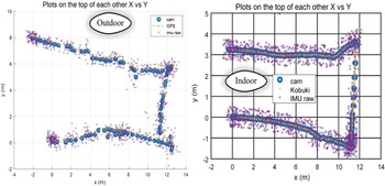
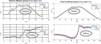
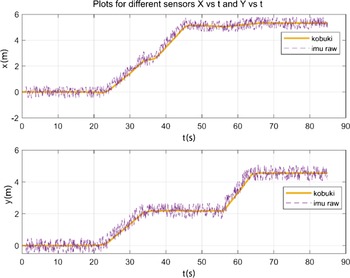
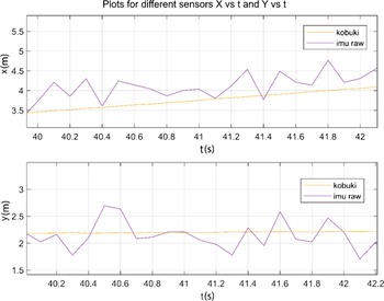
Initially, this test was conducted as a verification step, to compare the performance of different sensors used in the indoor environment. The pose data of the different sensors are shown in Figs. 14–17, comparatively. First, the pose data are shown on top of each other. Then, the pose data are plotted with respect to time. Table IV demonstrates a remarkably close performance of the depth camera sensor for the outdoor and indoor missions, while using the same path. This proves the robustness to light conditions from the camera perspective in both environments. Note that, the drift of the IMU resets at every observation of the depth camera. IMU calculated pose data based on the acceleration measurements is indicated as “IMU raw,” with no CCN correction.
x and y values with respect to time.

Zoomed view on recorded x and y values for the outdoor test.

As shown in Table IV, the error difference between the indoor test and the outdoor test is independent of the environment type since the used sensors are independent.
The depth camera average errors for different environments.

Zoomed view on recorded x and y values for the indoor test.

4.2. Using CNN
In this section, the training and testing are done in an indoor environment. First, an S-shaped path is used for the training step, while setting the training percentage to 80%, since it was the optimum value while avoiding overfitting. Second, another path is used by setting a starting point and a destination. The path (waypoints) was generated autonomously, while having an obstacle present in the map (similar to Fig. 12).
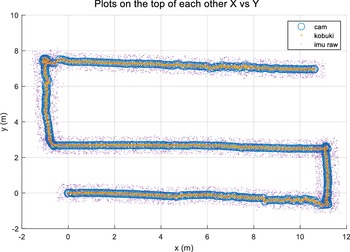
Collected measurements from following the path by the three sensors.

X and Y values with respect to time.

Zoomed view on recorded X and Y values.

4.2.1. Indoor training
The depth camera needs to get sufficient light to work properly. To verify the performance of the algorithm in different paths, an S-shaped path was used in the indoor environment for training. Figures 18–20 show the pose collected data for the S-shaped path in an indoor environment. The ground truth pose measurements from Kobuki odometry solution are used for comparison with the measurements from the other sensors.
This training phase was conducted for almost 800 s, where each sensor had a certain frequency. Therefore, as shown in the previous figures, the IMU pose measurements frequency is faster than the depth camera.
4.2.2. Autonomous indoor experiment with path planning
The CCN network was trained using the collected pose measurements from the previous path. The structure of the network has 12 hidden layers; each layer had its neurons (1-1-1-1…-1-1). It is noteworthy that all layers are interconnected to each other. This is dictated by the nature of the CCN. In other words, after each layer is done, it gets shorted to one hidden neuron, and then another layer is added if needed. The CCN implementation used in ref. [Reference Musat66] was modified to be used for 2D localization.
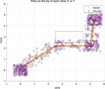
The testing step used was conducted by using the generated waypoints in Table III. Therefore, after using A* to generate the path, the navigation process starts while using the depth/IMU localization. The shown path in Figs. 21–24 shows the different sensors.
Depth camera localization measurements.

Localization measurements from Kobuki odometry solution and IMU pose measurements.

X and Y measurements with respect to time.

Zoomed view on the recorded X and Y measurements.

Localization from the developed sensor fusion approach using CNN.

X and Y measurements with respect to time.

Figures 25–27 show the results from the developed fusion approach as “imu corrected,” with the camera pose measurements to show the enhancement of the frequency at which the algorithm is operating.
Zoomed view on collected X and Y measurements.

Figure 28 shows the error and the error percentage, respectively. Errors were calculated by subtracting the measured localization values for the robot odometry solution from the corrected IMU pose measurements.
The error and error percentages for X and Y values.

4.3. Comparison between CCN and ANN
While setting the hidden layers and hidden neurons values constant, two approaches of neural networks were used: ANN (using MATLAB) and CCN (using ROS-python). The hidden neurons’ values for both approaches were forced to be 10, 15, and 20 in one hidden layer, where the training percentage varies from 60% to 100% with a 10% increment. This step is to show the superiority of CNN over ANN using the same path from Fig. 21.
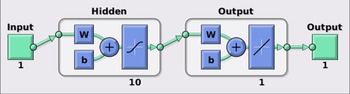
All neural networks shown above had two layers topology, the difference was in the hidden neurons. So, the hidden neurons were 10, 15, and 20 for the first layer, where the second layer is an output layer. Figure 29 shows the topology of an ANN generated network for x axis.
The topology of the ANN generated network used in MATLAB for x axis.

As shown, in the previous Fig. 29, the ANN has 10 neurons in the first layer and one neuron in the second layer, 1-10-1 topology. The neurons are activated through a sigmoid activation function for the input
 $z$
in every neuron as shown in Eq. (24). Each axis was separately implemented and trained by a network.
 \begin{equation}\sigma \!\left(z\right)=\frac{1}{1+e^{-z}}\end{equation}
Comparison of average errors with different network sizes, and training percentages before and after normalization.

The used CCN was modified to keep constructing new layers forcefully until the desired number of layers is achieved, to fairly compare the CCN performance to the ANN. This is achieved by increasing the error to the threshold.
The test was conducted using normalized and non-normalized training pose measurements. While Table V shows the difference between the CCN and ANN, it also shows the advantage of using normalized pose measurements as the errors were lower for different number of hidden layers. It is noteworthy that Table V shows the results for 10, 15, and 20 hidden layers for illustration purposes; however, the algorithm showed the best performance with 12 hidden layers as shown earlier.
In the previous tests, two main conclusions were reached. Eighty percent of the training set was observed to provide the lowest number of errors. Second, CCN was observed to give better performance and lower errors than ANN, while keeping the other parameters constant. This conclusion would verify the advantage of using CCN over ANN.
Details of the constructive CCN for the path in the mechatronics lab.

Details of the best achieved ANN for the path in the mechatronics lab.

Results obtained in the literature using similar methodologies.

Table VI shows the performance achieved after applying the pose measured values from the IMU solutions to the CCN developed approach with 80% training set. As illustrated, the associated errors were low enough to consider this method as a suitable substitute for the depth camera pose solution and depending on the IMU estimated solution. It is not always feasible to depend on the navigation process on the pose measurements from the depth camera, and the IMU pose measurements cannot be considered reliable. The developed approach proves to utilize both sensors to enhance the localization performance for indoor environments, which makes it more accurate and always available. Comparatively, the best performance that was recorded by the ANN is shown in Table VII.
The obtained results were compared to other approaches from literature and observed to be among the lowest errors. Table VIII shows the average errors for selected literature that have used INS or depth camera sensor fusion, along with their fusion method.
5. Conclusion
To enhance the process of navigation of mobile robots, three main tasks were selected, which are mapping, localization, and path planning. The focus of this work was on the localization part. Mapping was performed in advance and was fed to the path-planning algorithm as a cost map. The path-planning algorithm, which is based on A*, was able to reach the destination with the lowest possible cost, resulting in the planned path. To optimize the path, minimizing the waypoints was needed to reach the destination. This is performed by changing the orientation points in the path to be the new waypoints while keeping the distances unchanged.
Localization is another important part of the navigation process. A neural network method, called feedforward cascade correlation, was selected to enhance the localization part of the navigation. The input of the neural network is the calculated pose values from the IMU, and the output is the collected measured pose values from the depth camera solution. The performance of the neural network was compared to the GPS/IMU XSens solution in the outdoor environment and to the Kobuki robot odometry solution in the indoor environment.
Based on the obtained errors, the CCN type of the neural network was proved to be better than ANN type. Moreover, the training set percentage of the network was selected based on the lowest error given, as explained in Section 4. The results showed that the error highly increases when the training data are overfitted (100%) or underfitted (60%). Therefore, having the training set from 70% to 90% was comparatively more stable for the given task than the 100% and 60% training sets. The training set percentage was set to 80%, since it had the lowest associated errors.
Author contributions
The work was developed and implemented by Alkhawaja and supervised by the project advisors.
Financial support
Not funded.
Conflicts of interest
We have no conflicts of interest to disclose.