2 Experimental set-up

The measurements used in this work were carried out in TCABR tokamak. This is a machine with a hydrogen plasma and circular shape with major radius $R_{o}=0.615~\text{m}$ , minor radius $a=0.18~\text{m}$ , toroidal magnetic field $B_{t}=1.1~\text{T}$ , central electron temperature around 0.5 keV, last closed field surface (LFCS) temperature around 15 eV and density around $1\times 10^{18}~\text{m}^{-3}$ . The duration of the discharges in steady state conditions of the main parameters is approximately 100 ms with a plasma current of up to 90 kA. In the experiments presented here the magnetic activity measured by a set of Mirnov coils distributed along the poloidal direction was low. These conditions were used to discard effects of magnetic perturbations due to large magnetic islands, as sometimes occurs in TCABR discharges (Nascimento et al. Reference Nascimento, Kuznetsov, Guimarães-Filho, Chamaa-Neto, Usuriaga, Fonseca, Galvão, Caldas, Severo and Semenov2007; Guimarães-Filho et al. Reference Guimarães-Filho, Caldas, Viana, Heller, Nascimento, Kuznetsov and Bengtson2008).

The experimental data were collected using a five pin probe (LP5p) installed in the equatorial plane of the low field side of TCABR. A radial exploration was performed changing the radial position of the LP5p on a shot-by-shot basis, from 18.5 to 20.0 cm in steps of 0.5 cm. Therefore, the collected data allowed us to explore the behaviour of the turbulence in the SOL, especially the coherent structures. For the LP5p, the five pins were configured in different ways to characterize several aspects of the turbulence, these configurations will be presented in the next sections. The potential signals were measured using a voltage divider with a grounded resistor of $500~\text{k}\unicode[STIX]{x03A9}$ which also assured the isolation for the triple probe technique array. The fluctuating potential $V_{f}$ , positive triple probe potential $V_{+}$ and sweep probe potential $V_{R}$ were measured using a voltage divider. For the saturation current $I_{s}$ and the sweep probe current $I_{R}$ , the measurements were done using a shunt resistor of $10~\unicode[STIX]{x03A9}$ . For all measurements, an operational amplifier was used to couple the impedance of the measurement circuit and the coaxial cable. The data were acquired with an analogue to digital converter at a rate of $2~\text{MS}/\text{s}$ (NI PXIe 6363).

3 Correction in the mean temperature calculation due to the sheath expansion

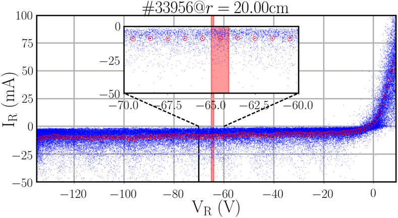
In the introduction a way to consider the sheath expansion effect in the characteristic function of the Langmuir probe was discussed. Therefore, collected data were used to compare the results using the simplified equation (1.1) and the four parameters (1.2) to fit the characteristic voltage–current curve. In order to perform the fit, the data collected during several sweeps with the plasma in almost stationary conditions were grouped according to the applied voltage and the corresponding mean current values were calculated. The original points are shown as small blue dots in figure 1 and the mean values by large red points. Following Theiler et al. (Reference Theiler, Furno, Kuenlin, Marmillod and Fasoli2011) the maximum potential taken into account for the curve fit must fulfil the condition $V_{max}>V_{f}+k_{B}T_{e}$ to avoid the effect of suprathermal electrons. In figure 1 the amplified region shows a light red box indicating the raw points (blue) used to get the mean value point (red). The uncertainty of those mean points is calculated as the standard deviation of the mean ( $\unicode[STIX]{x1D70E}/\sqrt{N}$ ). A nonlinear least squared fit with the Gauss–Marquardt method was used to find the parameters of functions (1.1) and (1.2) considering the above mentioned uncertainties.

Figure 1.

Raw data (blue dots) for the $I_{R}$ as a function of $V_{R}$ and the mean values for the current for a set of potentials (red squares). In the inset, the points in the light red box are those used to get the mean value which is represented by the red circles. The standard deviation of the mean is used as the uncertainty but it is too low to appear as an error bar. These data correspond to discharge $\#33956$ with the probe at $r=20.00~\text{cm}$ .

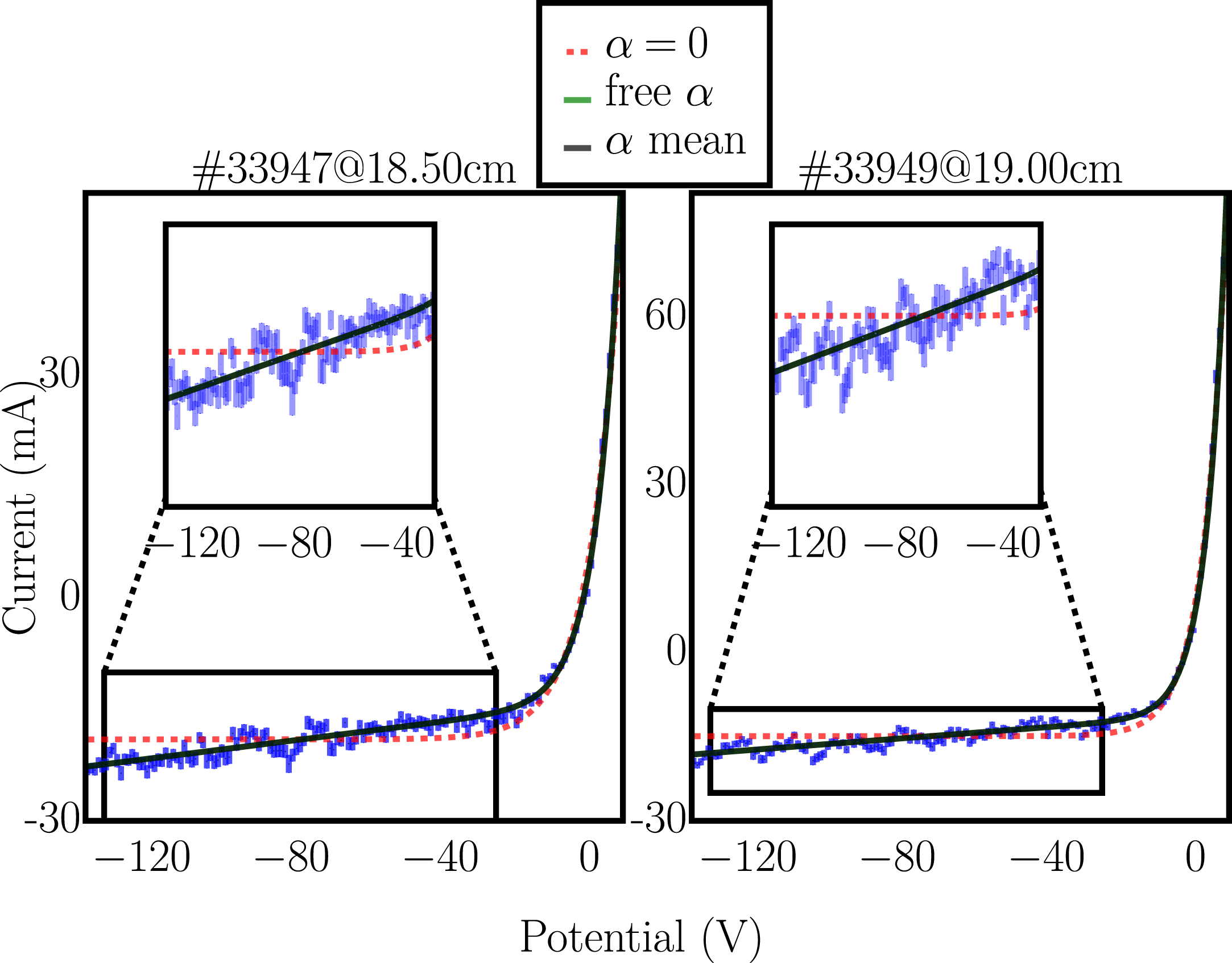
Figure 2 shows examples of the fitting of the characteristic functions applied to the collected data at two different radial positions in the SOL. As can be seen in this figure, equation (1.1) cannot account for the increase in the absolute value of the saturation current at negative potentials. This effect is produced by the expansion of the plasma sheath which is introduced in the characteristic equation (1.2) via the $\unicode[STIX]{x1D6FC}$ parameter. Since the four parameters of (1.2) are very correlated with each other, a fit with few points gives parameters with large uncertainties, mainly due to the $\unicode[STIX]{x1D6FC}$ parameter (Pereira et al. Reference Pereira, Hernandez, Toufen, Guimarães-Filho, Caldas and Gentle2018). For this reason, the fits using the free $\unicode[STIX]{x1D6FC}$ parameter and the fixed $\unicode[STIX]{x1D6FC}$ parameter (using the average value obtained with data from several discharges with the LP5p at different radial positions) were compared. 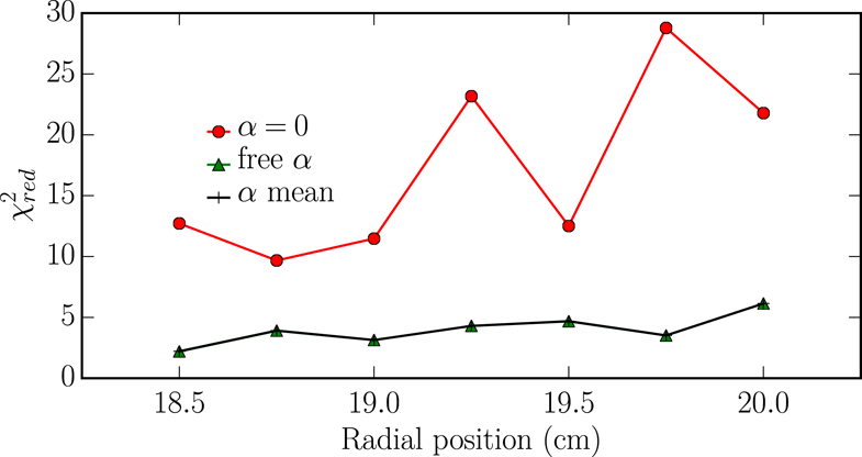The fitted curves obtained by this method are shown in figure 2, where there are two interesting facts: (i) the inclusion of the plasma sheath expansion effect increases the fit accuracy at negative potentials: and (ii) the fit with the parameter $\unicode[STIX]{x1D6FC}$ taken as a free parameter practically overlaps with the fit using a fixed average value. This last point was further explored by calculating the reduced $\unicode[STIX]{x1D712}^{2}$ which indicates the fit quality; a better fit implies a lower $\unicode[STIX]{x1D712}^{2}$ (a reduced $\unicode[STIX]{x1D712}^{2}$ approaches one for fits with a good model and uncertainties). Figure 3 shows the results for several discharges with the LP5p at different radial positions. It can be seen that the inclusion of sheath expansion substantially reduces $\unicode[STIX]{x1D712}^{2}$ , in agreement with the qualitative observations that it increases the quality of the fit. Furthermore, the choice of a fixed mean value for $\unicode[STIX]{x1D6FC}$ furnishes results of the same quality as if $\unicode[STIX]{x1D6FC}$ was obtained from the fit process of just the considered data (the ‘free alpha’ results).

Figure 2.

Examples of fits for the probe characteristic curve given by (1.1) (red). Also, the curve fit including the alpha parameter using (1.2) (green) and assuming a fixed mean value (black). For the last two cases there is an overlap of the curves. The zoom is shown for the negative potential which is the region where the plasma sheath becomes an important effect.

In the standard triple probe technique, the Langmuir model of (1.1) ( $\unicode[STIX]{x1D6FC}=0$ ) is used to obtain the temperature formula given by (1.3). But as was shown above, the inclusion of the expansion sheath is necessary to have an accurate model for the probe response. These results suggest that an enhancement should be performed in the calculation equation for the triple probe technique, a topic that has been discussed in Weinlich & Carlson (Reference Weinlich and Carlson1997), Laux (Reference Laux2001), Theiler et al. (Reference Theiler, Furno, Kuenlin, Marmillod and Fasoli2011), Ghosh et al. (Reference Ghosh, Barada, Chattopadhyay, Ghosh and Bora2015). Therefore, the expression to compute the temperature for the triple probe technique was recalculated using (1.2).

Figure 3.

Reduced $\unicode[STIX]{x1D712}^{2}$ for the three fit methods as a function of the radial position. It is important to note the overlap when the $\unicode[STIX]{x1D6FC}$ parameter is fitted and when its mean value is used.

Figure 4.

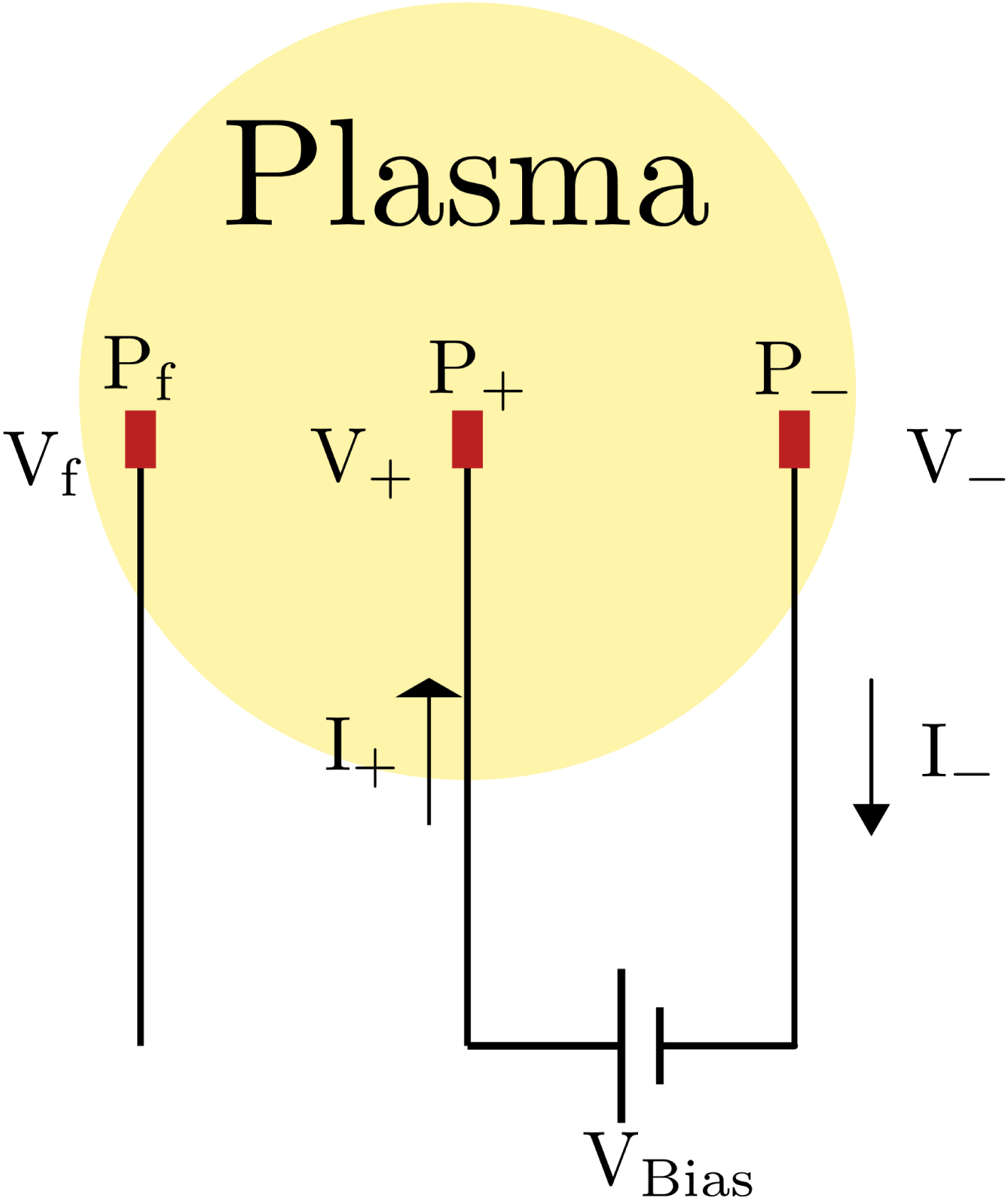
Currents and potentials for the triple probe configuration.

The typical configuration of the triple probe pins is shown in figure 4: two pins are biased with a potential between them and the third pin is floating. The fact that $I_{+}+I_{-}=0$ is used to calculate the temperature for the triple probe, leads to the relation

(3.1) $$\begin{eqnarray}\displaystyle \frac{\displaystyle 1}{\displaystyle 2}=\frac{\displaystyle I_{+}}{\displaystyle I_{+}-I_{-}}. & & \displaystyle\end{eqnarray}$$

Using expression (1.2) for $I_{+}$ and $I_{-}$

(3.2)

where the fact that the potential difference between the $V_{+}$ and $V_{-}$ pins is equal to the applied potential of the source is used

(3.3) $$\begin{eqnarray}\displaystyle V_{Bias}=V_{+}-V_{-} & & \displaystyle\end{eqnarray}$$

as can be seen in figure 4. Also, as $eV_{Bias}$ is several times the temperature in the edge and SOL regions (around 10 eV while $V_{Bias}$ is around 150 V) this implies the cancellation of the term in (3.2). Finally, solving for the temperature, we obtain

(3.4) $$\begin{eqnarray}\displaystyle \frac{\displaystyle kT}{\displaystyle e}=\frac{\displaystyle V_{+}-V_{f}}{\displaystyle \ln (2-\unicode[STIX]{x1D6FC}(2(V_{+}-V_{f})-V_{Bias}))}. & & \displaystyle\end{eqnarray}$$

From the result (3.4), it can be seen that this expression has an additional term that depends on $\unicode[STIX]{x1D6FC}$ . It is important to note that the last expression does not need the measurement of the signal $V_{-}$ , but the value of the bias potential to perform the calculation. A similar expression is proposed in Theiler et al. (Reference Theiler, Furno, Kuenlin, Marmillod and Fasoli2011) using a more involved model that also includes the effect of the stray capacitance of circuits to ground.

Figure 5.

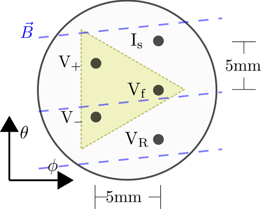
Pin configuration for comparison between triple probe and sweep potential techniques. The shadowed triangle shows the spatial distribution of the triple probe array of pins to measure the floating potential $V_{f}$ and the biased pins $V_{-}$ and $V_{+}$ . The $V_{R}$ pin is where the sweep potential is set and the $I_{s}$ is the pin where the saturation current is measured. The poloidal, $\unicode[STIX]{x1D703}$ , and toroidal, $\unicode[STIX]{x1D719}$ , directions are shown. Also shown is the pin distance and the magnetic field line tilt. Each pin has 4.0 mm length.

In order to test the effect of the correction in the triple probe temperature equation, the triple probe and Langmuir sweep probe techniques were used at the same discharges and radial position. To perform these measurements the five pin probe in the configuration shown in figure 5 was used. 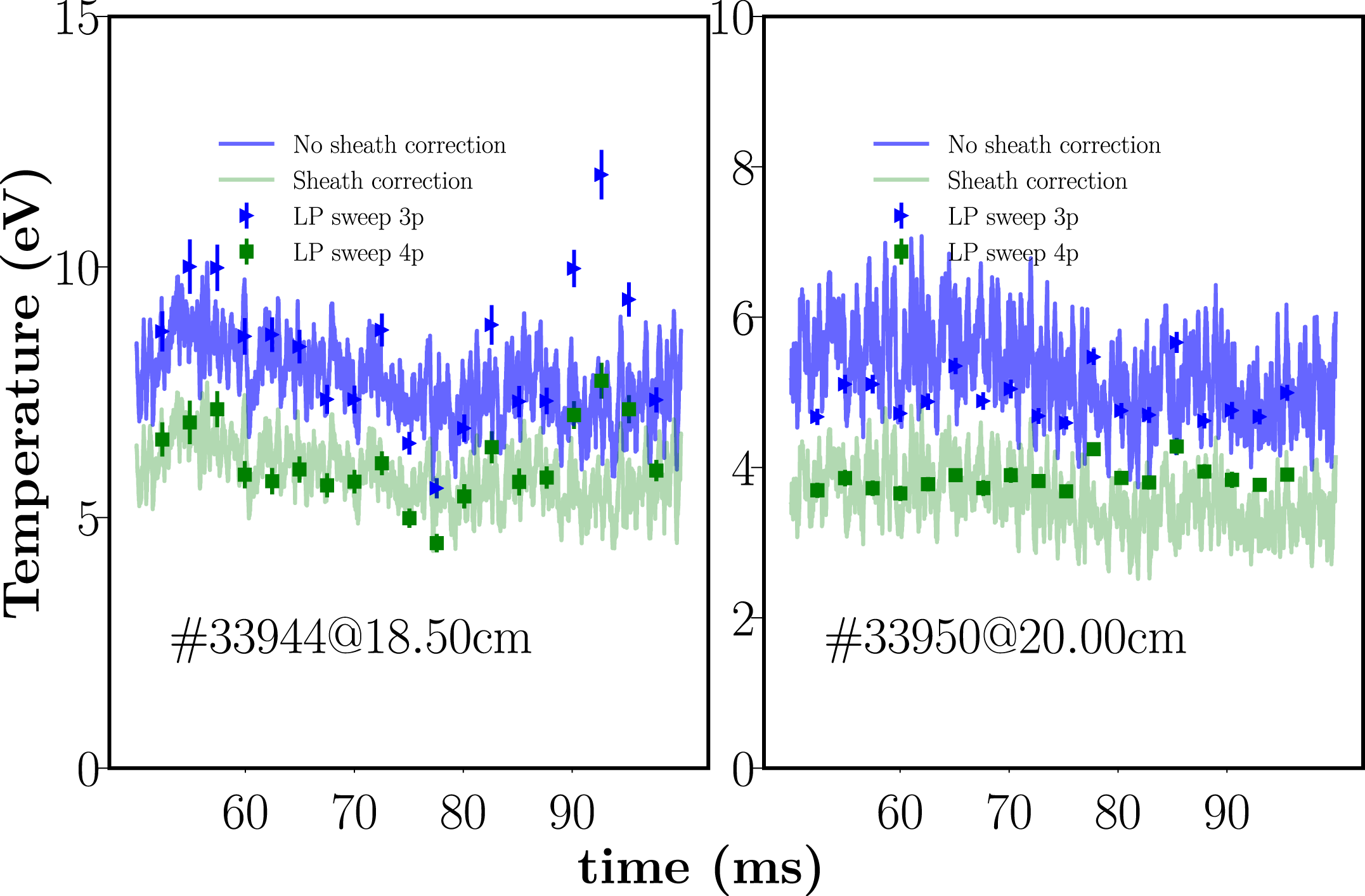For the triple probe, a moving average of ${\sim}500$ points was used ( $250$ points before and $250$ points after), implying a total time of $250~\unicode[STIX]{x03BC}\text{s}$ around each point. In the case of the sweep potential, a sinusoidal signal with a frequency around 1.5 kHz was used. For the calculation at each point four complete cycles were used, that is, four rising ramps and four falling ramps. Moreover, the model with the sheath expansion was used. The measurements were done in a set of discharges where the LP5p was plunged at different radial positions in SOL, ranging from 18.5 to 20.0 cm. As in TCABR the last closed flux surface is at 18.0 cm, in the measurements, the probe was in the SOL region. Figure 6 presents the results for the temperature as a function of time at two different radial positions using the triple probe with and without the correction due to the parameter $\unicode[STIX]{x1D6FC}$ . Also shown is the temperature calculated using just the corrected sweeping probe technique since, as has been shown above, the inclusion of the sheath expansion is necessary to properly fit the characteristic curve. As expected, the measurements with the corrected triple probe agree with those of the corrected sweep probe technique.

Figure 6.

Comparison of the temperature calculated for discharges at radial positions 18.5 (#33944) and 20.0 cm (#33950). The blue signal shows the calculation using the regular triple probe expression, while that in red shows the calculation considering the sheath expansion correction. The green (blue) shows the temperature calculated with the corrected (uncorrected) sweep potential technique.

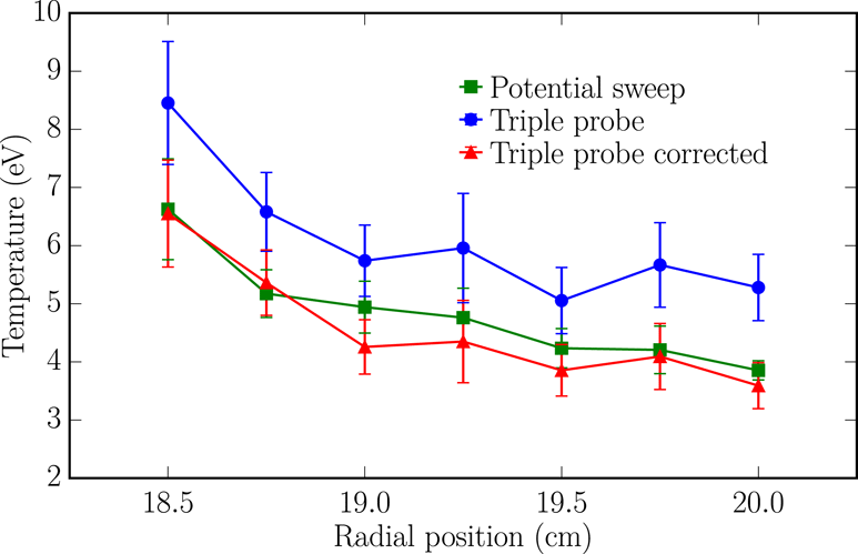
As the LP5p was set at different radial positions, the characteristic profile for the tokamak border was obtained, and the results are shown in figure 7. As is normal in tokamak plasmas, the temperature decreases in the SOL. It is worth noting that the temperature overestimation with the non-corrected triple probe technique can be higher than $50\,\%$ . The overestimation of the temperature value could be a relevant error when the velocity $\boldsymbol{E}_{r}\times \boldsymbol{B}$ is calculated in the poloidal direction, due to the dependence of the plasma potential with temperature.

Figure 7.

The temperature as a function of the radial position for the complete set of discharges obtained by Langmuir sweep and triple probe (with and without the correction due to the $\unicode[STIX]{x1D6FC}$ parameter) techniques.

4 Burst temperature from triple probe and Langmuir sweep probe methods

In this section, the effects of bursts (density peaks associated with coherent structures) on temperature measurements are presented. The bursts in TCABR tokamak have similar properties to those described in other machines (Antar et al. Reference Antar, Counsell, Yu, Labombard and Devynck2003): they appear in the ion saturation current ( $I_{s}$ ) signal as high peaks with exponential decay and a non-Gaussian probability density function (PDF). As usual in bursts studies, burst are classified as the peaks in the $I_{s}$ signal whose maximum values are $2.5\unicode[STIX]{x1D70E}$ above the mean of the time series. Therefore, it is required to normalize the saturation current in terms of the mean value and the standard deviation of the raw data, via

(4.1) $$\begin{eqnarray}\displaystyle I_{s}^{norm}=\frac{\displaystyle I_{s}-\langle I_{s}\rangle }{\displaystyle \unicode[STIX]{x1D70E}_{I_{s}}}, & & \displaystyle\end{eqnarray}$$

where $\langle I_{s}\rangle$ corresponds to the mean value and $\unicode[STIX]{x1D70E}_{I_{s}}$ is the standard deviation.

Figure 8.

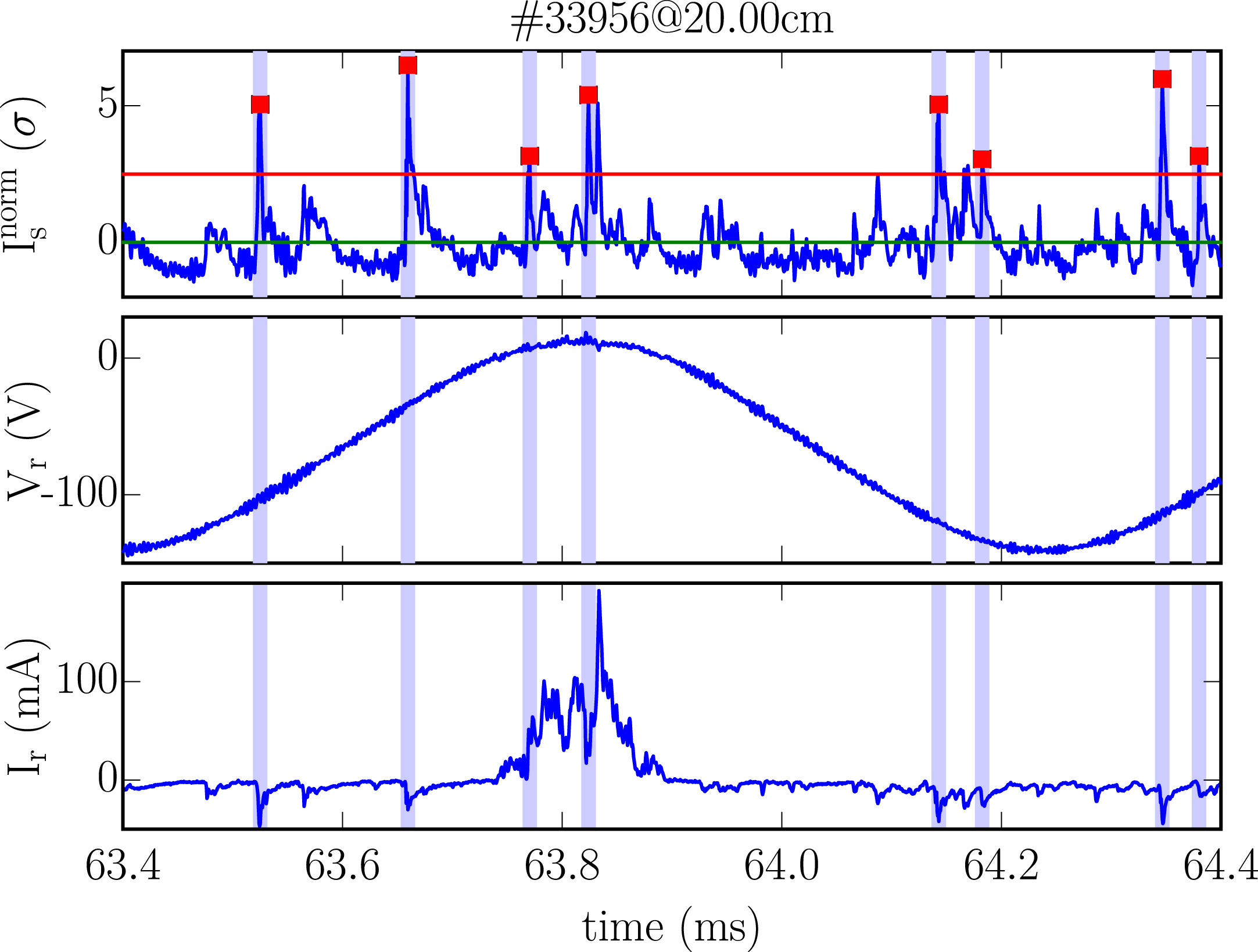
Signals of the normalized saturation current $I_{S}^{norm}$ , sweep potential $V_{r}$ and current $I_{R}$ in a time interval of 1 ms. For $I_{S}^{norm}$ , the burst peaks are marked with red squares. The red line is $\unicode[STIX]{x1D70E}=2.5$ and the light blue boxes are the instant of occurrence of the bursts in other signals. One cycle of the sweep potential is shown.

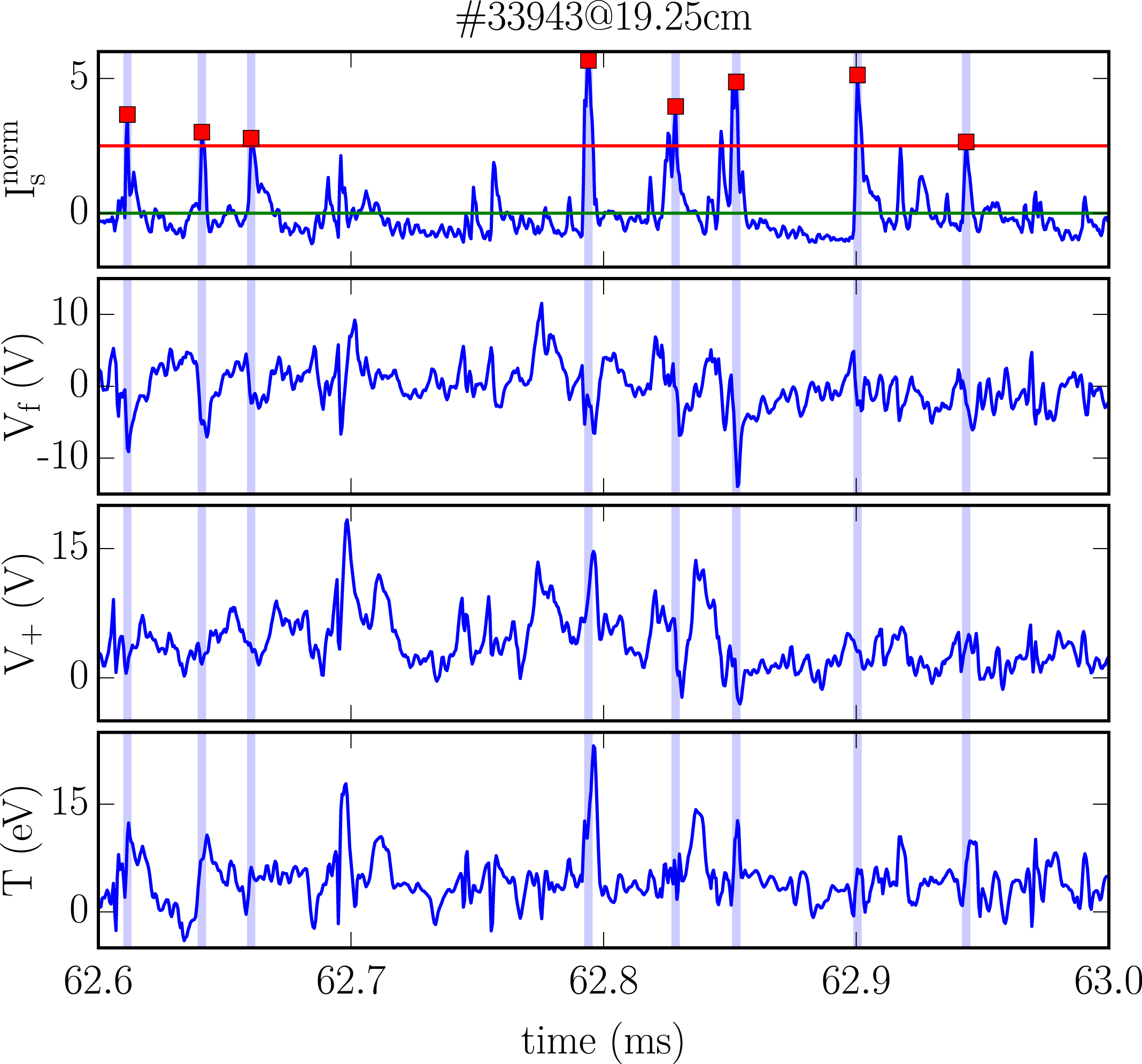
Some examples of those bursts in the saturation current signal are shown in figure 8 where the bursts are identified with red squares.

In the study of bursts, it is common to use the conditional analysis technique (Johnsen, Pecseli & Trulsen Reference Johnsen, Pecseli and Trulsen1986; Antar et al. Reference Antar, Devynck, Garbet and Luckhardt2001a , Reference Antar, Counsell, Yu, Labombard and Devynck2003; Toufen et al. Reference Toufen, Pereira, Guimarães-Filho, Caldas and Gentle2014). This was introduced in the 1980s by Hussain (Reference Hussain1983) with the purpose of retaining coherent components of the signal while averaging out turbulent components of the background. For example, this technique is used to calculate the characteristic size of coherent structures using in the ion saturation current, as shown in Antar et al. (Reference Antar, Counsell, Yu, Labombard and Devynck2003). In the TCABR the characteristic size of coherent structures has been calculated to be approximately 1 cm and increases in the positive radial direction. Also, the conditional analysis serves to calculate the temperature time traces for the coherent structures (Nold et al. Reference Nold, Ribeiro, Ramisch, Huang, Müller, Scott and Stroth2012; Spolaore et al. Reference Spolaore, Vianello, Furno, Carralero, Agostini, Alonso, Avino, Cavazzana, De Masi and Fasoli2015). To perform the temperature measurements, the experimental data were obtained using the LP5p in the configuration shown in figure 5. In this configuration the triple probe and the potential sweep techniques are implemented at the same time for comparison purposes.

Now, we present the results for the conditional analysis applied to the Langmuir sweep technique. In figure 8 we show the signals for the saturation current pin, the Langmuir sweep probe potential $V_{r}$ and current $I_{r}$ . The fast current growth for potentials above zero volts can be seen, and this is a consequence of the exponential behaviour due to the increase in the collection of electrons by the probe. On the contrary, the currents are lower when the potential is negative, as expected by the limited mobility of the ions. Also, during the bursts, the current signal seems to be more negative (negative values become more negative and positive ones tend to zero); this is explained by the fact that the local density value during the bursts is higher than the background one.

To perform the conditional analysis with the Langmuir sweep probe technique, we take the signals of $I_{R}$ and $V_{R}$ , $M_{b}$ points backward and forward the $N_{b}$ bursts maximum to obtain for each signal an array of $N_{b}$ rows and $2M_{b}+1$ columns. In the case of our analysis, $M_{b}$ was chosen to be 40 points; this number of points at the acquisition rate of 2 Msps gives a time $\unicode[STIX]{x0394}t$ of $\pm 20~\unicode[STIX]{x03BC}\text{s}$ . 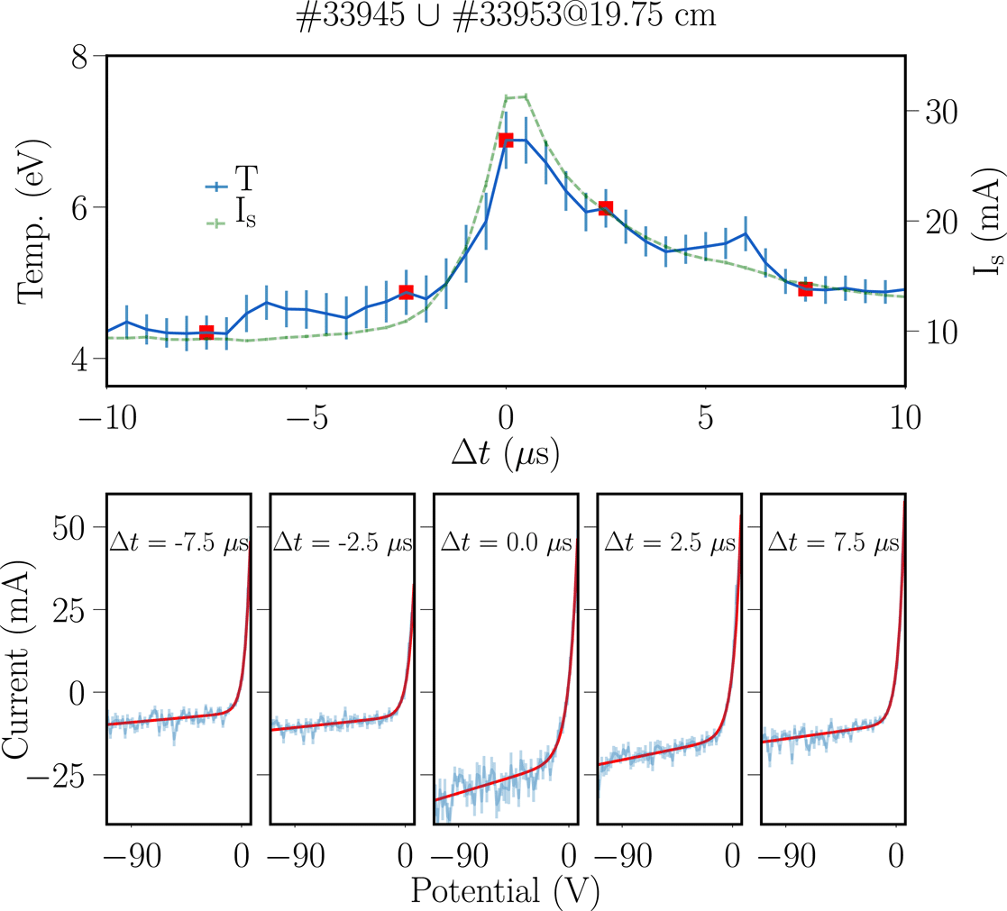Then, we used the $m$ th column of the arrays $I_{R}$ and $V_{R}$ to get a set of $N_{b}$ points. These points were used to fit the probe characteristic function (1.2), giving the temperature, floating potential and saturation current values. Examples of this fit are shown in figure 9, where (a) shows the fitted values of $I_{s}$ and temperature according to the time difference with respect to the maxima burst time (the $I_{s}$ peak detection time). Each point of temperature or saturation current in the figures correspond to the parameters obtained for the fitting of each column of the arrays for $I_{r}$ and $V_{r}$ . Finally, the result of the conditional analysis is a set of three vectors with size $2M_{b}+1$ containing the average time traces for the temperature, saturation current and floating potential. This technique was also used in the works presented in Nold et al. (Reference Nold, Ribeiro, Ramisch, Huang, Müller, Scott and Stroth2012) and Pereira et al. (Reference Pereira, Hernandez, Toufen, Guimarães-Filho, Caldas and Gentle2018).

Figure 9(b) presents the data of $I_{R}$ and $V_{R}$ and the fitted curve for five different times regarding the peak detection in the nearby $I_{s}$ probe. At the moment of the peak ( $\unicode[STIX]{x0394}t=0~\unicode[STIX]{x03BC}\text{s}$ ), when the saturation current increases to its maximum value, it is possible to see the increase in the slope of the fit for negative values of the potential. An important fact is that the uncertainties of the parameters increase due to the reduction in the number of points used to fit the function (1.2), in this case, the number of points is $N_{b}$ : one point for each detected burst. For this reason, the fit method uses the sheath expansion factor (the $\unicode[STIX]{x1D6FC}$ parameter) obtained from the whole time series fit as a fixed value. As was shown in § 3, this procedure reduces the number of fit parameters without any appreciable change in the fit quality.

Figure 9.

Mean temperature and saturation current burst time traces and fitted function for the characteristic curve of the Langmuir probe using the Langmuir sweep probe technique. The probe was located at 19.75 cm, that is 1.75 cm outside the last closed surface (LCS). Panel (a) presents the result of the conditional analysis for the temperature and saturation current. In panel (b) the data and fits that generated the selected points for several time values are presented, in this case at $-7.5~\unicode[STIX]{x03BC}\text{s}$ and $-2.5~\unicode[STIX]{x03BC}\text{s}$ before the burst peak, at the moment of the bust peak ( $0~\unicode[STIX]{x03BC}\text{s}$ ), at $2.5~\unicode[STIX]{x03BC}\text{s}$ and $7.5~\unicode[STIX]{x03BC}\text{s}$ after the burst peak.

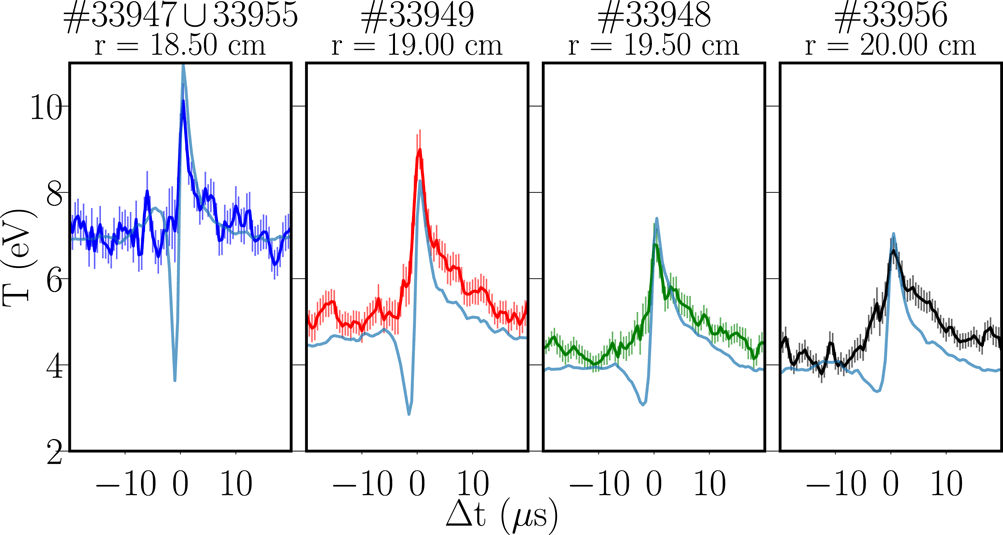
The time traces for the temperature, obtained using the Langmuir sweep probe technique, are shown in figure 10, also the results for the triple probe technique. By comparing the two techniques, it is possible to see that the maximum value of the temperature peak is compatible between them. However, the temperature fall before the peak time, observed with the triple probe, is not present in the Langmuir sweep probe measurements. This distortion in the measurement with the triple probe is an interesting point that will be discussed below.

Figure 10.

The conditional mean for the temperature measured using the Langmuir sweep probe technique, with the light blue line the temperature calculated using the triple probe technique. The conditional mean is presented for different radial positions.

It is noticeable that there exists a pronounced temperature peak when the maximum of the burst intensity happens. Indeed, the burst temperature is above the surrounding plasma as was shown in Pereira et al. (Reference Pereira, Hernandez, Toufen, Guimarães-Filho, Caldas and Gentle2018). This temperature peak decreases as the radial position increases, indicating a possible cooling of the burst as it goes away from the plasma column. It is interesting that the temperature peak is synchronous with the density peak. A similar result was also obtained in the simulations presented in Nielsen et al. (Reference Nielsen, Rasmussen, Madsen, Xu, Naulin, Olsen, Løiten, Hansen, Yan and Tophøj2017) where the conditional analysis was performed in the data obtained using numerical simulations, and it was also presented in the results obtained in Nold & Holzhauer (Reference Nold and Holzhauer2012) where the conditional analysis was applied to experimental data. The existence of this temperature peak indicates a large energy transport caused by the propagation of the coherent structure associated with the burst, from the plasma column to the SOL and even reaching the chamber wall. Although these measurements are not developed in this work, from the theoretical results, the equations for the energy transport depend explicitly on the temperature fluctuations as is shown in Ross (Reference Ross1992).

To perform the conditional analysis on the triple probe technique the bursts detection times in the signal of the ion saturation current are used as reference times for the signals used to calculate the temperature. As an example, shown in figure 11 are the times for eight bursts. Thus, the conditional analysis computes the average behaviour of the temperature at burst detection time.

Figure 11.

Saturation current and triple probe signals for a short time interval of 0.1 ms. For $I_{s}$ , the burst peaks are shown by the red squares. The red line corresponds to the threshold at $I_{s}^{Norm}=2.5$ (2.5 standard deviations above the mean value) and the light blue boxes show the instants of occurrence of the bursts in other signals.

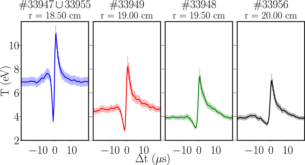
The conditional analysis on the triple probe is calculated in the following way: first, we take the data around the $N_{b}$ detection times for the signals $V_{f}$ and $V_{+}$ , then, the temperature for each of the $N_{b}$ arrays is calculated using the equation that includes the sheath expansion effect (3.4). Finally, with the set of $N_{b}$ temperature conditional signals, the mean value is calculated producing a mean burst temperature time trace. The mean temperature time trace obtained for the bursts using the triple probe conditional average is shown in figure 12. A temperature fall just before the burst peak followed by an abrupt temperature rise exactly at the burst detection time can be seen. The temperature fall is more accentuated for radial positions near the plasma edge (18 cm). However, this behaviour is not presented in the measurement of the Langmuir sweep probe as was shown above. The reason for this difference could be due to the fact that the triple probe measurement depends on the assumption that the plasma is homogeneous in the whole region of the three pins, while, in fact, they are at different spatial positions inside the internal structure of the coherent structure. This kind of burst temperature shape was also obtained in Spolaore et al. (Reference Spolaore, Vianello, Furno, Carralero, Agostini, Alonso, Avino, Cavazzana, De Masi and Fasoli2015).

Figure 12.

Conditional mean for the temperature measured with triple probe technique at different radial positions. The conditional average method was used for this calculation.

Figure 13.

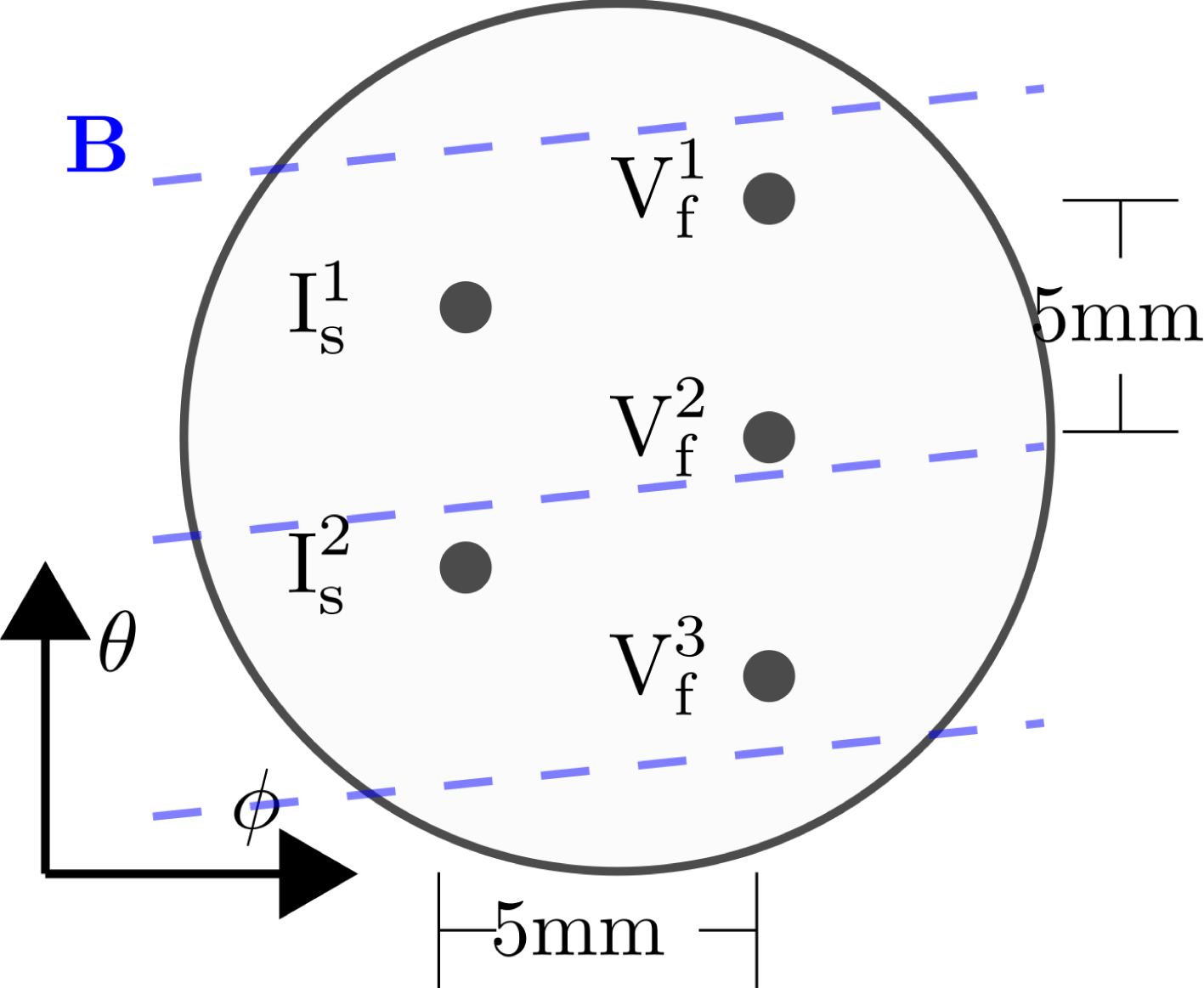
Configuration of the LP5p to analyse the spatial structure of the burst floating potential using conditional analysis.

To study this effect the LP5p was configured as shown in figure 13. Three pins were used to measure the floating potential and the other two pins were used to measure the saturation current, therefore, this configuration allows us to study the spatial structure of the floating potential when bursts are detected in the saturation current pins.

Figure 14.

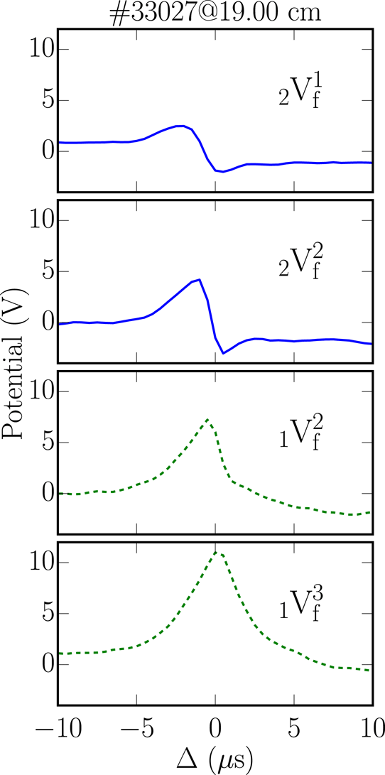
Conditional analysis of the $V_{f}$ signals at different poloidal positions, taking as reference $I_{s}^{1}$ in dashed lines and $I_{s}^{2}$ in continuous lines.

As can be seen in figure 13, if the conditional analysis is applied to signals $V_{f}^{2}$ and $V_{f}^{3}$ and the reference for the burst detection is taken in $I_{s}^{1}$ (i.e. the burst is detected in this pin) we obtain information of the lower side of the structure. On the other hand, if we take $V_{f}^{1}$ and $V_{f}^{2}$ with $I_{s}^{2}$ as the reference, we obtain information of the upper side of the structure. The result of this conditional analysis is shown in figure 14. We can see that the shape of the floating potential depends on the pin position with respect to the reference pin, which is an indication of an internal potential structure inside the coherent structure. The potential structure has a poloidal size ( ${\sim}$ 1 cm), that is of the same order as the LP5p poloidal size, thereby the measurements with triple probe take different parts of the burst internal structure. This fact may compromise the assumption that the three pins are in an almost uniform plasma region, that is one of the main hypotheses used to deduce (1.3) and (3.4). This effect is more pronounced when the distance among the three pins in a perpendicular direction with respect to the magnetic field lines is comparable with the burst characteristic size in that direction. Also, as in Nold & Holzhauer (Reference Nold and Holzhauer2012), that there is no discrepancy between the results of the triple probe technique and the Langmuir probe sweep technique indicates that this problem could be alleviated. For example, the alignment of the probes used in the array with the magnetic field can avoid the inhomogeneity effect.