1 Introduction
There are many regimes of turbulent flow for which the details of turbulence energy spectrum, energy exchanges and mixing are deficient in comparison to those of constant-density turbulent flow (Kolmogorov Reference Kolmogorov1941a
,Reference Kolmogorov
b
; Uberoi Reference Uberoi1963; Helland, VanAtta & Stegen Reference Helland, VanAtta and Stegen1977; Chassaing et al.
Reference Chassaing, Antonia, Anselmet, Joly and Sarkar2002). The current theoretical understanding for results derived directly from the Navier–Stokes equations is substantial in the specialised situation of constant-density turbulent flow in homogeneous (not only isotropic) flow (Orszag Reference Orszag1970; Leslie Reference Leslie1973; McComb Reference McComb1974; Monin & Yaglom Reference Monin and Yaglom1975; Cambon & Scott Reference Cambon and Scott1999). Perturbation renormalisation is one technique for overcoming the statistical closure problem of nonlinear differential equations. The chief advantage of this technique over others is that it does not introduce ad hoc parameters requiring calibration to achieve statistical closure. Through application of renormalisation group theory (RGT) and a few purely mathematical approximations, one can obtain a nonlinear integro-differential equation, whose numerical solution gives a power spectrum and Kolmogorov constant that agree very well with experimental evidence for isotropic turbulence. The first application of this technique to the incompressible Navier–Stokes equations was pioneered by Kraichnan (Reference Kraichnan1959) in a purely Eulerian frame, which he termed the direct-interaction approximation (DIA). Unfortunately Eulerian DIA failed to predict the
 $-5/3$
slope of the turbulence kinetic energy spectrum for the high Reynolds number asymptotic limit. Kraichnan was able to correct this defect using a Lagrangian frame with his Lagrangian DIA (LDIA) (Kraichnan Reference Kraichnan1965), which it is argued separates the sweeping effects of large-scale turbulence from the turbulence cascade energy transfer. Several other methods based upon renormalisation expansions have been developed such as the Wyld diagrams (Wyld Reference Wyld1961), the local energy transfer theory (McComb Reference McComb1974) and the Lagrangian renormalisation approximation (Kaneda Reference Kaneda1981, Reference Kaneda1986) denoted LRA, and refinements of these theories, for example O’Kane & Frederiksen (Reference O’Kane and Frederiksen2004). The sparse direct-interaction perturbation (SDIP) is one of the most recent refinements of LDIA, developed by Kida & Goto (Reference Kida and Goto1997) who noted that sparseness of the nonlinear triadic interactions justified use of the method for turbulence (Goto & Kida Reference Goto and Kida2002). The SDIP method applied to homogeneous isotropic turbulence results in the same equations as LRA (Kida & Goto Reference Kida and Goto1997; Kaneda Reference Kaneda2007). SDIP has also been applied to homogeneous isotropic passive scalar turbulence (Goto & Kida Reference Goto and Kida1999), and turbulent flows with a mean scalar gradient (O’Gorman & Pullin Reference O’Gorman and Pullin2005). Finally, related to DIA is the eddy damped quasi-normal Markovian (EDQNM) theory that shares some aspects with the previous theories but it simplifies two-time correlations by using a phenomenological closure. While EDQNM is not as elegant as LDIA or SDIP, it is still useful because the parameters used in EDQNM can be chosen reasonably well by matching with a few experiments, see Cambon, Jeandel & Mathieu (Reference Cambon, Jeandel and Mathieu1981), Ulitsky & Collins (Reference Ulitsky and Collins2000), Sagaut & Cambon (Reference Sagaut and Cambon2008), Bos & Bertoglio (Reference Bos and Bertoglio2013), and it has been applied to more complex anisotropic flows than LDIA or SDIP. Statistical closure of weakly compressible turbulence in an Eulerian frame has been derived using DIA (Bertoglio, Bataille & Marion Reference Bertoglio, Bataille and Marion2001), which served as a basis for an EDQNM model of this flow.
The present work focuses on zero-Mach variable-density turbulence where the flow is not divergence free. This happens in flows involving a gas with variable temperature and in constant temperature mixing of two fluids of different density. The interest in improving our understanding of turbulence spectra in these flows is twofold. First, from the purely scientific point of view, since it opens the door to other problems with important applications, such as compressible and reactive flow. Second, because a better understanding can lead to better turbulence models, in particular for large-eddy simulation. The zero-Mach number formulation of the Navier–Stokes equations decouples the dynamic and acoustic pressure fields. This facilitates analysis since the energy equation is still not involved in the dynamics, which is a major simplification. But other complications still remain. These include the intimate momentum and mixing coupling (one needs to solve both problems simultaneously) and the nonlinear interactions are less sparse; in the terminology of SDIP, see Goto & Kida (Reference Goto and Kida2002). Consequently, the variable-density triadic wavemode interactions studied here are more complex than those of constant-density flows (Domaradzki & Rogallo Reference Domaradzki and Rogallo1990; Ohkitani & Kida Reference Ohkitani and Kida1992; Waleffe Reference Waleffe1992; Brasseur & Wei Reference Brasseur and Wei1994).
Furthermore, the proper form of the power spectrum, or analogous quantity, that should be used to describe the energy of different wavemodes remains open. For example, Kida & Orszag (Reference Kida and Orszag1990) proposed to consider the power spectrum of  , where
 and
 denote the density and velocity, respectively, in their study of compressible turbulence. While this combination of variables form a true spectral density, it is obscure why this form is the correct mathematical representation of interaction between momentum and density. More recently, Kolla et al. (Reference Kolla, Hawkes, Kerstein, Swaminatham and Chen2014) have considered the symmetrised mixed velocity–momentum two-point spectra, where momentum refers to
 combined. Here, the point of view is to consider the standard quantity that requires closure in variable-density turbulent flow, being the Favre averaged Reynolds stress tensor
 $\tilde{\unicode[STIX]{x1D619}}_{ij}$
(Favre Reference Favre1965a
,Reference Favre
b
), defined by

where overbar and primes denote Reynolds averages and fluctuations, respectively. Explicit Reynolds averages are used on the right-hand side of (1.1) to avoid obfuscating the interactions and have explicitly assumed that the turbulence is isotropic, and in consequence the turbulence flux is not present  . The first term on the right-hand side of (1.1) is the constant-density equivalent (but note that it is not the same as the incompressible Reynolds stress tensor because
 contains density effects hidden in its dynamics). The second term on the right-hand side of (1.1) is the proper triple field interaction, which when studied from the point of view of the Fourier duality, requires us to define the three-point correlation tensor

Evidently,
 $\overline{\unicode[STIX]{x1D70C}^{\prime }u_{i}^{\prime }\boldsymbol{u}_{\boldsymbol{j}}^{\prime }}=\unicode[STIX]{x1D61B}_{ij}(\mathbf{0},\mathbf{0})$
, but more importantly the associated spectral object is

where it can be determined by Fourier inversion, setting  , that

The object
 $\unicode[STIX]{x1D6E9}_{ij}$
is a three-point quantity dependent upon six coordinates, which is of much larger complexity in comparison with the usual two-point quantities associated with standard incompressible turbulence theory. Invoking statistical isotropy does not reduce this object to a double shell spectrum because there is an angular invariant between
 and
 that must be retained explicitly. For these reasons, this paper describes an alternative approach (complementary to that just described) to improve on our understanding of the spectral properties of variable-density turbulence. The present analysis is restricted to isotropic turbulence; even in this simple case such analysis is still both challenging and interesting.
2 Statement of the problem
The governing equations are presented next, followed by some derived equations that will be used throughout the paper. The density
 $\unicode[STIX]{x1D70C}$
is defined by an ideal-gas-based state relationship to a scalar
 (temperature like), expressed in Cartesian coordinates
 , according to

where  has been normalised by the reference density
 and
 $\unicode[STIX]{x1D6FC}$
, a gas expansion-like coefficient, is a constant. It is presumed that
 is always true, which will turn out to be consistent with the asymptotic approach described later. The conservation of mass, employing the Einstein summation convention, is governed by the continuity equation

where
 $u_{\boldsymbol{j}}$
denotes the components of the Eulerian velocity fluctuation vector, which remains dimensional; it is assumed that the mean velocity is zero. The conservation of linear momentum is governed by the Navier–Stokes equations, which can be combined with the continuity equation to describe the evolution of the velocity, according to

where  denotes the modified pressure, divided by
 $\unicode[STIX]{x1D70C}_{0}$
, that also includes the isotropic part of the true linear viscous stress tensor,
 $\unicode[STIX]{x1D708}_{0}=\unicode[STIX]{x1D707}_{0}/\unicode[STIX]{x1D70C}_{0}$
denotes the kinematic viscosity (
 $\unicode[STIX]{x1D707}_{0}$
is interpreted as the dynamic viscosity of the fluid in the same state at which
 $\unicode[STIX]{x1D70C}_{0}$
is evaluated) and
 $f_{l}$
denotes a body force. It is assumed that
 $\unicode[STIX]{x1D708}_{0}$
is a constant, although all transport parameters are functions of the fluid state in variable-density flow; this detail is neglected as these effects are of secondary importance, which will become clear shortly. Fluctuations in scalar
 evolve according to

where  denotes the Schmidt number, which is assumed constant, and
 $g$
a scalar source or forcing function. Taking the partial time derivative of (2.1) and eliminating the partial time derivatives of
 $\hat{\unicode[STIX]{x1D70C}}$
and
 $\unicode[STIX]{x1D719}$
using (2.2) and (2.4) respectively, it can be shown that

In the development of the statistical closure, to be discussed below, the momentum and scalar sources,
 $f_{l}$
and
 $g$
, have spectral content only at large wavelengths and are therefore omitted, under the assumption of turbulence energy flux locality (Zhou Reference Zhou1993; Eyink Reference Eyink2005; Domaradzki & Carati Reference Domaradzki and Carati2007), from the following theoretical development which focuses on the turbulence spectra at high wavenumbers. When comparing to direct numerical simulations, the source terms are retained since they are the driving forces of the turbulent flow. The pressure Poisson equation acting at small scales can be obtained by partially differentiating (2.5) with respect to
 , neglecting
 $f_{l}$
and
 $g$
and making use of (2.3), which after some rearrangement results in

where arguments have been omitted for brevity. The dependence of  upon
 in (2.6) appears through the presence of the inverse density, which multiplies several terms and the explicit presence of
 on the right-hand side of the equation.
3 Theoretical considerations
Several definitions, auxiliary quantities and transformations of the primitive equations are introduced at this point for later use.
3.1 Lagrangian frame of reference
Approximate solutions to the statistical problem of turbulence have been found to successfully predict inertial scaling laws when using a Lagrangian frame (Kraichnan Reference Kraichnan1965; Kaneda Reference Kaneda1986). The transformation from the Eulerian to the Lagrangian frame uses the following map

where  describes the position of a fluid particle at time
 that was measured to be at position
 at time
 . The Lagrangian map evolves according to

and satisfies the initial condition  . The Lagrangian velocity
 $v_{l}$
and scalar
 $\unicode[STIX]{x1D706}$
are related to their corresponding Eulerian fields by the following convolutions

and

It follows that  and
 from the initial condition of the Lagrangian map.
3.2 Statistical quantities
The purpose of this work is to obtain closure of the principal semi-Lagrangian statistical correlations of interest, which for  are defined by


where an overbar denotes ensemble average. The arguments on the left-hand side are a result of statistical homogeneity and stationarity. Note that (3.6) and (3.7) are different statistics when 
The analysis that will be discussed produces spectral quantities valid at high wavenumbers, where the only relevant parameters are viscosity and the corresponding turbulence dissipation rates. The volumetric dissipation rate of the turbulence kinetic energy  is defined by

where the full viscous stress tensor is given by

and  is the Kronecker delta symbol, as opposed to the pseudo-stress tensor used in (2.3) (which is only advantageous computationally), to ensure consistency with the usual transport equation for turbulence kinetic energy. Similarly, the volumetric dissipation rate of turbulence scalar fluctuations
 is defined as

Finally, the volumetric enstrophy is defined as

These statistics are not dependent on  or
 due to statistical homogeneity and stationarity. The specific (per unit mass Favre averaged) turbulence,
 $\tilde{\unicode[STIX]{x1D700}}$
, and scalar,
 $\tilde{\unicode[STIX]{x1D712}}$
, dissipation rates are related to the volumetric forms by
 and
 , respectively, where
 denotes the ensemble average of
 . Owing to the state relationship and the normalisation used here,
 , but the explicit symbol
 $\bar{\unicode[STIX]{x1D70C}}$
is retained to ensure
 and
 are not confused with
 and
 .
3.3 Spectral representation
Derivation of the necessary spectra requires performing a transform of the governing equations to Fourier space. This confines the fluid motion into a periodic cube defined by the characteristic length
 $L$
. Consider the Fourier series expansion of the primitive quantities


where the summations are taken over the integer triplets,  , that define the wavevector
 . The Fourier coefficients are given by the standard formulas


where the integrals are performed over a periodic cubic domain.
Introducing the Fourier series expansions of the primitive quantities into the governing equations, multiplying by the complex conjugate of the basis function and integrating over the periodic cubic domain results in the following evolution equation for the Eulerian velocity spectral coefficients

Similarly, the Fourier coefficients of
 $\unicode[STIX]{x1D719}$
evolve according to

The mass constraint, equation (2.5), becomes

The Fourier coefficients of the Lagrangian map obey

with the initial condition

The Lagrangian velocity can be determined from the convolution sum, see (3.3), giving

while its evolution equation is described by

Similarly, the Lagrangian scalar can be determined using the convolution sum, equation (3.4), giving

and the corresponding evolution equation

3.4 Relation of statistical quantities to spectral description
Of particular interest are the four correlations between Lagrangian and Eulerian spectral primitive quantities. The first is the semi-Lagrangian velocity correlation, where  , defined as

where  . In addition, the semi-Lagrangian scalar-velocity correlations of the first and second kinds, where
 , are defined as

and

where  . Finally, the semi-Lagrangian scalar correlation, where
 , is defined as

respectively, where  . The mass constraint gives the following relationships:


The volumetric turbulence energy dissipation rate can be expressed in terms of the aforementioned semi-Lagrangian spectral correlations

as well as the volumetric turbulence scalar dissipation rate

and the volumetric enstrophy

Note that from (3.36) one can already see that explicit dilatational effects are quadratic in
 $\unicode[STIX]{x1D6FC}$
and therefore any modification of the energy exchanges owing to variable-density effects are, to leading order in
 $\unicode[STIX]{x1D6FC}$
, embedded in
 and not due to
 . Reviewing (3.38) it is also observed that the volumetric turbulence energy dissipation rate is equivalent to twice the product of the volumetric enstrophy and the kinematic viscosity, to leading order in
 $\unicode[STIX]{x1D6FC}$
.
4 Solution procedure
The variable-density turbulence statistical closure problem has two key challenges. First, that the pressure Poisson equation (2.6) does not admit an explicit solution for arbitrary
 $\unicode[STIX]{x1D6FC}$
. Second, that interactions between the primitive fields of velocity and scalar generate further correlations that need to be determined. An asymptotic expansion in the parameter
 $\unicode[STIX]{x1D6FC}$
, henceforth assumed small, is used to make the problem tractable. This approach will produce the well-known constant-density problem to
 $O(1)$
, see Kida & Goto (Reference Kida and Goto1997) and Goto & Kida (Reference Goto and Kida1999), and a new problem to
 $O(\unicode[STIX]{x1D6FC})$
that will contain the main effects of variable density. The sparse direct-interaction closure is then applied to the resulting equations.
4.1 Asymptotic expansion
An asymptotic expansion about the constant-density limit,
 $\unicode[STIX]{x1D6FC}=0$
, is introduced such that

The statistical quantities of interest and the turbulence dissipation rates expand accordingly; superscript in parenthesis always denoting the order in the expansion. The
 $O(1)$
terms of the expansion, superscript
 $(0)$
, correspond to the constant-density solution, which is detailed in appendix A and has been known for some time. What follows is the formulation of the first-order problem,
 $O(\unicode[STIX]{x1D6FC})$
. First, a Helmholtz decomposition of the
 $O(\unicode[STIX]{x1D6FC})$
Eulerian velocity is introduced:

where superscripts ‘s’ and ‘p’ denote the solenoidal and potential splitting, respectively, given by

The projection operators are given by the well-known expressions

The potential Eulerian velocity can be identified from the mass constraint, equation (3.23), by applying the projection definitions, resulting in

This demonstrates the utility of the Helmholtz decomposition, where any source of potential velocity, and consequently dilatation, can be isolated to a pure effect of the
 $O(1)$
scalar field. Expanding (3.21), gathering the
 $O(\unicode[STIX]{x1D6FC})$
terms and introducing the Helmholtz Eulerian velocity decomposition shows that the solenoidal component evolves according to

The asymptotic expansion ensures that the higher-order solenoidal velocity field evolves linearly, although this linearity remains entangled within triadic Fourier sums with fields at the lower order in the expansion, as expected.
The
 $O(\unicode[STIX]{x1D6FC})$
modified pressure can be solved now explicitly by expanding (2.6), introducing Fourier series and using the definitions of the
 $O(1)$
fields, giving

while the
 $O(\unicode[STIX]{x1D6FC})$
Eulerian scalar evolves according to

Similarly, the
 $O(\unicode[STIX]{x1D6FC})$
Lagrangian map evolves according to

whilst satisfying the initial condition  . One can derive the
 $O(\unicode[STIX]{x1D6FC})$
Lagrangian scalar evolution equation using
 , given by

The following decomposition of the
 $O(\unicode[STIX]{x1D6FC})$
Lagrangian velocity is introduced

where  is defined by

which is advantageous since this quantity respects solenoidality instantaneously; i.e.  . Note that
 , equation (4.11), contains both a solenoidal and potential component even under the condition
 . The evolution of
 is governed by

In constructing the complete
 $O(\unicode[STIX]{x1D6FC})$
statistical quantities, it is convenient to first define correlations that become instantaneously (when
 ) solenoidal. The
 $O(\unicode[STIX]{x1D6FC})$
semi-Lagrangian velocity correlations, where
 , are defined as

and

From these definitions it is evident that  . The solenoidal property of both
 and
 ensures that
 and
 respectively. The
 $O(\unicode[STIX]{x1D6FC})$
semi-Lagrangian velocity-scalar correlations of the first kind, where
 , are defined as

and

The solenoidal property of both
 $\tilde{u} _{j}^{(0)}$
and
 ensures that
 and
 respectively. The
 $O(\unicode[STIX]{x1D6FC})$
semi-Lagrangian velocity-scalar correlations of the second kind, where
 , are defined as

and

The
 $O(\unicode[STIX]{x1D6FC})$
semi-Lagrangian scalar correlations, where
 , are defined as

and

From these definitions one has  . The complete
 $O(\unicode[STIX]{x1D6FC})$
semi-Lagrangian statistical quantities, where
 , can now be expressed in terms of the previous statistical correlations, whereby


and

Finally, introducing the asymptotic expansion in (3.9) and (3.11) gives the
 $O(1)$
dissipation rates, defined by

and

as well as the
 $O(\unicode[STIX]{x1D6FC})$
specific turbulence energy and scalar dissipation rates

and

The problem is now completely specified, except for the need to introduce the statistical closure, which is described next.
4.2 Sparse direct-interaction perturbation
The problem of statistical closure is now addressed by employing the sparse direct-interaction perturbation methodology (Kida & Goto Reference Kida and Goto1997) with some modification described below. This technique is comprised of several steps, the first of which involves decomposing the primitive quantities into direct- and non-direct-interaction components. It is then asserted that the non-direct-interaction components possess particular statistical characteristics, which are described by a finite number of non-zero statistical cumulants. The direct-interaction components are subsequently described by an evolution equation linearised about the non-direct-interaction component, a consequence of the perturbation assumption. Closure is then obtained through renormalisation, rather than solving for the non-direct-interaction quantities. For example, the SDIP decomposition of the
 $O(1)$
Eulerian velocity is given by

where  denotes a field where the interaction with the modes
 has been excluded (non-direct-interaction field), while
 denotes the field involving these modes (direct-interaction field). It is required that the wavemodes form a triangle, i.e.
 . The precise wavemodes that are excluded need not be specified at this point. The introduction of
 and
 is a notation simplification with respect to that used in Kida & Goto (Reference Kida and Goto1997) to aid in the transcription of the expressions. Now, the
 $O(1)$
non-direct-interaction Eulerian velocity evolves according to

where the triangle in the summation symbol refers to the sum excluding the wavemodes  ,
 ,
 and the remainder denoted with primes satisfies

No attempt to solve (4.31) is made, and the initial state of the non-direct-interaction Eulerian velocity becomes inconsequential under the condition of statistical stationarity. Presenting this equation however, provides some justification for asserting that only the second-order statistical cumulant (the associated Maclaurin series coefficient of the natural logarithm of the moment-generating function) of the non-direct-interaction Eulerian velocity is non-zero. The statistical influence of the complete convolution sum is assumed to be small by appealing to the central limit theory and accepting that the sum involves a complex hierarchy of interactions. Any bias introduced by partitioning the sum is also assumed to be small as statistical homogeneity makes  sparse and
 almost complete.
The
 $O(1)$
direct interaction Eulerian velocity evolves according to

where the last source term in (4.33) is defined as

and satisfies the initial condition

In order to express the direct-interaction Eulerian velocity field in terms of the non-direct-interaction field, the following response function is defined:

which evolves according to

and satisfies the initial condition  . The projection operator arises from the condition of statistical isotropy, and that the initial condition is non-random. Two key observations are made: that the response is not explicitly dependent on any white noise influencing the system, and that the Eulerian velocity–velocity response is essentially the Green’s function of the
 $O(1)$
direct-interaction Eulerian velocity under the perturbation assumption. Performing the SDIP decomposition of the
 $O(1)$
Eulerian velocity–velocity response, one obtains

such that the
 $O(1)$
non-direct-interaction Eulerian velocity–velocity response evolves according to

whilst satisfying the initial condition

The
 $O(1)$
direct-interaction Eulerian velocity–velocity response evolves according to

where the source term is defined as

and satisfies the initial condition

Note that in the absence of the partial convolution sum, the
 $O(1)$
non-direct-interaction Eulerian velocity–velocity response becomes a non-random process. Based upon this observation, it is asserted that the non-direct-interaction Eulerian velocity–velocity response is statistically independent of all other quantities. Applying Duhamel’s principle gives

By ignoring the functional dependence of the
 $O(1)$
Eulerian velocity–velocity response upon the
 $O(1)$
direct-interaction Eulerian velocity, as it is assumed in SDIP, recursive dependencies on higher-order variational quantities can be avoided in (4.41), such that

An analogous set of equations are developed for  ,
 and
 . Closure of this system of equations is achieved through renormalisation, by ensemble averaging (denoted by an overbar) and discarding
 , gives

where  is the ensemble
 $O(1)$
Lagrangian–Eulerian velocity–velocity response defined as

which respects statistical homogeneity and stationarity. Analogous renormalisation approximations are made for statistical quantities involving  ,
 and
 . Statistical closure of the Lagrangian map is treated in a different manner according to SDIP; performing the decomposition of the
 $O(1)$
Lagrangian map gives

where the
 $O(1)$
non-direct-interaction Lagrangian map evolves according to

and satisfies the initial condition

In this situation, solving for the statistical ensemble of the non-direct-interaction Lagrangian map is preferred over renormalisation, such that

According to Kraichnan (Reference Kraichnan1965), this approach prevents the convective forces of the large scales from entering into the calculation of the inertial energy transfer. Then, the
 $O(1)$
direct-interaction Lagrangian map evolves according to

where the source term is defined as

and satisfies the initial condition

The direct interactions of the Eulerian velocity with the Lagrangian map are neglected in (4.52) to avoid recursive dependencies on higher-order quantities. From Duhamel’s principle one recovers

where the non-direct-interaction Lagrangian map acts as the Green’s function of the direct-interaction Lagrangian map.
4.3 Departure from SDIP for Lagrangian scalars
The
 $O(1)$
statistical correlations and ensemble response quantities involving
 are equivalent to those derived in Kida & Goto (Reference Kida and Goto1997), the results of which have been re-stated in appendix B for completeness. The SDIP theory predicts that the potential component of the
 $O(1)$
semi-Lagrangian Eulerian velocity correlation as well as the
 $O(1)$
semi-Lagrangian scalar-velocity correlation of the first kind are zero only under the restriction of isotropic turbulence. For the
 $O(1)$
scalar statistics, a proposed modification to the standard SDIP theory is now presented. The current SDIP theory is known to estimate the Obukhov–Corrsin constant to be approximately 50 % less than the experimentally observed value (Goto & Kida Reference Goto and Kida1999). This inconsistency was first reported by Kraichnan (Reference Kraichnan1968) using Lagrangian history direct interaction. There is some scatter in the experimental values (Sreenivasan Reference Sreenivasan1996) but the discrepancy with SDIP theory seems too large to be reconcilable. To develop an alternative approximation, first review the definition of the
 $O(1)$
Lagrangian scalar

where it follows from (4.50) that  . The partial derivative of (4.56) with respect to
 evaluated at
 , again using (4.50), is found to be

It follows that the second-order partial derivative of (4.56) with respect to  evaluated at
 is

and the third-order partial derivative of (4.56) with respect to  evaluated at
 is

These equations expose exactly an explicit dependence of the
 $O(1)$
Lagrangian scalar upon the
 $O(1)$
Eulerian velocity. Next, consider the definition of the
 $O(1)$
Lagrangian scalar–scalar response, given by

which satisfies the condition  . Differentiating (4.60) with respect to
 , dividing by
 and then performing a Taylor series about
 results in

The following commutative property of the response

when applied to (4.57)–(4.59) gives


and

No statistical closure assumptions were required to obtain (4.63)–(4.65). To complete the approximation of the
 $O(1)$
Lagrangian scalar–scalar response, substitute (4.63)–(4.65) into (4.61) to arrive at

This method differs from the use of Taylor series by Gotoh, Nagaki & Kaneda (Reference Gotoh, Nagaki and Kaneda2000) to determine representatives that are best approximated by renormalisation. Quantities defined in terms of  can be formulated in an analogous manner to replace the standard SDIP form. Further discussion regarding the order at which the series is truncated,
 , is provided in § 5.
The following derivation of the
 $O(\unicode[STIX]{x1D6FC})$
statistical correlations and ensemble response quantities provide a closed set of equations for the leading variable-density turbulence effects. For brevity, the derivation below has omitted quantities, such as the ensemble
 $O(\unicode[STIX]{x1D6FC})$
Lagrangian velocity response to the
 $O(1)$
Eulerian scalar and the auxiliary Lagrangian velocity–Eulerian scalar correlation, because they were found to be trivial. Application of the SDIP methodology resulted in these quantities being governed by homogeneous differential equations with initial conditions that are satisfied by trivial solutions. It was not assumed a priori that these quantities were irrelevant. The reader interested in the final result of the analysis can skip the following subsections and jump directly to § 5 where the high Reynolds number limit is detailed.
4.3.1 Semi-Lagrangian velocity correlations
In order to obtain statistical closure, the equations governing both the instantaneous and two-time semi-Lagrangian velocity correlations must be established. The
 $O(\unicode[STIX]{x1D6FC})$
instantaneous semi-Lagrangian velocity correlation evolves according to

where the statistical quantities on the right-hand side are stationary and the resultant ensemble averages will not depend on  . The two-time semi-Lagrangian velocity correlation of the first kind evolves according to

and the second kind evolves according to

Applying the SDIP methodology results in the following expressions: for the instantaneous velocity correlation

for the first two-time velocity correlation

and for the second two-time velocity correlation

4.3.2 Lagrangian velocity–velocity responses
It has been determined that two Lagrangian velocity–velocity response quantities are needed to complete the statistical closure of the
 $O(\unicode[STIX]{x1D6FC})$
semi-Lagrangian velocity correlations
 and
 . The ensemble Lagrangian–Eulerian velocity–velocity response of the first kind is defined as

which evolves according to

and satisfies the initial condition  . The first-kind pressure response function to the
 $O(\unicode[STIX]{x1D6FC})$
solenoidal Eulerian velocity is given by

The ensemble Lagrangian–Eulerian velocity–velocity response of the second kind is defined as

which evolves according to

and satisfies the initial condition  . The constant-density pressure response term is defined in appendix B, and the second-kind
 $O(\unicode[STIX]{x1D6FC})$
pressure response function to the
 $O(1)$
Eulerian velocity is given by

Applying the SDIP methodology to (4.74) results in

and for (4.77) gives

4.3.3 Semi-Lagrangian scalar correlations
The instantaneous and two-time semi-Lagrangian scalar correlations evolve according to

The
 $O(\unicode[STIX]{x1D6FC})$
semi-Lagrangian scalar correlation of the first kind, where
 , evolves according to

and the
 $O(\unicode[STIX]{x1D6FC})$
semi-Lagrangian scalar correlation of the second kind, where
 , evolves according to

Applying the SDIP methodology to achieve statistical closure of the instantaneous scalar correlation produces

Application of the SDIP methodology to the third- and fourth-order statistical correlations that appear in (4.82) and (4.83) will retain only the influence of diffusion effects. For (4.82) and (4.83), the proposed alternative approximation by application of a Taylor series to the Lagrangian scalar is applied, see § 4.3, which results in

and

respectively. These new equations will replace the standard SDIP closures and result in improved predictions of the Obukhov–Corrsin constant. The equivalent approximation for the constant-density mixing problem is shown in appendix B.
4.3.4 Lagrangian–Eulerian scalar–scalar response
Completing the statistical closure of the
 $O(\unicode[STIX]{x1D6FC})$
semi-Lagrangian scalar correlations requires one final quantity, the ensemble Lagrangian–Eulerian scalar–scalar response

which evolves according to

and satisfies the initial condition  . Analogous to the earlier treatment of the two-time scalar correlations, the proposed alternative approximation of the
 $O(\unicode[STIX]{x1D6FC})$
Lagrangian scalar results in

4.4 Statistical isotropy
The present analysis is now restricted to statistical isotropy. The wavenumber dependence is made continuous by taking
 $L\rightarrow \infty$
, thus transforming the triadic convolution summations into integrals (Leslie Reference Leslie1973), according to

The tensorial statistical quantities can now be defined in terms of tensorial operators, that respect the mass constraint, and scalar functions, as defined by

Note that  ,
 , and
 . Applying these statistical restrictions to (4.70) results in

where the spectral kernel functions are defined, see Leslie (Reference Leslie1973), as


Similarly the first
 $O(\unicode[STIX]{x1D6FC})$
two-time velocity correlation, equation (4.71), gives

and the second
 $O(\unicode[STIX]{x1D6FC})$
two-time velocity correlation, equation (4.72), gives

with the spectral kernel function defined by

The function  as
 or
 is evaluated by using a series expansion near the limit
 and using the identity
 .
Applying statistical isotropy and stationarity to the first
 $O(\unicode[STIX]{x1D6FC})$
ensemble Lagrangian velocity–velocity response, equation (4.79), gives

whilst satisfying the initial condition  . This initial value problem is equivalent to that of the
 $O(1)$
velocity–velocity response, equation (B 21), hence
 . For the second
 $O(\unicode[STIX]{x1D6FC})$
ensemble Lagrangian velocity–velocity response, equation (4.80), the conditions of statistical isotropy and stationarity give

whilst satisfying the initial condition  . Direct integration of (4.95) and (4.96) with respect to
 , using (B 21) and (4.99), gives respectively

and

These fluctuation–dissipation relationships are a consequence of the dominance of Lagrangian map direct interactions that result in homogeneous linear evolution equations, which resemble LRA.
Statistical stationarity and isotropy applied to (4.84) gives

Similarly for the first
 $O(\unicode[STIX]{x1D6FC})$
two-time scalar correlation, equation (4.85), one has

and the second
 $O(\unicode[STIX]{x1D6FC})$
two-time scalar correlation, equation (4.86), one has

Direct integration of (4.103) and (4.104) with respect to  leads to

Applying the conditions of statistical isotropy and stationarity to the
 $O(\unicode[STIX]{x1D6FC})$
ensemble Lagrangian scalar–scalar response, equation (4.89), gives

which satisfies the initial condition  . This initial value problem is equivalent to that of the
 $O(1)$
scalar–scalar response, equation (B 26), hence
 . Finally, applying the statistical restrictions to the
 $O(1)$
and
 $O(\unicode[STIX]{x1D6FC})$
specific turbulence kinetic and scalar-variance dissipation rates defined by (4.28) and (4.29), produces respectively


5 High Reynolds number limit
Here, the large Reynolds number limit is considered by rescaling the equations in viscous (Kolmogorov) units. For completeness, the previously derived
 $O(1)$
statistical quantities are now stated. Let the Kolmogorov scale be defined by

then the non-dimensional wavenumber and scaled time are

respectively, where  (the Kolmogorov constant) is to be determined below. From dimensional analysis, the
 $O(1)$
instantaneous semi-Lagrangian velocity correlation is of the following similarity form

and the corresponding self-similar response is defined by  . Note that double dagger subscript is employed to distinguish dimensional from non-dimensional quantities, as in Kida & Goto (Reference Kida and Goto1997). Introducing the viscous scaling into (B 19) results in the
 $O(1)$
self-similar instantaneous semi-Lagrangian velocity correlation equation

The inertial transfer of
 $O(1)$
turbulence energy from the production to the dissipation scales is enforced by
 , and the energy dissipation condition, (4.107a
), leads to the relationship that determines
 , given by

Similarly from (B 21), the
 $O(1)$
self-similar Lagrangian velocity–velocity response evolves according to

with initial conditions

From dimensional analysis, the
 $O(\unicode[STIX]{x1D6FC})$
instantaneous semi-Lagrangian velocity correlation adopts the following similarity form:

and the corresponding response function is

Introducing the viscous scaling into (4.92) results in

while the analogous argument concerning the production of turbulence energy from the large scales results, to
 $O(\unicode[STIX]{x1D6FC})$
, in the condition
 ;
 is obtained from the
 $O(\unicode[STIX]{x1D6FC})$
turbulence energy dissipation, (4.107b
), given by

From (4.99), the
 $O(\unicode[STIX]{x1D6FC})$
self-similar Lagrangian–Eulerian velocity–velocity response satisfies

with initial conditions

Finally, the variable-density compensated turbulence energy spectrum can be expressed using the newly introduced functions as

where the ratio of turbulence energy dissipation rates,  , appears explicitly and it accounts for the different dissipation mechanisms that are present in the variable-density flow, up to
 $O(\unicode[STIX]{x1D6FC})$
. The numerical values of the dissipation rates are determined by the production of turbulence occurring at the large scales of the flow and are input parameters in the asymptotic large Reynolds number inertial and dissipation subranges described here. The present theory cannot, as it happens in constant-density flow, give an explanation as to the nature of the large-scale dynamics that generates this energy transfer. The turbulence kinetic energy dissipation and enstrophy spectra are respectively found from

Next, the scalar statistics are considered. From dimensional analysis, the
 $O(1)$
instantaneous semi-Lagrangian scalar correlation has the following similarity form

and the corresponding self-similar response function is defined by  . Introducing the viscous scaling in (B 24), the
 $O(1)$
self-similar instantaneous semi-Lagrangian scalar correlation satisfies

where the inertial transfer of
 $O(1)$
turbulence scalar variance from the production scales is enforced by
 , and the turbulence scalar variance dissipation, (4.108a
), results in a relationship that determines the Obukhov–Corrsin constant
 , given by

Introducing the viscous scaling in (B 27), the
 $O(1)$
self-similar Lagrangian scalar–scalar response has been found analytically to be

Inspection of (5.19) provides some justification for truncating the Taylor series approximation of the
 $O(1)$
Lagrangian scalar–scalar response, equation (4.61), from which this result is based. The first term inside the exponent of the right-hand side of (5.19) accounts for the viscous effects on the response; the second term is a result of the modified approximation, which due to the presence of
 is dependent upon the turbulence kinetic energy spectrum. It is evident that the first term tends to
 $0$
as
 for all
 . The inclusion of the second term results in decay of the response along
 . The shape of the response over the remainder of the
 domain is largely unmodified by the second term. It is anticipated that higher-order terms are not as significant since the sum of these first two terms are non-zero for all
 .
The
 $O(\unicode[STIX]{x1D6FC})$
instantaneous semi-Lagrangian scalar correlation is obtained from (4.102) by observing that the general solution of this equation can be decomposed as the linear superposition of a homogeneous term proportional to
 and a new particular term that needs to be determined. From dimensional grounds, the following similarity form arises:

Introducing the viscous scaling in (4.102), the new
 $O(\unicode[STIX]{x1D6FC})$
self-similar instantaneous semi-Lagrangian scalar correlation satisfies

where the transfer of
 $O(\unicode[STIX]{x1D6FC})$
turbulence scalar variance from the production to inertial scales is enforced by
 ;
 is determined from the
 $O(\unicode[STIX]{x1D6FC})$
turbulence scalar-variance dissipation, (4.108b
), giving

To conclude, one can put together all the terms of the variable-density compensated turbulence scalar-variance spectrum to obtain

where

with  is the leading-order variable-density mixing-to-turbulence flux intensity ratio. The parameter
 $R$
is proportional to the ratio of turbulence scalar-variance dissipation rates, and inversely proportional to the ratio of energy dissipation rates. The different scalar-variance transfer mechanisms due to variations in density, up to
 $O(\unicode[STIX]{x1D6FC})$
, influence the scalar-variance spectrum exclusively through this parameter. Equation (5.23) shows that
 can contribute negatively when
 $R$
is less than
 in the
 $O(\unicode[STIX]{x1D6FC})$
term. This can modify the overall spectrum and lead to reduced scalar variance near the dissipative subrange, which may be observed if
 $\unicode[STIX]{x1D6FC}$
is not small. It will be shown in the direct numerical simulations (DNS) section below that depression of the scalar-variance spectrum was not observed under the forcing conditions employed in those simulations but it could not be ruled out in general. Finally, for completeness, the turbulence scalar-variance dissipation spectrum is given by

The correlations defined in (5.4) and (5.10) were discretised with a  geometrically spaced grid of 128 nodes. The responses defined in (5.6) and (5.12) were discretised with a
 geometrically spaced grid of
 $128^{2}$
nodes. Cubic interpolation and fifth-order Gauss–Legendre quadrature was used to evaluate all the integrals. A sensitivity study of the solutions to the grid size and discretisation order showed that the current resolution produced accurate results, to within previously published values for the
 $O(1)$
problems. The response functions
 and
 were found to weakly affect
 and
 , respectively. Therefore, a Newton–Raphson method was used to discretise the correlation equations while the response functions were frozen, after which, the response function equations were solved by Newton–Raphson with the correlations frozen. This Picard–Newton–Raphson method expedited the calculations in comparison with the solution of the fully implicit system of integro-differential equations. The Jacobian of the discretised equations was computed analytically using ADOL-C (automatic differentiation by overloading in
 $\text{C}^{++}$
(Griewank, Juedes & Utke Reference Griewank, Juedes and Utke1996)). The scalar spectrum equations, equation (5.17) and (5.21), were solved by the same method as the velocity equations with a single Picard iteration, as the response functions are known a priori. Analytic approximations of the discrete correlation solutions are presented in appendix C.
The
 $O(1)$
Kolmogorov constant was found, evaluating (5.5), to be
 , which closely agrees with Kaneda (Reference Kaneda1981) and Kida & Goto (Reference Kida and Goto1997) as well as experimental measurements which indicate a value of approximately
 $1.62$
(Sreenivasan Reference Sreenivasan1995). Similarly, the
 $O(\unicode[STIX]{x1D6FC})$
Kolmogorov constant was found, evaluating (5.11), to be
 . The
 $O(1)$
Obukhov–Corrsin constant for
 , determined from (5.18), was found to be
 , which compares reasonably with experimental measurements that indicate approximately
 $0.67$
(Sreenivasan Reference Sreenivasan1996). Note that without the proposed modification to the Lagrangian scalar–scalar response, the present theory would predict
 which is consistent with that obtained by Kaneda (Reference Kaneda1986) and Goto & Kida (Reference Goto and Kida1999). The constants
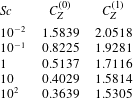
 and
 were found to depend on the Schmidt number over the range
 , which is presented in table 1.
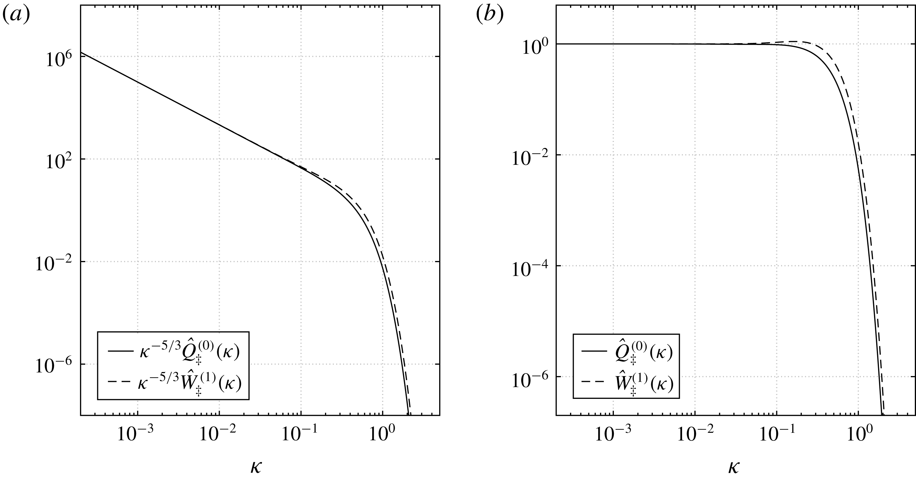
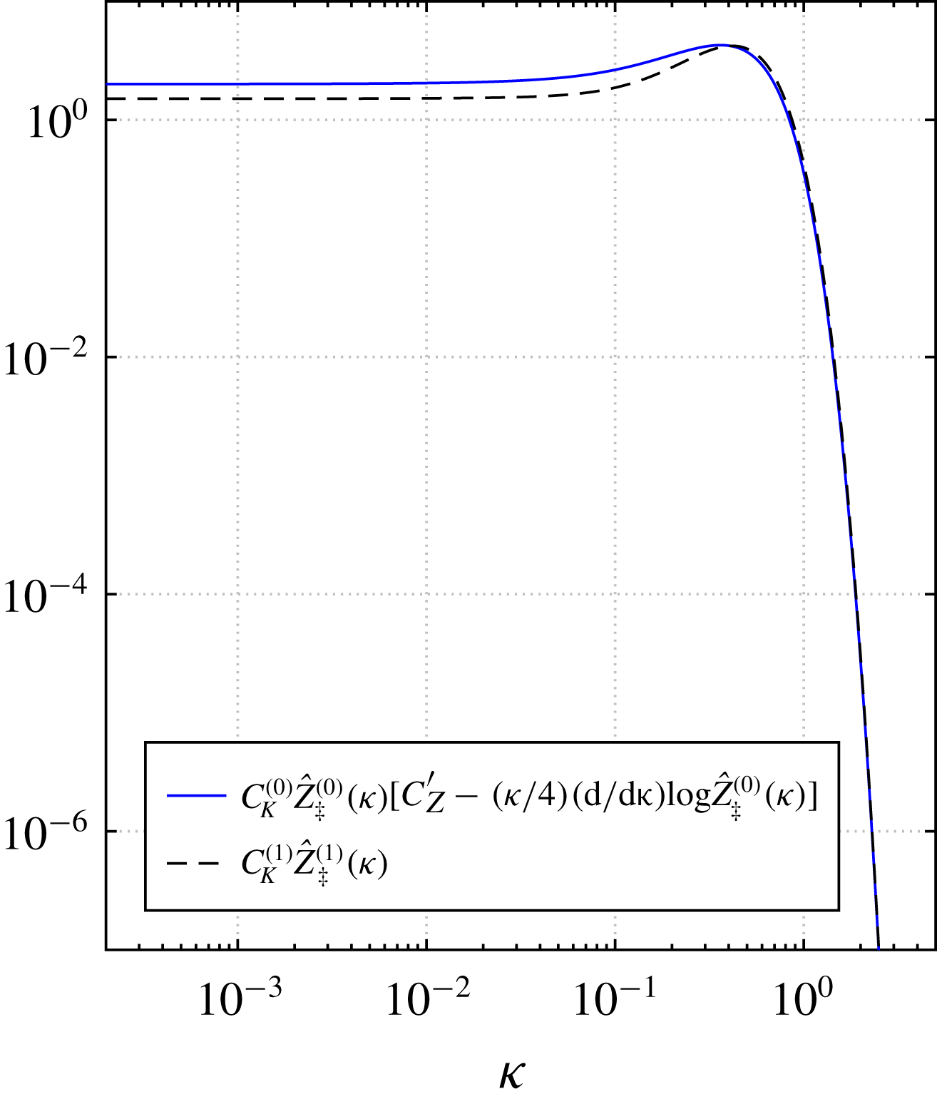
Uncompensated (a) and compensated (b) turbulence kinetic energy spectra as a function of normalised wavenumber.

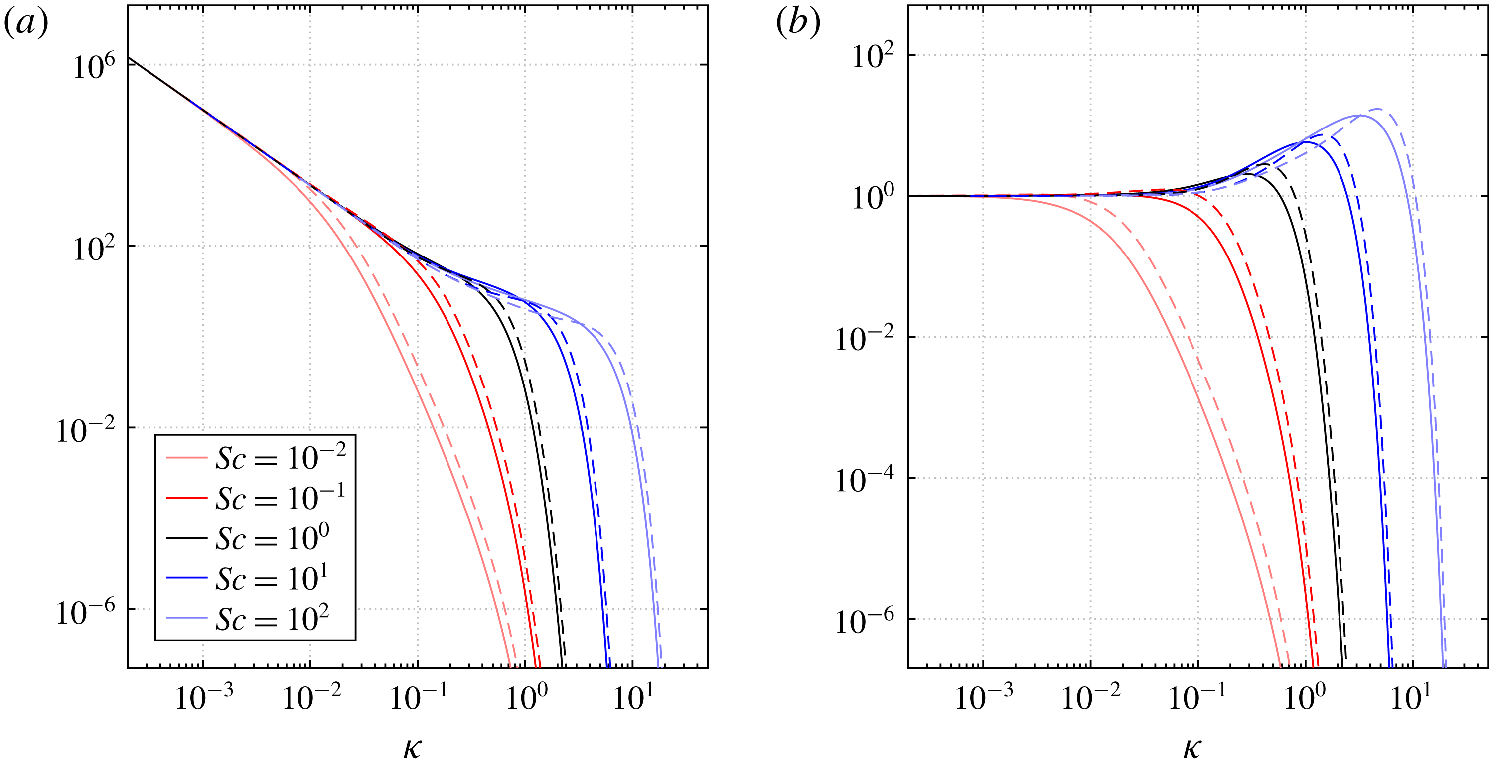
Uncompensated (a) and compensated (b) scalar variance spectra for various
 $Sc$
as a function of normalised wavenumber. Continuous and broken curves denote
 $\hat{Z}_{\ddagger }^{(0)}$
and
 $\hat{Z}_{\ddagger }^{(0)}$
, respectively.

Summary of predicted Obukhov–Corrsin constants for Schmidt number over the ranges
 $Sc\in [10^{-2},10^{2}]$
.

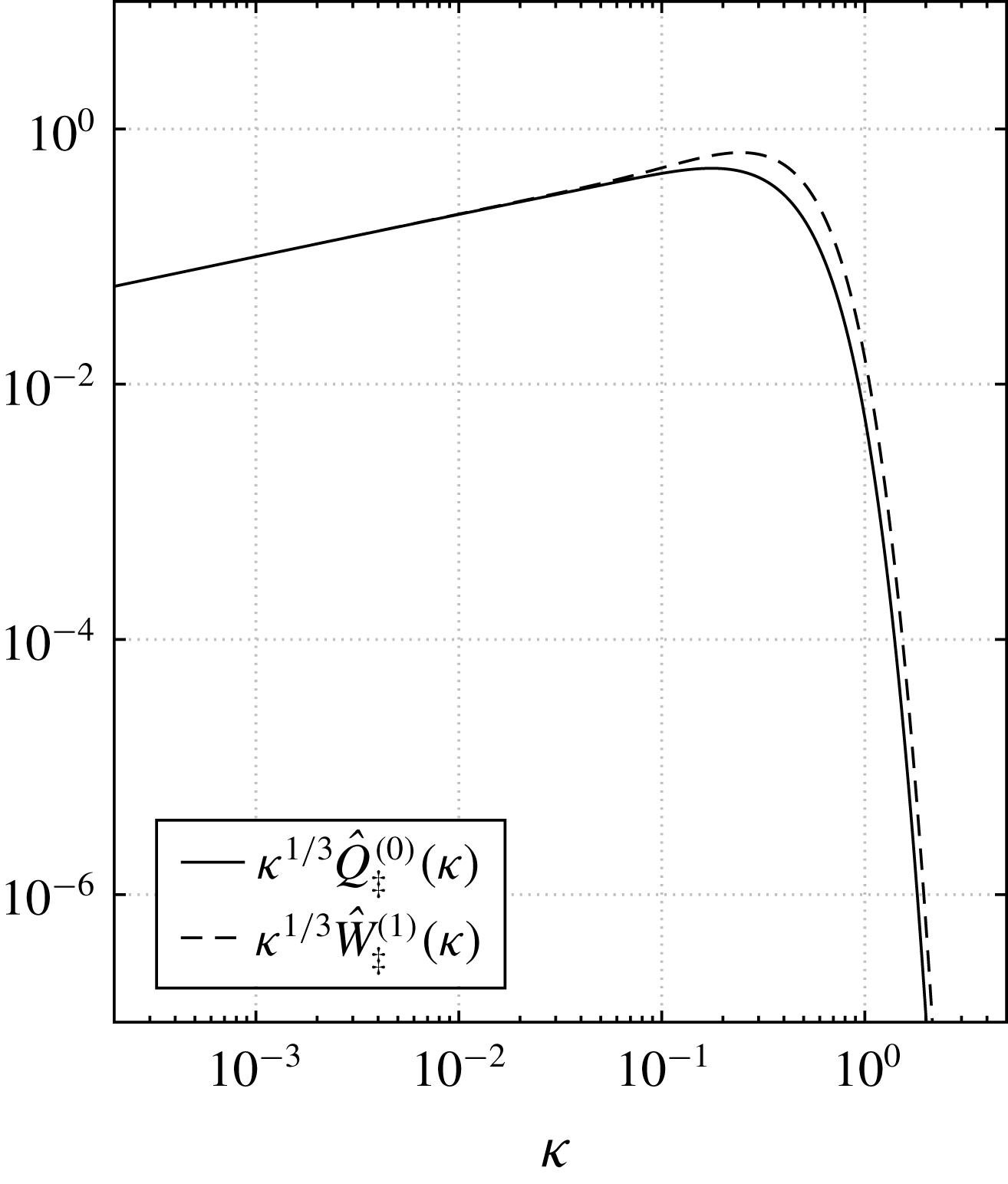
Self-similar turbulence enstrophy spectra.

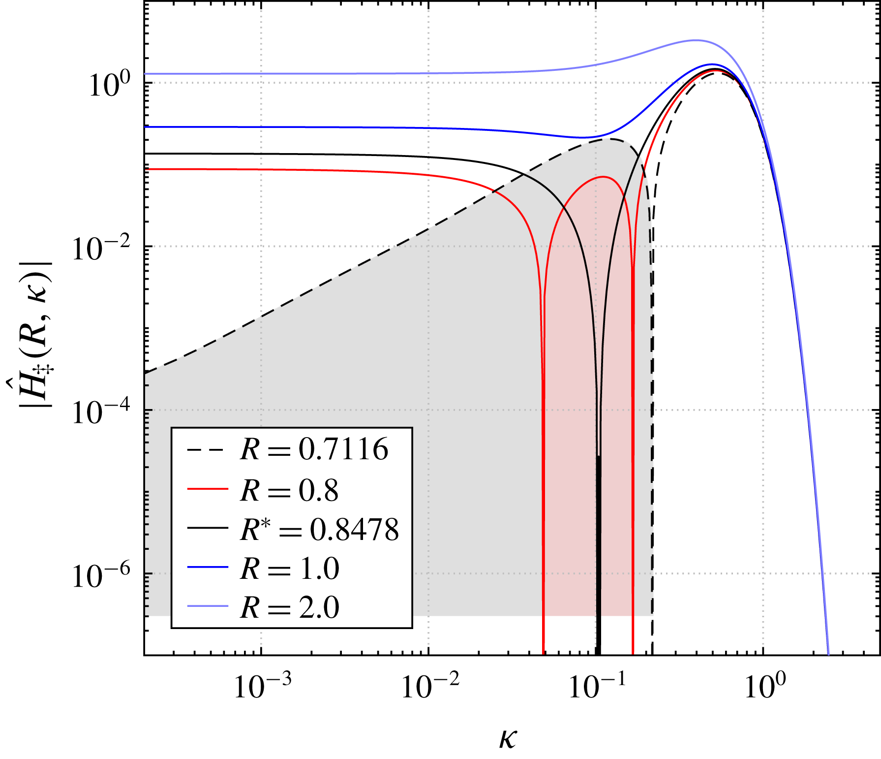
Absolute value of the
 $O(\unicode[STIX]{x1D6FC})$
compensated scalar-variance spectra, second term on the right-hand side of (5.23), for
 $Sc=1.0$
. Shaded regions highlight where this term becomes negative, reducing the overall scalar-variance spectrum.

A comparison of the predicted energy and scalar-variance spectra is shown in figures 1 and 2. It is observed that apart from small differences near the dissipation subrange, the two velocity correlation functions,  and
 , are very similar. This can be interpreted as an indication that the physical mechanisms that govern
 and
 are essentially the same under the assumptions of the SDIP theory. The situation for the scalar spectra,
 and
 , is again the same when appropriately normalised. In both
 $O(\unicode[STIX]{x1D6FC})$
spectra the dissipation subrange expands slightly further to higher wavenumbers, as observed on the right-hand side of figures 1 and 2. This is more evident in the turbulence enstrophy spectra of orders
 $O(1)$
and
 $O(\unicode[STIX]{x1D6FC})$
shown in figure 3. More interesting effects due to variable density can be observed if one plots the total
 $O(\unicode[STIX]{x1D6FC})$
contribution to the scalar variance spectrum,
 in (5.23), as a function of
 $R$
, shown in figure 4. The first appearance of negative values in the
 $O(\unicode[STIX]{x1D6FC})$
scalar-variance spectrum occurs when
 $R=R^{\ast }$
, at the wavenumber
 $\unicode[STIX]{x1D705}=\unicode[STIX]{x1D705}^{\ast }$
from the conditions
 ${\hat{H}}_{\ddagger }=\unicode[STIX]{x2202}{\hat{H}}_{\ddagger }/\unicode[STIX]{x2202}\unicode[STIX]{x1D705}=0$
. This corresponds to
 $R^{\ast }\simeq 0.8478$
and
 $\unicode[STIX]{x1D705}^{\ast }\simeq 0.1043$
. The negativity of this term strengthens for
 $R<R^{\ast }$
over a range of wavenumbers near
 $\unicode[STIX]{x1D705}^{\ast }$
. The region of
 ${\hat{H}}_{\ddagger }$
exhibiting negative values extends all the way into the large scales,
 , under the condition
 , corresponding to
 for
 . The total scalar-variance spectrum must remain positive for all wavenumbers, which places a limit on the extent of this subtractive behaviour. It is likely that for larger values of
 $\unicode[STIX]{x1D6FC}$
, higher-order terms of the asymptotic expansion are additive and must be retained in the case of
 $R$
being sufficiently small. The spectrum adopts a more traditional form for larger values of
 $R$
, as supported by DNS to be discussed below.
6 Comparison to direct numerical simulations
Direct numerical simulations of the zero-Mach variable-density Navier–Stokes equations, equations (2.3)–(2.5), were performed to compare with the SDIP spectral theory in isotropic homogeneous conditions.
6.1 Numerical method
The governing equations are discretised in space using fast Fourier transform (FFT) in a domain
 $[0,2\unicode[STIX]{x03C0}]^{3}$
and integrated in time using an Adams–Bashforth/Crank–Nicolson scheme (explicit treatment of advection and implicit treatment of viscous and diffusion terms). The important parameters of the simulations are listed in table 2. The DNS are restricted to
 $Sc=1$
since the state relationship, equation (2.1), is most applicable for gases with near unity Schmidt numbers. These simulations are isotropic, homogeneous and statistically stationary thanks to a forcing mechanism denoted in the governing equations by
 $f_{l}$
and
 $g$
in (2.3) and (2.4), respectively. The narrow-band forcing is concentrated at the discrete wavemode
 , it is solenoidal, and all simulations of a particular resolution used an identical realisation of the forcing parameters to allow comparisons between simulations. The method used to generate the forcing is described in Yu & Bai (Reference Yu and Bai2014). Furthermore, the parameter
 $\unicode[STIX]{x1D6FC}$
was varied between
 $0$
and
 $-1$
to explore the impact of variable density in the spectra;
 $\unicode[STIX]{x1D6FC}$
is here negative to conform with standard practice in reacting flow but the analysis is equally applicable to positive values. Observe that the microscale Reynolds number varies slightly between simulations of the same resolution (despite having identical forcings in space and time) owing to the variations in density between cases.
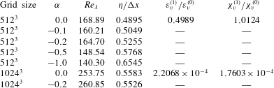
Summary of DNS simulations.

6.2 Statistics
In the case of variable-density flow, it must be recognised that the turbulence kinetic energy dissipation rate is a function of
 $\unicode[STIX]{x1D6FC}$
,
 . This presents some choice when performing a normalisation of the spectra. According to (5.14), the desired value for normalisation is
 , and the factor affecting the leading-order variable-density effect is the dissipation ratio listed in table 2. The main objective of the simulations is the estimation of


and the comparison of the simulation spectra with those predicted by the theory. The main difficulty of calculating these statistics from the variable-density DNS is that one obtains the complete fields
 $\boldsymbol{u}$
and
 $\unicode[STIX]{x1D719}$
, not the expansion fields
 $\boldsymbol{u}^{(0)}$
,
 $\boldsymbol{u}^{(1\text{s})}$
,
 $\unicode[STIX]{x1D719}^{(0)}$
and
 $\unicode[STIX]{x1D719}^{(1)}$
. The governing equations for the expansion fields are always well defined (independently of
 $\unicode[STIX]{x1D6FC}$
), and were the basis of the theoretical development; see (4.6)–(4.7), respectively. The zeroth-order fields derive their energy from the large-scale forcing, while the first-order fields derive their energy from the zeroth-order fields, and so on for higher-order quantities. It is however possible to estimate the above statistics without solving for the perturbation fields. Starting from the governing equations for
 ,
 ,
 and
 in physical space, multiplying the corresponding zeroth-order equation by the first-order field and vice versa and assuming statistical homogeneity, the balance law for
 is given by

where
 $\unicode[STIX]{x1D6FB}^{2}G=g$
and the balance law for
 is given by

The process to arrive at these equations is integration by parts and elimination of terms that involve divergence of averages. The only terms in (6.3) and (6.4) that are impossible to determine without explicit knowledge of  and
 are the
 and
 . Nevertheless, it is expected that the correlations of the forcing functions with the first-order fields are very small,
 and
 , as these fields are driven by the zeroth-order fields. These approximations and statistical stationarity allow estimation of
 and
 purely from the zeroth-order quantities, which can be determined from a constant-density simulation, which is all that is needed to arrive at

and

from (6.3) and (6.4), respectively. Table 2 shows the ratio of the first- to zeroth-order kinetic energy and scalar dissipations after the simulations achieve steady state. For the purposes of comparison to the theoretical predictions, equation (5.23), the
 $512^{3}$
and
 $1024^{3}$
simulations achieve
 $R\simeq 2.3191$
and
 $R\simeq 0.9115$
, respectively. This indicates that one should not expect the
 $O(\unicode[STIX]{x1D6FC})$
contribution of the scalar spectra of the present variable-density DNS to be negative. There is no expectation that the values of the dissipation ratios obtained from the DNS, and consequently
 $R$
, are universal. It is suspected that the amount of energy transferred to the
 $O(\unicode[STIX]{x1D6FC})$
fields depends on the conditions that generate and drive the large scales of the turbulence, specifically the scalar driving force. This can be seen in the fact that
 $g$
enters in (6.5)–(6.6) explicitly. In consequence, the possibility of alternative forcing mechanisms that can induce a subtractive
 $O(\unicode[STIX]{x1D6FC})$
contribution of the scalar spectra cannot be ruled out from the present results.
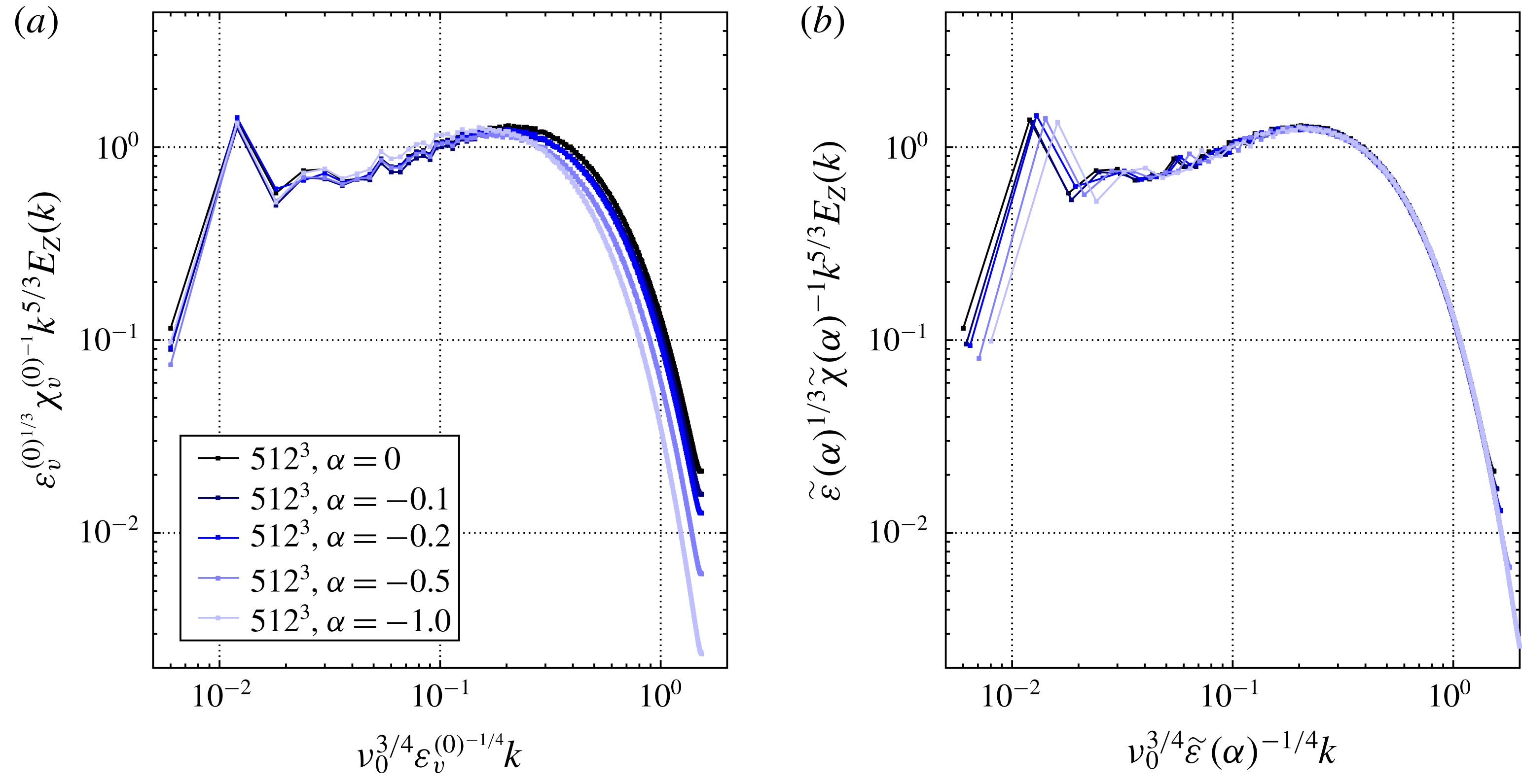
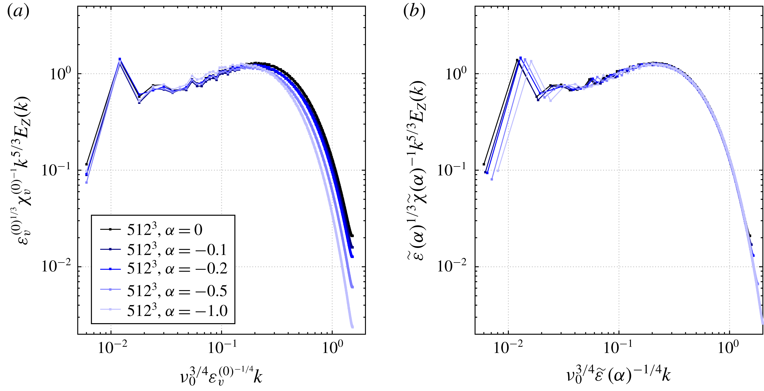
Compensated turbulence kinetic energy spectra of
 $512^{3}$
DNS normalised with: (a)
 $\unicode[STIX]{x1D700}_{v}^{(0)}$
, and (b)
 $\tilde{\unicode[STIX]{x1D700}}(\unicode[STIX]{x1D6FC})$
.

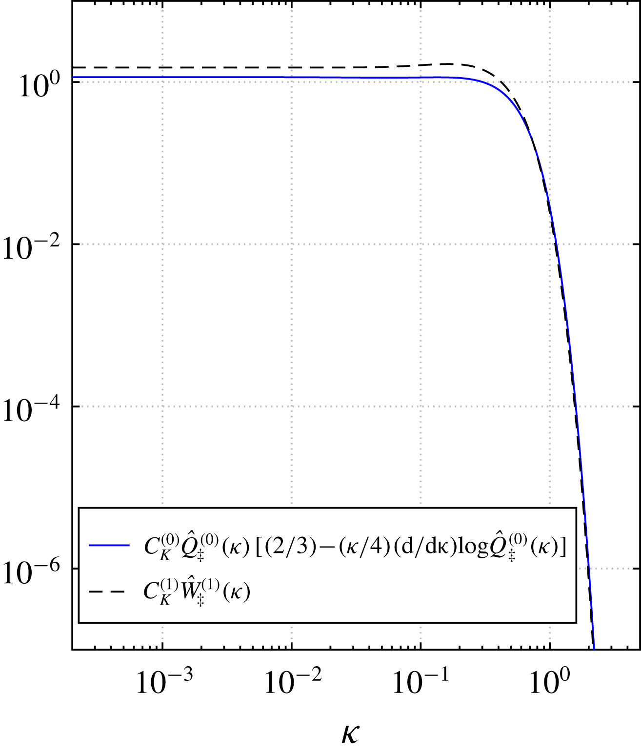
Comparison of normalising the turbulence kinetic energy spectra by the Favre dissipation per unit mass with SDIP prediction.

Figure 5(a) shows turbulence kinetic energy spectra of
 $512^{3}$
DNS as a function of
 $\unicode[STIX]{x1D6FC}$
using
 . It is observed that the changes of the energy spectra (with respect to the constant-density flow) are small for small
 $\unicode[STIX]{x1D6FC}$
but they increase for larger values. The overall shape of the spectra does not change for small
 $\unicode[STIX]{x1D6FC}$
, since
 and
 are very similar; see figure 1. Note that one may find a situation, for
 $\unicode[STIX]{x1D6FC}\sim -1$
, where the two fundamental spectra cancel each other within the inertial subrange but lead to large differences within the dissipation subrange. But it may be premature to extrapolate to these large values of
 $\unicode[STIX]{x1D6FC}$
since the current expansion is limited to
 $\unicode[STIX]{x1D6FC}$
small. Next, figure 5(b) shows that normalising by the Favre dissipation per unit mass,
 , tends to collapse the effect of
 $\unicode[STIX]{x1D6FC}$
better. This is a feature well documented in experiments and previous simulations (Knaus & Pantano Reference Knaus and Pantano2009; Kolla et al.
Reference Kolla, Hawkes, Kerstein, Swaminatham and Chen2014) but without any formal theoretical justification. The essential implication is that variable-density turbulence kinetic energy spectra, for arbitrary
 $\unicode[STIX]{x1D6FC}$
, is well described by the following approximation

Performing an expansion of the right-hand side of (6.7) in terms of
 $\unicode[STIX]{x1D6FC}$
about the constant-density limit, and equating the
 $O(\unicode[STIX]{x1D6FC})$
term to that which appears in (5.14) results in the following relationship

A comparison of the left- and right-hand sides of (6.8) is shown in figure 6. The SDIP theory replicates the observed trend to a high degree of accuracy in the dissipation subrange. In the inertial subrange however, the left-hand side of (6.8) asymptotes to  as
 , whereas the right-hand side tends to
 . This discrepancy may be the manifestation of a small error in the approximations used to derive the two-time velocity correlations and Lagrangian velocity–velocity response which is more apparent in the case of the scalar statistics. The perturbative approach used in this work highlights that there is a substantial effect induced by variable density, but this is hidden when the spectra are scaled with
 ; to differentiate the effect that variable density introduces in the flow one should use the reference constant-density value for normalisation. A direct comparison of the theoretically predicted turbulence kinetic energy spectra with those calculated from
 $1024^{3}$
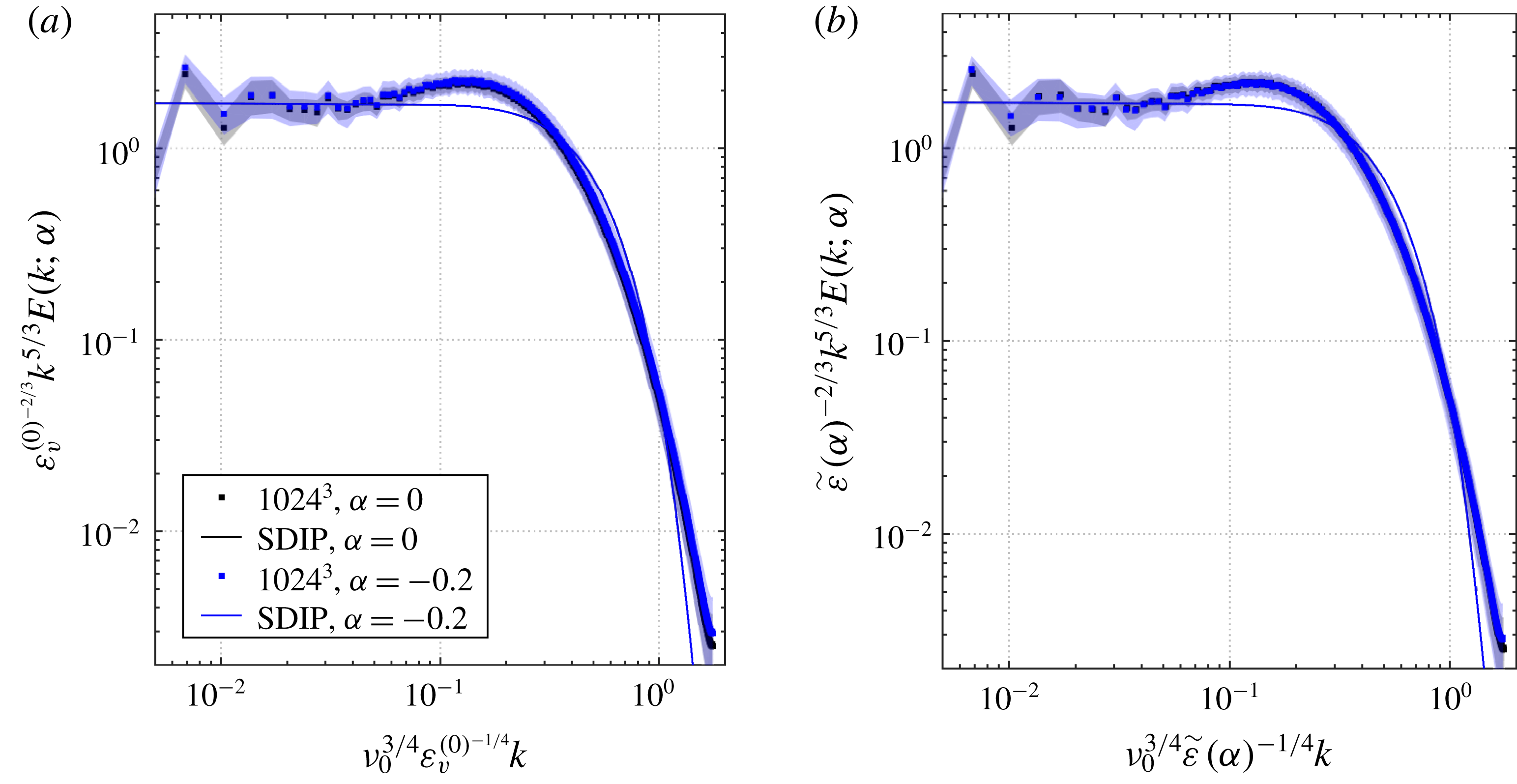
DNS is shown in figure 7. The dissipation ratios for these simulations were calculated to be much smaller than the
 $512^{3}$
, and consequently the effect of variable density is minimal. The difference between the
 $512^{3}$
and
 $1024^{3}$
dissipation ratios comes from variations in the forcing parameters but primarily from the larger Reynolds number of the latter. From the limited simulation results, it appears that the ratio of dissipations is strongly affected by Reynolds number such that the energy transfer to the
 $O(\unicode[STIX]{x1D6FC})$
fields reduces substantially with increasing Reynolds numbers. Note that figure 7 also shows (shaded areas) the confidence interval (95 % variation) of the statistically averaged spectra. In this representation, one observes a somewhat larger variability of the confidence spectra within the inertial subrange for the variable-density flow, in comparison with the constant-density flow. This is consistent with recent observations using wavelet analysis of reacting flame spectra by Kim et al. (Reference Kim, Bassenne, Towery, Hamlington, Poludnenko and Urzay2018).
Compensated turbulence kinetic energy spectra of
 $1024^{3}$
DNS normalised with
 $\unicode[STIX]{x1D700}_{v}^{(0)}$
(a), and
 $\tilde{\unicode[STIX]{x1D700}}(\unicode[STIX]{x1D6FC})$
(b). Shaded regions highlight the 95 % sampling confidence interval of the spectra.

Compensated scalar-variance spectra for
 $Sc=1$
of
 $512^{3}$
DNS normalised with: (a)
 $\unicode[STIX]{x1D700}_{v}^{(0)}$
and
 $\unicode[STIX]{x1D700}_{v}^{(0)}$
, and (b)
 $\tilde{\unicode[STIX]{x1D700}}(\unicode[STIX]{x1D6FC})$
and
 $\tilde{\unicode[STIX]{x1D712}}(\unicode[STIX]{x1D6FC})$
.

Comparison of normalising the scalar-variance spectra by the Favre dissipation per unit mass with SDIP prediction.

The
 $512^{3}$
DNS scalar spectra are shown in figure 8(a) for different values of
 $\unicode[STIX]{x1D6FC}$
. As with the turbulence kinetic energy spectra, small changes to the scalar spectra are observed for small
 $\unicode[STIX]{x1D6FC}$
and much larger changes are observed for the highest value of
 $\unicode[STIX]{x1D6FC}$
that was simulated. Figure 8(b) shows a similar collapse of the scalar spectra when normalising by the Favre dissipation per unit mass. Following the same procedure used to derive (6.8), comparison of scalar spectra
 $O(\unicode[STIX]{x1D6FC})$
terms with (5.23) results in the following relationship:

where  . A comparison of the left- and right-hand sides of (6.9) are shown in figure 9. As with the turbulence kinetic energy spectra, the dissipation subrange trend is replicated by the SDIP theory, but an offset is observed in the inertial subrange; the left-hand side of (6.9) asymptotes to
 as
 , whereas the right-hand side tends to
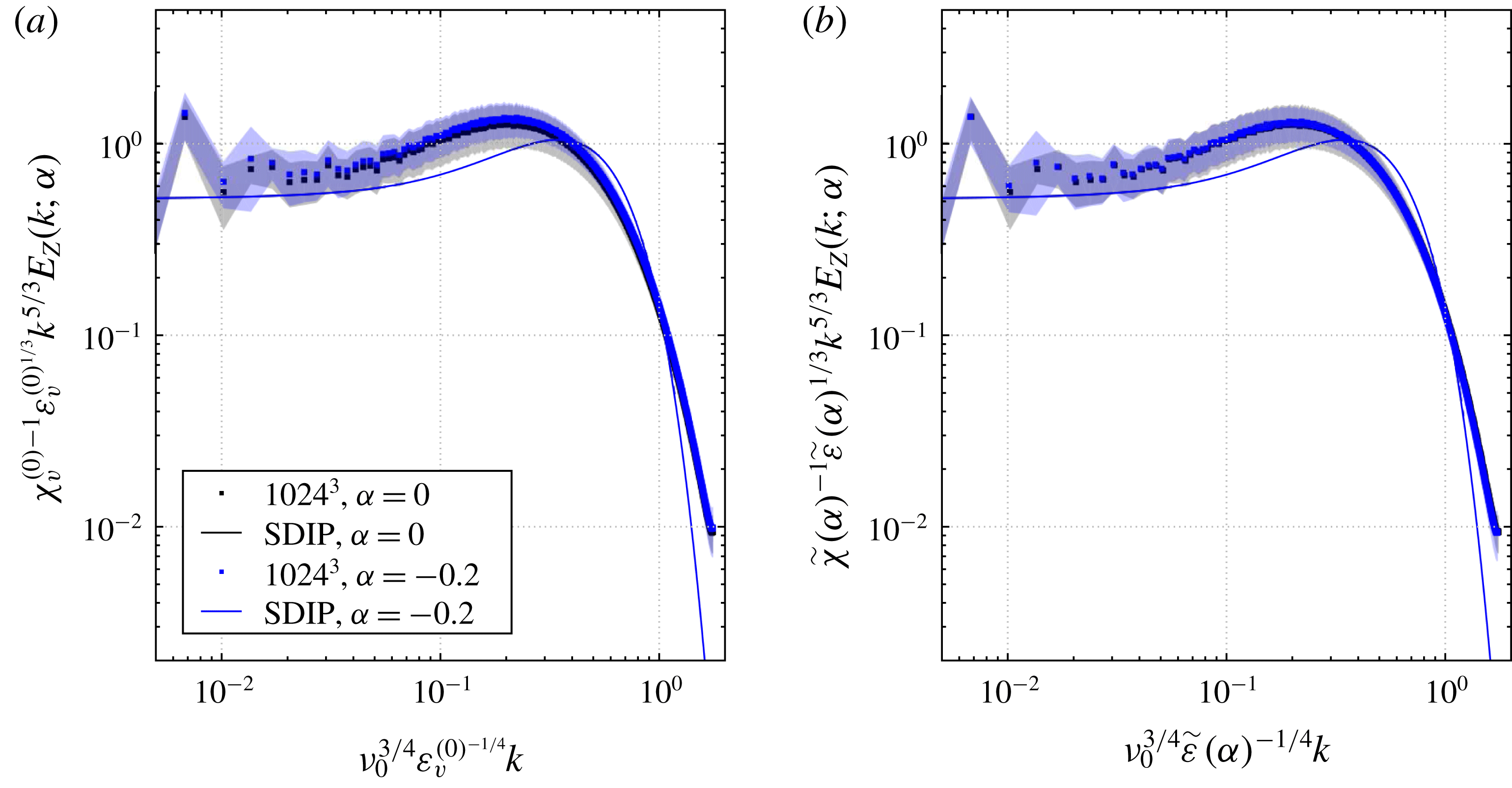
 . A direct comparison of the theoretically predicted turbulence scalar spectra with those calculated from
 $1024^{3}$
DNS is shown in figure 10. As with the
 $1024^{3}$
DNS turbulence kinetic energy spectra, the variable-density effects on the
 $1024^{3}$
DNS scalar spectra are minimal due to small dissipation rate ratios.
Compensated scalar-variance spectra for
 $Sc=1$
of
 $1024^{3}$
DNS normalised with
 $\unicode[STIX]{x1D700}_{v}^{(0)}$
and
 $\unicode[STIX]{x1D712}_{v}^{(0)}$
(a), and
 $\tilde{\unicode[STIX]{x1D700}}(\unicode[STIX]{x1D6FC})$
and
 $\tilde{\unicode[STIX]{x1D712}}(\unicode[STIX]{x1D6FC})$
(b). Shaded regions highlight the 95 % sampling confidence interval of the spectra.

As a summary, there are at least three clear ways in which the DNS spectra can be modified. First, for divergence-free forcing, the scalar spectra can be modified by inducing smaller values of  in comparison to the reported values of the present simulations. In that case, the scalar spectra may develop the anti-correlation shown in figure 4 and that will alter markedly the form of the dissipative subrange of the total scalar spectrum. Several variations of the forcing parameters did not achieve scalar spectrum anti-correlation, which was not the goal of this study, and therefore it remains open to speculation whether this behaviour is possible in a real turbulent flow. Second, under the perturbative approach presented earlier, momentum forcing has to be solenoidal. Non-solenoidal forcing will produce disordering of the current asymptotic expansion (since no divergence-free solution would exist for constant density) but it may be admissible to develop a different expansion that can accommodate this type of forcing. Third, and finally, the presence of either a velocity or scalar gradient will alter the spectral energy interactions in a manner that is difficult to predict at this point because the SDIP derivations become overly difficult. It is expected that the inertial subrange is modified anisotropically under a mean temperature gradient, and the flux spectrum still decays as
 $k^{-7/3}$
, as predicted by Lumley (Reference Lumley1964), but the changes around and in the dissipation subrange are likely going to be different from those described presently.
7 Conclusion
In this work, a second-order statistical closure of variable-density homogeneous stationary isotropic turbulence has been derived. The flow is assumed to obey the zero-Mach variable-density equations, with an ideal gas thermal state relationship. An asymptotic expansion about the incompressible limit is taken to identify the first-order variable-density effects upon the statistical quantities of interest. Statistical closure is addressed using the sparse direct-interaction approximation, which does not introduce ad hoc parameters requiring calibration. The resulting theory predicts that density variation minimally affects the turbulence kinetic energy spectra, as it is often observed in practical flows. In contrast, the theory predicts that for certain types of large-scale dynamics, it is possible to induce anti-correlation in the scalar spectra, which has been characterised using ratios of turbulence and scalar dissipation rates as the global parameters controlling the large-to-small scale energy fluxes. In addition, a new treatment of the two-time scalar correlation and response functions of the SDIP theory shows an improvement of the predicted Obukhov–Corrsin constant. The new treatment explicitly exposes the dependence of some scalar statistics on the velocity correlation, which was not present in previous closures. The governing equations produced by the presently extended SDIP theory of turbulence are solved by an integro-differential numerical method and the leading (constant density) results are confirmed by comparison with previously published values. The next-order (variable density) results were obtained here for the first time.
Complementary direct numerical simulations of turbulence with differing levels of density variations have been performed. The resulting spectra of these simulations have been compared to the theoretically derived closures. The analysis indicates that the constant-density volumetric dissipation is the proper scaling for comparison of spectra with different levels of density variation. It is also shown that the usual scaling of the energy and scalar-variance spectra using Favre-based dissipation rates per unit mass do collapse the data for various levels of density variation. Reinterpretation of the present theory is supportive of this observation. The agreement is excellent within the dissipation subrange for all levels of density variation considered.
Acknowledgements
This work was supported in part by the Air Force Office of Scientific Research under grant no. FA9550-15-1-0035 (Dr C. Li, Program Manager) and by the Department of Energy, National Nuclear Security Administration, under award no. DE-NA0002382, and the California Institute of Technology.
Appendix A. Incompressible spectral governing equations
The constant-density
 $O(1)$
primitive spectral fields evolve, see Kida & Goto (Reference Kida and Goto1997) and Goto & Kida (Reference Goto and Kida1999), according to

and

with mass constraint

and the
 $O(1)$
spectral modified pressure is defined as

The
 $O(1)$
Lagrangian map evolves according to

and satisfies the initial condition

The
 $O(1)$
spectral Lagrangian velocity is defined by the following mapping

which evolves according to

and where  . The
 $O(1)$
spectral Lagrangian scalar is defined by the following mapping

which evolves according to

and where  . The
 $O(1)$
semi-Lagrangian velocity correlation, where
 , is defined as

where  and the solenoidal property of
 $\tilde{u} _{j}^{(0)}$
requires that
 . The
 $O(1)$
first semi-Lagrangian scalar flux, where
 , is defined as

where the solenoidal property of
 $\tilde{u} _{j}^{(0)}$
requires that
 . The
 $O(1)$
second semi-Lagrangian scalar flux, where
 , is defined as

The
 $O(1)$
semi-Lagrangian scalar correlation, where
 , is defined as

where  .
Appendix B. Incompressible sparse direct-interaction perturbation
The
 $O(1)$
instantaneous semi-Lagrangian velocity correlation evolves according to

and the
 $O(1)$
two-time semi-Lagrangian velocity correlation, where
 , evolves according to

Applying the SDIP methodology to (B 1) results in

and to (B 2) gives

The
 $O(1)$
ensemble Lagrangian–Eulerian velocity–velocity response, where
 , is defined as

which evolves according to

and satisfies the initial condition  . The pressure response term is given by

Applying the SDIP methodology to (B 6) results in

The
 $O(1)$
two-time semi-Lagrangian scalar-velocity correlation evolves according to

with initial condition  . Applying the SDIP methodology to the
 $O(1)$
two-time semi-Lagrangian scalar-velocity correlation governing equation results in

The
 $O(1)$
instantaneous semi-Lagrangian scalar correlation evolves according to

and the
 $O(1)$
two-time semi-Lagrangian scalar correlation, where
 , evolves according to

Applying the SDIP methodology to (B 11) results in

Applying the proposed alternative approximation, based upon the Taylor series expansion of the
 $O(1)$
Lagrangian scalar, to (B 12) gives

The
 $O(1)$
ensemble Lagrangian–Eulerian scalar–scalar response, where
 , is defined as

which evolves according to

and satisfies the initial condition  . Similarly to the derivation of (B 14), the proposed alternative approximation of the
 $O(1)$
Lagrangian scalar produces

Applying the condition of statistical isotropy restricts the tensorial statistical quantities to be defined as

where the mass constraint requires  . Applying these statistical restrictions to (B 3) gives

and to (B 4) gives

Similarly, application of these restrictions to (B 6) gives

with initial condition  . It follows from (B 21) that integration of (B 20) with respect to
 results in

Asserting statistical isotropy reduces (B 10) to

with initial condition  . Consequently, the trivial solution
 applies and henceforth the
 $O(1)$
spectral scalar-velocity correlation will be disregarded.
Statistical isotropy applied to (B 11) gives

and to (B 12) gives

Applying the condition of statistical isotropy to (B 17) gives

with initial condition  . Integrating with respect to


It follows from (B 26) that integration of (B 25) with respect to  results in

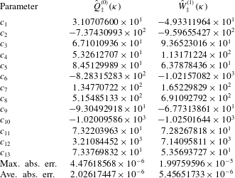
Coefficients and fit errors of
 $\hat{Q}_{\ddagger }^{(0)}(\unicode[STIX]{x1D705})$
and
 ${\hat{W}}_{\ddagger }^{(1)}(\unicode[STIX]{x1D705})$
approximants.

Appendix C. Padé-like approximants of the spectra
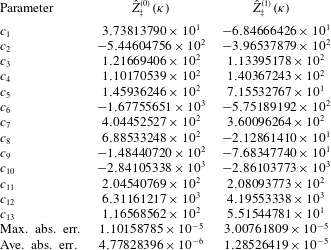
Padé-like approximants of the converged solutions generated by the integro-differential SDIP solver are presented for completeness. The spectra were fitted to the generic form

where the coefficients and fit errors for  and
 are reported in table 3, as well as
 and
 for
 in table 4. The rational polynomial in front of the exponential term predominantly controls the shape of the spectra in the inertial sub-range. The rational polynomial within the exponential predominantly controls the spectrum shape in the dissipation sub-range. This form is crucial to achieve the quoted accuracy in tables 3–4 over the entire range of wavenumbers. These approximants reproduce the quoted values of the associated Kolmogorov or Obukhov–Corrsin constants in § 5.
The unity boundary condition is recovered in all cases when  . The asymptotic behaviour of the spectra at large wavenumbers is given by

which is a simple approximation of the spectra in the dissipation sub-range.
Coefficients and fit errors of
 $\hat{Z}_{\ddagger }^{(0)}(\unicode[STIX]{x1D705})$
and
 $\hat{Z}_{\ddagger }^{(1)}(\unicode[STIX]{x1D705})$
approximants for
 $Sc=1$
.