2.1 Experimental method and model

The uniform flexible cylinder model has a diameter $d=0.5~\text{cm}$ and a length $L=120~\text{cm}$ , with a resulting aspect ratio of 240. The model is constructed/moulded via urethane rubber (density of $1.38~\text{g}~\text{cm}^{-3}$ ) mixed with tungsten (density of $19.3~\text{g}~\text{cm}^{-3}$ ) powder in order to reach a mass ratio of $m^{\ast }=4.0$ (the ratio between structural mass to displaced fluid mass). In addition, a fishing line is embedded in the centre during the moulding process to provide sufficient axial stiffness. In the current experiment, the effect of the bending stiffness on the model’s natural frequency and modal shape is negligible, compared to that of the tensions applied. Note that the structural damping of the urethane rubber material is higher than the traditional metal or ABS plastic cylinder model. Nonetheless, the damping ratio of the current flexible model is $8.7\,\%$ , as obtained from the pluck test in the air.

We performed systematic experiments at the MIT tow tank facility with a water depth of 1.22 m. An aluminium frame was built to provide mounting points for the bottom of the model and a ‘6-axis ATI Gamma’ sensor was installed on top of the frame in order to measure the model’s top tension in each experimental run. The vertically installed model had a 97 % total immersion length, and it was clamped at both ends. The model was towed to generate a uniform inflow with different speeds from 0.05 to $0.46~\text{m}~\text{s}^{-1}$ , achieving Reynolds numbers $Re$ from 250 to 2300 while the reduced velocity varied from 4.8 to 36. Here, the reduced velocity $U_{r}$ and the true reduced velocity $V_{r}$ are defined as follows:

(2.1) $$\begin{eqnarray}\left.\begin{array}{@{}c@{}}\displaystyle U_{r}=\frac{U}{f_{n1}d},\\ \displaystyle V_{r}=\frac{U}{f_{y}d},\end{array}\right\}\end{eqnarray}$$

where $U$ is the inflow velocity, $d$ is the model diameter, $f_{n1}$ is the first modal natural frequency, calculated based on the measured tension, assuming $C_{m}=1.0$ along the model, and $f_{y}$ is the actual vibration frequency measured in the CF direction. Figure 2 shows a sketch of the experimental set-up, while table 1 lists the experimental parameters.

We applied our newly developed underwater optical methods using eight high-speed cameras to capture the IL and CF vibrations for a total of 52 locations (staggered black and white markers) along the model. Compared to the traditional strain-gauge and accelerometer measurement for flexible cylinder VIV experiments, the optical tracking system provides both temporally and spatially dense and direct measurements on the model displacement response (Fan, Du & Triantafyllou Reference Fan, Du and Triantafyllou2016). Three cameras are installed over 160 $d$ downstream of the model to measure the CF vibration while five cameras are installed 100 $d$ besides the model to measure the IL vibration. At the same time, four 1500-lumen underwater lights were installed to provide enough camera background lighting. Corresponding image processing and motion tracking code were developed to capture and follow the trajectory of either white or black markers (Fan & Triantafyllou Reference Fan and Triantafyllou2017). Figure 2(b) displays a sample frame of the raw and processed images for one of the cameras. More details about the camera set-up and the image process method are described in appendix A.

2.2 Numerical method and model

In order to obtain a quantitative understanding of the complex vortex shedding process, we carried out a large-eddy simulation (LES) study by using the entropy-viscosity method, which was proposed by Guermond, Pasquetti & Popov (Reference Guermond, Pasquetti and Popov2011a ,Reference Guermond, Pasquetti and Popov b ) and later developed further for complex flows in Wang et al. (Reference Wang, Triantafyllou, Constantinides and Karniadakis2018, Reference Wang, Triantafyllou, Constantinides and Karniadakis2019). In the simulation, the governing equations of the incompressible flow are solved by a Fourier/spectral-element code that employs spectral-element discretization in the ( $x$ – $y$ ) plane and Fourier expansion along the riser axial direction ( $z$ ) as presented in Karniadakis & Sherwin (Reference Karniadakis and Sherwin2005). The coordinate transformation method proposed in Newman & Karniadakis (Reference Newman and Karniadakis1997) is employed to deal with the boundary deformation due to the vibration. On the ( $x$ – $y$ ) plane, the computational domain has a size of $[-6.5d,23.5d]\times [-20d,20d]$ , which is partitioned into $2\,616$ quadrilateral elements, where $d=1$ is the cylinder diameter whose centre is placed at $(0,0)$ . On the left boundary of the domain where $x/d=-6.5$ , $u=U,v=0,w=0$ are imposed, where $u,v,w$ are the three components of velocity vector $\boldsymbol{u}$ ; on the right boundary where $x/d=23.5$ , $p=0$ and $\unicode[STIX]{x2202}\boldsymbol{u}/\unicode[STIX]{x2202}\boldsymbol{n}=0$ are prescribed, where $p$ is the pressure and $\boldsymbol{n}$ is the normal vector; on both top and bottom boundaries where $y/d=\pm 20$ , a periodic boundary condition is used.

Figure 2.

The flexible model in the MIT tow tank: (a) a sketch of the experimental set-up that shows the uniform incoming flow and the black and white strips used for motion tracking purposes; (b) sample raw (top) and processed (bottom) image shows that the red bounding box captures the motion of the white markers.

Table 1.

Values of the experimental parameters of the uniform flexible model.

The cylinder motion is governed by a linear beam-string equation as follows:

(2.2) $$\begin{eqnarray}\frac{\unicode[STIX]{x2202}^{2}\unicode[STIX]{x1D709}_{J}}{\unicode[STIX]{x2202}t^{2}}+2\unicode[STIX]{x1D701}\unicode[STIX]{x1D714}_{n}\frac{\unicode[STIX]{x2202}\unicode[STIX]{x1D709}_{J}}{\unicode[STIX]{x2202}t}+\frac{EI}{\unicode[STIX]{x1D707}}\frac{\unicode[STIX]{x2202}^{4}\unicode[STIX]{x1D709}_{J}}{\unicode[STIX]{x2202}z^{4}}-\frac{T}{\unicode[STIX]{x1D707}}\frac{\unicode[STIX]{x2202}^{2}\unicode[STIX]{x1D709}_{J}}{\unicode[STIX]{x2202}z^{2}}=\frac{F}{\unicode[STIX]{x1D707}},\end{eqnarray}$$

where $\unicode[STIX]{x1D709}_{J}$ is the displacement in the  $J$ direction ( $J=x$ or $J=y$ ), $\unicode[STIX]{x1D707}$ is the cylinder mass per unit length, the damping coefficient $\unicode[STIX]{x1D701}=8.7\,\%$ is equal to that of experiment with $\unicode[STIX]{x1D714}_{n}=2\unicode[STIX]{x03C0}f_{n1}$ , $T$ is the tension and $EI$ is the bending stiffness. The above equation is constrained by pinned boundary conditions ( $\unicode[STIX]{x1D709}_{J}=0$ and $\unicode[STIX]{x2202}^{2}\unicode[STIX]{x1D709}_{J}/\unicode[STIX]{x2202}z^{2}=0$ ) at both ends. Note that in the simulation, $T=(UL/U_{r}d)^{2}(4\unicode[STIX]{x1D707}+C_{m}\unicode[STIX]{x1D70C}\unicode[STIX]{x03C0}d^{2})$ with $C_{m}=1.0$ , where $U_{r}$ is the corresponding reduced velocity defined in equation (2.1), while the value of $EI$ is set as small as $0.02T$ , in order to mimic a tension dominated riser (see Evangelinos & Karniadakis Reference Evangelinos and Karniadakis1999). $F$ is the $J$ -component of the hydrodynamic force exerted on the cylinder surface, computed from the integral of the pressure and viscous stress terms using the following equation:

(2.3) $$\begin{eqnarray}F=\oint (-p\boldsymbol{n}+\unicode[STIX]{x1D708}(\unicode[STIX]{x1D735}\boldsymbol{u}+\unicode[STIX]{x1D735}\boldsymbol{u}^{T})\boldsymbol{\cdot }\boldsymbol{n}),\end{eqnarray}$$

where the integration is performed around the circumference of the circular cross-section and $\boldsymbol{n}$ is the outward unit normal on the cylinder, $\unicode[STIX]{x1D708}$ is the kinematic viscosity. In order to solve the governing equation (2.2), we have used the second-order central-difference scheme in space and the Runge–Kutta method in time. For all the simulations in this paper, unless mentioned explicitly, a cubic polynomial is used in each element per direction and 512 Fourier planes are used along the axis ( $z$ -direction). For each simulation, the total computational time $tU_{\infty }/d\geqslant 500$ with a time step $\unicode[STIX]{x0394}t=1.5\times 10^{-3}$ . In total, eight simulations using the same parameters as those of the experiments with $Ur$ in the range of $[10.75,17.22]$ were performed. Validation tests on displacements and excited frequencies are presented in appendix E.

3.1 Frequency and displacement response

In figure 3(a), we plot the VIV frequency response of the flexible cylinder at $U=0.19~\text{m}~\text{s}^{-1}$ ( $Ur=18.1$ ). The flexible model vibrates in the CF direction at one single narrow-banded frequency along the entire span. We also see in figure 3(b) that the exact 2nd harmonic vibration dominates the entire model although some low-frequency responses can be spotted in the IL direction. Such vibration patterns of the single narrow-band frequency response in the CF direction and the dominating 2nd harmonic vibration in the IL direction were found consistent in the current experiment.

Figure 3.

Frequency response along the flexible model at $U=0.19~\text{m}~\text{s}^{-1}$ ( $U_{r}=18.1$ ): (a) in the CF direction, the model vibrates within a narrow-band single frequency, and the inset figure plots the CF frequency response at $z/d=-160$ ; (b) in the IL direction, the 2nd harmonic of the vibration dominates the response.

Figure 4.

Experimental results of the displacement response in the CF direction: (a) three-dimensional (3-D) visualization of the displacement response as a function of $z/d$ and $U_{r}$ ; (b) displacement response along the flexible model at $U_{r}=12.7$ , 21.6 and 32.2; (c) displacement response versus $U_{r}$ at locations $z/d=-180$ , $-120$ and $-60$ . Note that the displacement response here is presented based on $1/10$ th highest peak measurement. In the current experiment, as $U_{r}$ increases, the flexible model vibrates at a higher mode number up to 6th mode in the CF direction. The amplitude response along the model span at higher $U_{r}$ is asymmetric, a sign of mixed standing and travelling wave response patterns.

Figure 5.

Experimental results of the displacement response in the IL direction: (a) 3-D visualization of the displacement response as a function of $z/d$ and $U_{r}$ ; (b) displacement response along the flexible model at $U_{r}=12.7$ , 21.6 and 32.2; (c) displacement response versus $U_{r}$ at locations of $z/d=-180$ , $-120$ and $-60$ . Note that the displacement response here is presented based on $1/10$ th highest peak measurement. In the current experiment, as $U_{r}$ increases, the flexible model vibrates at a higher mode number up to 11th in the IL direction. A symmetric amplitude response along the model span is observed in our experiments.

Based on the dominant frequency components from the power spectral density (PSD), the corresponding $1/10$ th highest peak of the IL and the CF displacement along the model is plotted in figures 4(a) and 5(a) against $U_{r}$ . With increasing $U_{r}$ , higher modes are excited in both the IL and the CF directions. In the current experiment, the 1st to 6th CF modes and the 2nd to 11th IL modes are excited. In general, in the CF direction, the results show on average 5–6 times larger displacement response than that in the IL direction.

Furthermore, three different cases of $U_{r}$ ( $U_{r}=12.7$ , $U_{r}=21.6$ and $U_{r}=32.2$ ) are selected to plot the displacement response along the entire model in figure 4(b) for the CF response and figure 5(b) for the IL response. We observe an asymmetric modal displacement response along the span in the CF direction, while in the IL direction, a symmetric sinusoidal mode shape is consistently found. A comparison between the case of $U_{r}=12.7$ and the case of $U_{r}=32.2$ shows that at lower $U_{r}$ , a pure standing wave is observed in the CF direction. In contrast, with the increasing $U_{r}$ , a mixture of standing and travelling wave response gradually appears in the CF direction. As shown in figure 4, the CF displacement response is rather ‘flat’ and no clear node can be easily identified. However, in the IL direction, the model displays a pure standing wave pattern at both low and high $U_{r}$ . In addition, figures 4(c) and 5(c) plot the CF and the IL displacements as a function of $U_{r}$ at three different locations ( $z/d=-168$ , $z/d=-108$ and $z/d=-48$ ) along the model, respectively. At these three locations, both the IL and the CF displacements vary significantly with $U_{r}$ .

Figure 6.

Frequency ratio and maximum amplitude of the CF displacement along the span versus $U_{r}$ . Red stars, frequency ratio $f_{y}/f_{n1}$ ; blue diamonds, maximum amplitude of the CF displacement. Cases in the same modal group (same dominant mode in both the IL and the CF directions) are labelled together with the black dashed arrow. Starting from $U_{r}=8.84$ , in the same modal group the maximum of $A_{y}/d$ monotonically increases with $U_{r}$ , but during the modal group switch, both the maximum of $A_{y}/d$ and the frequency ratio $f_{y}/f_{n1}$ jump. The $f_{y}/f_{n1}$ of the ‘ $2n:n$ ’ modal group highlighted by the black box, for example modal group ‘ $6/3$ ’, shows that the actual vibration frequency is larger than the natural modal frequency predicted in still water.

Figure 7.

Frequency ratio and maximum amplitude of the IL displacement along the span against $U_{r}$ . Red stars, frequency ratio $f_{x}/f_{n1}$ ; blue diamonds, maximum amplitude of the IL displacement. Starting from $U_{r}=8.84$ , in the same modal group the maximum of $A_{x}/d$ monotonically increases with $U_{r}$ , but during the modal group switch, both the maximum of $A_{x}/d$ and the frequency ratio $f_{x}/f_{n1}$ jump.

From figures 4(a) and 5(a), the maximum amplitudes of the IL and the CF displacement response across the span for each $U_{r}$ are selected and plotted in figures 6 and 7, together with the response frequency ratio in either the IL or the CF direction. The response frequency ratio is defined here as the ratio between the response frequency and the model’s first modal natural frequency predicted in still water.

In figures 6 and 7, we first observe that the mode number of the IL and the CF displacement responses increase with $U_{r}$ . We then group all experimental cases of $U_{r}$ with the same modal group (the modal group is defined as the model displacement response at the same modes in both the IL and the CF directions). They are labelled together in figures 6 and 7 with the black dash arrow and corresponding modal group name beside. We can see that within the same modal group, the maximum CF and IL amplitudes of the displacement response monotonically increase with $U_{r}$ , but whenever there is a switch of the dominant mode in either the IL or the CF direction, the maximum amplitudes in both directions drop, except the switch from ‘ $5/3$ ’ to ‘ $6/3$ ’ in the CF direction. Similar phenomena of dropping of the displacement response between modes have been reported by Chaplin et al. (Reference Chaplin, Bearman, Huera-Huarte and Pattenden2005b ) on a larger scale model in a non-uniform current. Moreover, it should also be noted that while the IL mode switch accompanies the CF mode switch, the former jumps twice more frequently in order to comply with the doubling of the CF mode number. Here, we conclude that in the current experiment there are two types of the modal group: group ‘ $2n:n$ ’ and group ‘ $2n-1:n$ ’, such as ‘ $4/2$ ’ and ‘ $5/3$ ’ shown in figure 6.

The response frequency ratios of the IL and the CF vibration are shown in figure 6 and figure 7, respectively. We see that in each modal group, the response frequency ratio in both the IL and the CF direction changes in a stepped rather than a linear relationship with $U_{r}$ . In particular, in each modal group, the response frequency ratio stays on the average the same, but it changes to a different value whenever the dominant mode either in the IL or the CF direction switches. More interestingly, as highlighted by the black box in figure 6, the response frequency of the ‘ $2n:n$ ’ modal group is larger than the predicted $n$ th modal natural frequency in still water, which indicates that the average added mass coefficient along the model in the CF direction is smaller than 1.0. On the contrary, the frequency response of the ‘ $2n-1:n$ ’ modal group stays close to the predicted natural frequency.

3.2 Inverse hydrodynamic coefficients distribution along the flexible model and comparison with the two-dimensional rigid cylinder hydrodynamic database

Figure 8.

Frequency response of the reconstructed fluid forces along the span at $U=0.19~\text{m}~\text{s}^{-1}$ ( $U_{r}=18.1$ ): (a) in the CF direction, apart from the 1st harmonic (7.27 Hz), the 3rd force harmonic (21.81 Hz) is found, even though it is barely visible in the displacement frequency response in figure 3(a), and the inset figure plots the frequency response of the reconstructed fluid forces in the CF direction at $z/d=-160$ ; (b) in the IL direction, the 2nd harmonic (14.54 Hz) dominates.

The fluid forces along the flexible model are reconstructed from the measured motion data using the method presented in appendix B. Shown in figure 8, the case of $Ur=18.1$ ( $U=0.19~\text{m}~\text{s}^{-1}$ ) is selected to represent the force frequency response along the model. In the CF direction, there are two clear force components corresponding to the 1st and 3rd harmonics, at 7.27 Hz and 21.81 Hz, despite the fact that the 3rd harmonic motion can be barely detected in the displacement response shown in figure 3(a). The existence of such a high harmonic force component in the CF direction has been reported in a previous experiment on the rigid cylinder vibration (Du, Jing & Sun Reference Du, Jing and Sun2014). In the IL direction, the 2nd harmonic force component at 14.54 Hz dominates the response.

The relative motion between the cylinder and the forming vortices can significantly alter the VIV response, as pointed out by Sarpkaya (Reference Sarpkaya2004). The forced vibration experiment on rigid cylinders with combined harmonic IL and CF motions by Dahl, Hover & Triantafyllou (Reference Dahl, Hover and Triantafyllou2006) revealed that in addition to the imposed vibration frequency and amplitudes in the IL and the CF directions, the phase angle between the IL and the CF motions, $\unicode[STIX]{x1D703}$ , is also a critical parameter that determines the variation of the hydrodynamic coefficients. In particular, a counter-clockwise trajectory, defined as a figure-eight motion where the IL velocity at the CF motion extremes is against the oncoming stream, results in strong energy-in, from the flow to the structure. Sinusoidal motions were prescribed in the IL and the CF directions, $y=\cos (\unicode[STIX]{x1D714}t)$ for the CF motion and $x=\cos (2\unicode[STIX]{x1D714}t+\unicode[STIX]{x1D703})$ for the IL motion.

A key question is whether the hydrodynamic coefficients from the two-dimensional (2-D) forced vibration of the rigid cylinder can predict the fluid forces along the flexible cylinders in uniform flow. Based on equations (B 4) to (B 6) (in appendix B), the hydrodynamic coefficients along the flexible model were calculated and were compared directly with the newly constructed hydrodynamic coefficients database, that also includes the database of the forced IL and CF coupled vibration performed by Dahl (Reference Dahl2008) and Zheng et al. (Reference Zheng, Dahl, Modarres-Sadeghi and Triantafyllou2014a ). For hydrodynamic coefficient comparison, the following four parameters ( $V_{r}$ , $A_{x}/d$ , $A_{y}/d$ and $\unicode[STIX]{x1D703}$ ) need to be matched between the flexible cylinder vibration at each location and the rigid cylinder prescribed motion.

In figures 9(a) and 9(b), we plot the $A_{x}/d$ and $A_{y}/d$ , as well as $\unicode[STIX]{x1D703}$ along the flexible model at $U_{r}=12.66$ of modal group ‘ $4/2$ ’ and at $U_{r}=13.61$ of modal group ‘ $5/3$ ’, respectively. The black dashed line in figures 9(a) and 9(b) marks a phase angle value of $\unicode[STIX]{x1D703}=\unicode[STIX]{x03C0}$ (a phase value in the range $\unicode[STIX]{x1D703}\in [0,\unicode[STIX]{x03C0}]$ represents a counter-clockwise trajectory, while $\unicode[STIX]{x1D703}\in [\unicode[STIX]{x03C0},2\unicode[STIX]{x03C0}]$ represents a clockwise trajectory). From figures 9(c) to 9(j), we show the four hydrodynamic coefficients distribution along the model and compare them against the rigid cylinder hydrodynamic database: $C_{lv}$ , $C_{my}$ , $C_{dv}$ and $C_{mx}$ . Two important points can be noted. First, based on the phase and displacement response, we observed that at the IL node, the phase undergoes a $\unicode[STIX]{x03C0}$ change, and this causes a discontinuous distribution of phase along the model, as also noted in (Bourguet, Karniadakis & Triantafyllou Reference Bourguet, Karniadakis and Triantafyllou2013). Second, by comparing the flexible model coefficients with those of the rigid cylinder experiments, despite the difference in Reynolds numbers, ( $O(10^{2})$ to $O(10^{3})$ for the flexible cylinder experiment, and $O(10^{4})$ for the rigid cylinder experiment), a good match is found for hydrodynamic coefficients between rigid and flexible cylinder experiments. It is worth noting that for the rigid cylinder CF-only free vibration in uniform flow, the experiment conducted by Govardhan & Williamson (Reference Govardhan and Williamson2006) showed that $A_{y}/d$ increases from 0.6 to 1.3 as $Re$ increases in from $500$ to $33\,000$ , but the current research focuses on the rigid and flexible cylinders in both IL and CF directions, for which both the experimental measurements by (Dahl et al. Reference Dahl, Hover, Triantafyllou and Oakley2010) and current results show that $A_{y}/d$ is not strongly dependent on $Re$ as the CF only vibrations are.

Figure 9.

Displacement response and reconstructed hydrodynamic coefficients. (a,c,e,g,i),  $U_{r}=12.66$ of modal group ‘ $4/2$ ’; (b,d,f,h,j),  $U_{r}=13.61$ of modal group ‘ $5/3$ ’. Good agreement can be observed between the hydrodynamic coefficient distribution along the span of the flexible model (solid line) and the predicted value from the rigid cylinder database (dashed line). The two different modal groups, ‘ $4/2$ ’ and ‘ $5/3$ ’, exhibit drastically different qualitative behaviour in the added mass coefficient distribution along the model.

Furthermore, we note from figures 9(c) and 9(d) for the lift coefficient in-phase with the velocity $C_{lv}$ , that the region of positive energy transfer from the fluid to the structure is mainly associated with a counter-clockwise (CCW) trajectory. This was first established in the rigid cylinder experiment by Dahl et al. (Reference Dahl, Hover and Triantafyllou2006) and flexible cylinder simulations by Bourguet et al. (Reference Bourguet, Modarres-Sadeghi, Karniadakis and Triantafyllou2011).

The added mass coefficient plays an important role in VIV because it can vary as a function of frequency and amplitude, and can alter the natural frequency of the system significantly. For example, in figures 9(e) and 9(f), the added mass coefficient in the CF direction $C_{my}$ is found to be drastically different between $U_{r}=12.66$ and $U_{r}=13.61$ . Here $C_{my}$ is found larger than 0 along the flexible model at $U_{r}=13.61$ of the modal group ‘ $5/3$ ’; on the contrary, at $U_{r}=12.66$ of the modal group ‘ $4/2$ ’, both negative and positive values of $C_{my}$ can be observed at different locations of the model. At $U_{r}=12.66$ , it can be seen that the positive and negative regions of $C_{my}$ are separated by a jump at the IL node, where $\unicode[STIX]{x1D703}$ changes abruptly by $\unicode[STIX]{x03C0}$ . In contrast to the large variation $C_{my}$ along the model, the added mass coefficient in the IL direction, $C_{mx}$ , remains flat.

3.3 Cross-flow asymmetric response and distribution of lift coefficient in-phase with the velocity

Figure 10.

Experimental results of the displacement and the phase response (a,c,e) and $C_{lv}$ distribution (b,d,f) along the model: (a,b)  $U_{r}=14.54$ ; (c,d)  $U_{r}=16.38$ ; (e,f)  $U_{r}=18.1$ . As the reduced velocity $U_{r}$ increases, the asymmetry of the CF amplitude (solid blue line) increases.

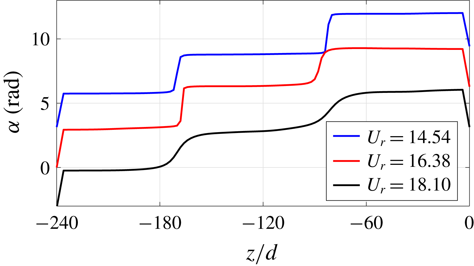
Figure 10 presents the amplitude, phase response, and $C_{lv}$ distribution along the flexible model at $U_{r}=14.54$ of the modal group ‘ $5/3$ ’, $U_{r}=16.38$ of the modal group ‘ $6/3$ ’ and $U_{r}=18.1$ of the modal group ‘ $6/3$ ’. For all three values of $U_{r}$ , the cylinder responds in the 3rd mode in the CF direction. With increasing $U_{r}$ , the distribution of the CF displacement changes from a small and symmetric response to an asymmetric response with a prominent peak. In figure 11, we plot the relative phase $\unicode[STIX]{x1D6FC}$ of the oscillation at different locations along the flexible model span in the CF direction. The relative phase $\unicode[STIX]{x1D6FC}$ is defined as zero at $z/d=-240$ and as the angle of the oscillation at each location. Comparing the blue line of $U_{r}=14.54$ and the black line of $U_{r}=18.1$ in figure 11, as the CF response changes from symmetric to asymmetric, the $\unicode[STIX]{x1D6FC}$ distribution has a smoother transition at the CF node, which indicates a stronger mixture of travelling and standing wave responses (Bourguet et al. Reference Bourguet, Karniadakis and Triantafyllou2013).

Comparing the amplitude response with the $C_{lv}$ distribution, four interesting points can be raised. First, in general the rigid cylinder database can capture the distribution of $C_{lv}$ along the model. Second, the $\unicode[STIX]{x1D703}$ values corresponding to the CCW trajectory are associated with the positive energy-in from the fluid to the structure. Third, when the CF amplitude is smaller, the $C_{lv}$ distribution also obtains a smaller amplitude both positively and negatively, shown in the comparison between $U_{r}=14.54$ and $U_{r}=16.38$ (see figure 10). Last, for the asymmetric CF response with a mixture of standing and travelling wave patterns, $C_{lv}$ is also found asymmetrically distributed along the flexible model, with the region of large negative values associated with the large CF amplitude, shown in figure 10(f) at $U_{r}=18.1$ .

Figure 11.

Relative phase $\unicode[STIX]{x1D6FC}$ of the CF vibration at different locations along the span of the flexible model for blue, $U_{r}=14.54$ ; red, $U_{r}=16.38$ ; black, $U_{r}=18.1$ . For visual clarity, we assign an offset for blue and black curves.

From the samples of $C_{lv}$ measured via the rigid cylinder forced vibration in appendix D, we find that $\unicode[STIX]{x1D703}$ corresponding to the CCW motion are associated with the positive $C_{lv}$ when $A_{y}/d$ is small, while $C_{lv}$ is largely negative for clockwise motion. In addition, $C_{lv}$ decreases with increasing $A_{y}/d$ and $A_{x}/d$ . In the experiment, when the flexible cylinder vibrates at the onset of the 3rd mode in the CF direction at $U_{r}=14.54$ , the amplitude response is small, as the true reduced frequency of the vibration is large and far away from the Strouhal frequency. It is similar to the low mass ratio rigid cylinder free vibration at the start of the initial branch with a large reduced frequency corresponding to small CF amplitudes (Jauvtis & Williamson Reference Jauvtis and Williamson2003). With the increase of $U_{r}$ , the true reduced frequency of the flexible cylinder decreases and gets close to the Strouhal frequency, so the fluid and structure coupling effect becomes stronger. This results in a larger CF amplitude associated with a stronger energy exchange between the fluid and the structure in the CF direction. Therefore, comparing $U_{r}=16.38$ to $U_{r}=14.54$ , shown in figures 10(b) and 10(d), we see a larger magnitude for both negative and positive $C_{lv}$ distribution along the model span. Further increasing $U_{r}$ , the CF amplitude tends to get larger, and if the CF amplitude remains symmetric and hence increases altogether along the span, more energy is required from the fluid to the structure, as the structure dissipates more energy via damping over one vibration cycle. However, in general, $C_{lv}$ decreases with increasing $A_{y}/d$ (such a trend can be seen in figure 27 in appendix B of the rigid cylinder forced vibration) and therefore the energy balance between the fluid and the structure cannot be maintained. Subsequently, due to the alternative clockwise (CW) and CCW $\unicode[STIX]{x1D703}$ distribution along the flexible model, the asymmetric response in the CF direction is allowed to grow. A large amount of fluid energy transfers into the flexible model in its small $A_{y}/d$ and CCW $\unicode[STIX]{x1D703}$ region, and then transmits inside the flexible model, which leads to the appearance of a stable travelling wave. Due to the finite length of the model, a standing wave response with a large amplitude forms close to the boundary due to the reflection, and the ambient fluid helps the structure to dissipate energy at that region with a large CF amplitude.

3.4 Modal group switch and added mass variation in and between modal groups

In the previous sections we showed that the sectional hydrodynamic coefficients for a flexible cylinder are predicted accurately by the forced vibration experiment on rigid cylinders. In this section, we focus on understanding why the added mass coefficient in the CF direction undergoes such large variations and why it is different for different modal groups.

The spatial mean added mass coefficient $\overline{C_{m}}$ in either the IL or the CF direction for the flexible cylinder is calculated for all $U_{r}$ based on the following equation:

(3.1) $$\begin{eqnarray}\overline{C_{m}}=\frac{1}{L}\int _{0}^{L}C_{m}(z)\,\text{d}z.\end{eqnarray}$$

The reconstructed $\overline{C_{m}}$ from the motion data and the corresponding predicted values from the rigid cylinder experiments are plotted together against $U_{r}$ in figure 12 for $\overline{C_{my}}$ and figure 13 for $\overline{C_{mx}}$ . Both figures show good agreement between the flexible cylinder measurements and the rigid cylinder prediction. We obtained that the averaged relative difference of $\overline{C_{my}}$ between the measurement of the flexible cylinder ( $250\leqslant Re\leqslant 2\,300$ ) and the prediction of the rigid cylinder forced vibration ( $Re=5\,715$ ), namely $(|\overline{C_{my}^{rigid}}-\overline{C_{my}^{flex}}|)/|\overline{C_{my}^{flex}}|$ , is around 17.4 %. The $\overline{C_{my}}$ exhibits different behaviour in the modal group ‘ $2n:n$ ’ (highlighted in figures 12 and 13 with a shaded region) and the modal group ‘ $2n-1:n$ ’. Values of $\overline{C_{my}}$ in the modal group ‘ $2n:n$ ’ are close to 0.5, which drives the natural frequency of the flexible model to larger values than the predicted $n$ th modal frequency in still water, assuming $C_{m}=1.0$ . In contrast, $\overline{C_{my}}$ in the modal group ‘ $2n-1:n$ ’ is larger than 1.0 (the black dashed line denotes $\overline{C_{my}}=1.0$ in figure 12). The predicted true modal frequencies $f_{nx}^{true}$ and $f_{ny}^{true}$ for the IL and the CF vibrations are given by equation (3.2) as follows:

(3.2) $$\begin{eqnarray}\left.\begin{array}{@{}c@{}}\displaystyle f_{ny}^{true}\simeq \overline{f_{ny}^{true}}=\frac{n}{2L}\sqrt{\frac{\overline{T}}{(\unicode[STIX]{x1D707}+\overline{\unicode[STIX]{x1D707}_{y}})}},\\ \displaystyle f_{nx}^{true}\simeq \overline{f_{nx}^{true}}=\frac{m}{2L}\sqrt{\frac{\overline{T}}{(\unicode[STIX]{x1D707}+\overline{\unicode[STIX]{x1D707}_{x}})}},\end{array}\right\}\end{eqnarray}$$

where $\overline{\unicode[STIX]{x1D707}_{y}}=\overline{C_{my}}\unicode[STIX]{x1D70C}(\unicode[STIX]{x03C0}/4)D^{2}$ is the spatial mean added mass per unit length in the CF direction, $\overline{\unicode[STIX]{x1D707}_{x}}=\overline{C_{mx}}\unicode[STIX]{x1D70C}(\unicode[STIX]{x03C0}/4)D^{2}$ is the spatial mean added mass per unit length in the IL direction and $\overline{T}$ is the average tension along the model. The difference between $f_{n}^{true}$ and $\overline{f_{n}^{true}}$ is addressed in appendix C. In the current experiment, $\overline{C_{my}}$ shows a large variation between different modal groups, while $\overline{C_{mx}}$ does not vary much and stays close to 0.5, as shown in figure 13.

Figure 12.

Spatial mean added mass coefficient in the CF direction $\overline{C_{my}}$ as a function of $U_{r}$ . Here $\overline{C_{my}}>1.0$ corresponds to the modal group ‘ $2n-1:n$ ’ and $\overline{C_{my}}<1.0$ corresponds to the modal group ‘ $2n:n$ ’. The shaded area highlights the modal group ‘ $2n:n$ ’.

Figure 13.

Spatial mean added mass coefficient in the IL direction $\overline{C_{mx}}$ as a function of $U_{r}$ . Unlike $\overline{C_{my}}$ , $\overline{C_{mx}}<1.0$ for all modal groups. The shaded area highlights the modal group ‘ $2n:n$ ’.

As pointed out in Dahl et al. (Reference Dahl, Hover, Triantafyllou and Oakley2010), the effective IL and CF added mass coefficients vary collaboratively in order to reach a true natural frequency ratio of $f_{nx}^{true}/f_{ny}^{true}=2.0$ , and a dual resonance of stable oscillations in both the IL and the CF directions can be achieved. For the uniform flexible cylinder VIV, the same criterion should be held for the fluid added mass, as the system’s true natural frequency has to be altered in order to match the external frequency. It is shown in equation (3.3) that the system’s true natural frequency, the system vibration frequency and the external disturbance frequency, namely the shedding vortex frequency should coincide with each other, i.e.

(3.3) $$\begin{eqnarray}\left.\begin{array}{@{}c@{}}f_{y}=f_{ny}^{true},\quad f_{x}=f_{nx}^{true},\\ f_{x}=2f_{y}=2f_{v},\end{array}\right\}\end{eqnarray}$$

where $f_{x}$ and $f_{y}$ are the vibration frequencies of the flexible cylinder in the IL and the CF directions, respectively, $f_{nx}^{true}$ and $f_{ny}^{true}$ are the true natural frequencies of the flexible cylinder in the IL and the CF directions and $f_{v}$ is the vortex shedding frequency in the cylinder wake. When $m=2n$ , the added mass coefficient in the IL and the CF directions is given by the following equation, based on equations (3.2) and (3.3),

(3.4) $$\begin{eqnarray}\overline{C_{my}}\simeq \overline{C_{mx}}.\end{eqnarray}$$

When $m=2n-1$ , we also derived the following equation for the added mass coefficient in the IL and the CF directions,

(3.5) $$\begin{eqnarray}\overline{C_{my}}\simeq \frac{4n^{2}-(2n-1)^{2}}{(2n-1)^{2}}m^{\ast }+\frac{4n^{2}}{(2n-1)^{2}}\overline{C_{mx}}.\end{eqnarray}$$

In figure 12, we plot the predicted $\overline{C_{my}}$ (black line) based on the $\overline{C_{mx}}$ in figure 13 (blue line). Equations (3.4) and (3.5) give a large variation of the $\overline{C_{my}}$ between different modal groups from a relatively constant $\overline{C_{mx}}$ over $U_{r}$ .

Next we focus on $U_{r}=10.75$ of the modal group ‘ $4/2$ ’, $U_{r}=12.66$ of the modal group ‘ $4/2$ ’ and $U_{r}=13.61$ of the modal group ‘ $5/3$ ’ in order to explain how the added mass changes when $U_{r}$ increases in and between modal groups.

Figures 14 and 15 present the $C_{my}$ and $C_{mx}$ predictions as a function of $V_{r}$ and $\unicode[STIX]{x1D703}$ from the forced oscillating rigid cylinder with matched $A_{x}/d$ and $A_{y}/d$ at different locations along the flexible cylinder at $U_{r}=10.75$ , $U_{r}=12.66$ and $U_{r}=13.61$ . A detailed description of the added mass coefficient in both the IL and CF directions with respect to $V_{r}$ and $\unicode[STIX]{x1D703}$ is presented in appendix D. The grey transparent slices highlight the true reduced velocity $V_{r}$ and the solid black line denotes the $\unicode[STIX]{x1D703}$ distribution. The intersection between the $C_{my}$ and $C_{mx}$ contour and the $\unicode[STIX]{x1D703}$ line is highlighted with the yellow diamond, denoting the predicted sectional $C_{my}$ and $C_{mx}$ of the flexible model via the rigid cylinder hydrodynamic database with the same values of $A_{y}/d$ , $A_{x}/d$ , $V_{r}$ and $\unicode[STIX]{x1D703}$ .

Figure 14.

The $C_{my}$ values along the span of the flexible model interpolated from the rigid cylinder forced vibration experiments. The colour contours of $C_{my}$ are computed as a function of $V_{r}$ and $\unicode[STIX]{x1D703}$ from the forced oscillating rigid cylinder with the matched $A_{x}/d$ and $A_{y}/d$ . The $\unicode[STIX]{x1D703}$ distribution (the solid black line) and $V_{r}$ (the shaded plane) highlight the $C_{my}$ value at each contour plane (the yellow diamond).

Figure 15.

The $C_{mx}$ values along the span of the flexible model interpolated from the rigid cylinder forced vibration experiments. The colour contours of $C_{mx}$ are computed as a function of $V_{r}$ and $\unicode[STIX]{x1D703}$ from the forced oscillating rigid cylinder with the matched $A_{x}/d$ and $A_{y}/d$ . The $\unicode[STIX]{x1D703}$ distribution (the solid black line) and $V_{r}$ (the shaded plane) highlight the $C_{my}$ value at each contour plane (the yellow diamond).

The flexible cylinder in uniform flow vibrates at the same frequency along the entire model, resulting in the same $V_{r}$ at each location. The $\unicode[STIX]{x1D703}$ distribution has a $\unicode[STIX]{x03C0}$ phase jump at the IL node. As shown from the rigid cylinder forced vibration experiment (appendix B), $\unicode[STIX]{x1D703}$ has a strong influence on $C_{my}$ , and therefore $C_{my}$ changes drastically at the IL node along the flexible cylinder. Furthermore, the effect of $A_{x}/d$ and $A_{y}/d$ on $C_{my}$ is weak, so inside a half-wavelength of the IL response mode, $C_{my}$ keeps a relatively constant value, which results in a stepped distribution of $C_{my}$ , as shown in figure 14. In addition, similar to $C_{my}$ , $C_{mx}$ also distributes along the model in a stepped fashion, but compared to the large variation of $C_{my}$ distribution, $C_{mx}$ changes slightly, as shown in figure 15.

Here we give more details on what happens to the fluid added mass distribution with an increasing $U_{r}$ , and explain why the flexible cylinder switches modal group. To begin with, as $U_{r}$ increases from 10.75 to 13.61 (correspondingly, the towing velocity changes from $0.11~\text{m}~\text{s}^{-1}$ to $0.14~\text{m}~\text{s}^{-1}$ ), the vortex shedding frequency tends to increase. In order to maintain a stable flexible cylinder VIV in the lock-in region, for the CF vibrations, the three frequencies have to be the same: $f_{y}$ , $f_{v}$ and $f_{ny}^{true}$ , shown in equations (3.2) and equations (3.3). In each experiment, the mean tension $T$ , length $L$ and structural mass per unit length $\unicode[STIX]{x1D707}$ of the model are fixed, and only the mode number $n$ and the spatial average fluid added mass per unit length $\overline{\unicode[STIX]{x1D707}}$ can be altered to change the structural natural frequency.

Figures 14(a) and 14(b) shows that with the increase of $U_{r}$ from 10.75 to 12.66, the flexible model still remains in the same modal group, but in order to match $f_{ny}^{true}$ and the increasing $f_{v}$ , the $V_{r}$ and $\unicode[STIX]{x1D703}$ distribution are adjusted to find a proper combination of the fluid added mass distribution. Comparing figure 14(b) at $U_{r}=12.66$ to figure 14(a) at $U_{r}=10.75$ , the sectional $C_{my}$ at some locations along the model approaches its negative minimum, predicted by the rigid cylinder forced vibration experiment. Further increasing $U_{r}$ (the towing velocity increases in the experiment), if the flexible model is in the same modal group, a smaller $\overline{\unicode[STIX]{x1D707}_{y}}$ is required in order to increase $f_{ny}^{true}$ for higher  $f_{v}$ . However, no corresponding $V_{r}$ and $\unicode[STIX]{x1D703}$ distribution can be found, as at smaller $U_{r}$ , $C_{my}$ at different locations along the flexible model has already reached or is close to the negative minimum. Note here that not only the fluid added mass has to be adjusted to agree with equations (3.2) and (3.3), but also the net energy between the structure and the fluid should be balanced, and hence there are also constraints on $C_{lv}$ and $C_{dv}$ .

With no possibility of finding a proper added mass distribution to keep the same modal response in the CF direction, the mode number of the flexible model vibration needs to switch. Comparing figure 14(c) at $U_{r}=13.61$ to figure 14(b) at $U_{r}=12.66$ , the flexible model switches from the modal group ‘ $4/2$ ’ to the modal group ‘ $5/3$ ’. With such mode number switch, the structure natural frequency experiences a big jump – for example, it jumps from $2f_{n1}$ for $U_{r}=12.66$ to $3f_{n1}$ for $U_{r}=13.61$ in the CF direction. However, the vortex shedding frequency increases slightly due to a small increase of $U_{r}$ , so the $\unicode[STIX]{x1D703}$ distribution and the $V_{r}$ value of the flexible model have to adjust accordingly, as shown in figure 14.

4.1 Three-dimensional wake structure behind the flexible cylinder: distortion of shed vortices at IL nodes

Figure 18.

Linking the structural response (a–d) with the wake patterns (e). The simulation results show the dislocation of the shed vortex tubes around IL nodes at $U_{r}=14.54$ , highlighting the ‘2S’ mode both above and below the black dashed line: (a) the IL and the CF amplitude response; (b) the PSD of the CF displacement; (c) the PSD of the CF flow velocity; (d) phase difference $\unicode[STIX]{x1D6FC}$ of the CF flow velocity; (e) a series of snapshots of the vortex shedding over one period at $t=0$ , $t=\frac{1}{4}T$ , $t=\frac{1}{2}T$ , $t=\frac{3}{4}T$ and $t=T$ from left to right, where $T$ is the vibration period at $U_{r}=14.54$ . The black dashed line marks location $z/d=-48$ . Note that the CF flow velocity is taken at three diameters downstream from the mean IL displacement and the vortices are represented by isosurfaces of $Q=0.1$ and coloured by $\unicode[STIX]{x1D714}_{z}$ .

Figure 19.

Linking the structural response (a–d) with the wake patterns (e). The simulation results show the dislocation of the shed vortex tubes around IL nodes at $U_{r}=17.22$ , highlighting the ‘2S’ mode above the black dashed line and the ‘P $+$ S’ mode below the black dashed line: (a) the IL and the CF amplitude response; (b) the PSD of the CF displacement; (c) the PSD of the CF flow velocity; (d) phase difference $\unicode[STIX]{x1D6FC}$ of the CF flow velocity; (e) a series of snapshots of the vortex shedding over one period at $t=0$ , $t=\frac{1}{4}T$ , $t=\frac{1}{2}T$ , $t=\frac{3}{4}T$ and $t=T$ from left to right, where $T$ is the vibration period at $U_{r}=17.22$ . The black dashed line marks location $z/d=-200$ . Note that the CF flow velocity is taken at three diameters downstream from the mean IL displacement and the vortices are represented by isosurfaces of $Q=0.1$ and coloured by $\unicode[STIX]{x1D714}_{z}$ .

In order to assess the spanwise correlation of the wake structure behind the flexible model, a frequency and phase analysis is applied to the cross-flow component of the flow velocity, located at three diameters downstream from the mean IL displacement.

Figures 18 and 19, each presents the PSD (subfigure c) and the phase distribution (subfigure d) of the cross-flow component of the flow velocity at $U_{r}=14.54$ and $U_{r}=17.22$ , together with the IL and the CF amplitude response (subfigure a) and the PSD of the CF displacement (subfigure b). Comparing subfigures (b) and (c) from figures 18 and 19, it is shown that the ‘lock-in’ happens along the entire model span, as the CF vibration frequency is equal to the vortex shedding frequency everywhere. However, the phase analysis on the cross-flow velocity component reveals that at IL nodes the phase of the flow velocity changes drastically, whereas it keeps a relatively constant value along the half-wavelength between two adjacent IL nodes. At IL nodes, the phase $\unicode[STIX]{x1D703}$ between the IL and CF trajectory undergoes a phase jump by $\unicode[STIX]{x03C0}$ , which leads to a change in the vortical structures, as reflected in the snapshots of the local vortex shedding around IL nodes over one vibration cycle in figure 18(e) at $U_{r}=14.54$ and in figure 19(e) at $U_{r}=17.22$ . We can see that there is a shift of the vortex tubes (positive vortex in yellow) in space as well as a vortex pattern switch above and below the black dash line denoting one of the IL nodes along the flexible model.

Specifically, at $U_{r}=17.22$ , along the span of the cylinder, the vortices shed in cells that are separated by the IL nodes, and the relative motion between the local cylinder oscillation and vortex formation also breaks into the same cells, which explains the variation of the added mass along the flexible model span, shown in figure 17(c). At $U_{r}=14.54$ , the response is a modal group ‘ $5/3$ ’ (model group type ‘ $2n-1/n$ ’), but unlike case of $U_{r}=17.22$ , here the IL and CF nodes do not coincide with each other. As shown in figure 18, apart from the dislocation of the vortex tube around $z/d=-50$ , $z/d=-94$ , $z/d=-146$ and $z/d=-189$ where IL nodes reside in, an interesting phenomenon called the ‘void’ vortex shedding region could be observed at $z/L=-82$ and $z/L=-158$ , both of which are CF nodes. A similar phenomenon has been reported experimentally by Gilbert & Sigurdson (Reference Gilbert and Sigurdson2010) and Bangash & Huera-Huarte (Reference Bangash and Huera-Huarte2015). However, note that in the previous experiments, the ‘void’ regions appear at IL node and CF anti-node, which is different from the current simulation results. The difference may be due to different $Re$ , vibration mode number and, perhaps more importantly, the IL vibration amplitude. Unlike the current simulation, the IL amplitude is much smaller than the CF amplitude in the aforementioned two experiments. The ‘void’ vortex shedding region is accompanied with the local vortex pattern change, e.g. an attached symmetric non-shedding vortex pair behind the cylinder as reported by Bangash & Huera-Huarte (Reference Bangash and Huera-Huarte2015), which leads to a large local variation of $C_{my}$ , shown in figure 18 of $z/d=-70$ to $z/d=-90$ and $z/d=-150$ to $z/d=-170$ .

4.2 Cross-sectional 2-D wake pattern: CF motion versus local vortex shedding

As pointed out by Sarpkaya (Reference Sarpkaya2004), in flexibly mounted rigid cylinder experiments, a slight change of the relative motion between the cylinder oscillation and vortex formation can alter the hydrodynamic coefficients and the VIV response significantly. In this section, we use the 2-D snapshots of the spanwise field around the oscillating cylinder to explain the noted changes in the hydrodynamic coefficients.

Figure 20.

Simulation results of 2-D snapshots of the vortices at  $z/d=-185$ for $U_{r}=17.22$ over one period of CF oscillation: (a–e) instantaneous field of $\unicode[STIX]{x1D714}_{z}$ ; (f) time trace of the cylinder CF motion (a–c) and the oscillating lift force (d–f). The red circle highlights the corresponding time from (a) to (e).

Figure 21.

Simulation results of 2-D snapshots of the vortices at  $z/d=-210$ for $U_{r}=17.22$ over one period of CF oscillation: (a–e) instantaneous field of $\unicode[STIX]{x1D714}_{z}$ ; (f) time trace of the cylinder CF motion (a–c) and the oscillating lift force (d–f). The red circle highlights the corresponding time from (a) to (e).

Figures 20 to 23 provide five consecutive 2-D snapshots of the $\unicode[STIX]{x1D714}_{z}$ field around the flexible cylinder at a given location for $U_{r}=14.54$ and $U_{r}=17.22$ over one period of the CF vibration. In subfigures (f), we plot the time trace of the cylinder CF motion (black) as well as the lift coefficient (blue) at the corresponding location, with the red circles denoting the time of the snapshots. At $z/d=-210$ for $U_{r}=17.22$ in figure 20, $C_{my}$ is a small negative value, as the subfigures (f) show that the fluctuating lift force of a small amplitude is in-phase with the acceleration. Subfigures (a) to (e) display a flow pattern as follows: at the bottom of the cylinder trajectory (subfigures a), one CCW vortex is about to detach from the cylinder rear, while a CW vortex forms in the upper shear layer. In subfigures (b), as the cylinder moves upwards, the CW vortex extends across the cylinder rear and pairs with the rolled-up CCW vortex in the wake. In subfigures (c), the cylinder then moves to the top of its oscillation where the CW vortex is stretched to split into two CW vortices. When the cylinder moves downwards in the second half-cycle of the oscillation (subfigures d), one of the two CW vortices moves together with the previously shed positive vortex, resulting in a vortex pair detaching from the cylinder in the lower half of the wake. In the meantime, the other CW vortex rolls up and is ready to detach from the cylinder in the upper half of the wake. This results in a shedding mode of ‘P $+$ S’ (Williamson & Govardhan Reference Williamson and Govardhan2008). Meanwhile, at $z/d=-185$ for $U_{r}=17.22$ in figure 21, $C_{my}$ exhibits a large positive value, as the subfigures (f) show that the fluctuating lift force of a large amplitude is in anti-phase with acceleration. Subfigures (a) to (e) display a different flow pattern of a classical ‘2S’ mode, compared to the ‘P $+$ S’ mode found in the CW $C_{my}$ region, as follows: at the bottom of the cylinder trajectory (subfigures a), one CW vortex is about to leave the cylinder in the upper half of the wake, while a CCW vortex forms on the upper half of the cylinder rear. In subfigures (b), as the cylinder moves upwards, the upper negative shear layer grows at the cylinder back and, in the meantime, the CCW vortex rolls up and is ready to detach. In subfigures (c), the cylinder then moves to its top of the oscillation where the CCW vortex moves downstream in the lower half of the wake. When the cylinder moves downwards in the second half-cycle of the oscillation (subfigures d), another CW vortex grows in strength in the upper half of the wake and then the whole process repeats from subfigures (a).

Comparing the vortex formation around the oscillating cylinder between the regions of $C_{my}<0$ and $C_{my}>0$ , a clear difference can be seen in the timing of the vortex formation relative to the cylinder motion. Furthermore, it is found that for the positive $C_{my}$ region with the ‘2S’ mode, the shedding vortex forms close to the moving cylinder, compared to the negative $C_{my}$ region with the ‘P $+$ S’ mode, which is also observed in the CF-only rigid cylinder vibration of controlled trajectory by Carberry et al. (Reference Carberry, Sheridan and Rockwell2005). Nonetheless, in order to thoroughly understand the coupling mechanism between the vortex shedding and cylinder vibration, more simulations and experiments of the rigid cylinder vibrating with controlled in-line and cross-flow coupled trajectories are needed, as well as more studies of the effect of the in-line motion on the forces and the wake patterns.

Figure 22.

Simulation results of 2-D snapshots of the vortices at  $z/d=-90$ for $U_{r}=14.54$ over one period of CF oscillation: (a–e) instantaneous field of $\unicode[STIX]{x1D714}_{z}$ ; (f) time trace of the cylinder CF motion (a–c) and the oscillating lift force (d–f). The red circle highlights the corresponding time from (a) to (e).

Figure 23.

Simulation results of 2-D snapshots of the vortices at  $z/d=-145$ for $U_{r}=14.54$ over one period of CF oscillation: (a–e) instantaneous field of $\unicode[STIX]{x1D714}_{z}$ ; (f) time trace of the cylinder CF motion (a–c) and the oscillating lift force (d–f). The red circle highlights the corresponding time from (a) to (e).

Furthermore, at $z/d=-90$ and $z/d=-145$ for $U_{r}=14.54$ of the model group ‘ $5/3$ ’ figures 22(a–e) and 23(a–e) display a flow pattern of the classical ‘2S’ mode, similar to the flow pattern in the region of large positive $C_{my}$ for $U_{r}=17.22$ . However, at $U_{r}=14.54$ , the vortices no longer form at the upper- or lower-half side of the cylinder, instead they appear directly at the rear of the cylinder, close to the centre line of the cylinder CF oscillation. As a result, the cylinder wake is narrower with the cores of the alternating CCW and CW vortices aligned with the centre line of the cylinder CF motion. In contrast, in figure 20 of ‘2S’ vortex mode, CCW and CW vortices distinctively occupy the upper- and lower-half of the wake, which leads to a wider wake.