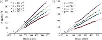
1. Introduction
Velocimetry techniques based on total internal reflection fluorescence (TIRF) have enlightened our understanding of the behaviour of Newtonian flows and particles near boundaries. The method was pioneered by Yoda (Zettner & Yoda Reference Zettner and Yoda2003; Sadr et al.
Reference Sadr, Yoda, Zheng and Conlisk2004; Sadr, Li & Yoda Reference Sadr, Li and Yoda2005; Li, Sadr & Yoda Reference Li, Sadr and Yoda2006; Sadr et al.
Reference Sadr, Hohenegger, Li, Mucha and Yoda2007; Li & Yoda Reference Li and Yoda2008, Reference Li and Yoda2010) and Breuer (Jin et al.
Reference Jin, Huang, Park, Yoo and Breuer2004; Guasto, Huang & Breuer Reference Guasto, Huang and Breuer2006; Huang, Guasto & Breuer Reference Huang, Guasto and Breuer2006; Huang & Breuer Reference Huang and Breuer2007; Guasto & Breuer Reference Guasto and Breuer2009; Huang, Guasto & Breuer Reference Huang, Guasto and Breuer2009), and further developed or used by several authors (Bouzigues, Tabeling & Bocquet Reference Bouzigues, Tabeling and Bocquet2008; Kazoe et al.
Reference Kazoe, Iseki, Mawatari and Kitamori2013). It consists of seeding the fluid with fluorescent nanoparticles and operate in an evanescent field near a wall/liquid interface. In such conditions, the fluorescent particles emit a light whose intensity is expected to decrease exponentially with their altitudes (i.e. their distances to the wall) and it becomes envisageable, by translating intensities into distances, to determine the location of each of them with respect to the wall without being subjected to diffraction limit. With the cameras available today on the market, the theoretical spatial precision on the determination of the altitudes obtained with this technique is subnanometric, but in practice, for a number of reasons that will be explained later, the best altitude accuracy reported thus far in the literature is 30 nm (Li & Yoda Reference Li and Yoda2010). Still this represents an improvement by more than one order of magnitude in comparison with well-resolved techniques such as
 ${\it\mu}$
PIV (micro particle image velocimetry) (Santiago et al.
Reference Santiago, Wereley, Meinhart, Beebe and Adrian1998; Meinhart, Wereley & Santiago Reference Meinhart, Wereley and Santiago1999; Tretheway & Meinhart Reference Tretheway and Meinhart2002; Joseph & Tabeling Reference Joseph and Tabeling2005; Zheng, Kong & Silber-Li Reference Zheng, Kong and Silber-Li2013).
Measuring velocity, diffusion constant, speed distributions, etc.at various locations determined with a nanometric accuracy would be a breakthrough for flow instrumentation. It would open the possibility to analyse nanoflows in a great variety of contexts (Mijatovic, Eijkel & van den Berg Reference Mijatovic, Eijkel and van den Berg2005; Hu & Li Reference Hu and Li2007; Sparreboom, van den Berg & Eijkel Reference Sparreboom, van den Berg and Eijkel2009). Examples concern lubricating films in concentrated emulsions and foams (Kimura & Okada Reference Kimura and Okada1989; Schmid & Wilson Reference Schmid and Wilson1995; Briceño & Joseph Reference Briceño and Joseph2003), depleted layers in polymer solutions (De Gennes Reference De Gennes1981; Vincent Reference Vincent1990), grain dynamics in microgel concentrated suspensions (Meeker, Bonnecaze & Cloitre Reference Meeker, Bonnecaze and Cloitre2004; Sessoms et al. Reference Sessoms, Bischofberger, Cipelletti and Trappe2009), Debye layers (Bouzigues et al. Reference Bouzigues, Tabeling and Bocquet2008), grafted brush structure (de Gennes Reference de Gennes1980; Murat & Grest Reference Murat and Grest1989) and polymer melt near-wall behaviour (Brochard & De Gennes Reference Brochard and De Gennes1992; Brazhnik, Freed & Tang Reference Brazhnik, Freed and Tang1994, etc.). TIRF-based velocimetry has thereby the potential to open new interesting avenues in fluid dynamics research.
Nonetheless, TIRF-based velocimetry suffers from a number of limitations and artefacts that have been analysed by a number of investigators (Choi, Westin & Breuer Reference Choi, Westin and Breuer2003; Sadr et al. Reference Sadr, Li and Yoda2005, Reference Sadr, Hohenegger, Li, Mucha and Yoda2007; Huang et al. Reference Huang, Guasto and Breuer2006; Huang & Breuer Reference Huang and Breuer2007; Li & Yoda Reference Li and Yoda2010). The main problems are as follows.
-
(i) Brownian wandering. Nanoparticles are subjected to Brownian motion while the exposure times, or the delay times between two successive captures are limited by the performances of the camera. During the exposure time
 ${\it\tau}$
(typically, 1 or 2 ms) particles explore a region equal
$\sqrt{2D{\it\tau}}$
, in which
$D$
is the diffusion coefficient of the particle in the fluid. Using an Einstein estimate of the diffusion constant, one finds that there is an optimal scale
$l_{opt}$
, defined by (1.1)for which particle radius equals to Brownian standard-type deviation (here,
$$\begin{eqnarray}l_{opt}=\left(\frac{kT{\it\tau}}{3{\rm\pi}{\it\mu}}\right)^{1/3}\end{eqnarray}$$
$k$
is the Boltzmann constant,
$T$
the absolute temperature and
${\it\mu}$
the fluid viscosity). Particles much smaller than
$l_{opt}$
develop large Brownian excursions and therefore probe large volumes. Particles larger than
$l_{opt}$
also degrade the resolution because of their size. Therefore, expression (1.1) provides a reference scale for establishing the spatial resolution that TIRF-based velocimetry can achieve. It turns out that the best precision on the particle altitude measurement achieved today (30 nm) coincides, in terms of order of magnitude, with
$l_{opt}$
. In the future, progress on the spatial resolution of TIRF-based velocimetry will obviously be facilitated by progress in camera technology, but today the possibility of improving the situation with the existing cameras is worth being considered.
-
(ii) Biases induced by the heterogeneities of the spatial distribution of the particles. The distribution of particles is not homogeneous in space, which generates difficulties in the establishment of the relationship between the particle trajectories and the fluid speed. In aqueous solutions, and in typical situations, the colloidal particles seeding the flow are negatively charged and the wall develops negative surface charges. A Debye layer builds up, repelling the colloids and thus depleting the near wall region in particles (Oberholzer, Wagner & Lenhoff Reference Oberholzer, Wagner and Lenhoff1997). Dielectrophoretic effects, pointed out recently by Yoda (Cevheri & Yoda Reference Cevheri and Yoda2014) may also contribute to shape the heterogeneity field. Other sources of inhomogeneities in the spatial distributions of the particles are diffusion gradients, inducing a drift oriented away from the wall, and closer to the walls, short-range forces (Koch Reference Koch1989). Since all measurements involve spatial averaging, either for statistical reasons or because of Brownian wandering, the interpretation of the averages obtained with such heterogeneities is delicate (particles spatial distributions weight the functions that are spatially averaged). In the present state of the art, Yoda (Li et al. Reference Li, Sadr and Yoda2006; Li & Yoda Reference Li and Yoda2010) partitioned the space into three regions, assuming homogeneity in each of them. The velocity profiles obtained with this approach, being composed, for reasons linked to Brownian motion, of only three points in the 200–500 nm range (Li & Yoda Reference Li and Yoda2010), are modestly resolved. One question is whether it is possible to improve the situation, for instance by reducing the size of the intervals over which averages are determined, while ensuring acceptable statistical convergence and controlling or reducing statistical biases.
-
(iii) Polydispersity of the particle characteristics. The particles currently used in the TIRF velocimetry experiments have polydispersivities in size, quantum efficiency and numbers of incorporated fluorophores. Since the determination of the position relies on intensity measurements, this variability impacts the accuracy at which the particles can be localized. In practice, using 100–200 nm fluorescent particles, for which polydispersivity lies between 5 % and 10 % is acceptable, while using 20 nm, with polydispersitivities between 20 % and 30 % is problematic.
-
(iv) Position of the wall. Determining the wall location accurately is critical, since errors made at this level impact directly the accuracy of the slip length determination. Determining the wall location necessitates separate measurements that must be made in situ, in order to keep the flow geometry and the instrumentation environment unchanged. One of the techniques consists in enhancing adsorption by adding salt (and then suppressing electrical screening), and measuring the intensity distribution of the particles adsorbed onto the wall (Li & Yoda Reference Li and Yoda2010). In the present state of the art, these measurements are subjected to significant uncertainties, due, mostly, to an inaccurate analysis of the bleaching process.
-
(v) Relating particle speeds to flow speeds. Even though the particle positions and speeds were accurately determined, the information would be not sufficient for determining the flow. Close to a wall, owing to various phenomena well documented in the literature (hindered diffusion, slowing down, etc.) the particle speed is not equal to the flow speed. Models must therefore be developed to convert particle speed data into flow speed data.


Today, TIRF velocimetry has enlightened our understanding of the behaviour of Newtonian fluids close to a wall by establishing the structure of the velocity profiles and investigating how particles are transported. However, the biases and artefacts discussed above severely affect its capability to discuss slippage phenomena. The quantity characterizing slippage is the slip length, i.e. for TIRF-based velocimetry, the length obtained by extrapolating the velocity profiles down to zero (thus, the ‘extrapolated slip length’). Slip length measurements have attracted the interest of a community for more than one decade and it is now well documented for the case of Newtonian fluids (Bocquet & Barrat Reference Bocquet and Barrat2007; Bocquet & Charlaix Reference Bocquet and Charlaix2010). Slip lengths can be taken to benchmark different techniques. At the moment, the best accuracy (based on standard-type deviation) obtained on the slip length measurements by TIRF is
 $\pm 30~\text{nm}$
(Huang et al.
Reference Huang, Guasto and Breuer2006; Li & Yoda Reference Li and Yoda2010). This limited accuracy ranks TIRF velocimetry well below surface force apparatus (SFA) (SFA; Cottin-Bizonne et al.
Reference Cottin-Bizonne, Cross, Steinberger and Charlaix2005), which currently achieves
 $\pm 2~\text{nm}$
, and other methods, such as pressure drop measurements (Choi et al.
Reference Choi, Westin and Breuer2003) which achieves
 $\pm 5~\text{nm}$
, fluorescence correlation spectroscopy (FCS) which has 5 nm of accuracy (Joly, Ybert & Bocquet Reference Joly, Ybert and Bocquet2006), and double-focus fluorescence cross-correlation, which attains of 10 nm accuracy (Vinogradova et al.
Reference Vinogradova, Koynov, Best and Feuillebois2009). Worse, the actual TIRF-based slippage measurements do not allow to distinguish between hydrophilic and hydrophobic surfaces (Li & Yoda Reference Li and Yoda2010); in another work (Huang et al.
Reference Huang, Guasto and Breuer2006) slip lengths lying between 26 and 57 nm are found for hydrophilic surfaces, which disagrees with the generally accepted view that there is no slip on such surfaces. By failing to demonstrate a capacity to measure slip lengths with a satisfactory accuracy, one must admit that, at variance with most velocimetry techniques, TIRF-based nanovelocimetry cannot be envisioned yet as a quantitative tool for exploring flows in near-wall regions.
The objective here is to make progress on TIRF-based nanovelocimetry. By using a new methodology, based on continuous tracking of the particles, along with improving the precision of some determinations, we succeeded to significantly improve the performances of TIRF-based nanovelocimetry in terms of measurement accuracy. In a nutshell, coupled to the accurate determination of the wall position, along with Langevin simulations for estimating the systematic biases, we reached a
 $\pm 5~\text{nm}$
on the slip length measurements in sucrose solutions and a
 $\pm 10~\text{nm}$
in water (based on 95 % confidence intervals). This represents a substantial improvement compared with the state of the art (Li & Yoda Reference Li and Yoda2010). With these improvements, we demonstrate that TIRF-based velocimetry is an outstanding quantitative tool for exploring accurately flow behaviours in the first hundreds of nanometres near a wall, and slippage of flow on solid surfaces.
2. Description of the experimental set-up
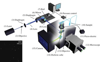
The illumination system is sketched in figure 1. A laser beam (1) is initiated from a Sapphire laser (Coherent Sapphire 488-50) of wavelength 488 nm at output power 350 mW. This paralleled beam goes through an objective with
 $\times \,10$
magnification (2) to be focused on the focal plane. A diaphragm (3) is placed on the same focal plane with
 $10~{\rm\mu}\text{m}$
of diameter to let pass only the focused light. A lens (4) with focal length 150 mm is placed behind the orifice, with its focal plane superposed with that of the
 $\times \,10$
objective. The beam comes out from this lens being parallelled again but with an enlarged diameter at 2 cm. The implementation of (2), (3) and (4) is for producing a perfectly parallelled laser beam with enlarged diameter, and eliminating lights due to unparallelled incidence and diffraction. The parallelled beam goes through a diaphragm (5), which is fixed on the table during the first step of alignment of the laser and serves as a reference point of the beam. The component (6) is a mirror which reflects the beam at 90° and incident onto a lens (8) to be focused on its focal plane; this focal plane is shared by the lens (8) and the objective of the microscope. There is a dichroic filter cube (510 nm) situated between the lens (8) and the objective, in order to reflect the incident laser beam up to the objective. The components (6) and (8) are fixed on a rail in order to be moved together horizontally without relative displacement, the rail is regulated by a homemade Labview program. The fact of moving components (6) and (8) horizontally does not impede the laser beam to be focused on the focal plane of the objective, but results in a displacement of focusing point away from the optical line of the objective, which induces an angle of incidence different from 90° relatively to the microchannel.
Scheme of the TIRF set-up. A laser beam is collimated through a high numerical aperture objective (
 $\times \,100$
,
 $\text{NA}=1.46$
) with an incidence angle higher than the critical angle for total reflection. Laser is focused in the back focal plane of the objective with an achromatic doublet (focal
 $\text{length}=200~\text{mm}$
) and the incidence angle is tunable by displacing a mirror in the optical path. The evanescent wave created within the channel restricts fluorescence to tracers (dots over the glass slide) in the vicinity of the surface, which is collected by the high-speed camera. The image on the left bottom corner is a typical acquisition.

The advantage of using an objective for TIRF measurement relies in the convenience of sending incident light at a supercritical angle without a prism, and retrieving fluorescence information at the same time (see Selvin & Ha Reference Selvin and Ha2008). The objective has magnification
 $\times \,100$
and a high numerical aperture at 1.46. The numerical aperture is expressed by the following equation:
 $$\begin{eqnarray}\text{NA}=n_{i}\sin ({\it\Theta})\end{eqnarray}$$
where
 $n_{i}$
is the refractive index of the working medium of the objective, i.e. immersion oil (
 $n_{i}=1.518$
).
 ${\it\Theta}$
is the half-angle of the maximum light cone (
 ${\it\theta}=74.1^{\circ }$
). The total reflection critical angle at the interface of water and glass slide (refractive index
 $n=1.52$
from Menzel-Gläser) is approximately 61.4° with the refractive index of water at 1.3327; and for the interface of sucrose solution at 40 wt% and glass slide it is 67.1° with the refractive index of sucrose solution at 1.3981. The incidence angle is measured by a glass hemisphere, which projects the light spot onto millimetre paper. This angle
 ${\it\theta}$
is
 $$\begin{eqnarray}{\it\theta}=\arctan (H/L)\end{eqnarray}$$
where
 $L$
is the horizontal distance between the objective and the millimetre paper board. The light spot height
 $H$
is measured with a 1 mm precision, which corresponds to an error of 1 nm on the penetration length, i.e. less than 1 % error on its determination.
Another advantage of using objective with large numerical aperture and oil immersion consists in the increasing number of orders of diffraction collected by the lens, which reduces the size of the Airy diffraction disk and increases the precision at which particle positions are measured.
The expression of the evanescent field we apply reads, within the liquid,
 $$\begin{eqnarray}I=I_{0}\exp (-z/p)\end{eqnarray}$$
in which
 $z$
is the distance from the glass/liquid interface (i.e. the channel wall),
 $p$
is the field depth of penetration usually around 135 nm and
 $I_{0}$
is the intensity of the evanescent field at
 $z=0$
. We use an Andor Neo sCMOS camera for the acquisition of data. It has several advantages. First, it is able to work with a good sensitivity at 16 bit, which means 65 536 grey levels accessible, and so allows the distinction of two slightly different intensities. Second, by using the rolling shutter mode, we can benefit from this lower noise and acquire data at high frame rate (400 f.p.s.), as
 $512~\text{pixels}\times 512~\text{pixels}$
pictures are taken during the experiments, with a 2.5 ms exposure time. Operated in overlay mode, there is no time gap between two successive exposures, so that no information is lost. (The rolling shutter mode works in a way that adjacent rows of pixels are exposed at slightly different moment. This time delay is
 $9.24~{\rm\mu}\text{s}$
. The exposure duration of each line is set at 2.5 ms. This allows reading out of the first lines during the exposure of the following lines. On an image with size
 $512~\text{pixels}\times 512~\text{pixels}$
, the moment of the top and bottom lines being exposed is delayed with respect to the centreline with 2.37 ms. As a consequence, the rolling shutter mode allows each line being exposed in two consecutive images with no time gap.) Third, the camera provides 4 GB of on-head image buffer, which overcomes the limitation of frame rate due to the eventually low write rate of hardware, and enables frame rates up to 400 images per second. Fourth, the camera offers a field-programmable gate array (FPGA)-generated hardware timestamp with the precision of 25 ns, i.e. 1 % of the exposure time, which has a negligible effect on the velocity calculation. Finally, this sCMOS camera has an amplifier for each pixel, so that there might be a slight difference of amplification rate. However, the difference of amplification rate is 0.1 % in intensity, which induces 0.1 % error of altitude calculation, corresponding to 0.1 nm, which is a negligible effect in the experiments. The fluids are injected with a MFCS-FLEX pressure controller by Fluigent. The maximum pressure is 1000 mbar, with 1 mbar precision (0.1 % of full scale). The minimum pressure applied in the water experiment is 20 mbar, which means that the source of error due to the pressure controller introduces an error on the stress calculation of maximum 5 % for water and 1 % for 40 wt% sucrose solution, inducing a maximal error on the deduced viscosity of 5 % and 1 % respectively. Deionized water (DIW) and 40 wt% of sucrose solution in DIW are studied. FluoSpheres particles from Invitrogen (carboxylate modified 100 nm yellow–green fluorescent particles F8803, solid 2 wt%,
 $3.6\times 10^{13}~\text{particles}~\text{ml}^{-1}$
) are used as tracers. Their peak excitation and emission wavelengths are 505 and 515 nm. The particle concentration seeded in 40 wt% sucrose solution and DIW are 0.0004 and 0.002 wt% solid, respectively, so as to have up to 10 particles detected in each frame. The channel dimension is
 $L=8.8~\text{cm}$
in length,
 $w=183~{\rm\mu}\text{m}$
in width and
 $h=18.3~{\rm\mu}\text{m}$
in height. With these dimensions, the hydrodynamic resistance has the right order of magnitude to operate with flow speeds well adapted to our particle tracking system. The channel is designed in a coil shape in order to save space. With a
 $\mathit{Re}$
on the order of
 $10^{-3}$
, inertia is neglected and the small turning points of the channel does not induce any recirculation nor instabilities. Both hydrophilic and hydrophobic surfaces are studied. Hydrophilic surfaces are prepared by treating glass slides with Piranha solution (30 vol% hydrogen peroxide and 70 vol% of sulfuric acid) heated at 300 °C until degassing ends. The obtained slides are bonded to PDMS channels with
 $\text{O}_{2}$
plasma treatment. Hydrophobic surfaces are obtained by coating a layer of
 $n$
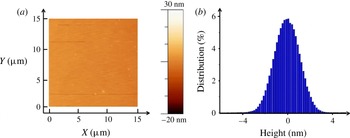
-octadecyltrichlorosilane on a slide treated by Piranha solution (McGovern, Kallury & Thompson Reference McGovern, Kallury and Thompson1994). The coated hydrophobic layer is 20 Å thick according to ellipsometry measurements. The contact angle of a DIW drop on the coated layer is 105°, measured by a surface tension determination set-up KRÜSS DSA30. The roughness of the coated surface is measured by atomic force microscopy (AFM; figure 2): the relative roughness distributes around
 $0\pm 1.3~\text{nm}$
at half-height. The hydrophobic slide is combined with channel printed in NOA (photocurable monomer) (Bartolo et al.
Reference Bartolo, Degré, Nghe and Studer2008). NOA-made channels are preferred to PDMS to avoid the alteration of the hydrophobic coating by the plasma exposition.
State of hydrophobic surface coated on glass slide by
 $n$
-octadecyltrichlorosilane, thickness measured by AFM (a) and RMS (b) indicating the roughness distributes around
 $0\pm 1.3~\text{nm}$
at half-height.

3. Method of measurement of the particle locations and speeds
During the acquisition, for each 5 s long experimental run, 2000 images are taken; and for each applied pressure, 6 runs are carried out to ensure a high enough number of detected particles (around 80 000), which will contribute to the statistics of the data analysis. The measurement of the intensity is the averaged intensity
 $\bar{I}$
over the exposure time of the camera
 ${\it\tau}$
, with
 ${\it\tau}=2.5~\text{ms}$
. In this process, no information on particle trajectory is lost from the observation, since there is a negligible time gap between two consecutive images. This represents a crucial difference with previous work (e.g. Huang et al.
Reference Huang, Guasto and Breuer2006; Li & Yoda Reference Li and Yoda2008). The experimental conditions and characteristic numbers are summarized in table 1. An interesting quantity that we used in the discussion of the results is the shear rate
 $\dot{{\it\gamma}}$
which is determined by the following formula:
 $$\begin{eqnarray}\dot{{\it\gamma}}=\frac{h{\rm\Delta}P}{2{\it\mu}L}\end{eqnarray}$$
where
 ${\rm\Delta}P$
is the applied pressure and
 ${\it\mu}$
the fluid viscosity.
Experimental conditions and non-dimensional numbers. Here,
 $\dot{{\it\gamma}}$
the fluid shear rate. Reynolds number is defined as
 $\mathit{Re}={\it\rho}VH/{\it\mu}$
and Péclet numbers defined as
 $\mathit{Pe}=\dot{{\it\gamma}}r_{0}^{2}/D_{0}$
(Guasto & Breuer Reference Guasto and Breuer2009), where
 $V$
is the average velocity of fluid in the channel,
 ${\it\rho}$
density of the fluid,
 $H$
height of the channel,
 $D_{0}$
diffusion coefficient of particles in the fluids calculated by Stokes–Einstein equation and
 $r_{0}$
the particle radius. Viscosity
 ${\it\mu}$
is measured by conventional rheometer at 20 °C.

A custom-made Matlab program is used to analyse the detected particles intensity and displacements. We use the tracking method developed by Bonneau, Dahan & Cohen (Reference Bonneau, Dahan and Cohen2005). The subpixel
 $x$
and
 $y$
locations are obtained by convoluting the detected intensity spot with a two-dimensional Gaussian template, with standard deviation
 ${\it\sigma}\approx 1.1$
pixels, and discretized on a support of size
 $5~\text{pixels}\times 5~\text{pixels}$
. The accuracy of coordinates determination is 0.1 pixels with a signal-to-noise ratio greater than 10 (Bonneau et al.
Reference Bonneau, Dahan and Cohen2005). This represents a spatial uncertainty of 6 nm. In this study of TIRF, since the velocity close to the wall is small, and the time delay between two frames is short, the particle image shift of one particle between two frames is small compared with the image distance between two different particles. The system works in low-concentration particle tracking velocimetry (PTV) mode, considering that the number of particles detected in one image is around 10 in a window of
 $33~{\rm\mu}\text{m}\times 33~{\rm\mu}\text{m}$
. Thus, an algorithm is implicated to identify the same particle which appeared in two successive images with a nearest-neighbour search (Guasto & Breuer Reference Guasto and Breuer2009), taking into account the estimated displacement and the diffusion effect. The technique is efficient, and mismatches are extremely rare events.
After particle identification, displacement between two successive frames can be calculated with a theoretical precision of
 $6\sqrt{2}\approx 8~\text{nm}$
. The time-averaged velocities
 $\bar{V}_{X}$
and
 $\bar{V}_{Y}$
are calculated by displacement divided by time 2.5 ms. The time-averaged intensity
 $\bar{I}$
is subtracted by camera background noise, and then normalized by the laser-only intensity at the pixel position. The apparent intensity of one identified particle
 $\bar{I}_{app}$
is the average between two successive frames,
 $\bar{I}_{app}=(\bar{I}_{1}+\bar{I}_{2})/2$
, where
 $\bar{I}_{1}$
and
 $\bar{I}_{2}$
are the time-averaged intensity measured in the first frame (called frame 1) and in the next one (called frame 2), respectively. In general, because of Brownian motion, the particle in frame 1 has not the same altitude as in frame 2. In order to check the effect of the altitude fluctuations on the results, we have compared velocity profiles constructed with a selection of particles travelling less than 50 nm in altitude between frames 1 and 2, with profiles obtained with particles travelling up to 200 nm in altitude between the same frames. We found that the two profiles are undistinguishable. We thus did not introduce any rule of selection of particles at this level.
The apparent altitude
 $\bar{z}_{app}$
of the particle is inferred by using the following expression derived from (2.3):
 $$\begin{eqnarray}\bar{z}_{app}=p\log \frac{I_{0}}{\bar{I}_{app}}\end{eqnarray}$$
in which
 $I_{0}$
is the intensity emitted by a particle located at the wall, a crucial parameter deserving a separate measurement (see § 6).
After these measurements are carried out for each individual particle, we proceed to statistical averaging over many particles. First, all of the particles are sorted out according to their apparent altitudes
 $\bar{z}_{app}$
. A box is an interval, along the
 $z$
axis, which contains particles whose apparent altitude belongs to the interval. The box sizes represents the spatial precision at which the velocity profile is measured. Throughout the experiments, we take box sizes of the order of a few nanometres for distances larger than 200 nm from the wall. At less than 200 nm from the wall, box sizes can reach 50 nm. The reason is that we impose that each box includes
 $N=1000$
particles, so as to guarantee statistical convergence. Thereby, since there are only a few particles very close to the wall, the box sizes must be increased in that region. Note that, thanks to temporal and spatial averaging, the accuracy on the determination of the averaged particle altitudes, and therefore the sizes of the boxes we take, is much smaller than the standard deviation of the Brownian movement.
The statistically averaged velocities and apparent altitudes, calculated in each box, are determined by the relations
 $$\begin{eqnarray}\langle \bar{V}_{X}\rangle =\frac{1}{N}\mathop{\sum }_{N}\bar{V}_{X};\quad \langle \bar{V}_{Y}\rangle =\frac{1}{N}\mathop{\sum }_{N}\bar{V}_{Y};\quad \langle \bar{z}_{app}\rangle =\frac{1}{N}\mathop{\sum }_{N}\bar{z}_{app}\end{eqnarray}$$
 $z$
in which
 $X$
and
 $Y$
are respectively the streamwise and cross-stream coordinates, and
 $\bar{V}_{X}$
and
 $\bar{V}_{Y}$
the corresponding time averaged speeds. The summations are carried out in each box over the 1000 particles belonging to it. The raw velocity profile is defined as
 $\langle \bar{V}_{X}\rangle$
versus
 $\langle \bar{z}_{app}\rangle$
.
At this stage, we can estimate the measurement accuracy of the apparent altitude using (3.2). A first source of error on
 $z_{app}$
comes from
 $I_{0}$
(see below) and
 $p$
. Both are determined with a 2 nm precision. The second source of error, and the most important, is statistical. From the above discussion, with a 95 % confidence interval and 1000 particles, the error on
 $z_{app}$
is 2 nm. To summarize, the error on
 $z_{app}$
is of the order of 2 nm and that of particle image displacement is 5 nm.
4. Langevin modelling of the particle trajectories and intensity measurements
In this section, we describe the stochastic Langevin equations we used to interpret our measurements. We used the same approach as Huang et al. (Reference Huang, Guasto and Breuer2006). We consider here a population of spherical particles, with a mean radius
 $r_{0}$
and size dispersion
 ${\it\sigma}_{r}$
, assuming a normal distribution for the radius
 $r$
:
 $$\begin{eqnarray}p_{R}(r)=\frac{1}{{\it\sigma}_{r}\sqrt{2{\rm\pi}}}\exp -\frac{((r/r_{0})-1)^{2}}{2{\it\sigma}_{r}^{2}}.\end{eqnarray}$$
These particles are transported by a pure no-slip shear flow
 $V(z)=\dot{{\it\gamma}}z$
(where
 $\dot{{\it\gamma}}$
is the shear rate) close to a wall located at
 $z=0$
.
The stochastic Langevin equations assign coordinates
 $x(t)$
,
 $y(t)$
,
 $z(t)$
, to each particle centre at time
 $t$
. The particles interact with the surface charges at the wall. We must introduce zeta potentials
 ${\it\zeta}_{p}$
and
 ${\it\zeta}_{w}$
for the particles and the wall, respectively, to describe this effect. We neglect van der Waals forces, which act on scales much smaller than those we consider here (we checked that adding them does not affect the results of the paper). For the sake of simplicity, we work with dimensionless quantities, using the following dimensionless variables
 $X=x/r_{0}$
,
 $Y=y/r_{0}$
,
 $Z=z/r_{0}$
and
 $T=t/(r_{0}^{2}/D_{0})$
. Thus,
 ${\it\delta}T={\it\delta}t/(r_{0}^{2}/D_{0})$
is the dimensionless time increment taken for the integration of the trajectories. The discretized equations that describe the particle dynamics, originally written by Ermak & McCammon (Reference Ermak and McCammon1978), are
 $$\begin{eqnarray}\displaystyle & \displaystyle X_{i+1}=X_{i}+F(Z_{i})~\mathit{Pe}~Z_{i}~{\it\delta}T+S\left(0,\sqrt{2{\it\beta}_{x}(Z_{i}){\it\delta}T}\right) & \displaystyle\end{eqnarray}$$
 $$\begin{eqnarray}\displaystyle & \displaystyle Y_{i+1}=Y_{i}+S\left(0,\sqrt{2{\it\beta}_{y}(Z_{i}){\it\delta}T}\right) & \displaystyle\end{eqnarray}$$
 $$\begin{eqnarray}\displaystyle & \displaystyle Z_{i+1}=Z_{i}+\left.\frac{\text{d}{\it\beta}_{z}}{\text{d}Z}\right|_{Z_{i}}{\it\delta}T+H(Z_{i}){\it\beta}_{z}(Z_{i}){\it\delta}T+S\left(0,\sqrt{2{\it\beta}_{z}(Z_{i}){\it\delta}T}\right) & \displaystyle\end{eqnarray}$$
 ${\it\beta}_{x}$
and
 ${\it\beta}_{y}$
) and cross-stream (
 ${\it\beta}_{z}$
) diffusion coefficients are defined by
 $$\begin{eqnarray}\displaystyle & \displaystyle {\it\beta}_{x}(Z)={\it\beta}_{y}(Z)=1-{\textstyle \frac{9}{16}}Z^{-1}+{\textstyle \frac{1}{8}}Z^{-3}-{\textstyle \frac{45}{256}}Z^{-4}-{\textstyle \frac{1}{16}}Z^{-5}+O(Z^{-6}), & \displaystyle\end{eqnarray}$$
 $$\begin{eqnarray}\displaystyle & \displaystyle {\it\beta}_{z}(Z)=\frac{6(Z-1)^{2}+2(Z-1)}{6(Z-1)^{2}+9(Z-1)+2}. & \displaystyle\end{eqnarray}$$
The other dimensionless functions are defined by the following expressions:
 $$\begin{eqnarray}F(Z_{i})=\frac{U(z_{i})}{z_{i}\dot{{\it\gamma}}};\quad H(Z_{i})=\frac{F_{pw}(Z_{i})r_{0}}{k_{B}{\it\Theta}};\quad \mathit{Pe}=\frac{\dot{{\it\gamma}}{r_{0}}^{2}}{D_{0}}\end{eqnarray}$$
in which
 $U(z_{i})$
is the fluid longitudinal velocity of a particle at the height
 $z_{i}$
.
Assuming that the wall particle interaction is described by Derjaguin–Landau–Verwey–Overbeek (DLVO) theory, we obtain the following expression for
 $F_{pw}(Z_{i})$
:
 $$\begin{eqnarray}F_{pw}^{el}=4{\rm\pi}{\it\epsilon}\frac{r_{0}}{{\it\lambda}_{D}}\left(\frac{k_{B}{\it\Theta}}{e}\right)^{2}\left(\frac{\hat{{\it\zeta}_{p}}+4{\it\gamma}{\it\Omega}{\it\kappa}r_{0}}{1+{\it\Omega}{\it\kappa}r_{0}}\right)\left[4\tanh \left(\frac{\hat{{\it\zeta}_{w}}}{4}\right)\right]\exp \left(-\frac{z-r_{0}}{{\it\lambda}_{D}}\right)\end{eqnarray}$$
where
 $$\begin{eqnarray}\hat{{\it\zeta}_{p}}=\frac{{\it\zeta}_{p}e}{k_{B}{\it\Theta}};\quad \hat{{\it\zeta}_{w}}=\frac{{\it\zeta}_{w}e}{k_{B}{\it\Theta}};\quad {\it\gamma}=\tanh \left(\frac{\hat{{\it\zeta}_{p}}}{4}\right);\quad {\it\Omega}=\frac{\hat{{\it\zeta}_{p}}-4{\it\gamma}}{2{\it\gamma}^{3}}\end{eqnarray}$$
and in which
 $k_{B}$
is the Boltzmann constant,
 ${\it\epsilon}={\it\epsilon}_{w}{\it\epsilon}_{0}$
is the dielectric constant of water,
 ${\it\zeta}_{p}$
and
 ${\it\zeta}_{w}$
are zeta potentials of the particles and the wall, respectively, and
 ${\it\lambda}_{D}$
is the Debye length.
The stochastic displacement of the particles due to Brownian motion is represented by the
 $S$
function, following a normal distribution with a zero mean value and the dimensionless diffusion length
 $L=\sqrt{2{\it\beta}(Z){\it\delta}T}$
as its standard deviation.
The total fluorescence intensity
 $I$
emitted by the particle at time
 $t_{i}$
must then be calculated. Here, we consider that the particle is at some distance
 $z_{f}$
from the object plane of the objective. Bleaching is neglected, owing to the fact that the time of interest (2.5 ms) is much smaller than the fastest bleaching time (see § 6). The total intensity emitted by the particle, being proportional to the incident light intensity it collects, is thus given by the following expression:
 $$\begin{eqnarray}I(Z)=I_{0}\left(\frac{r}{r_{0}}\right)^{3}\exp \left(-\frac{z}{p}\right)\frac{1}{1+\left(\frac{z-z_{f}}{P_{c}}\right)^{2}}\end{eqnarray}$$
where the parameters have the following definition.
-
(i) We use
$I_{0}$
to denote the intensity emitted by a particle of radius
$r_{0}$
located at the wall, i.e. at
$z=r_{0}$
, whose centre is placed at the image plane of the camera sensor, i.e. at
$z=z_{f}$
. -
(ii) We use
$P_{c}$
to denote the depth of field of the optical system that images the particles (Joseph & Tabeling Reference Joseph and Tabeling2005). This parameter is estimated with the following formula (4.8): (4.8)in which
$$\begin{eqnarray}P_{c}=\frac{n{\it\lambda}_{0}}{\text{NA}^{2}}+\frac{na}{\text{NA}\,M}\end{eqnarray}$$
$n$
is the refractive index of the working medium
$(n=1.518)$
,
${\it\lambda}_{0}$
the excitation wavelength (
${\it\lambda}_{0}=488~\text{nm}$
),
$a$
the pixels size of the CMOS sensor (
$a=6.5~{\rm\mu}\text{m}$
), NA the numerical aperture of the objective (
$\text{NA}=1.46$
) and
$M$
the magnification (
$\times \,100$
). The formula gives 348 nm for
$P_{c}$
. Here,
$z_{f}$
represents the position of the image plane of the camera sensor, which is estimated to be 350 nm. The choice of this value is supported by calibration experiments (see appendix A). The position of the focal plane has 50 nm accuracy. According to (4.7), this error on focal plane position deduces 2 % of error on detected intensity, which corresponds to 2 nm on altitude determination. The effect of defocusing has not been considered thus far by the previous investigators, which seems justified by the fact that their objectives have smaller numerical apertures.


The procedure we use mimics rigorously the experimental methodology. It decomposes into the following steps.
-
(i) We generate particles whose initial positions span a range of altitudes between 100 and 700 nm, with uniform distributions. This interval corresponds to the range of altitudes within which particles are detected in the experiment. Outside this range, the particles are not detected either because of the existence of a depletion or the signal they emit is indistinguishable from the noise.
-
(ii) Each particle wanders in space, and reaches some position (say, 1) after a time
${\it\tau}$
equal to the exposure time of the camera, i.e. 2.5 ms. This position is calculated by using (4.2). After another time
${\it\tau}$
, the particle reaches a second position (say, 2) which is calculated in the same way. -
(iii) For each particle, the intensity
$I(Z)$
is temporally averaged between the initial time
$t=0$
and
$t=2{\it\tau}$
, the result being
$I_{app}$
. A similar procedure applies for the altitude, leading to
$z_{mean}$
and for the horizontal coordinates of the particle. -
(iv) The apparent altitude
$z_{app}$
is calculated similarly as in (3.2). The formula is (4.9)Note that
$$\begin{eqnarray}z_{app}=r_{0}+p\log \frac{I_{0}}{I_{app}}.\end{eqnarray}$$
$z_{app}$
is generally different from
$z_{mean}$
.
-
(v) The horizontal displacement vector of the particle between its mean positions 1 and 2 is calculated. The components of this vector are divided by the separation time (i.e.
${\it\tau}$
) to obtain the components of the apparent fluid speed,
$V_{xapp}$
and
$V_{yapp}$
as a function of
$z_{mean}$
. -
(vi) Boxes similar to the experiment are defined (see § 3). The quantities or interest (altitudes, speeds) are further averaged out statistically over thousands of particles located in each boxes. Distributions are also obtained.


A final remark concerns the stationarity of our simulations. They are not stationary, since in the course of time, the particles tend to diffuse away. Nevertheless, the escape is extremely slow (its characteristic time is a fraction of seconds, i.e. several hundreds of times the time we consider here,
 ${\it\tau}$
). The escape process is also slow with respect to the speed of establishment of the Debye layer, which takes only a fraction of
 ${\it\tau}$
to build up. Therefore, on the time scales we consider in the simulations, the leak of particles we evoke here can be neglected.
5. Using Langevin simulation to correct altitudes and speeds
Now we make use of the simulations to discuss the relation between the apparent altitude
 $z_{a}=\langle z_{app}\rangle$
and the apparent longitudinal speed
 $V_{a}=\langle V_{xapp}\rangle$
(where the brackets mean statistical averaging in the boxes). In fact, each apparent quantity is a function of
 $\langle z_{mean}\rangle$
. Therefore, by eliminating
 $\langle z_{mean}\rangle$
, we can plot
 $V_{a}$
in function of
 $z_{a}$
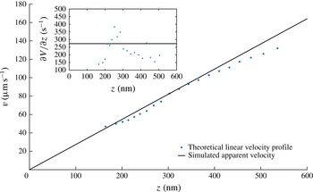
, thus mimicking the experimental measurements we perform. The plot is shown in figure 3.
Simulated velocity profiles of sucrose 40 wt% solution on an hydrophilic surface for an inlet pressure
 $p=195~\text{mbar}$
. The parameters of the simulation are
 ${\it\lambda}_{D}=22~\text{nm}$
,
 $P_{c}=348~\text{nm}$
,
 $z_{f}=300~\text{nm}$
and
 $p=124~\text{nm}$
. The inset shows the local slope of the velocity profile.

One sees that the apparent profile
 $V_{a}(z_{a})$
departs from the true profile
 $V(z_{a})=\dot{{\it\gamma}}z_{a}$
. Close analysis shows that as a whole, the apparent profile is shifted towards the right by a few nanometres, for reasons related to the coupling between Brownian fluctuations and convexity of the function
 $I(z)$
. On the other hand, the lower part of the apparent profile is curved upwards. This is due to the depletion in particles in the Debye layer. More explicitly, the explanation is as follows: with the values we have taken in the simulations shown in figure 3, the Debye layer thickness is 22 nm. Under such conditions, the depletion in particles is perceptible up to 150 nm. Particles located in the depleted layer develop smaller excursions near the wall than far from it. It follows that their apparent altitude, calculated from the nonlinear equation (4.9), is underestimated, while their apparent speed is overestimated. These particles thus stand apparently closer to the wall than they are, and move apparently faster than they do. This artefact gives rise to an apparent profile
 $V_{a}(z_{a})$
that tends to level off as the wall is approached.
Another deviation between the apparent and expected profiles is visible at large distances, where the upper part of the profile is curved downwards. This effect originates in the fact that as we move farther from the wall, the particles become more and more unfocused and consequently, they seem farther than they are. A consequence of defocusing is a slope reduction (down to 20 %), which gives rise to an overestimate of the in situ viscosity when determined from formula (9.1). Note that these biases are small in amplitude. The consequence is that we do not need an outstanding accuracy on the calculation of the biases to correct the experimental data.
In practice, we use the function
 $V_{a}(z_{a})$
to convert apparent velocity profiles into corrected profiles, which are expected to approach the ‘true’ velocity profiles.
6. Experimental determination of
$I_{0}$

The parameter
 $I_{0}$
is crucial and necessitates an accurate measurement. In order to measure this parameter, we analysed populations of particles physically adsorbed to the wall, thus located at
 $z=r$
. Adsorption of many particles onto the wall is achieved by adding
 $0.05~\text{M}$
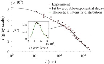
NaCl to the working fluid, thus lowering the repelling electrostatic barrier between the particle and the wall. In our method, which is different from Li & Yoda (Reference Li and Yoda2010), we first turn off the laser, maintain a flow and wait for a few minutes (i.e. in the dark). This time is sufficient for the adsorption process to reach an equilibrium state, where all particles are immobilized. Then we turn the laser on, tune manually the objective position so as the particles lie in the focal plane of the TIRF objective. Throughout the procedure, a video is recorded so that the instant at which the laser is switched on, along with the time at which the first well-focused image of the particles is captured are known with a 23 ms accuracy. No significant amount of particles gets adsorbed to the wall nor desorbs during the time the analysis is carried out. This hypothesis is checked directly on the video. The inset of figure 4 shows an intensity distribution obtained 138 ms after the laser is switched on.
Temporal decay of the intensity
 $I_{B}(t)$
emitted by particles physically adsorbed onto the wall, whose centre are thereby approximately located at
 $z=r$
. Experimental results are fitted by (6.3) which corresponds to double-exponential photo-bleaching kinetics (Song et al.
Reference Song, Hennink, Young and Tanke1995, Reference Song, van Gijlswijk, Young and Tanke1997), with
 $A$
,
 $B$
,
 $t_{1}$
and
 $t_{2}$
as free parameters. The fit parameters are
 $A=2283\pm 359$
grey values,
 $B=6300\pm 223$
grey values,
 $t_{1}=22.4\pm 9.5$
ms and
 $t_{2}=675\pm 49~\text{ms}$
. The fit includes data obtained at
 $t<1~\text{ms}$
. In the inset, the (red online) dots represent, for time
 $t=138~\text{ms}$
, the intensity distribution emitted by the population of particles located at the surfaces; in the same inset, the (green online) line is a fit based on (6.2), from which
 $I_{B}(t)$
and
 ${\it\sigma}_{r}$
are determined.

Such a distribution can be analysed theoretically. Assuming that the bleaching process is the same for all of the particles, the intensity
 $I$
emitted by a particle of size
 $r$
, located at
 $z=r$
, and illuminated by the laser beam for a time
 $t$
, is given by the formula
 $$\begin{eqnarray}I=I_{B}(t)\left(\frac{r}{r_{0}}\right)^{3}\end{eqnarray}$$
in which
 $I_{B}(t)$
is a function that characterizes the bleaching process, assumed to apply uniformly on the particle population, independently of their sizes. In this expression, we do not take into account the fact that the particles, being of different sizes, have their centres located at different distances from the wall and therefore are illuminated with slightly different intensities. The corresponding error is on the order of
 $({\it\sigma}_{r}r/p)^{2}$
i.e.
 $10^{-4}$
. Assuming further a normal distribution for the particle size, with standard-type deviation
 ${\it\sigma}_{r}$
, one obtains the probability density function (p.d.f.) of the intensity emitted by an ensemble of particles located at
 $z=r$
at time
 $t$
:
 $$\begin{eqnarray}p_{W}(I,t)=\frac{r_{0}}{3I_{B}(t){\it\sigma}_{r}\sqrt{2{\rm\pi}}}\left(\displaystyle \frac{I_{B}(t)}{I}\right)^{2/3}\exp -\frac{\left(\left(\displaystyle \frac{I}{I_{B}(t)}\right)^{1/3}-1\right)^{2}}{2{\it\sigma}_{r}^{2}}.\end{eqnarray}$$
Our expression is slightly different from Huang et al. (Reference Huang, Guasto and Breuer2006), because we restored a factor
 $I^{-2/3}$
coming from a variable change, that was not taken into account. The inset of figure 4 shows that this distribution agrees well with the experiment. By comparing the theory and the experiments, we can extract
 ${\it\sigma}_{r}$
and
 $I_{B}(t)$
at each time. Regarding
 ${\it\sigma}_{r}$
, the values range between 8 % and 9 % at all times, which is compatible with the data provided by the constructor (5 % for the size dispersity). As mentioned in Huang et al. (Reference Huang, Guasto and Breuer2006), the standard deviation we obtain incorporates fluctuations in the particle size, number of fluorophores and quantum efficiencies. This may explain why it stands above the sole size dispersity stated by the constructor.
The evolution of
 $I_{B}(t)$
with time is shown in figure 4. We obtain a double-exponentially decreasing function, well represented by the following formula:
 $$\begin{eqnarray}I_{B}(t)=A\text{e}^{-t/t_{1}}+B\text{e}^{-t/t_{2}}.\end{eqnarray}$$
This behaviour reflects that, in the range of time we consider, two time constants are needed to describe the bleaching process, consistently with the literature (Song et al.
Reference Song, Hennink, Young and Tanke1995, Reference Song, van Gijlswijk, Young and Tanke1997) and at variance with Li & Yoda (Reference Li and Yoda2008). Figure 4 is important for the measurement we make, because it allows to check that the direct measurement of
 $I_{0}$
(i.e. that done at
 $t<1~\text{ms}$
, not represented on the figure), is in excellent agreement with the value
 $I_{B}(0)$
obtained with the fit. In practice, by repeating measurements at small times, the errors on the direct measurement of
 $I_{0}$
are estimated on the order of
 $\pm 123$
grey levels, which, translated in
 $z$
-position by using formula (2.3), leads to a
 $\pm 2~\text{nm}$
accuracy.
In Li & Yoda (Reference Li and Yoda2008, Reference Li and Yoda2010) the photo bleaching kinetics of fluorescent particles was not analysed with such a degree of precision. This induced a substantial error on the average value of
 $I_{0}$
, and therefore on the measurement of the slip length.
7. Analysis of the intensity distributions and comparison with the Langevin simulations
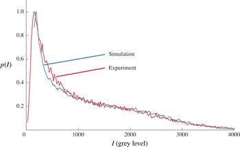
The analysis of intensity distributions of populations of particles seeding the flow allows us to confront our simulation to the experiment. The distributions shown in figure 5 represent an experiment made with a sucrose solution. The distribution is strongly skewed. There are sharp peaks on the left side and bumps on the right wing.
Experimental (red line) and related simulated (blue line) intensity distributions in the case of 40 wt% sucrose solution. Both situations correspond to an inlet pressure of 140 mbar. The simulation parameters are
 ${\it\lambda}_{D}=22~\text{nm}$
,
 $P_{c}=348~\text{nm}$
,
 $z_{f}=300~\text{nm}$
and
 $p=124~\text{nm}$
.

The left side of the distribution represents the contributions of the dimmest particles, i.e. those located far from the wall. If particles were uniformly distributed in space, the evanescent form of the intensity field would induce a hyperbolic function for the intensity distribution, which is consistent with the observed shapes of the central part of
 $p(I)$
. Below a certain level, no particle is detected anymore, and the distribution level collapses. The largest intensity levels probe the closest distances to the wall. The abrupt decrease of
 $p(I)$
at high intensity levels is linked to the existence of depleted layers in the vicinity of the wall. These depleted layers result from the action of hindered diffusion and electrostatic repulsion.
The simulation represents well the overall shape of the observed distributions. There are some discrepancies on the left side of the distribution, where the distribution of the dimmest particles seem to be imperfectly reproduced by the theory. We suggest that the discrepancy is due to the crude modelling of the conditions for which the particles cease to be observable by the camera. On the other hand, there are only small differences on the right part of the distribution, which correspond to the brightest particles, i.e. those located closer to the wall. This suggests that the simplifications made in the theoretical representation of this region are acceptable. One weakness of the DLVO theory we used is that the particles are assumed pointwise, while they occupy a significant fraction of the Debye layer. Another weakness is that some parameters (such as the
 ${\it\zeta}$
potentials of the walls and particles) are poorly known. Still, from the viewpoint of the intensity distributions, these approximations seem acceptable.
As a whole, the agreement can be considered as satisfactory. This is an important observation, which supports the idea that our Langevin model represents well the experiment, and thereby can provide reliable estimates of the existing biases. We also tested the robustness of the agreement with respect to changes in the parameters of the simulations. The lower range of intensities is sensitive to the size of the pack of particles we took for prescribing the initial conditions of the simulation. Likewise, in the upper range of intensity levels, a similar comment can be made regarding the sensitivity of the form of the distribution to the choice of the Debye layer thickness
 ${\it\lambda}_{D}$
. Nonetheless, although quantitative differences may exist when the simulation parameters are not adequately chosen, the structures of the calculated distributions shown in figure 5 are robust. Moreover, changing the aforementioned parameters within a realistic range of values does not affect the velocity profiles outside the Debye layer. As a consequence, for the rest of the paper, we will concentrate ourselves on a range of altitudes lying between 200 and 600 nm for sucrose, 150 and 500 nm for water, for which the particles are sufficiently far from the wall to be insensitive to the detailed characteristics of the Debye layer, and more generally, for which the simulated velocity profiles are robust with respect to moderate changes of the simulation parameters.
8. Analysis of the velocity distributions and comparison with the Langevin simulation
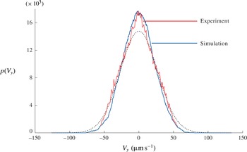
A typical transverse velocity distribution (i.e. along
 $y$
), averaged across the
 $z$
interval 100–600 nm, is shown in figure 6 and compared with the Langevin simulation. Both agree well.
Transverse velocity
 $V_{y}$
distribution. Red and blue lines correspond to experimental and simulated data, respectively. The dotted line is the Gaussian distribution with standard deviation
 ${\it\sigma}_{v}=(2D/{\it\tau})^{1/2}$
.

It is interesting to note that
 $V_{y}$
distribution is more peaked than a Gaussian curve, indicating that small
 $V_{y}$
events are more probable than they would be for a Gaussian process. In fact, here, we look at the travelled distance along
 $y$
made by a large number of particles launched at the origin, after a time
 ${\it\tau}$
. Within the range of time we considered, the process apparently keeps the memory of the initial condition, giving rise to a cusp of the p.d.f. around the origin. Since the distribution is not Gaussian, the diffusion constant associated to the
 $V_{y}$
distribution, is given by the following formula:
 $$\begin{eqnarray}D=\frac{{{\it\sigma}_{v}}^{2}{\it\tau}}{{\it\alpha}}\end{eqnarray}$$
with
 ${\it\sigma}_{v}$
being the standard deviation corresponding to the Gaussian distribution and
 ${\it\alpha}\approx 1.2$
. Applying this formula in the experiments, we found diffusion constants in satisfactory agreement with the expectations.
9. Raw velocity profiles and raw viscosities
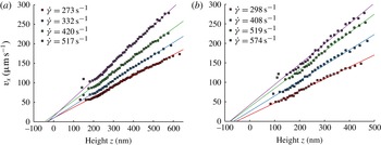
The raw velocity profiles
 $V_{x}(z_{a})$
are shown in figure 7 for the sucrose solution and water pressures, as a function of the apparent altitude
 $z_{a}$
. These profiles represent the raw data we obtained, i.e. those without corrections. Between 200 and 500 nm, the profiles are approximately linear in
 $z_{a}$
. This is explained by the fact that on the scales we consider, the curvature of the Poiseuille profile is not visible and consequently, the profiles must be straight.
Uncorrected velocity profiles obtained with a 40 wt% sucrose solution, over a hydrophilic surface (a) and with water over a hydrophobic surface (b) for different pressures. Linear fits are made between 200 and 600 nm for sucrose and 150 and 500 nm for water.

Nonetheless, on looking in more detail, there is a systematic tendency to curve downwards above 500 nm. This is mainly due to defocusing, that weakens the intensity emitted by the particles and, in turn, increases their apparent altitude. Below 200 nm, the profiles tend to level off. This effect is due to the existence of a depletion zone close to the Debye layer, that favours a systematic underestimate in the measurement of the particle altitude and overestimated of speeds, as explained previously. According to the simulation, the levelling-off effect is more pronounced when the Debye length is increased. This effect tends to vanish out as we move away from the walls, where the electrostatic force is out of scale and particle concentration distribution tends to be homogeneous.
From the measurements of the profile slopes, in regions located between, typically, 200 and 600 nm (where both electrostatic and defocusing biases are reduced), one may determine an apparent viscosity
 ${\it\mu}_{a}$
, through the formula (see (3.1)):
 $$\begin{eqnarray}{\it\mu}_{a}=\frac{h{\rm\Delta}P}{2\dot{{\it\gamma}}L}.\end{eqnarray}$$
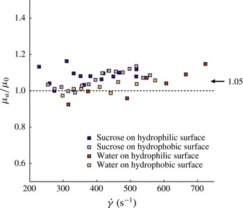
The measurements are shown in figure 8. There are fluctuations (presumably linked to the
 $\pm 50~\text{nm}$
uncertainties on the determination of the location of the focal plane) but it appears that viscosities systematically tend to stand above the expected values, by an amount of the order of 5 %. The existence of this bias along with the order of magnitude of its importance, supports the analysis made in a precedent section.
Uncorrected measurements of the ratio between the in situ apparent viscosity
 ${\it\mu}_{a}$
(see (9.1)) over the bulk viscosity
 ${\it\mu}_{0}$
, determined independently with a rheometer. The mean deviation between the apparent and the bulk viscosity is 5 %.

10. Corrected velocity profiles and corrected viscosities
Figures 9 and 10 show the same set of data, but corrected, using formulas based on figure 3. The corrected data is close to the raw data, typical differences being on the order of 10 %. The corrected profiles are straight above approximately 200 nm, indicating that the tendency to curve down, as a result of defocusing, has been captured by the Langevin simulation and satisfactorily corrected. Moreover, the tendency to level off at small altitudes is less pronounced on the corrected than on the raw profiles.
Corrected velocity profiles obtained with sucrose solution 40 wt%, on the hydrophilic surface (a) and the hydrophobic surface (b), for different pressures. The linear fit are calculated between 200 and 600 nm. For hydrophilic walls, all profiles converge to a no-slip condition; with hydrophobic walls, they confirm the existence of slippage, with a slip length of
 $35\pm 5~\text{nm}$
.

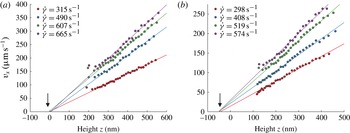
Corrected velocity profiles obtained with water, on the hydrophilic surface (a) and the hydrophobic surface (b), for different pressures. The linear fits are calculated between 250 and 500 nm for the hydrophilic case and 150 and 500 nm for the hydrophobic one.

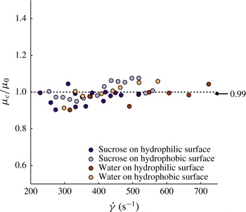
The viscosities, obtained by using formula (9.1), with shear rates estimated by fitting linearly the corrected profiles, are significantly closer to the expected values, the remaining discrepancy being of the order of 1 %, as shown in figure 11. These results, associated to the remarks previously made on the shapes of the corrected profiles, support the validity of our method of correction.
Data showing corrected values of the in situ measured viscosity
 ${\it\mu}_{c}$
divided by the bulk viscosity
 ${\it\mu}_{0}$
determined independently. The graph includes data obtained with hydrophilic and hydrophobic walls. The mean statistical deviation is 1 %.

11. Slip length measurements
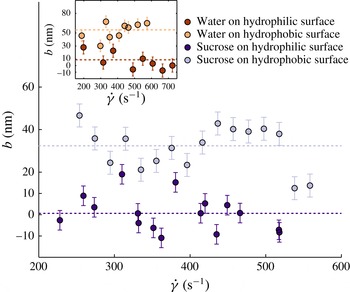
We are now in a position to carry out slip length measurements. As for the viscosity, slip lengths are obtained by fitting the corrected velocity profiles with straight lines, usually restricting ourselves to the 200–600 nm range, and extrapolate them down to the
 $z$
axis. The (extrapolated) slip lengths are then measured as a function of the shear rate by localizing the intersections of this line with the horizontal axis, using the fit expressions.
Slip lengths measurements, obtained with the sucrose solution. The inset is the case of water. In all cases, one can easily detect a difference between hydrophilic (dark dots) and hydrophobic (light dots) walls.

The results are plotted in figure 12, for hydrophilic, hydrophobic walls, using water and sucrose. For hydrophilic walls, one obtains, both for water and sucrose solutions, a slip length indistinguishable from zero. For hydrophobic walls, the slip lengths are clearly above the horizontal axis. It thus appears that the nature of the wetting property of the wall (i.e. whether it is hydrophilic or hydrophobic) is well captured by our slip length measurements, a result still not established firmly in the literature with TIRF-based velocimetry, owing to the importance of the experimental uncertainties reported in the corresponding papers.
Taking the rule of 95 % confidence interval, and neglecting possible variations with the shear rate of the measured quantities, an hypothesis being acceptable owing to the small range of flow rate we explored, we obtain
 $1\pm 5~\text{nm}$
and
 $9\pm 10~\text{nm}$
for hydrophilic walls (for the case of sucrose and water, respectively) and
 $32\pm 5~\text{nm}$
and
 $55\pm 9~\text{nm}$
for hydrophobic walls (again for sucrose and water, respectively), as shown in table 2. This estimate of the errors does not include that made on
 $I_{0}$
, which was found close to 2 nm (see § 6), and which therefore can be neglected if we assume statistical independency. The hydrophilic data agrees well with the literature (Cottin-Bizonne et al.
Reference Cottin-Bizonne, Cross, Steinberger and Charlaix2005). Hydrophobic slip lengths stand in the right order of magnitude with published works: (Huang et al.
Reference Huang, Guasto and Breuer2006; Joly et al.
Reference Joly, Ybert and Bocquet2006; Vinogradova et al.
Reference Vinogradova, Koynov, Best and Feuillebois2009).
Summary of our measurements made on slip lengths and viscosity errors.

12. Conclusion
The first outcome of this paper is about the technique. We showed that nanoPTV technique, associated to Langevin stochastic calculations, achieves accuracies (
 $\pm 5~\text{nm}$
) on the determination of slip lengths, while delivering a local information on the structure of the velocity profile. For the domain of nanoPTV technique, this marks a substantial progress as compared with the state of the art, where error bars were such that it was difficult to draw out a firm conclusion on the existence of slippage over hydrophilic or hydrophobic walls. Other methods lead to comparable accuracies but, being global, they do not provide information on the local structure of the flow profile.
Our work also suggests that the exploration of distances less than 200 nm seems difficult. Below 200 nm, the particles are subjected to a variety of influences (diffusive drift, electrostatic field, strong particle concentration gradients, etc.) that make the interpretation of their trajectories challenging; consequently the relationship between the average particle movement and the flow speed, along with their apparent altitude and their true distance to the wall, are difficult to quantify. In this region, the biases tend to have an amplitude comparable with the signal. This aspect has been overlooked in Bouzigues et al. (Reference Bouzigues, Tabeling and Bocquet2008), coauthored by one of the authors of the present paper (P.T.).
We envision applications of our approach to non-Newtonian flows, such as polymer solutions, microgels concentrated suspensions or living micelles, where the technique can readily be applied. These systems, in particular the polymer solutions, deserve a confirmation of slippage measurements made in the past with less-sophisticated techniques.
Moreover, our work leads to interesting results concerning slip lengths. The slip lengths we found for hydrophobic surfaces have the same order of magnitude as the literature. They also stand much above the numerical simulations. We thus confirm the unresolved discrepancy between experiments and numerical simulations (Cottin-Bizonne et al. Reference Cottin-Bizonne, Cross, Steinberger and Charlaix2005). It challenges our understanding of the flow dynamics at nanometric distances from an interface, which in turn questions our ability to understand the physics of transport at solid/liquid interfaces in many systems, including natural ones. Owing to its importance, this unresolved issue deserves being addressed experimentally with different techniques, owing to the formidable difficulties that must be faced to perform quantitative measurements in a range of scales that touch or pertain to the nanofluidic realm.
Acknowledgements
The authors thank L. Bocquet, E. Charlaix, C. Cottin-Bizonne, T. Kitamori, D. Lohse, Z. Silber-Li, M. Tatoulian and C. Ybert for fruitful discussions and exchanges. Support from AEC, ESPCI, CNRS and UPMC is acknowledged.
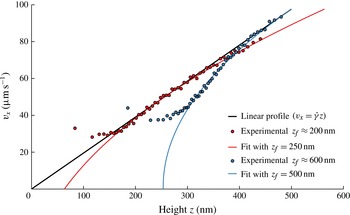
Appendix A. Experiments dedicated to checking the analysis of the defocusing effect
Experiments showing the velocity profiles obtained at different positions of the TIRF objective, thus at different
 $z_{f}$
. Red dots are obtained for
 $z_{f}\approx 200~\text{nm}$
and blue dots correspond to
 $z_{f}\approx 600~\text{nm}$
. Full lines show good agreement between experimental data and (A 1) within a range of altitudes where it is expected to apply, for the depth of field
 $a=348~\text{nm}$
of the objective.

In order to support the theoretical analysis of the effect of defocusing made in § 4, we carried out dedicated experiments. We moved the position of the focal plane
 $z_{f}$
by translating the TIRF objective with a piezo actuator (P-721 PIFOC nanopositioner controlled by E-662 LVPZT servo-amplifier, PI). At each position, we determined velocity profiles. Here, red and blue dots represent experimental data obtained with a 40 wt% sucrose solution for an hydrophilic wall, for two different
 $z_{f}$
,
 $200\pm 50$
and
 $600\pm 50~\text{nm}$
. The results are fitted with an expression derived from (4.7):
 $$\begin{eqnarray}V_{x}(z_{app})=\dot{{\it\gamma}}\left[z_{app}-p\log \left(1+\left(\frac{z_{app}-z_{f}}{P_{c}}\right)^{2}\right)\right]\end{eqnarray}$$
which captures the essence of the theoretical description made in § 4. As shown in figure 13, we found that formula (A 1) captures well the effect, within a range of altitudes where it is expected to apply, i.e. outside the Debye layer. These experiments provided an experimental check of the theoretical description of the defocusing effect made in § 4.
In practice, we tuned
 $z_{f}$
between 200 and 360 nm in our Langevin model so as to minimize the curvature observed at long distances on the velocity profiles. The interval of
 $z_{f}$
that is chosen is justified by the experimental procedure we took, which consists of adjusting the position of the objective to obtain a number of bright particles well in focus. Owing to the existence of a depletion in the Debye layer, the particles we focus on with this procedure are located, typically, between 200 and 400 nm from the wall.