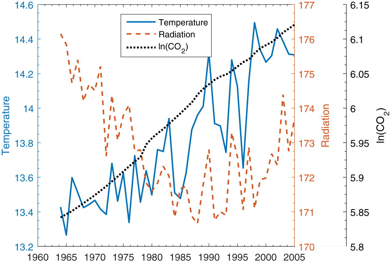
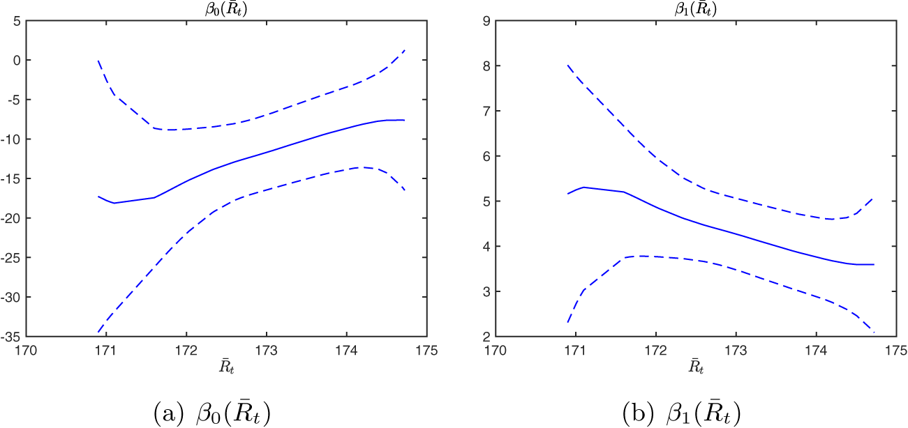
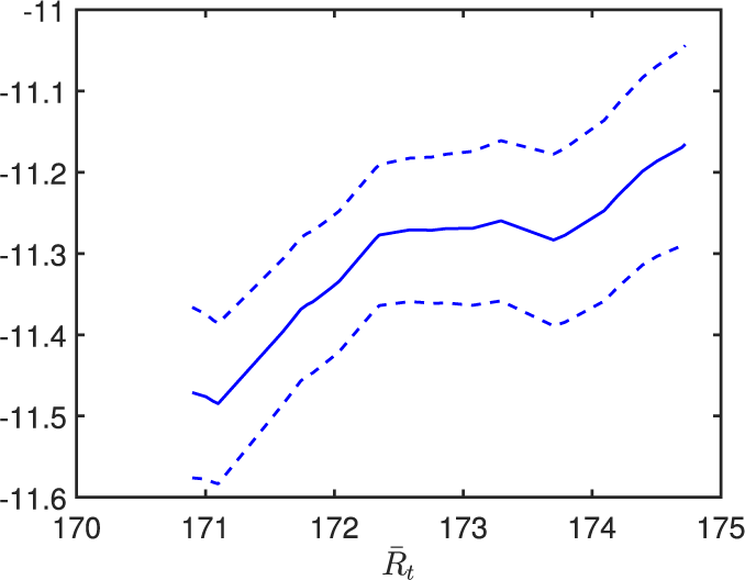
1 INTRODUCTION
In time-series econometrics, a key element in the asymptotics for nonstationary regression was the development of limit theory for the sample moments and cross moments of nonstationary processes. This development was largely completed by the mid 1990s enabling a full understanding of estimation and testing in linear regression with integrated and fractionally integrated time series, covering both cointegrated and spurious model specifications. A much wider class of econometric applications involves nonparametric and semiparametric regressions. But these models present more substantial difficulties in the development of asymptotic theory. Early foundational research addressing some of these complexities appeared in Park and Phillips (Reference Park and Phillips1999, Reference Park and Phillips2000, Reference Park and Phillips2001), Karlsen and Tjøstheim (Reference Karlsen and Tjøstheim2001), and Pötscher (Reference Pötscher2004); and later work on nonparametric cointegrated regression includes Wang and Phillips (Reference Wang and Phillips2009a; hereafter, Reference Wang and PhillipsWP2009a), Wang and Phillips (Reference Wang and Phillips2009b; hereafter, Reference Wang and PhillipsWP2009b), Wang and Phillips (Reference Wang and Phillips2016), Phillips (Reference Phillips2009), Phillips, Li, and Gao (Reference Phillips, Li and Gao2017), and Wang, Phillips, and Kasparis (Reference Wang, Phillips and Kasparis2021).
To encompass a wide class of econometric applications, a long desired and necessary objective in the development of nonparametric regression asymptotics is a general local limit theory for statistics that take the following sample cross moment form:
 $$ \begin{align} &S_n = \frac {c_n}n\sum_{k=1}^n g(Y_{nk}) f( c_nX_{nk}) , \end{align} $$
involving two nonstationary standardized arrays
 $X_{nk}$
and
 $Y_{nk}$
, a continuous function
 $g(\cdot ),$
and a function
 $f(\cdot )$
that includes kernels of the type commonly used in nonparametrics. Sample moments, such as (1.1), play a central role in a large proportion of econometric estimation and inference. An important aspect of the generality in (1.1) is the presence of two numerical sequences: a sample size
 $n \to \infty $
and a bandwidth-related sequence
 $c_n \to \infty $
for which
 $c_n/n\to 0$
. These features are essential for full asymptotic analysis of the sample covariance functional in (1.1). The arrays
 $X_{nk}$
and
 $Y_{nk}$
that appear in this functional are suitably standardized time series for which the weak convergence
 $$ \begin{align} \big(Y_{n,[nt]}, X_{n,[nt]}\big) \Rightarrow (Y_t, X_t) \end{align} $$
holds in the Skorokhod space
 $D_{{\mathbb R}^{2}}[0,1]$
.
Asymptotic theory of
 $S_n$
in this general form was first considered in Phillips (Reference Phillips2009), where the theory essentially required independence between the time series
 $X_{nk}$
and
 $Y_{nk}$
, so there was no linkage between the variables. That work was primarily relevant to the study of spurious nonparametric regression and the analysis therein extended earlier work on linear spurious regression (Phillips, Reference Phillips1986), showing that all of the main asymptotic features of spurious regression coefficients, tests, and diagnostics carried over to the nonparametric case upon adjustment of convergence and divergence rates to take account of the nonparametric nature of the regression. In more recent work, Wang et al. (Reference Wang, Phillips and Kasparis2021) investigated the asymptotics of
 $S_n$
allowing for an explicit linkage between the variables. Their work considered the situation where
 $X_{nk}$
is close to being linearly cointegrated with
 $Y_{nk}$
with an asymptotically constant coefficient and a stationary shift subject to an asymptotically negligible error.
The present article contributes to this past body of research by providing a general framework that encompasses all these models as well as various new models and intermediate formulations, thereby providing a unified theory for use in econometric work involving nonparametric regressions of many different types. Our analysis here assumes that both
 $X_{nk}$
and
 $Y_{nk}$
are scalar. Use of scalar
 $X_{nk}$
is required for technical reasons that are discussed in
Reference Wang and PhillipsWP2009a
, but extensions to vector
 $Y_{nk}$
follow directly and are therefore not detailed. Further, in addition to (1.1), limit distribution theory in nonparametric regression typically also requires treatment of sample covariance statistics of the form
 $$ \begin{align} M_{n} =& \Big(\frac {c_n}n\Big)^{1/2}\sum_{k=1}^n g(Y_{nk}) f( c_nX_{nk}) \, u_k, \end{align} $$
where, with respect to an appropriate filtration
 $\{{\cal F}_k\}_{k\ge 1}$
,
 $\mathbb E(u_k| {\cal F}_{k-1})=0$
so that
 $M_{n}$
is closely related to a martingale sequence, as discussed in detail in Section 2. The asymptotics for (1.3) are straightforward using Wang’s (Reference Wang2014) extended martingale central limit theorem once the asymptotic theory and weak convergence of
 $S_{n}$
itself are established. The important element in that limit theorem is its use of weak convergence rather than convergence in probability of the sample moment (1.1). A limit distribution theory for more general versions of
 $M_n$
that are useful in practical work is given in Theorem 3.2 below. Some regression model implementations of that theory that reveal its generality are given in Section 4.
With results for the covariance functionals (1.1) and (1.3) in hand, the limit theory for nonparametric and semiparametric regression statistics follows in a straightforward manner, as shown later in the article. The limit theory also applies to spurious nonparametric regression, extending Phillips (Reference Phillips2009), and various semiparametric functional coefficient models for time series (Gao and Phillips, Reference Gao and Phillips2013; Sun, Cai, and Li, Reference Sun, Cai and Li2013; Tu and Wang, Reference Tu and Wang2022; Phillips and Wang, Reference Phillips and Wang2023) and panel regressions (Phillips and Wang, Reference Phillips and Wang2022). In particular, our methods apply to nonlinear cointegrating regressions in which the cointegrating coefficients are allowed to depend on covariates that may themselves be nonstationary. Such models are particularly useful in climate science applications of the type studied later in this article.
The remainder of the article proceeds as follows. Assumptions and preliminary results are given in Section 2. Section 3 gives the main results. Sections 4–6 provide regression applications, simulations, and empirics.Footnote
1
Our climate data application is, to the best of our knowledge, the first nonparametric empirical analysis to assess potential nonlinear impacts of CO
 $_2$
on Earth’s climate sensitivity, allowing for nonstationarity in the regressors and the covariates that influence the coefficient responses to the regressors. Section 7 concludes. Proofs are given in Section 8 and Section 9 describes the bootstrap procedure employed in Section 5.
Throughout the article, we use conventional notation except where explicitly mentioned. For
 $x=(x_{ij})_{1\le i\le m, 1\le j\le k}, ||x||=\sum _{i=1}^m\sum _{j=1}^k|x_{ij}|$
.
 $(n, K)_{\textrm {seq}} \to \infty $
denotes that
 $n\to \infty $
followed by
 $K\to \infty $
.
 $A^{\mathrm T}$
denotes the transpose of a vector or matrix A and
 $\mathbb {I}$
is an identity matrix. We denote constants by
 $C, C_1,\ldots $
, which may differ at each appearance.
2 ASSUMPTIONS AND PRELIMINARIES
Let
 $\epsilon _j, j\in \mathbb {Z}$
, be a sequence of iid random variables with
 $\mathbb {E} \epsilon _{0}=0$
and
 $\mathbb {E}\epsilon _0^2=1$
and
 $\xi _{j}=\sum _{k=0}^{\infty }\,\phi _{k}\,\epsilon _{j-k},j\geq 1,$
be a linear process whose coefficients
 $\phi _{k},k\geq 0$
, satisfy one of the following (long memory or short memory) conditions:
-
LM.
 $\phi _{k}\sim k^{-\mu }\,a(k),$
where
$1/2<\mu <1$
and
$a(k)$
is a function slowly varying at
$\infty $
.
-
SM.
$\sum _{k=0}^{\infty }|\phi _{k}|<\infty $
and
$\phi \equiv \sum _{k=0}^{\infty }\phi _{k}\not =0$
.




Suppose that
 $\lim \sup _{t\to \infty }t^{\delta }|\mathbb {E}e^{it\epsilon _0}|<\infty $
for some
 $\delta>0$
throughout this article. This distributional smooth condition on
 $\epsilon _0$
is required to establish the convergence to local time for a partial sum process of
 $\xi _j$
, as seen in the proof of the main result. To establish asymptotic theory for
 $S_n$
, the following assumptions on
 $X_{nk}$
and
 $Y_{nk} $
are employed:
-
A1
$X_{nk}=x_k/d_n$
, where
$x_k=\rho _n x_{k-1}+\xi _k$
with
$\rho _n=1-\tau n^{-1}$
for some
$\tau \ge 0$
,
$x_{0}=o_P(\sqrt n)$
and
$d_n^2=\mathbb {E}\big (\sum _{k=1}^{n}\xi _{k}\big )^{2}$
; -
A2
$Y_{nk}=y_k/d_{yn}$
, where
$d_{yn}^2=var(y_n)\to \infty $
and, on
$D_{{\mathbb R}^3}[0,1]$
,
$$ \begin{align*} \left( \frac{1}{\sqrt{n}} \sum_{i=1}^{\lfloor nt\rfloor }\epsilon _{-i},\ \frac{1 }{\sqrt{n}}\sum_{i=1}^{\lfloor nt\rfloor }\epsilon _{i},\ Y_{n, \lfloor nt \rfloor}\right) &\Rightarrow\big( B_{-t},\ B_{t}, \ Y_{t}\big), \end{align*} $$
where
$\{Y_t\}_{t\ge 0}$
is a path continuous Gaussian process,
$\{B_{t}\}_{t\ge 0}$
is a standard Brownian motion, and
$\{B_{-t}\}_{t\ge 0}$
is an independent copy of
$\{B_t\}_{t\ge 0}$
.


A1 allows for the nearly integrated process
 $x_k$
to be generated either from short memory (under SM) or long memory (under LM) innovations, giving a general framework for practical work. It is well-known that
 $$ \begin{align} d_{n}^{2} =&\mathbb{E}|\sum_{k=1}^{n}\xi_{k}|^{2}\ \sim\ \left \{\begin{array}{@{}ll@{}} c_{\mu }\,n^{3-2\mu }a^{2}(n), & \text{under }\textbf{LM}, \\ \phi^2\, n, & \text{under }\textbf{SM}, \end{array} \right. \end{align} $$
where
 $c_{\mu }$
is a constant (see, e.g., Wang, Lin, and Gulati, Reference Wang, Lin and Gulati2003). A2 is a minor requirement on
 $Y_{nk}$
and the innovations
 $\epsilon _k$
that generate
 $X_{nk}$
, which is close to being necessary for the derivation of asymptotics of
 $S_n$
when
 $X_{nk}$
has a linear structure of the type given in A1. No restrictions are imposed between the limit processes
 $Y_t$
and
 $B_t$
(
 $B_{-t}$
), indicating that many types of potential linkages between
 $X_{nk}$
and
 $Y_{nk}$
are allowed so that
 $Y_{nk}$
has a similar structure to
 $X_{nk}$
. For an explicit example of A2 that is advantageous in applications, we write
 $\eta _j=(\eta _{j1}, \ldots , \eta _{jd})^{\mathrm T}$
and assume that
 $\lambda _j =(\epsilon _j, \eta _j^{\mathrm T}), j\in \mathbb {Z}$
, is a sequence of iid random vectors on
 ${\mathbb R}\times {\mathbb R}^d$
for some integer
 $d\ge 1$
with
 $\mathbb {E} \lambda _{0}=0$
and
 $\mathbb {E}||\lambda _0||^2<\infty $
. Then, consider the following assumption for
 $Y_{nk}$
:
-
A2′
$Y_{nk}=y_k/d_{yn}$
with
$d_{yn}^2=var(y_n)$
, where
$y_k=\sum _{s=1}^k\alpha ^{\mathrm T}v_s$
,
$\alpha =(\alpha _1,\alpha _2,\ldots ,\alpha _{p})^{\mathrm T}\in {\mathbb R}^{p}$
, and
$v_s=(v_{s1},\ldots ,v_{s p})^{\mathrm T}$
is a linear p-vector process with
$p \le d$
satisfying the following conditions:-
(i)
$v_{s}=\sum _{j=0}^{\infty }\Psi _{j}\,\eta _{s-j} $
with
$p \times d$
coefficient matrices
$\Psi _{j}$
satisfying
$\sum _{j=0}^{\infty }j^{1/2}||\Psi _{j}||<\infty $
with matrix norm
$||\cdot ||$
and
$\Psi :=\sum _{j=0}^{\infty }\Psi _j$
of full rank p; -
(ii)
$\Omega :=\mathbb {E}\big (\eta _1\eta _1^{\mathrm T}\big ) $
is a positive-definite matrix.
-





As shown in the following proposition, A2 can be replaced by A2′
. The structure of
 $y_k$
in A2′
allows for a wide combination of multivariate linear processes, which are used in Section 4 for the regression application.
Proposition 2.1. Under A2′
, on
 $D_{{\mathbb R}^3}[0,1]$
, we have
 $var(y_n)/n\to \,\Gamma :=\alpha ^{\mathrm T} \Psi \,\Omega \Psi ^{\mathrm T}\alpha $
and
 $$ \begin{align} \left( \frac{1}{\sqrt{n}} \sum_{i=1}^{\lfloor nt\rfloor }\epsilon _{-i},\ \frac{1 }{\sqrt{n}}\sum_{i=1}^{\lfloor nt\rfloor }\epsilon _{i},\ Y_{n, \lfloor nt \rfloor}\right) \Rightarrow& \big( B_{-t},\ B_{t}, \ Y_t\big) \end{align} $$
with
 $Y_t=\Gamma ^{-1/2}\, \alpha ^{\mathrm T} \Psi \, \Lambda _t$
, where
 $Z_t:=(B_{-t}, B_t, \Lambda _t)$
is a
 $(2+d)$
-dimensional continuous Gaussian process with mean zero, independent increments, and covariance matrix:
 $$ \begin{align*}\Omega_t=t\, \left(\begin{matrix}1& 0 &0\\ 0&1& \gamma^{\mathrm T}\\ 0&\gamma&\Omega\end{matrix}\right)\quad \text{with }\gamma=(\gamma_1,\ldots,\gamma_d)^{\mathrm T} \text{ and } \gamma_k=E(\epsilon_0\eta_{0k}).\end{align*} $$
We further mention that A2, together with standard functional limit theory (see Buchmann and Chan, Reference Buchmann and Chan2007 or Theorem 2.21 of Wang, Reference Wang2015 with a minor modification), implies the joint convergence
 $$ \begin{align} \left( \frac{1 }{\sqrt{n}}\sum_{i=1}^{\lfloor nt\rfloor }\epsilon _{-i},\ \frac{1}{\sqrt{n}} \sum_{i=1}^{\lfloor nt\rfloor }\epsilon _{i}, \ X_{n, \lfloor nt\rfloor}, \ Y_{n, \lfloor nt\rfloor}\right) \Rightarrow& \big( B_{-t}, \ B_{t}, \ X_t, \ Y_t\big), \end{align} $$
on
 $D_{\mathbb {R}^{4}}[0,1]$
, where
 $X_t$
is defined by
 $$ \begin{align} X_t =&\widetilde F(t)+\tau\int_0^te^{-\tau(t-s)}\widetilde F(s)ds, \end{align} $$
with
 $\widetilde F(t) =\left \{\begin {array} {@{}ll} F_{3/2-\mu }(t), & \text {under }\textbf {LM},\\ F_{1/2}(t), & \text {under }\textbf {SM}, \end {array}\right .$
where
 $F_H(t)$
is a fractional Brownian motion with representation
 $$ \begin{align*} F_{H}(t) =& \kappa_H\, \int_{-\infty}^t \big[(t-u)_{+}^{H-1/2}-(-u)_+^{H-1/2}\big]\, dB_u, \end{align*} $$
where we use the notation
 $a_+=\max \{a, 0\}$
and
 $\kappa _H$
is a standardizing constant so that
 $\mathbb {E}F_H^2(1)=~1$
.
We next introduce the regularity conditions on
 $g(x), f(x),$
and
 $u_k$
that are required for the asymptotics of
 $S_n$
and
 $M_n$
.
-
A3
-
(i)
$g(x)$
is a continuous function on
${\mathbb R}$
. -
(ii)
$f(x)$
is a real function on
${\mathbb R}$
satisfying
$\int _{-\infty }^\infty \big (|f(x)|+f^2(x)\big )dx<\infty $
.
-
-
A4
$\{u_k, {\cal F}_k\}_{k\ge 1}$
forms a martingale difference with
$\sigma _k^2=\mathbb {E} \big (u_k^2\mid {\cal F}_{k-1}\big )\to _{a.s.}\sigma ^2>0$
as
$k\to \infty $
, and
$\sup _{k\ge 1}\mathbb {E} \big [|u_k|^{2}I(|u_k|\ge K)\mid {\cal F}_{k-1}\big ]<\infty $
, as
$K\to \infty $
, where is a
$$ \begin{align*} {\cal F}_k=\sigma(u_k, u_{k-1},\ldots; (x_{k+1}, y_{k+1}), (x_k, y_k), \ldots) \end{align*} $$
$\sigma $
-field so that
$x_k$
and
$y_k$
are adapted to
${\cal F}_{k-1}$
.


A3 (ii) is quite weak and close to being necessary for the asymptotic theory of
 $S_n$
and
 $M_{n}$
given in the next section, which was originally used in Reference Wang and PhillipsWP2009a in the case where
 $g(x)= 1$
. A4 ensures that
 $M_{n}=M_{nn}$
, where
 $M_{nk}=\Big (\frac {c_n}n\Big )^{1/2}\sum _{j=1}^k g(Y_{nj}) f( c_nX_{nj}) \, u_j, k\ge 1,$
is a martingale with respect to the natural filtration
 ${\cal F}=\{{\cal F}_k\}_{k\ge 1}$
, which is standard in the literature. When the
 $y_k$
given in A2′
is used in
 $M_n$
, we may take
 ${\cal F}_k=\sigma (u_k, u_{k-1},\ldots; \lambda _{k+1}, \lambda _{k}, \ldots )$
. It should be mentioned that A4 essentially assumes that
 $\sigma _k^2=\mathbb {E} \big (u_k^2\mid {\cal F}_{k-1}\big )$
is asymptotically constant, which is convenient for the development of our main results. Note that
 $ M_n =\Big (\frac {c_n}n\Big )^{1/2}\sum _{k=1}^n g(Y_{nk}) f( c_nX_{nk}) \, \sigma _k \,\hat u_k, $
where
 $\hat u_k=\sigma _k^{-1} u_k$
satisfies that
 $\mathbb {E} \big (\hat u_k^2\mid {\cal F}_{k-1}\big )=1$
. In regression applications, when
 $\sigma _k^2$
does not converge to a constant, we only need to replace the asymptotics of
 $S_n=\frac {c_n}n\sum _{k=1}^n g(Y_{nk}) f( c_nX_{nk}) $
by that of
 $S_{1n}= \frac {c_n}n\sum _{k=1}^n g(Y_{nk}) f( c_nX_{nk}) \sigma _k$
, as is similarly considered in Corollary 3.1 below. We remark that the conditional variances
 $\sigma _k$
are generally unknown and must be estimated (by
 $\widehat \sigma _k$
, say), which then requires corresponding asymptotics of the statistic
 $\widehat S_{1n} =\frac {c_n}n\sum _{k=1}^n g(Y_{nk}) f( c_nX_{nk}) \widehat \sigma _k$
. If
 $\widehat \sigma _k$
is suitably chosen so that
 $\widehat \sigma _k\in {\cal F}_{k}$
, then Corollary 3.1 remains useful in establishing asymptotics for
 $\widehat S_{1n}$
. The details are left for future work.
We finally mention that the diffusion
 $X_t$
defined by (2.4) is a fractional Ornstein–Uhlenbeck process having continuous local time
 $L_X(s, x)$
defined by
 $$ \begin{align*} L_X(s,x) =\lim_{\epsilon\to 0}\frac 1{2\epsilon}\int_0^sI(|X_t-x|\le \epsilon)dt, \quad a.s. \end{align*} $$
See Chapter 2.1.1 of Wang (Reference Wang2015), for instance. Since
 $L_X(s, x)$
is positive and increasing with respect to s, when
 $g(x)$
is a continuous function (i.e., A3 (i) holds),
 $g(Y_s)$
is a continuous process and the following integral (Lebesgue–Stieltjes) exists:
 $$ \begin{align} S(x):= \int_0^1 g(Y_s) L_X(d s, x). \end{align} $$
Moreover, from the continuity of
 $L_X(t, x)$
,
 $S(x)$
is continuous and bounded almost surely. Hence, by dominated convergence for any
 $a(x)$
satisfying
 $\int _{-\infty }^\infty |a(x)| dx<\infty $
, we have
 $$ \begin{align} \lim_{\epsilon\to 0}\, \int_{-\infty}^\infty a(x)\, S(\epsilon\, x) dx =& S(0)\, \int_{-\infty}^\infty a(x) dx, \quad a.s. \end{align} $$
The random integral
 $S(x)$
is involved in the limit distributions of
 $S_n$
and
 $M_{n}$
, and (2.6) will be used in proofs of the main results without further indication.
3 MAIN RESULTS
We start with the following theorem and some extensions, which are subsequently used in the asymptotic analysis of sample covariance statistics that are useful in applications.
Theorem 3.1. Suppose A1–A3 hold. Then, for any
 $c_n\to \infty $
and
 $c_n/n\to 0$
, we have
 $$ \begin{align} S_n = \frac {c_n}n\sum_{k=1}^n g(Y_{nk}) f( c_nX_{nk} ) \rightarrow_D& \ \mathbb{S}=\, S(0)\, \int_{-\infty}^\infty f(x) dx, \end{align} $$
and the following joint convergence also holds: on
 $D_{\mathbb {R}^{5}}[0,1]$
,
 $$ \begin{align} \left( \frac{1 }{\sqrt{n}}\sum_{i=1}^{\lfloor nt\rfloor }\epsilon _{i},\ \frac{1}{\sqrt{n}} \sum_{i=1}^{\lfloor nt\rfloor }\epsilon _{-i},\ X_{n, [nt]}, \ Y_{n, [nt]},\ S_n\right) \Rightarrow& \big( B_{t},\ B_{-t},\ X_t, \ Y_t,\ \mathbb{S}\big). \end{align} $$
Remark 3.1. When
 $g(x)= 1$
, Theorem 3.1 reduces to Theorem 2.1 of Reference Wang and PhillipsWP2009a. See also Jeganathan (Reference Jeganathan2004). In comparison with the latter papers, our condition on
 $X_{nk}$
is slightly stronger but more direct for practical applications. As is well known in the literature, the condition
 $c_n\to \infty $
is necessary for a limit result such as (3.1). Indeed, if
 $c_n=1$
, the limit distribution of
 $S_n$
is a standard stochastic integral, namely,
 $$ \begin{align} \frac {1}n\sum_{k=1}^n g(Y_{nk}) f( X_{nk} ) \to_D& \int_0^1 g(Y_t) f(X_t) dt \nonumber\\ =&\int_{-\infty}^\infty f(s) \int_0^1 g(Y_t)L_X(dt, s) ds\not = S(0)\, \int_{-\infty}^\infty f(x) dx, \end{align} $$
where we have used the occupation time formula in (3.3). As shown in Reference Wang and PhillipsWP2009a, some simple sequential limit arguments help to reveal the nature of these differences. Start by rewriting the average
 $S_{n}$
so that it is indexed by twin sequences
 $ c_{m}$
and n defining
 $S_{m,n}=\frac {c_{m}}{n}\,\sum _{k=1}^{n}g(Y_{nk})f(c_{m} \,X_{nk})$
and noting that
 $S_{m,n}=S_{n}$
when
 $m=n.$
If we hold
 $c_{m}$
fixed as
 $n\rightarrow \infty ,$
then standard limit theory leads to the following limit behavior:
 $$ \begin{align} S_{m,n} \rightarrow _{D}&c_{m}\int_{-\infty}^\infty f(c_{m}x) \int_0^1 g(Y_t)L_X(dt, x) dx\notag \\ =&\int_{-\infty}^\infty f(x) \int_0^1 g(Y_t)L_X(dt, x/c_m) dx :=S_{m,\infty }. \end{align} $$
It follows from (2.6) with
 $a(x)=f(x)$
that
 $S_{m,\infty }\rightarrow _{a.s.}S(0)\, \int _{-\infty }^\infty f(x) dx$
when
 $c_m \to \infty $
as
 $m\rightarrow \infty ,$
so that (3.1) may be regarded as a limiting version of (3.4). The goal and the technical difficulty are to turn this sequential argument as
 $n\rightarrow \infty ,$
followed by
 $m\rightarrow \infty ,$
into a joint limit argument so that
 $c_{n}$
may play an active role as a bandwidth parameter in density estimation and kernel regression.
Remark 3.2. The key approach in the proof of Theorem 3.1 depends on the convergence of the following difference:
 $$ \begin{align*} \Delta_n(\epsilon)&:= S_n- \frac {c_n}{n}\,\sum_{k=1}^ng(Y_{nk}) \int_{-\infty}^{\infty} f\big[ c_n\,( X_{nk}+z\epsilon)\big] \phi(z)dz\\ &=\frac {c_n}{n}\,\sum_{k=1}^ng(Y_{nk}) \int_{-\infty}^{\infty}\big\{ f\big( c_n\, X_{nk}\big)-f\big[ c_n\,( X_{nk}+z\epsilon)\big]\big\}\phi(z)dz, \end{align*} $$
as
 $n\to \infty $
followed by
 $\epsilon \to 0$
, where
 $\phi (z)=\frac 1{\sqrt {2\pi }}e^{-z^2/2}$
. When
 $g(x)=1$
,
 $\Delta _n(\epsilon )\to _{\mathbb P} 0$
was established in Jeganathan (Reference Jeganathan2004) and later by Reference Wang and PhillipsWP2009a under weak conditions. That result with
 $g(x)=1$
cannot be directly used when
 $g(x)\not =1$
due to the involvement of
 $Y_{nk}.$
However, in view of the tightness of
 $\{Y_{n,[nt]}\}_{ 0\le t\le 1}$
and the continuity of
 $g(x)$
, there exists
 $m=m_{n, \epsilon }\to \infty $
as
 $n\to \infty $
followed by
 $\epsilon \to 0$
so that
 $$ \begin{align*} \max_{1\le j\le n/m} \hspace{1mm} \max_{(j-1)m+1\le k\le jm} |g(Y_{nk})-g(Y_{n,(j-1)m+1})|=o_P(1). \end{align*} $$
In consequence, letting
 $T_n=[n/m]$
, the difference
 $\Delta _n(\epsilon )$
can be approximated by the following blocked sequence:
 $$ \begin{align*} \Delta_{n1}(\epsilon)=&\frac {c_n}{n}\,\sum_{j=2}^{T_n} g(Y_{n,(j-1)m+1}) \sum_{k=(j-1)m+1}^{jm} \int_{-\infty}^{\infty} \kern-1.2pt\big\{ f\big( c_n\, X_{nk}\big)-f\big[ c_n\,( X_{nk}+z\epsilon)\kern-1pt\big]\kern-0.5pt\big\}\phi(z)dz. \end{align*} $$
When
 $g(x)$
is bounded, by similar arguments (differing only in details) as those in Reference Wang and PhillipsWP2009a, we have
 $$ \begin{align*} |\Delta_{n1}(\epsilon)|\le &\frac {C\, c_n}{n}\,\sum_{j=2}^{T_n} \, \Big|\, \sum_{k=(j-1)m+1}^{jm} \int_{-\infty}^{\infty} \big\{ f\big( c_n\, X_{nk}\big)-f\big[ c_n\,( X_{nk}+z\epsilon)\big]\big\}\phi(z)dz \,\Big| \to_P 0, \end{align*} $$
as
 $n\to \infty $
followed by
 $\epsilon \to 0$
, Hence,
 $\Delta _n(\epsilon ) \to _P 0$
is established by means of the convergence
 $\Delta _{n1}(\epsilon )\to _P 0$
, since the boundedness of
 $g(x)$
can be removed by standard truncation methods as shown in the final part of the proof of Theorem 3.1.
Theorem 3.1 may be extended by allowing
 $S_n$
to include certain stationary variables. Indeed, if we define
 $\lambda _k=(\epsilon _k, \eta _{k1}, \ldots ,\eta _{kd})$
as in Section 2, i.e.,
 $\lambda _k, k\in {\cal Z},$
is a sequence of iid random vectors on
 ${\mathbb R}\times {\mathbb R}^d$
for some integer
 $d\ge 1$
, and set
 $$ \begin{align*} S_{1 n} =& \frac{c_{n}}{n}\, \sum_{k=1}^{n}g(Y_{nk}) f_1(c_n\,X_{nk}, \lambda_k, \dots, \lambda _{k-m}), \end{align*} $$
where
 $m\ge 0$
is an integer and
 $f_1(\cdot ,\cdot )$
is a real-valued function that is well defined in each of its arguments, we have the following corollary.
Corollary 3.1. Suppose A1, A2, and A3(i) hold. Suppose that:
-
A5.
-
(i) for any
$x\in {\mathbb R}$
and
$y\in {\mathbb R}^{(m+1)d+1}$
and for some
$\beta>0$
,
$ |f_1(x, y)|\le T(x)(1+||y||^\beta ), $
where
$T(x)$
is a bounded and integrable function; -
(ii)
$E||\lambda _{0}||^{2\wedge (2\beta )}<\infty $
.
-


Then, for any
 $c_n\to \infty $
satisfying
 $c_n/n\to 0$
, we have
 $$ \begin{align} &\left(\frac {1}{\sqrt n}\sum_{k=1}^{[nt]}\epsilon_k, \ \frac {1}{\sqrt n}\sum_{k=1}^{[nt]}\epsilon_{-k},\ X_{n, [nt]},\ Y_{n, [nt]},\ S_{1n}\,\right) \nonumber\\ &\Rightarrow\ \Big(B_t,\ B_{-t},\ X_t,\ Y_t, \ {\mathbb{S}_1} \Big) \, \end{align} $$
on
 $D_{{\mathbb R}^5}[0, 1]$
, where
 $ {\mathbb {S}_1}= S(0)\, \int _{-\infty }^\infty \tilde f_{1}(x)dx $
with
 $\tilde f_{1}(x)=\mathbb {E} f_1(x, \lambda _m,\ldots ,\lambda _0)$
.
Remark 3.3. The proof of Corollary 3.1 involves demonstrating negligibility of the residual difference
 $$ \begin{align*} R_{n}=& \frac{c_{n}}{n}\, \sum_{k=1}^{n}g(Y_{nk}) \big[f_1\big(c_n\,X_{nk},\lambda_k, \ldots, \lambda _{k-m}) -\tilde f_1(c_n\,X_{nk})\big]. \end{align*} $$
Using similar ideas, a further extension of this result is possible, along the lines of Theorem 4.1 in Wang et al. (Reference Wang, Phillips and Kasparis2021), where
 $f_1(c_n\,X_{nk}, \lambda _k, \ldots , \lambda _{k-m})$
in (3.5) is replaced by
 $f_1(c_n\,X_{nk}, \tilde \lambda _k)$
in which
 $\tilde \lambda _k$
is a linear process with innovations
 $\lambda _k$
and
 $f_1(x, y)$
satisfies certain smoothness conditions. This extension only involves some additional calculations rather than new ideas, so the details are omitted. Statistics, such as
 $S_{1n}$
, appear in nonlinear cointegrating regression with additional stationary regressors. An example is given in Wang et al. (Reference Wang, Phillips and Kasparis2021).
Remark 3.4. An earlier sequence of papers (Wang and Phillips, Reference Wang and Phillips2009a, Reference Wang and Phillips2009b, Reference Wang and Phillips2024) developed asymptotics of sample covariances, such as
 $(n/c_n)^{1/2}S_n$
or
 $(n/c_n)^{1/2}S_{1n}$
when
 $g(x)=1$
in the “zero energy” case where
 $\int _{-\infty }^\infty f(x)dx=0$
or
 $\int _{-\infty }^\infty \tilde f_{1}(x)dx=0$
. The proofs in those papers are technical and involve considerable care in the use of the zero energy nature of the functions. However, in the proof of Theorem 3.1 (and similarly for Corollary 3.1), the key idea is a block decomposition of the form as outlined in Remark 3.2 (also see (8.11) in the proof), where the estimation of a particular remainder term (e.g.,
 $S_{1, n\epsilon }$
in the proof) depends on values of
 $|f(X_{nk})|$
rather than
 $f(X_{nk})$
due to the involvement of the nonstationary time series
 $Y_{nk}$
, so that the advantages of a zero energy condition in obtaining sharp results are lost. Except for some special situations (e.g., where a martingale structure is imposed) as shown in Theorem 3.2 below, it is unclear at present how to bridge across these different techniques to achieve a completely general analysis of the zero energy case. So this task is left for future work.
3.1 Asymptotics for Sample Covariance Statistics
Regression applications often require limit theory for sample covariance statistics
 $M_n$
defined by (1.3) and
 $M_{1n}$
of the following form:
 $$ \begin{align*} M_{1n} =& \Big(\frac{c_{n}}{n}\Big)^{1/2}\sum_{k=1}^{n}g(Y_{nk}) f_1\big[c_n\,(X_{nk}+c_n' x), \lambda_k, \ldots, \lambda _{k-m}\big] \, u_k, \end{align*} $$
where x is fixed and the constant sequence
 $c_n'\to 0$
or
 $c_n'=1$
. Using Theorem 3.1 and Corollary 3.1, together with the extended martingale limit theorem given in Wang (Reference Wang2014), we obtain the second main result.
Theorem 3.2. If A1, A2′, A3(i), and A4 hold, and if
 $f(x)$
is a bounded integrable real function, then
 $$ \begin{align} \big( \widetilde S_{n}, \ M_{n}\big) \to_D& \big(\widetilde{\mathbb{S}}, \ \sigma\,\widetilde {\mathbb{S}}^{1/2} \, \mathbb{N}\big), \, \end{align} $$
for any
 $c_n\to \infty $
and
 $c_n/n\to 0$
, where
 $$ \begin{align*} \widetilde S_{n} = \frac {c_n}n\,\sum_{k=1}^n g^2(Y_{nk}) f^2\big( c_nX_{nk} \big), \quad \widetilde {\mathbb{S}}= \int_0^1 g^2(Y_s) L_X(d s, 0)\, \int_{-\infty}^\infty f^2(x)dx \end{align*} $$
and
 $\mathbb {N}$
is a standard normal variate independent of
 $X=\{X_t\}_{t\ge 0}$
and
 $Y=\{Y_t\}_{t\ge 0}$
.
Similarly, if in addition to A1, A2′
, A3(i), A4, and A5(i),
 $E||\lambda _{0}||^{4\beta +2}<\infty $
, and
 $f_1(x)$
is a bounded integrable real function, then
 $$ \begin{align} \big( \widetilde S_{1n}, \ M_{1n}\big) \to_D& \big(\widetilde{\mathbb{S}_1}, \ \sigma\, \widetilde {\mathbb{S}}_1^{1/2} \, \mathbb{N}\big), \, \end{align} $$
for any
 $c_n\to \infty $
and
 $c_n/n\to 0$
, where
 $$ \begin{align*} \widetilde S_{1n} =& \frac {c_n}n\,\sum_{k=1}^n g^2(Y_{nk}) f^2_1\big[ c_n(X_{nk}+c_n'x), \lambda_k, \ldots, \lambda _{k-m}\big] , \end{align*} $$
and
 $$ \begin{align*} \widetilde {\mathbb{S}}_1= \int_0^1 g^2(Y_s) L_X(d s, x')\, \int_{-\infty}^\infty \mathbb{E} f_1^2(x, \lambda_m,\ldots,\lambda_0)dx, \; \textrm{with } x'=\left\{ \begin{array}{@{}ll@{}} 0, & \text{if }c_n'\to 0 \\ -x, & \text{if }c_n'=1. \end{array} \right. \end{align*} $$
Remark 3.5. Under the conditions of Theorem 3.2, if we let
 $M_{n}=M_{nn}$
and
 $M_{1n}=M_{1n, n}$
where, for
 $k\ge 1, M_{nk}=\Big (\frac {c_n}n\Big )^{1/2}\sum _{j=1}^k g(Y_{nj}) f( c_nX_{nj}) \, u_j$
and
 $$ \begin{align*} M_{1n, k} =&\Big(\frac{c_{n}}{n}\Big)^{1/2}\sum_{j=1}^{k}g(Y_{nj}) f_1\big[c_n\,(X_{nj}+c_n' x), \lambda_j, \ldots, \lambda _{j-m}\big] \, u_j, \end{align*} $$
both
 $\{M_{nk}\}_{k\ge 1}$
and
 $\{M_{1n, k}\}_{k\ge 1}$
are martingales with respect to the filtration
 ${\cal F}=\{{\cal F}_k\}_{k\ge 1}$
with
 ${\cal F}_k=\sigma (u_k, u_{k-1},\ldots ;\lambda _{k+1}, \lambda _{k}, \ldots )$
. Therefore, Theorem 3.2 may be readily employed in nonparametric or semi-parametric cointegrating regression contexts such as nonparametric predictive regressions, but it seems difficult to extend to the general sample covariance context, at least using presently available techniques. Indeed, even when
 $u_k=\epsilon _k$
so that
 $M_n$
and
 $M_{1n}$
both lead to endogeneity (as in the much simpler framework of Reference Wang and PhillipsWP2009b where
 $g(x)=1$
) it is unclear at present how to establish the limit theory of
 $M_n$
and
 $M_{1n}$
with general
 $g(x)\not =1$
, as explained in Remark 3.3. Further, the class of functions
 $f_1(\cdot , \cdot )$
in A5(i) or
 $f(\cdot )$
in A3 (ii) is restrictive for parametric regression contexts, where the model may require inclusion of regression functions that fail A3(ii) such as
 $f(x)=x^p$
. These limitations indicate that the technical machinery employed in the present article is insufficient for tackling fully general asymptotics in nonlinear cointegration modeling.
Remark 3.6. Theorem 3.2 uses A2
 $^\prime $
to assist in proving asymptotic normality but this condition can be relaxed. For instance, Theorem 3.2 still holds only if
 $y_k$
satisfies A2 with
 $y_k=l(\lambda _k,\lambda _{k-1},\ldots ), $
where
 $l(\dots )$
is a well-defined measurable function of its components. The proof is similar to that of Theorem 3.2 by verifying the condition of Wang’s (Reference Wang2014) extended martingale central limit theorem, and the details are therefore omitted.
4 REGRESSION APPLICATIONS
Nonlinear cointegrating regressions with functional coefficients were introduced in Xiao (Reference Xiao2009) and Cai, Li, and Park (Reference Cai, Li and Park2009), where the authors suggested a model of the form
 $$ \begin{align} z_k=l_k^{\mathrm T}\beta (x_k)+u_{k}, \end{align} $$
where
 $\{x_k, z_k, u_k\}$
are scalars,
 $l_k=(l_{k1},\ldots ,l_{kp})^{\mathrm T}$
is of dimension p to be specified later,
 $\beta (\cdot )=\big (\beta _0(\cdot ), \beta _1(\cdot ),\ldots ,\beta _{p-1}(\cdot )\big )^{\mathrm T}$
is a p-vector of unknown smooth functions
 $\beta _{s}(\cdot ), s=0,1,\ldots , p-1,$
defined on
 $\mathbb R$
, and
 $\{u_k, {\cal F}_k\}_{k\ge 1}$
forms a martingale difference so that
 $E\big ( z_k|{\cal F}_{k-1}\big )=l_k^{\mathrm T}\beta (x_k)$
. Xiao (Reference Xiao2009) dealt with the case where the functional covariate
 $x_k$
in (4.1) is stationary; Cai et al. (Reference Cai, Li and Park2009) restricted the model to cases where either the functional covariate
 $x_k$
in (4.1) or the regressor
 $l_k$
is stationary.
Extensions of the model (4.1) to cases where both
 $x_k$
and
 $l_k$
are nonstationary are considerably more complex but also have many relevant empirical applications, such as the climate sensitivity implementation of our methods in Section 6, where nonstationary regressors and covariates can normally be expected. The required limit theory for these extensions is given in the present section.
Some related versions of the model (4.1) can be found in Gao and Phillips (Reference Gao and Phillips2013), Li et al. (Reference Li, Li, Liang and Hsiao2017), Hirukawa and Sakudo (Reference Hirukawa and Sakudo2018), and Tu and Wang (Reference Tu and Wang2019, Reference Tu and Wang2020). Further recent developments can be found in Tu and Wang (Reference Tu and Wang2022), Phillips and Wang (Reference Phillips and Wang2023), Liang, Shen, and Wang (Reference Liang, Shen, Wang, Chang, Sokbae Lee and Miller2023), and in a panel regression context by Phillips and Wang (Reference Phillips and Wang2022). Phillips and Wang (Reference Phillips and Wang2023) provided a correction to the limit theory in the previous nonstationary kernel regression literature, showing that conventional bias terms can influence both the asymptotic variance and the optimal convergence rate in functional coefficient nonstationary regression.
We develop a general limit theory of estimation and inference in model (4.1) for the local level kernel estimator
 $\widehat {\beta }_n(x)$
of
 $\beta (x)$
defined by
 $$ \begin{align} \widehat{\beta}_n(x) &=\underset{\beta}{\arg\min} \sum^n_{k=1}[z_k-l_k^{\mathrm T}\beta]^2K\Big(\frac{x_k-x}{h}\Big) \notag \\ &=\left[\sum^n_{k=1}l_kl_k^{\mathrm T}K\Big(\frac{x_k-x}{h}\Big)\right]^{-1}\sum^n_{k=1}l_k\, z_k\,K\Big(\frac{x_k-x}{h}\Big), \end{align} $$
where
 $K(x)$
is a nonnegative real kernel function and the bandwidth parameter
 $h\equiv h_{n}\rightarrow 0$
as
 $n\rightarrow \infty $
. The results in Section 3 are used here to accommodate dual nonstationarity where both regressors
 $l_k$
and covariate
 $x_k$
are nonstationary time series. For the same model and improved estimation of
 $\beta (x),$
this section also considers local linear estimation and provides asymptotics under additional restrictions between
 $x_k$
and
 $l_k$
.
To avoid further complexity, except where explicitly mentioned, we employ in what follows the same notation and conditions as in previous sections on
 $x_k, u_k, \lambda _k$
, and
 $v_k$
. Let x be a fixed constant in
 ${\mathbb R}$
and, in a neighborhood of x, consider the following local linear and quadratic conditions on the functional coefficient
 $\beta {(\cdot )}=\big (\beta _0(\cdot ), \beta _1(\cdot ),\ldots ,\beta _{p-1}(\cdot )\big )^{\mathrm T}$
:
-
A6.
-
(i)
$||\beta (y+x)-\beta (x)-\beta '(x)y||\leq C_x\, |y|^{1+\nu }$
, or -
(ii)
$ ||\beta (y+x)-\beta (x)-\beta '(x)y-\frac 12 \beta "(x)y^2||\leq C_x\, |y|^{2+\nu }, $
A6. for some
$0<\nu \le 1$
, where
$C_x$
is a constant depending only on x. -


We also make use of the following condition on the kernel function
 $K(\cdot )$
used in (4.2):
-
A7.
-
(i)
$K(x)$
is a positive real function with finite support satisfying
$\int _{-\infty }^\infty K(s)ds =1$
, or -
(ii)
$K(x)$
is a positive real function with finite support satisfying
$\int _{-\infty }^\infty K(x)dx =1$
and
$\int _{-\infty }^\infty xK(x)dx=0$
.
-


Under these conditions, the next result provides the asymptotic theory of
 $\widehat {\beta }_n(x)$
.
Theorem 4.1. Suppose that A1 and A4 hold. Suppose
 $l_k=\sum _{s=1}^kv_s$
, where
 $v_s=(v_{s1},\ldots v_{sp})^{\mathrm T}, p\le d,$
is a linear vector process as defined as in A2′
, so that
 $l_k$
is full rank
 $I(1)$
. Then, under A6(i) and A7(i), we have
 $$ \begin{align} h^{-1}\, \big[\widehat \beta_n(x)-\beta (x)\big] \to_P& \beta'(x)\, \int_{-\infty}^\infty sK(s) ds, \end{align} $$
for any
 $h\to 0$
satisfying
 $\min \{nh^2, nh/d_n\}\to \infty $
. If A6(i) is replaced by A6(ii), we have
 $$ \begin{align} &\left(\sum_{k=1}^{n} l_kl_k^{\mathrm T} K\big[(x_k-x)/h\big]\right)^{1/2}\,\Big[\hat \beta_n\,(x)- \beta\,(x)- h L_{1n}\,\beta'(x)-\frac 12\, h^2 L_{2n}\,\beta"(x)\Big] \ \nonumber\\ &\to_D\ \sigma_{\beta}\,\mathbb{N}_{p}, \end{align} $$
for any h satisfying
 $n^2h^{5+2\nu }/d_n\to 0$
and
 $nh/d_n\to \infty $
, where, for
 $j=1$
and
 $2$
,
 $$ \begin{align} L_{jn}=& \left\{\sum_{k=1}^{n} l_kl_k^{\mathrm T} K\big[(x_k-x)/h\big]\right\}^{-1}\sum_{k=1}^{n} l_kl_k^{\mathrm T} K_j\big[(x_k-x)/h\big], \quad K_j(s)=s^jK(s), \end{align} $$
 $\sigma _{\beta }^2=\sigma ^2\int _{-\infty }^\infty K^2(x)dx$
and
 $\mathbb {N}_{p} \sim \mathcal {N}(0, {\mathbb I}_{p})$
is a standard p-dimensional normal vector.
Remark 4.1. Result (4.3) shows that, under linear local behavior of
 $\beta (\cdot )$
in conditions A6(i) and A7(i),
 $\widehat \beta _n(x)$
is a consistent estimator of
 $\beta (x)$
when
 $h\to 0$
and, as
 $n \to \infty $
, h satisfies
 $\min \{nh^2, nh/d_n\}\to \infty $
. Observe that in this nonstationary functional regression context, two effective sample size conditions are used to achieve consistency: the first is
 $\sqrt {n}h \to \infty $
for the signal associated with the I(1) regressor
 $l_t$
; and the second is
 $nh/d_n \to \infty $
for the signal associated with the local functional covariate
 $x_t$
.Footnote
2
,Footnote
3
Under local quadratic behavior, in place of the self-normalized limit theory given in (4.4), we also have the (mixed) normal limit theory
 $$ \begin{align} \Big(\frac{n^2h}{d_n}\Big)^{1/2}\,\Big[\hat \beta_n\,(x)- \beta\,(x)- h L_{1n}\,\beta'(x)-\frac 12\, h^2 L_{2n}\,\beta"(x)\Big] \to_D \sigma_{\beta}\, {\cal Y}^{-1/2}\,\mathbb{N}_{p}, \end{align} $$
where
 ${\cal Y}$
is a random matrix independent of
 $\mathbb {N}_{p}$
defined by
 ${\cal Y}=\int _0^1\Psi \, \Lambda _s \Lambda _s^{\mathrm T} \Psi L_X (ds, 0) $
. Here,
 $\Psi \, \Lambda _s$
is as in (2.2) with
 $\Psi $
of full rank and
 $\Lambda _s$
a Gaussian process with positive-definite variance matrix
 $s\Omega $
, from A2′(i) and A2(ii), so that the limiting signal matrix
 ${\cal Y}$
is positive definite almost surely.Footnote
4
Scaling the numerator and denominator of
 $L_{1n}$
and using Proposition 4.1 below gives
 $$ \begin{align*} \frac1{n}\sum_{k=1}^{n} l_kl_k^{\mathrm T} K_1\big[(x_k-x)/h]=O_p[(nh/d_n)^{1/2}], \end{align*} $$
and from Theorem 3.1 with
 $c_n=d_n/h,$
we have
 $$ \begin{align*} \frac{d_n}{hn^2}\sum_{k=1}^{n} l_kl_k^{\mathrm T} K\left[d_n\left(\frac{x_k}{d_n}-\frac{x}{d_n}\right)/h\right]\to_D{\cal Y}. \end{align*} $$
It follows that the asymptotic impact of the
 $O(h)$
bias term on the distribution of
 $\hat \beta _n\,(x)$
is given by
 $$ \begin{align} &\left(\sum_{k=1}^{n} l_kl_k^{\mathrm T} K\big[(x_k-x)/h]\right)^{1/2}hL_{1n}\nonumber\\&\quad =h\left(\sum_{k=1}^{n} l_kl_k^{\mathrm T} K\big[(x_k-x)/h]\right)^{-1/2} \sum_{k=1}^{n} l_kl_k^{\mathrm T} K_1\big[(x_k-x)/h] \notag \\ &\quad= \left(hd_n\right)^{1/2}\left(\frac{d_n}{hn^2}\sum_{k=1}^{n} l_kl_k^{\mathrm T} K\big[(x_k-x)/h]\right)^{-1/2}\frac1{n}\sum_{k=1}^{n} l_kl_k^{\mathrm T} K_1\big[(x_k-x)/h] \notag \\ &\quad=\left(hd_n\right)^{1/2} \times O_p\left(\frac{nh}{d_n}\right)^{1/2} = O_p(\sqrt{n}h), \end{align} $$
which might diverge by virtue of the effective sample size condition
 $\sqrt {n}h \to \infty $
. This indicates that the result (4.4) cannot generally be used in practice for inference.
Remark 4.2. Liang et al. (Reference Liang, Shen, Wang, Chang, Sokbae Lee and Miller2023) investigated the model (4.1) in the case where
 $l_k$
are stationary variables satisfying certain conditions; and Reference Wang and PhillipsWP2009a and Wang and Phillips (Reference Wang and Phillips2011) considered the pure nonparametric regression model in which
 $l_k=1$
. In comparison with (4.4) and (4.6), the results given in Liang et al. (Reference Liang, Shen, Wang, Chang, Sokbae Lee and Miller2023), Reference Wang and PhillipsWP2009a, and Wang and Phillips (Reference Wang and Phillips2011) have the form
 $$ \begin{align*} &\left(\sum_{k=1}^{n} l_kl_k^{\mathrm T} K\big[(x_k-x)/h]\right)^{1/2}\,\left[ \widehat \beta_n(x)-\beta (x) -\frac {h^{2}\beta^{"}(x)}{2}\, \int_{-\infty }^{\infty }s^{2}K(s)ds\right] \to_D\ \sigma_{\beta}\,\mathbb{N}_{p},\\ &\Big(\frac {nh}{d_n}\Big)^{1/2}\,\left[ \widehat \beta_n(x)-\beta (x) -\frac {h^{2}\beta^{"}(x)}{2}\, \int_{-\infty }^{\infty }s^{2}K(s)ds\right] \to_D\ \big[{\mathbb E}(l_1l_1^{\mathrm T}) \big]^{-1}\sigma_{\beta}\,{\cal Y}^{-1/2}\, \mathbb{N}_{p}, \end{align*} $$
i.e., in (4.4) and (4.6), the linear term
 $h L_{1n}\,\beta '(x)$
disappears and
 $L_{2n}$
in the limit theory (4.4) can be replaced by
 $\int _{-\infty }^{\infty }s^{2}K(s)ds$
when
 $l_k$
is stationary. The reason for the difference is that when
 $l_k$
is stationary
 $\sum _{k=1}^{n} l_kl_k^{\mathrm T} K\big [(x_k-x)/h]$
has a reduced signal with divergence rate
 $\frac {nh}{d_n}$
rather than
 $\frac {n^2h}{d_n}$
, so that
 $$ \begin{align*} \Big(\frac{nh}{d_n}\Big)^{1/2}\, h L_{1n}\,\beta'(x) = O_P(h)=o_P(1) \end{align*} $$
and
 $L_{2n}$
can be replaced by
 $\int _{-\infty }^{\infty }s^{2}K(s)ds$
by virtue of a simple calculation. See Liang et al. (Reference Liang, Shen, Wang, Chang, Sokbae Lee and Miller2023) for details. And when
 $l_k$
is nonstationary, Phillips and Wang (Reference Phillips and Wang2023) found explicit limit formulas showing that the bias term can affect both the asymptotic variance and the convergence rates in nonstationary functional coefficient cointegrating regression even when
 $x_k$
is stationary. The present results provide further extension of these findings to the case of multiple nonstationary regressors and a nonstationary functional covariate, both of which are important in practical applications.
We may improve Theorem 4.1 by using local linear estimation (e.g., Fan and Gijbels, Reference Fan and Gijbels1996) and imposing more restrictions between
 $x_k$
and
 $l_k$
. The local linear estimator
 $\widehat \beta _L(x)$
of
 $\beta (x)$
in functional coefficient regression is defined by
 $$ \begin{align*} \left(\begin{matrix} \widehat \beta_L(x) \\ \widehat \beta_L^{~'}(x) \end{matrix}\right) = \underset{\beta,\beta_1}{\arg\min} \sum^n_{k=1} \big\{z_k-l_k^{\mathrm T}[\beta+\beta_1(l_k-x)]\big\}^2 K\Big(\frac{x_k-x}{h}\Big), \end{align*} $$
leading to
 $$ \begin{align} \widehat \beta_L(x)=\left(V_{n0}-V_{n1}V_{n2}^{-1}V_{n1}\right)^{-1}\sum_{k=1}^{n}\left[ \mathbb{I}-V_{n1}V_{n2}^{-1}(x_k-x)\right]l_kz_kK\left(\frac{x_k-x}{h}\right), \end{align} $$
where
 $V_{nj}=\sum _{k=1}^n l_kl_k^{\mathrm T} \,K\big (\frac {x_k-z}{h}\big ) (x_k-x)^j$
for
 $j=0, 1,$
and
 $2$
.
Theorem 4.2. In addition to the conditions of Theorem 4.1, assume that
 $\epsilon _i, i\in {\cal Z}$
is independent of
 $(\eta _{i1}, \ldots , \eta _{id}), i\in {\cal Z}$
. Then, under A6(ii) and A7(ii), we have
 $$ \begin{align} &\left(\sum_{k=1}^{n} l_kl_k^{\mathrm T} K\big[(x_k-x)/h]\right)^{1/2}\,\left[ \widehat \beta_L(x)-\beta (x) -\frac {h^{2}\beta^{"}(x)}{2}\, \int_{-\infty }^{\infty }s^{2}K(s)ds\right] \ \nonumber\\ &\to_D\ \sigma_{\beta}\,\mathbb{N}_{p}, \end{align} $$
for any h satisfying
 $\max \{n^2h^{5+2\nu }/d_n, nh^4\}\to 0$
and
 $ nh/d_n \to \infty $
, where
 $\sigma _{\beta }^2=\sigma ^2\int _{-\infty }^\infty K^2(x)dx$
and
 $\mathbb {N}_{p} \sim \mathcal {N}(0, \mathbb {I}_{p})$
is a standard p-dimensional normal vector.
Remark 4.3. The independence condition between
 $x_k$
and
 $l_k$
is imposed to establish the following Proposition 4.1, which plays a key part in the proof of Theorem 4.2. Since
 $\int _{-\infty }^\infty m(x)dx=0$
is assumed in this result, the sample moment
 $A_{n, m}$
given below in (4.10) is referred to as a “zero energy” statistic following the discussion in Remark 3.4. As explained there, we are currently unable to relax the independence condition between
 $x_k$
and
 $l_k$
even when only a rough estimate of the order of
 $A_{n, m}$
is needed.
Proposition 4.1. Under the conditions of Theorem 4.2, for any bounded real function
 $m(x)$
satisfying
 $\int _{-\infty }^\infty m(x) dx=0$
and
 $\int _{-\infty }^\infty |xm(x)|dx<\infty $
, we have
 $$ \begin{align} A_{n, m}:=&\frac 1n \,\sum^n_{k=1} l_kl_k^{\mathrm T}m[(x_k-x)/h]=O_P \big [(nh/d_n)^{1/2}\,\big]. \end{align} $$
Remark 4.4. In comparison with Theorem 4.1, the local linear estimator in model (4.1) with both
 $x_k$
and
 $l_k$
nonstationary has bias reducing properties under the additional assumption of independence between
 $x_k$
and
 $l_k$
. We conjecture that such a bias reducing property still holds without the restriction of independence, but rigorous proof may be extremely challenging, as explained in Remark 4.3. This property matches that of stationary time-series regression, where both
 $x_k$
and
 $l_k$
are stationary but differs from the model in which
 $l_k$
is stationary and
 $x_k$
is nonstationary. In the latter case, Liang et al. (Reference Liang, Shen, Wang, Chang, Sokbae Lee and Miller2023) proved that the bias reducing advantage in local linear estimation is lost, a limitation that was first noticed in the work of Reference Wang and PhillipsWP2009b and Wang and Phillips (Reference Wang and Phillips2011) on nonstationary kernel regression.
Remark 4.5. For practical applications, model (4.1) can be readily extended to include an intercept in the regression with its own functional coefficient, as in a model of the following form:
 $$ \begin{align} z_k={\chi}_{k}^{\mathrm T}\gamma (x_k)+u_{k}, \end{align} $$
where
 $x_k$
and
 $u_k$
are defined as in A1 and A4, respectively,
 $\chi _k=(\ell _{1k}^{\mathrm T},l_k^{\mathrm T})^{\mathrm T}$
in which
 $\ell _{1k}^{\mathrm T}=(1,k,\ldots ,k^q)$
is a vector of polynomial time trends, including an intercept and
 $l_k=\sum _{j=1}^kv_j$
, where
 $v_j=(v_{j1},\ldots v_{jp})^{\mathrm T}, \textrm { with } p\le d,$
is a linear vector process defined as in A2′
, and
 $\gamma (\cdot )= (\psi (\cdot ) ^{\mathrm T}, \beta (\cdot )^{\mathrm T})$
in which
 $\psi (\cdot )=(\psi _0(\cdot ),\ldots , \psi _q(\cdot ))$
satisfies the same condition as in A6 (ii), i.e.,
 $$ \begin{align*} ||\psi(y+x)-\psi(x)-\psi'(x)y-\frac 12 \psi"(x)y^2||\leq C_x\, |y|^{2+\nu}, \end{align*} $$
for some
 $0<\nu \le 1$
, where
 $C_x$
is a constant depending only on x. Let
 $\Psi \Lambda _t$
be given as in (2.2) and write
 $$ \begin{align*} W_t= (1,t,\ldots,t^q, (\Psi \Lambda_t)^{\mathrm T}). \end{align*} $$
It is readily seen that, on
 $D_{\mathbb R^{1+q+p}}[0,1]$
,
 $$ \begin{align*} G_n^{-1}\chi_{\lfloor nt \rfloor} \Rightarrow W(t), \quad \text{where }G_n=\textrm{diag}(1,n,\ldots,n^q,\sqrt{n}\,\mathbb{I}_{p}), \end{align*} $$
and
 $\int _0^1g(W_t)L_X(ds, a)$
is well-defined for any continuous function
 $g(\dots )$
on
 $\mathbb R^{1+q+p}$
. Based on these facts, by the same arguments as those used in establishing Theorem 4.2, we have the following result for the local linear estimator
 ${\widehat \gamma _L}(x)$
of
 $\gamma (x)$
in model (4.11) defined by
 $$ \begin{align} {\widehat \gamma_L}(x)=\left(\widetilde V_{n0} - \widetilde V_{n1} \widetilde V_{n2}^{-1} \widetilde V_{n1} \right)^{-1} \sum_{k=1}^{n}\left[I-\widetilde V_{n1} \widetilde V_{n2}^{-1}(x_k-x)\right] \chi_k z_kK\left(\frac{x_k-x}{h}\right), \end{align} $$
where
 $\widetilde V_{nj}=\sum _{k=1}^n \chi _k\chi _k^{\mathrm T} \,K\big (\frac {x_k-z}{h}\big ) (x_k-x)^j$
for
 $j=0, 1,$
and
 $2$
.
Theorem 4.3. In addition to the conditions of Theorem 4.1, assume that
 $\epsilon _i, i\in {\cal Z}$
is independent of
 $(\eta _{i1}, \ldots , \eta _{id}), i\in {\cal Z}$
. Then, under A6(ii) and A7(ii), we have
 $$ \begin{align} &\left(\sum_{k=1}^{n} \chi_k\chi_k^{\mathrm T} K\big[(x_k-x)/h]\right)^{1/2}\,\left[ {\widehat \gamma_L}(x)-\gamma (x) -\frac {h^{2}\gamma^{"}(x)}{2}\, \int_{-\infty }^{\infty }s^{2}K(s)ds\right] \ \nonumber\\ &\to_D\ \sigma_{\beta}\,\mathbb{N}_{1+q+p}, \end{align} $$
for any h satisfying
 $\max \{n^2h^{5+2\nu }/d_n, nh^4\}\to 0$
and
 $ nh/d_n \to \infty $
, where
 $\sigma _{\beta }^2=\sigma ^2\int _{-\infty }^\infty K^2(x)dx$
and
 $\mathbb {N}_{1+q+p} \sim \mathcal {N}(0, \mathbb {I}_{1+q+p})$
is a standard
 $(1+q+p)$
-dimensional normal vector.
The bandwidth conditions in Theorem 4.3 seem reasonable for most applications. For instance, in the important case where
 $d_n=\sqrt {n}$
, the conditions require that
 $h=o(1/n^{1/4})$
in conjunction with
 $\sqrt {n}h \to \infty $
which, as noted earlier, is the effective sample size condition in nonparametric regression with unit-root and local unit-root nonstationary time series. The estimator (4.12) and limit theory of Theorem 4.3 are particularly useful in applications where the regression model (4.11) includes an intercept and deterministic trend. For example, in the empirical study of Section 6, it is important to allow for a covariate
 $x_t$
representing atmospheric CO
 $_2$
, which is a nonstationary time series that manifests both a stochastic trend and drift over the historical period of observation.
It should be mentioned that optimal bandwidth choice in nonlinear nonparametric regression faces complex challenges in the nonstationary time-series case. As noted in Wang and Phillips (Reference Wang and Phillips2023), the classical mean squared error (MSE) bandwidth selection rule for stationary nonparametric regression is ill-suited to nonstationary data applications because the expectation is undefined. To assist in resolving this complication, Wang and Phillips (Reference Wang and Phillips2023) introduced a conditional MSE criterion in which the optimal bandwidth was found to be a random sequence depending on the sojourn time of the process. That result was obtained under exogenous regressor conditions. Due to the complexity of the present model, it is unclear whether or not a similar result can be established and exploration of optimal bandwidth choice in the present context is left for future research.
4.1 Specification Testing
This section constructs a simple specification test that is useful for a later empirical application. More general settings require certain technical extensions, which will be considered in subsequent work. Consider a nonlinear cointegrating regression model with functional coefficients
 $$ \begin{align} z_k=\beta_0 (x_k)+\beta_1(x_k)\, h(y_k)+u_{k}, \end{align} $$
in which
 $ y_k$
and
 $u_k$
are defined as in A2 and A4, respectively,
 $x_k$
satisfies A1 with
 $\tau =0$
,
 $\beta _0 (x)$
and
 $\beta _1(x)$
are unknown smooth functions defined on
 $\mathbb R$
, and
 $h(x)$
is an asymptotically homogeneous function defined by
 $$ \begin{align} h(\lambda x) = v(\lambda)H(x)+R(\lambda, x) \end{align} $$
so that
 $v(\lambda )>0$
for all
 $\lambda>0$
,
 $H(x)$
is continuous on
 ${\mathbb R,}$
and
 $\lim _{\lambda \to \infty }\sup _{|x|\le K}|R(\lambda , x)/v(\lambda )H(x)|=0$
for any
 $K<\infty $
. We aim to test the hypothesis:
 $$ \begin{align} H_0: \beta_0(x)=\beta_{01}+\beta_{02} x,\quad \beta_1(x) =\beta_1 \quad \text{for }x\in R. \end{align} $$
Write
 $G_k=(1, x_k, h(y_k) )^{\mathrm T}$
and
 $\theta =(\beta _{01}, \beta _{02}, \beta _1)^{\mathrm T}$
. As in Wang and Phillips (Reference Wang and Phillips2016), we make use of the following test statistic:
 $$ \begin{align*} T_{n}=\int_{-\infty }^{\infty }\left\{\sum_{k=1}^{n}K[(x_{k}-x)/h]\,\big(z_{k}-\hat \theta_n G_k\big)\right\}^{2}\pi (x)dx, \end{align*} $$
where
 $\pi (x)$
is a positive integrable function satisfying
 $\int _{-\infty }^\infty (1+x^2)\pi (x)dx <\infty $
,
 $K(x)$
is a kernel function having a compact support and satisfying that
 $$ \begin{align*} |K(x)-K(y)|\leq C|x-y| \end{align*} $$
whenever
 $|x-y|$
is sufficiently small, h is a bandwidth satisfying
 $h\equiv h_{n}\rightarrow 0$
as the sample size
 $ n\rightarrow \infty $
, and
 $\hat \theta _n $
is an LS estimator of the unknown parameter
 $\theta $
under the null
 $H_0$
, i.e.,
 $$ \begin{align*}\hat \theta_n=\left(\sum_{k=1}^n G_k^{\mathrm T} \, G_k\right)^{-1}\, {\sum_{k=1}^n G_k^{\mathrm T}\, z_k }.\end{align*} $$
The statistic
 $T_{n}$
is a modification of the test statistic discussed by Härdle and Mammen (Reference Härdle and Mammen1993) for the random sample case, which was also used in Gao, Tjøstheim, and Yin (Reference Gao, Tjøstheim and Yin2012) for a nonlinear cointegrating model with a martingale error structure. We have the following result.
Theorem 4.4. Under the null hypothesis
 $H_{0}$
, we have
 $$ \begin{align} T_{n,d}:=\frac{d_{n}}{nh}\,T_{n}\rightarrow _{D}\tau _{0}\,L_{X}(1,0), \end{align} $$
for any h satisfying
 $nh^{2}\log n/d_{n}\rightarrow 0$
and
 $n^{1-\delta _{0}}h/d_{n}\rightarrow \infty $
, where
 $$ \begin{align} \tau _{0}=\sigma^2\,\int_{-\infty }^{\infty }K^{2}(s)ds\,\int_{-\infty }^{\infty }\pi (x)dx\, \end{align} $$
and
 $\delta _{0}$
can be as small as required.
Remark 4.6. As noted in Wang and Phillips (Reference Wang and Phillips2016), in the short memory case (i.e.,
 $x_k$
satisfies A1 with
 $\tau =0$
under SM),
 $d_{n}=\phi \sqrt {n}$
and result (4.17) reduces to
 $$ \begin{align} T_{n,0}=\frac{\phi }{\sqrt{n}h}T_{n}\rightarrow _{D}\tau _{0}\,L_{B}(1,0). \end{align} $$
When
 $u_k$
is a stationary martingale difference,
 $\sigma ^2=\mathbb {E}u_{0}^{2}$
, which can be estimated by
 $$ \begin{align*} \hat{\sigma}_{n}^{2}=\frac{\sum_{k=1}^{n}\big(z_{k}-\hat \theta_n G_k\big)^{2}K\big[(x_{k}-x)/h\big]}{\sum_{k=1}^{n}K\big[(x_{k}-x)/h\big]}, \end{align*} $$
based on a localized version of the usual residual sum of squares. Further,
 $ \phi $
can be estimated by a standard HAC method or other alternative methods, indicating that in the short memory case, the test
 $T_{n,0}$
is directly applicable. However, in the long memory case, the scaling in the statistic (4.17) relies on the expansion rate parameter
 $d_{n}^{2}\sim c_{\mu }\,n^{3-2\mu }\,a ^{2}(n)$
, which in turn relies on the unknown value of
 $\mu .$
Even in the simple case where
 $a (n)$
is constant and
 $d_{n}\sim cn^{\frac {1}{2}+d}$
for some constant
 $c,$
the required scaling depends on the (typically unknown) value of the long memory parameter
 $d=1-\mu .$
In consequence, the statistic
 $T_{n,d}$
is not well suited for practical implementation in this type of specification testing when the near integrated time series
 $x_k$
is driven by long memory innovations. We refer to Wang and Phillips (Reference Wang and Phillips2016, Sect. 3) for further details on that complication.
Remark 4.7. To investigate asymptotic power, as in Wang and Phillips (Reference Wang and Phillips2016), we may consider the following local alternative model:
 $$ \begin{align} H_1: \beta_0(x)=\beta_{01}+\beta_{02} x+\rho_n m(x),\quad \beta_1(x) =\beta_1 \quad \text{for }x\in R, \end{align} $$
where
 $\rho _{n}$
is a sequence of constants measuring local deviations from the null and
 $m(x)$
is a real function. Suppose that, in a neighborhood of x,
 $$ \begin{align*} |m(x+y)-m(x)|\leq C\,|y|^{\gamma }\,m_{1}(x), \end{align*} $$
for some
 $\gamma \in (0,1]$
, where
 $m(x)$
and
 $m_1(x)$
are real functions satisfying that
 $\int _{-\infty }^{\infty }[1+m^{2}(x)+m_{1}^{2}(x)]\,\pi (x)\,dx<\infty $
and
 $\int _{-\infty }^{\infty }m^{2}(x)\,\pi (x)\,dx>0.$
A similar argument to that used in Theorem 3.2 of Wang and Phillips (Reference Wang and Phillips2016) yields the following result under the alternative
 $H_{1}$
:
 $$ \begin{align*} \lim_{n\rightarrow \infty }\mathbb{P}\Big(\frac{d_{n}}{nh}\,T_{n}\geq t_{0}\Big)=1, \end{align*} $$
for any
 $t_{0}>0$
, any
 $h\rightarrow 0$
satisfying
 $n^{1-\delta _{0}}h/d_{n}\rightarrow \infty , $
where
 $\delta _{0}$
can be as small as required, and any
 $\rho _{n}$
satisfying
 $nh\rho _{n}^{2}/d_{n}\rightarrow \infty $
. This result indicates that the
 $T_{n}$
test has nontrivial power against local alternatives of the form (4.20) whenever
 $\rho _{n}\rightarrow 0$
at a rate that is slower than
 $ [d_{n}/(nh)]^{1/2}$
, as
 $nh/d_{n}\rightarrow \infty $
.
Remark 4.8. By imposing more restrictions between
 $x_k$
and
 $y_k$
, it is feasible to consider a different test statistic. In fact, as in Wang and Phillips (Reference Wang and Phillips2012), we may introduce the kernel-smoothed test statistic
 $$ \begin{align*} \widetilde T_{n}=\sum_{k, j=1,k\not=j}^{n}\hat{u}_{k}\hat{u}_{j}\,K\big[ (x_{k}-x_{j})/h\big], \end{align*} $$
where
 $ \hat {u}_{k}=z_{k}-\hat \theta _n G_k^{\mathrm T}$
. The following result provides a standard normal limit distribution free of any nuisance parameters, facilitating practical application.
Theorem 4.5. Suppose that
 $\{x_k\}_{k\ge 1}$
is independent of
 $\{y_k\}_{k\ge 1}$
and
 $x_k$
satisfies A1 under SM with additional coefficient condition
 $\sum _{k=0}^\infty k^{1+\delta }|\phi _k|<\infty $
for some
 $\delta>0$
and
 $\mathbb {E} \epsilon _0^6<\infty $
. Furthermore, in addition to A4,
 $\sup _{k\ge 1}\mathbb {E} \big (u_k^4|{\cal F}_{k-1}\big )<\infty $
. Then, under the null hypothesis, we have
 $$ \begin{align} \frac {\widetilde T_{n}}{\sqrt 2 {\widetilde \sigma_{n}}} \to_D& \mathcal{N}(0, 1), \end{align} $$
for any h satisfying
 $nh^2\to \infty $
and
 $nh^4\log ^2n\to 0$
, where
 $$ \begin{align*} \widetilde \sigma_{n}^2 =&\sum_{k, j=1,k\not=j}^{n}\hat{u}_{k}^2\hat{u}_{j}^2\,K^2\big[ (x_{k}-x_{j})/h\big]. \end{align*} $$
5 SIMULATIONS
This section explores the finite sample performance of the functional coefficient regression estimators proposed in Section 4. The following two models are considered:
-
• M1:
$z_k=y_k\beta (x_k)+u_k$
; -
• M2:
$z_k=\beta _0(x_k)+y_k^*\beta _1(x_k)+u_k$
.


In the simulations, the covariate
 $x_k$
is generated according to
 $x_k=x_{k-1}+\xi _k$
. For the linear process
 $\xi _k=\sum _{j=0}^{\infty }\phi _j\epsilon _{k-j}$
, we employ the model
 $(1-L)^d\xi _k=\epsilon _k$
with
 $0\leq d<0.5$
and innovations
 $\epsilon _k\sim _{iid} \mathcal {N}(0,0.1^2)$
. The regressor
 $y_k$
follows
 $y_k=y_{k-1}+v_k$
, where
 $v_k=0.5v_{k-1}+w_k$
, and
 $w_k=(\epsilon _{yk}+\theta \epsilon _k)/\sqrt {1+\theta ^2}$
. The process
 $\epsilon _{yk}$
is iid standard normal and independent of
 $\epsilon _k$
. The regressor
 $y_k^*=y_k+0.1k$
so that
 $y_k^*$
is a unit-root process with additive drift that mimics the property of the regressor
 $\ln CO_{2,k}$
in the empirical study of climate sensitivity reported below in Section 6. The regression error has the composite form
 $u_k=(e_k+\lambda _1\epsilon _{yk}+\lambda _2\epsilon _k)/\sqrt {1+\lambda _1^2+\lambda _2^2}$
, where the
 $e_k$
are iid standard normal and independent of the innovations
 $(\epsilon _{yk},\epsilon _k)$
, a formulation that accommodates the possibility of endogeneity in the regressor
 $y_k$
. The setting
 $x_1=0$
is used to examine pointwise estimation accuracy at
 $x=0$
. To avoid problems of a weak signal in the regressor in nonparametric estimation of model M1, the initialization
 $y_0=10$
is employed, which avoids occasional clustering of near zero observations in small samples. For M1, we consider the functional coefficient
 $\beta (x)=1+x+x^2$
, and for M2, we consider
 $\beta _0(x)=1+x+x^2$
and
 $\beta _1(x)=1-x-x^2$
. A Gaussian kernel is used throughout and the number of replications is 50,000.
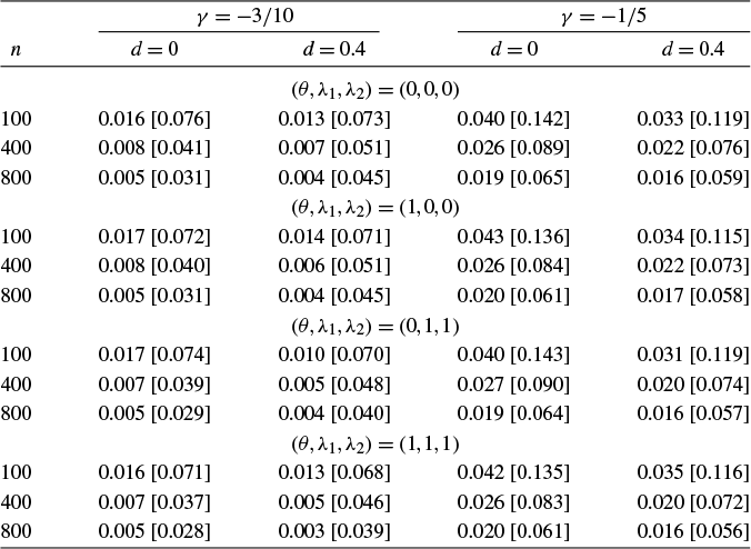
Finite sample mean bias and standard error (in square brackets) of the local level estimator
 $\hat {\beta }_n(x)$
at point
 $x=0$
for model M1 with
 $h=0.5n^{\gamma }$

The pointwise estimation accuracy of the local level estimator
 $\hat {\beta }_n(x)$
in model M1 is reported in Table 1. The two figures in each entry are the finite sample bias and standard error (shown in square brackets). A fixed bandwidth
 $h=C_hn^{\gamma }$
is used, where the constant scale coefficient
 $C_h$
and power parameter
 $\gamma $
are indicated in the table. Here, and later for model M2, a fixed bandwidth
 $h=C_hn^{\gamma }$
is used in demonstrating the performance of the local level and local linear estimators. The usual bandwidth formula
 $h=C_h\hat {\sigma }_xn^{\gamma }$
is inappropriate in the present context because the standard deviation of a nonstationary regressor or covariate diverges and this typically leads to bandwidth divergence.
The left panel with
 $\gamma =-3/10$
meets the bandwidth condition given in Theorem 4.1, whereas the right panel with
 $\gamma =-1/5$
does not. When
 $(\theta ,\lambda _1,\lambda _2)=(0,0,0)$
,
 $x_k$
and
 $y_k$
are independent and both are independent of the equation error
 $u_k$
. Other scenarios demonstrate finite sample performance when that independence is removed. The local level estimator seems to work well with diminishing bias and standard error as n increases in all the scenarios considered. The performance is not sensitive to the correlation parameters
 $(\theta ,\lambda _1,\lambda _2)$
, thereby indicative of robustness, including robustness to endogeneity in the regression, a result that mirrors earlier findings on nonparametric cointegrating regression in Reference Wang and PhillipsWP2009b. A larger bandwidth choice with higher
 $\gamma $
seems to make both bias and standard error worse, as may be expected. On the other hand, a larger memory parameter d raises signal strength and helps to reduce the bias. These results are obtained using a fixed given bandwidth. It might be expected that improved results could be achieved with variable bandwidth choices better suited to the specific generating mechanism. The present limit theory only provides general guidance and optimal bandwidth results are well known to be scarce in nonstationary nonparametric regression, although Wang and Phillips (Reference Wang and Phillips2023) provide some findings for nonlinear cointegrated regression. The difficulties of developing a general theory of optimal bandwidth choice are substantially greater here with nonstationarity in the covariate as well as the regressor.
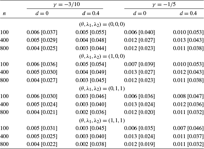
Table 2 collects parallel results for the local linear estimator
 $\hat {\beta }_L(x)$
. The local linear estimator is much more sensitive to bandwidth than the local level estimator. Poor bandwidth choice may cause the bias and/or standard error to increase and make the estimator seem inconsistent. When
 $\gamma =-1/5$
, which does not satisfy the bandwidth condition in Theorem 4.2, the bias seems to increase from
 $n=100$
to
 $400$
, and then decrease from
 $n=400$
to
 $800$
. We have tried increasing the sample size and confirmed that the bias is decreasing, but at a very slow rate. Results with
 $\gamma =-3/10$
seem satisfactory. The results again seem insensitive to the correlation parameter
 $(\theta ,\lambda _1,\lambda _2)$
, showing that the local linear estimator retains robustness to endogeneity. The bias is smaller and the standard error is larger when there is stronger memory in
 $\xi _k$
(larger d). Compared to the results in Table 1, the findings for the local linear estimator indicate that it outperforms the local level estimator in terms of both bias and standard deviation under the same bandwidth conditions.
Finite sample mean bias and standard error (in square brackets) of the local linear estimator
 $\hat {\beta }_L(x)$
at point
 $x=0$
for model M1 with
 $h=0.5n^{\gamma }$

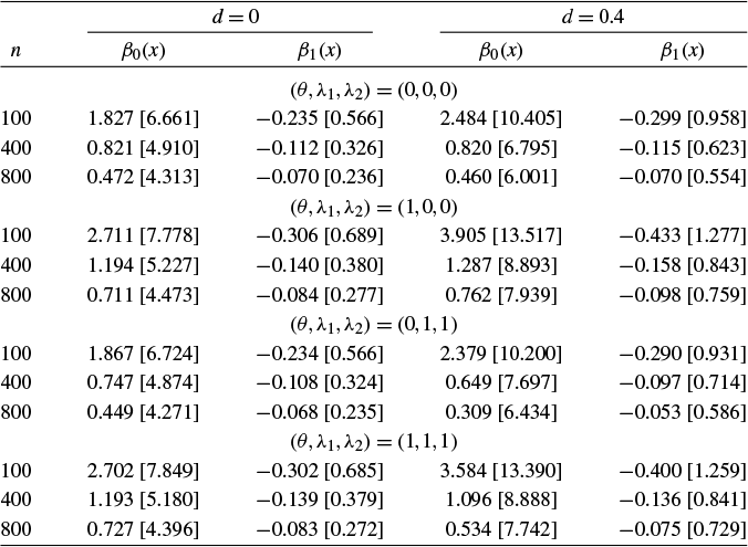
We next consider model M2. The finite sample bias and standard error of the local level estimator for the two functional coefficients are collected in Table 3. We use
 $h=1.5n^{-3/10}$
with an increased scale coefficient
 $C_h=1.5,$
which helps to avoid near singularity in the weighted signal matrix. The results show that the slope coefficient
 $\beta _1(x)$
is more accurately estimated than the intercept coefficient
 $\beta _0(x)$
, reflecting the different signal strengths in the corresponding regressors. Also noted is that estimation accuracy deteriorates as the memory parameter d increases. The explanation is simply that with stronger memory in
 $\xi _{k}=\Delta x_k$
, the covariate
 $x_k$
wanders more extensively, leading to fewer observations being available in local estimation. Estimation is again seen to be insensitive to the correlation parameters
 $(\theta ,\lambda _1,\lambda _2)$
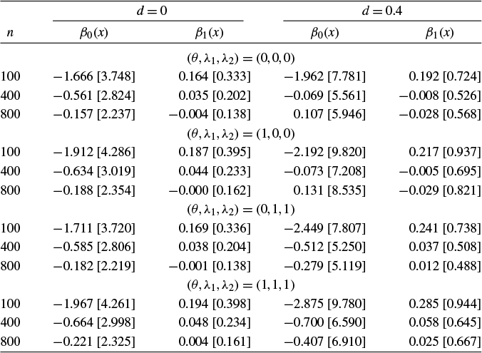
, showing that robustness to endogeneity applies in the estimation of model M2 also. Table 4 reports similar results for the local linear estimator
 $\widetilde {\widehat \beta _L}(x)$
. The estimator performance is extremely sensitive to bandwidth, especially when
 $d=0.4$
. A larger scale coefficient
 $C_h=2$
is used to avoid singularity in the weighted signal matrix. Results in the SM case with
 $d=0$
show monotonically decreasing bias and standard error. In the LM case with
 $d=0.4$
, the bias sometimes does not decay monotonically. These simulation findings suggest that estimator performance in this scenario is extremely sensitive to bandwidth. Consequently, it appears that finding an appropriate bandwidth selection rule that applies in all situations with a diverse range of nonstationarity in the variables is a challenging problem for future investigation.
Finite sample mean bias and standard error (in square brackets) of the local level estimator at point
 $x=0$
for model M2 with bandwidth
 $h=1.5n^{-3/10}$

Finite sample mean bias and standard error (in square brackets) of the local linear estimator at point
 $x=0$
for model M2 with bandwidth
 $h=2n^{-3/10}$

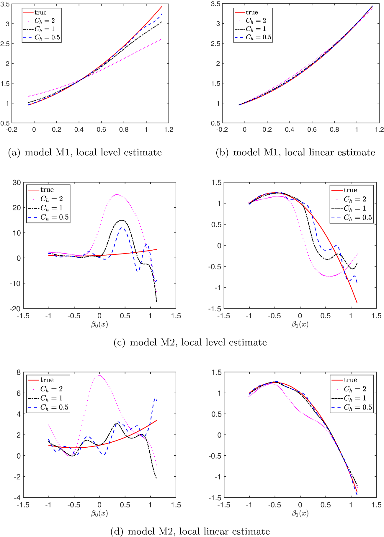
In terms of the overall estimation accuracy of the functional coefficient curves, Figure 1 provides an illustrative example based on a typical replication and use of a fixed bandwidth
 $h=C_h n^{-3/10}$
with
 $C_h\in \{0.5,1,2\}$
. Bandwidth choice clearly affects performance and local linear estimation generally outperforms local level estimation. For model M2, the slope coefficient
 $\beta _1(x)$
is estimated more precisely than the intercept coefficient
 $\beta _0(x)$
, as expected.
A representative demonstration of the curve estimates with
 $n=400$
,
 $h=C_h n^{-3/10}$
,
 $d=0,$
and
 $(\theta ,\lambda _1,\lambda _2)=(0,0,0)$
.

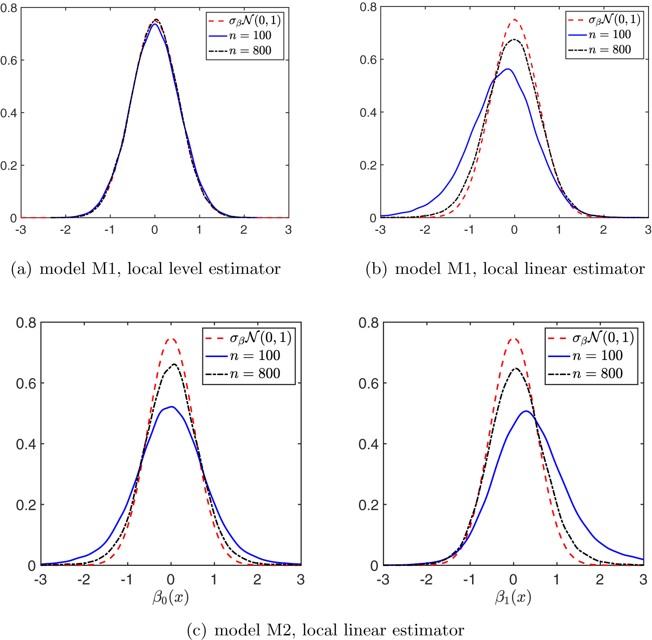
Further, to illustrate how well asymptotic results approximate the finite sample behavior of the estimators, we plot the empirical densities of the self-normalized quantities studied in Theorems 4.1–4.3. Specifically, the empirical densities of the left-hand side quantities in equations (4.4), (4.9), and (4.13) are plotted and shown against the respective limiting normal density. The unknown
 $\beta (x)$
,
 $\beta '(x)$
,
 $\beta "(x),$
and
 $\sigma ^2$
are replaced with true values. The results are displayed in Figure 2. The findings here are not sensitive to d and
 $(\theta ,\lambda _1,\lambda _2)$
but they are sensitive in estimation accuracy to bandwidth, as we have observed. As is well-known, the usual advantage of local linear estimation is to reduce bias and improve performance near the boundary. It is interesting to notice that here, while the bias terms are included to ensure the asymptotic normality as given in Theorems 4.1–4.3, the density of the local level estimator appears to be better approximated by limit behavior than that of the local linear estimator, as indicated in Figure 2(a). In sum, the finite sample densities are generally close to and appear to be converging to the asymptotic distribution, corroborating the limit theory of Theorems 4.1–4.3.


These simulation findings in the present functional coefficient model setting, where both the regressor
 $y_k$
and the smoothing covariate
 $x_k$
are nonstationary, show that nonparametric estimation can be very sensitive to bandwidth. This sensitivity is found to become severe when there are multiple regressors and local linear methods are used. Poor choice of bandwidth can worsen finite sample performance, sometimes with increasing bias and/or variance even as the sample size rises from
 $n=100$
to
 $n=400$
, and larger sample sizes are needed to obtain improvements in performance. This high sensitivity is primarily due to the random wandering nature of the covariate
 $x_k$
and its functional interaction with the nonstationary regressor
 $y_k$
by virtue of the nonparametric treatment of the functional coefficient. Standard cross validation, which is not validated in the present setting of dual-source nonstationarity, does not materially improve matters even if implemented within each replication. Use of small bandwidths typically increases the risk of the locally weighted signal matrix being close to singular, leading to a form of ill-posed inverse problem analogous to, but originating differently from that which arises in certain microeconometric instrumental variable regressions (e.g., Hall and Horowitz, Reference Hall and Horowitz2005). Problems of this type also arise in nonparametric regression whenever signal information is limited to very few observations, as when strong effects of long memory are present in the data (e.g., Wang and Phillips, Reference Wang and Phillips2024). In such circumstances, estimation can become volatile and unreliable, which in turn interferes with the performance of methods such as cross validation. It therefore appears that such problems as ill-posed inversions and the curse of dimensionality in nonparametric estimation are exacerbated in the functional coefficient dual-source nonstationary setting. Tackling these issues systematically using methods, such as regularization, is a challenging task to be addressed in future research.
5.1 Test Performance
This section examines the finite sample performance of the two test statistics proposed in Section 4.1. First, convergence in both (3.3) and (4.21) is found to be slow and the finite sample density of
 $T_{n,0}$
is more concentrated at the origin than that of the limit
 $\tau _0L_X(1,0)$
, which results in severe under-sizing. Second, the density of
 $\widetilde {T}_n/\sqrt {2\tilde {\sigma }_n^2}$
is biased to the left and has smaller variance than the standard normal, leading to bias distortion. The wild bootstrap procedure is adopted to improve the finite sample performance of these statistics. Our experiments focus on model M2 to provide more useful insight on the performance of the tests that are employed in the empirical work.
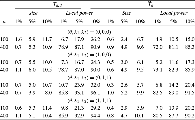
In the short memory case with
 $d=0$
, the bootstrap size and local power of the two statistics are reported in Table 5. The bandwidth is
 $h=n^{-1/3}$
, which meets the requirements in Theorems 4.4 and 4.5. We consider
 $H_0:\beta _0(x)=1+z,\beta _1(x)=1$
and
 $m(x)=x^2$
,
 $\rho _{n}=n^{-1/15}$
, which satisfy the conditions in Remark 4.7. From Table 5, it is evident that both tests have good size and local power performance. The
 $\widetilde {T}_n$
statistic is slightly undersized when
 $n=100$
but has good size when
 $n=400$
. The
 $T_{n,d}$
statistic seems somewhat more powerful than the
 $\widetilde {T}_n$
statistic. Importantly, dependence between
 $x_k$
and
 $y_k$
and endogeneity in
 $(x_k,y_k)$
have negligible effects on test performance. These finite sample properties of the tests support the use of the bootstrap procedure in empirical work such as the climate data sensitivity application in Section 6.
Finite sample size and local power of bootstrap procedure in model M2 with
 $d=0$

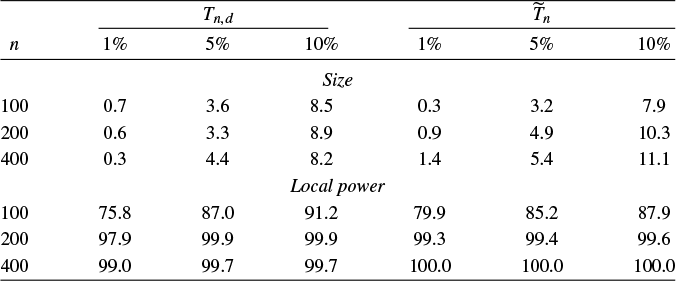
We also examined the performance of the bootstrap procedure in the LM case with
 $d=0.4$
. This implementation works under the assumption of SM innovations (with
 $d=0$
), whereas the true generating mechanism has
 $d=0.4$
. The results are collected in Table 6 with
 $(\theta ,\lambda _1,\lambda _2)=(0,0,0)$
. Results for other combinations of
 $(\theta ,\lambda _1,\lambda _2)$
are similar and are omitted. Evidently, both statistics are seen to be slightly undersized when n is small. When
 $n=400$
, the statistic
 $T_{n,d}$
still suffers from undersizing but
 $\widetilde {T}_n$
has good size performance. This outcome matches the conjecture in Wang and Phillips (Reference Wang and Phillips2016) that
 $T_{n,d}$
would become more conservative as d increases. What may be unexpected in the findings is the high power performance. Since the statistics themselves are not designed to accommodate long memory, and the limit theory of the bootstrap is not investigated here, these properties are issues left for future research.
Finite sample size and local power performance in model M2 with
 $d=0.4$
and
 $(\theta ,\lambda _1,\lambda _2)=(0,0,0)$

6 APPLICATION TO GLOBAL CLIMATE SENSITIVITY
As an application of our methods, we consider the problem of estimating Earth’s climate sensitivity to a given increase in atmospheric CO
 $_2$
concentration. As described in Storelvmo et al. (Reference Storelvmo, Heede, Leirvik, Phillips, Arndt and Wild2018), this is an issue on which there is much ongoing research, primarily with the use of large-scale global climate models. In these global climate modeling exercises, analysis relies on computer simulation data generated from immensely detailed models of Earth’s climate using an ensemble of initializations of the variables that help to assess model sensitivity. An alternative approach that instead relies on observational data is to use econometric methods to fit much simpler dynamic panel models from which parameter estimates may be obtained to assess the impact on climate of rising atmospheric CO
 $_2$
concentrations. The methodology has been developed in recent work by Magnus, Melenberg, and Muris (Reference Magnus, Melenberg and Muris2011), Storelvmo et al. (Reference Storelvmo, Leirvik, Lohmann, Phillips and Wild2016), and Phillips, Leirvik, and Storelvmo (Reference Phillips, Leirvik and Storelvmo2020). An advantage of the approach is that observationally based confidence intervals may be constructed for the key parameters that are involved in measuring climate change dynamics and the long-term impact of rising CO
 $_2$
concentrations. Recent research (Storelvmo et al., Reference Storelvmo, Yuan, Leirvik, Alterskjær, Phillips and Smith2025) indicates that the use of observational data, rather than climate model simulations from multiple ensembles, helps to narrow the confidence interval in the estimation of the Earth’s climate sensitivity.
Our application here uses three observational data sets: temperature (
 $T_{it}$
), surface level solar radiation (
 $R_{it}$
), and CO
 $_2$
equivalent greenhouse gas concentrations (CO
 $_{2,t}$
). The temperature and surface radiation data record time series at multiple surface stations and thereby conform to usual panel data with individual station and time series observations, whereas the CO
 $_2$
data varies only over the temporal dimension. Since a primary goal of empirical research with this data is to measure the recent historical impact of aggregate CO
 $_2$
on Earth’s climatic temperature, the panel model framework necessarily involves the use of time and station level series in conjunction with possible communal variables that affect climate in aggregate. Such communal variables in the present case are aggregate CO
 $_2$
levels and aggregate solar radiation levels measured at the Earth’s surface.
It is convenient in this application to use the same base dataset as in Phillips et al. (Reference Phillips, Leirvik and Storelvmo2020), which is recorded over the 42-year period from 1964 to 2005 over 1,484 land-based observation stations. Phillips et al. (Reference Phillips, Leirvik and Storelvmo2020) use aggregate data in their empirical work, basing their formulation on an aggregated version of the panel model in Storelvmo et al. (Reference Storelvmo, Leirvik, Lohmann, Phillips and Wild2016) to focus directly on Earth’s climate sensitivity to CO
 $_2$
. As explained in Phillips et al. (Reference Phillips, Leirvik and Storelvmo2020), there are technical challenges in using a panel model (particularly nonstationarity in the data, co-relationships among the time series, and weak dependence in the innovations) to achieve consistent estimation and valid asymptotic inference of this global quantity. These considerations led to an aggregate model that was developed under specific conditions concerning aggregation (Phillips et al., Reference Phillips, Leirvik and Storelvmo2020, Assumption A(i)–(v)). That model relates closely to the models given below in (6.1) and (6.2). Using these models and aggregated data in the present work enables comparisons of various nonlinear functional coefficient specifications with the linear specifications employed in Phillips et al. (Reference Phillips, Leirvik and Storelvmo2020). For example, we are able to assess whether the impact of CO
 $_{2}$
works nonlinearly through the functional coefficients or simply linearly as a common time effect regressor. For more information about the data, see Phillips et al. (Reference Phillips, Leirvik and Storelvmo2020) and Storelvmo et al. (Reference Storelvmo, Leirvik, Lohmann, Phillips and Wild2016) and the references therein.Footnote
5
Figure 3 plots the aggregated time-series data.Footnote
6
An obvious feature of these aggregate data series is their nonstationarity. Trend characteristics of varying types are evident in the global temperature, radiation, and CO
 $_2$
series, with greater year-to-year volatility in temperature and radiation than in CO
 $_2$
. These series were modeled in Phillips et al. (Reference Phillips, Leirvik and Storelvmo2020) by allowing for stochastic and deterministic linear trends as well as linear cointegrating linkages among the three aggregate series. As might be expected, much greater variation occurs in the disaggregated station-level data. Linear cointegrating regression analysis was used in Phillips et al. (Reference Phillips, Leirvik and Storelvmo2020) in studying the aggregate series and an asymptotic theory for the estimated coefficients was obtained, including asymptotics for a composite parameter that measures climate sensitivity to CO
 $_2$
.
Time-series plot of station-averaged temperature (
 $\overline {T}_t$
,
 $^{\circ }$
Celsius; blue solid), downward surface radiation (
 $\bar {R}_t$
, Watts per
 $m^2$
; red dashed), and logarithms of CO
 $_2$
(Pg: metric gigatons; black dotted with circle markers) ranging from 1964 to 2005.

In Magnus et al. (Reference Magnus, Melenberg and Muris2011) and Storelvmo et al. (Reference Storelvmo, Leirvik, Lohmann, Phillips and Wild2016), disaggregated station-level data were employed, standard linear dynamic panel within group and GMM methods were used in estimation, and no attention was paid to possible nonstationarity in the data or nonlinearity in the relationships. The present application utilizes the nonparametric regression modeling methodology developed here, allowing for the presence of functional regression coefficients that depend on an aggregate variable with nonstationary trending characteristics. The goal of the application is to assess the impact of the global influences on Earth’s temperature of CO
 $_2$
and surface (downwelling) solar radiation and to determine whether linear specifications of the type used in earlier research are justified. The implementation of this article’s methodology that follows specifically addresses nonstationarity in the aggregate data. So estimates and confidence intervals obtained in fitting the functional coefficient regression (6.1) in our empirical work below are supported by the theory of the present article.Footnote
7
We first investigate the relation among these three variables using the aggregated time-series data plotted in Figure 3. The nonstationarity in each of these variables is plainly evident in the figure and confirmed in the analysis reported in Phillips et al. (Reference Phillips, Leirvik and Storelvmo2020). Both
 $\overline {T}_t$
and
 $\bar {R}_t$
were found to be well characterized as unit-root processes and
 $\ln {CO}_2$
as a unit-root process with drift. Upon suitable normalization, these variables therefore satisfy the requirements of Assumptions A1–A3.Footnote
8
To explore the sensitivity of temperature to CO
 $_2$
, earlier work in the literature has used linear regression of temperature on CO
 $_2$
via linear modeling or linear cointegration modeling, as in Phillips et al. (Reference Phillips, Leirvik and Storelvmo2020). To allow for a possibly nonlinear coefficient impact of CO
 $_2$
on temperature, where aggregate levels of downwelling radiation may potentially affect the impact of CO
 $_2$
, we use the functional coefficient regression formulation
 $$ \begin{align} \overline{T}_t=\beta_0(\bar{R}_t)+\beta_1(\bar{R}_t)\ln(CO_{2,t})+e_t, \end{align} $$
where
 $ \overline {T}_t$
and
 $\bar {R}_t$
denote the cross-station average of
 $T_{it}$
and
 $R_{it}$
, respectively. The estimated functional coefficients from local linear regression and the corresponding asymptotic 95% confidence bands based on the limit theory in Theorem 4.3 are plotted in Figure 4. The bandwidth used is
 $h=2n^{-3/10}$
, following the guidance obtained from Table 4 in the simulations. The fitted functional coefficient estimates show that the intercept function
 $\beta _0(\bar {R}_t)$
exhibits an upward trend with radiation, suggesting that the level impact on temperature rises with solar radiation, as expected. On the other hand, the slope coefficient function
 $\beta _1(\bar {R}_t)$
exhibits a downward trend, suggesting lower correlation between temperature and CO
 $_2$
when radiation is higher. This outcome may be partly explained by the fact that downwelling solar radiation rises when atmospheric conditions are clearer with less pollutants (like sulfur dioxide), and in such cases, the greenhouse gas effects of rising CO
 $_2$
on temperature may be attenuated because of greater infrared radiation into space and aerosol/cloud interactions (Wild, Reference Wild2012).
Estimated functional coefficients of model (6.1).

To see whether the linear relation assumption between temperature and CO
 $_2$
is supported by the data, we consider the following partial linear model:
 $$ \begin{align} \overline{T}_t=\beta_0(\bar{R}_t)+\beta_1 \ln(CO_{2,t})+v_t. \end{align} $$
The estimated curve of
 $\beta _0(\bar {R}_t)$
is plotted in Figure 5 with 95% confidence bands, and the estimate of
 $\beta _1$
is 4.20 with the 95% confidence interval
 $[3.47,4.92].$
Footnote
9
The estimated curve
 $\beta _0(\bar {R}_t)$
in Figure 5 shows a clear upward trend, revealing strong positive effects from radiation to temperature. To test the constancy of
 $\beta _1(\bar {R}_t)$
in model (6.1), or equivalently, the linear relation assumption between temperature and CO
 $_2$
, we employ the generalized likelihood ratio (GLR) test of Fan, Zhang, and Zhang (Reference Fan, Zhang and Zhang2001) to test the null model of (6.2) against the alternative model of (6.1). The test gives a p-value of 0.52,Footnote
10
suggesting a failure to reject the linear relationship between temperature and CO
 $_2$
that embodies the positive impact of radiation on temperature through the radiation-dependent intercept.
Estimated functional coefficient
 $\beta _0(\bar {R}_t)$
of model (6.2).

To further investigate the nature of the impact of radiation on temperature, we consider testing the constancy of
 $\beta _0(\bar {R}_t)$
in model (6.2). The GLR test gives a p-value of 0.019, suggesting rejection of the commonly used simple linear model
 $ \overline {T}_t=\beta _0+\beta _1 \ln (CO_{2,t})+\epsilon _t.$
This result strongly demonstrates the significant role of radiation on temperature. Moreover, from the estimated curve shown in Figure 5 for the intercept function, it seems that radiation has an approximate linear impact on temperature. We therefore proceed to test whether
 $\beta _0(\bar {R}_t)$
in model (6.2) can be accepted as a linear function of
 $\bar {R}_t$
. That is, we test a linear model of the following form:
 $$ \begin{align} \overline{T}_t=\alpha_0+\alpha_1 \bar{R}_t+\beta_1 \ln(CO_{2,t})+\varepsilon_t, \end{align} $$
against the partial linear model in (6.2). Using the GLR test gives a p-value of 0.75, suggesting that the linear specification in (6.3) adequately captures the dependence of temperature on radiation and CO
 $_2$
. In addition, the two test statistics proposed in Section 4.1 were used to test the null model of (6.3) against the functional coefficient model (6.1). Both statistics returned p-values greater than 0.4, which again support the linear model specification in (6.3). The linear model in (6.3) has precisely the form of the global linear (cointegrating) relation among the variables that was used in Phillips et al. (Reference Phillips, Leirvik and Storelvmo2020).
These empirical findings show that functional coefficient regression models can be helpful in guiding and justifying parametric specifications when both nonstationary covariates and nonstationary regressors are present. The nonparametric regression results and functional specification tests obtained provide empirical support for the aggregate linear models that have recently been used in climate econometric research to study the impact on temperature of
 $CO_{2}$
greenhouse gases and downwelling solar radiation.
7 CONCLUSION
While this article adds to existing limit theory and widens the field of potential applications of nonlinear regressions with nonstationary time series, there is scope for further extension. Some additions that would extend the present theory involve relaxing the mds condition on the equation error
 $u_t$
, developing bias reduction methods, and coping with further induced endogeneity. In the context of TVP cointegration, Phillips et al. (Reference Phillips, Li and Gao2017) developed a version of fully modified regression that worked successfully in that context. General forms of the regression model (4.1) with nonlinear functional coefficient vector
 $\beta (x_k)$
and stationary errors have considerably more complex elements and it seems that new methods may be needed to achieve these extensions. This work is left for future research.
Simulations are generally supportive of the functional coefficient limit theory in the presence of both a nonstationary regressor and smoothing covariate. But our findings reveal that finite sample performance is affected by reduced local signal strength and increased sensitivity to bandwidth choice. These issues are exacerbated in multiple regressor cases and in the use of local linear estimation. They arise from the random wandering nature of the covariate
 $x_k$
and its functional interaction with the nonstationary regressor
 $y_k$
. The combined impact of this dual-source nonstationarity in regression is to reduce kernel-weighted signal strength in the relevant estimation locality by virtue of the nonparametric treatment of the functional coefficient. Small bandwidths typically reduce the number of relevant observations and raise the risk of singularity in the locally weighted signal matrix. Increasing the bandwidth helps to resolve the ill-posed inversion but also raises bias in the regression. Thus, while the originating source differs from existing ill-posed inverse problems in econometrics, some of the effects turn out to be similar. Addressing this issue and the curse of dimensionality in nonstationary nonparametric regression is a further challenge for future research.
8 Proofs
Proof of Proposition 2.1
It is routine to see that
 $var(y_n)/n\to \,\Gamma $
, where
 $\Gamma =\alpha ^{\mathrm T} \Psi \,\Omega \Psi ^{\mathrm T}\alpha .$
As for (2.2), by A2′
(ii), we have
 $$ \begin{align} \left( \frac{1}{\sqrt{n}} \sum_{i=1}^{\lfloor nt\rfloor }\epsilon _{-i},\ \frac{1 }{\sqrt{n}}\sum_{i=1}^{\lfloor nt\rfloor }\epsilon _{i},\ \frac 1{\sqrt n} \sum_{j=1}^{[nt]}\eta_j\right) \Rightarrow& Z_t:=(B_{-t}, B_t, \Lambda_t), \end{align} $$
where
 $Z=\{Z_t\}_{t\ge 0}$
is a
 $(2+d)$
-dimensional Gaussian process with mean zero, independent increments, and covariance matrix
 $$ \begin{align*}\Omega_t=t\, \left(\begin{matrix}1& 0 &0\\ 0&1& \gamma^{\mathrm T}\\ 0&\gamma&\Omega\end{matrix}\right),\quad \text{where }\gamma=(\gamma_1,\ldots,\gamma_d)^{\mathrm T} \text{with } \gamma_k=E(\epsilon_0\eta_{0k}).\end{align*} $$
Therefore, it follows from A2′ (i) and Phillips and Solo (Reference Phillips and Solo1992) that
 $$ \begin{align*} \frac {y_{k}}{\sqrt n} =& \alpha^{\mathrm T} \Psi\, \frac 1{\sqrt n}\, \sum_{j=1}^{k}\eta_j +o_P(1) \end{align*} $$
and, on
 $D_{{\mathbb R}^3}[0,1]$
,
 $$ \begin{align} \left( \, \frac{1}{\sqrt{n}} \sum_{i=1}^{\lfloor nt\rfloor }\epsilon _{-i},\ \frac{1 }{\sqrt{n}}\sum_{i=1}^{\lfloor nt\rfloor }\epsilon _{i},\ \frac {y_{[nt]}}{\sqrt n}\,\right) \Rightarrow& (B_{-t},\ B_t, \ \alpha^{\mathrm T} \Psi\, \Lambda_t), \end{align} $$
implying (2.2).
Proof of Theorem 3.1
We only prove (3.1) since the joint convergence (3.2) is immediate after some routine notation changes in view of (2.3). We first assume that
 $g(x)$
is bounded and continuous on
 ${\mathbb R}$
. This restriction will be removed later. Write
 $$ \begin{align*} L_{1n, \epsilon} &= \frac {1}n\,\sum _{k=1}^n g(Y_{nk})\, \phi_{\epsilon} (X_{nk}) \int_{-\infty}^\infty f(x)dx, \\ L_{2n,\epsilon}&= \frac {c_n}{n}\,\sum_{k=1}^ng(Y_{nk}) \int_{-\infty}^{\infty} f\big[ c_n\,( X_{nk}+z\epsilon)\big] \phi(z)dz, \end{align*} $$
where
 $\phi _{\epsilon }(x)=\frac 1{\epsilon \sqrt { 2\pi }}\exp \big \{-\frac {x^2}{2\epsilon ^2}\big \}$
and
 $\phi (x)=\phi _1(x)$
. Recalling (2.3), it follows from the continuous mapping theorem, the occupation time formula, and (2.6) with
 $a(x)=\phi (x)$
that
 $$ \begin{align*} L_{1n, \epsilon} \Rightarrow &\int_0^1g(Y_t)\,\phi_\epsilon(X_t)dt\, \int_{-\infty}^\infty f(x)dx \quad (\text{as }n\to\infty) \\ =&\int_{-\infty}^{\infty} \int_0^1 g(Y_t)\, \phi_\epsilon(x)\, L_X (dt, x)\, dx\, \int_{-\infty}^\infty f(x)dx \\ & \quad \text{(by the occupation time formula)}\\ =&\int_{-\infty}^{\infty}\phi(x)\, \int_0^1 g(Y_t)\,L_X (dt, \epsilon x) dx\, \int_{-\infty}^\infty f(x)dx \\ \to_{a.s.}& \int_0^1 g(Y_t)L_X (dt, 0)\, \int_{-\infty}^\infty \phi(x)dx\, \int_{-\infty}^\infty f(x)dx= \mathbb{S}, \quad \text{as }\epsilon\to 0. \end{align*} $$
Result (3.1) will follow if we prove: for any
 $ \epsilon>0$
,
 $$ \begin{align} L_{1n,\epsilon}-L_{2n,\epsilon}=o_P(1), \end{align} $$
and, as
 $n\to \infty $
followed by
 $\epsilon \to 0$
,
 $$ \begin{align} S_n-L_{2n,\epsilon} =o_P(1). \end{align} $$
We start with some basic preliminaries before proving (8.3) and (8.4). Recall A1 and
 $\lim \sup _{t\to \infty }t^{\delta }|\mathbb {E}e^{it\epsilon _0}|<\infty $
for some
 $\delta>0$
. It follows from Theorem 2.18 of Wang (Reference Wang2015) that, for all
 $k\ge 1$
,
 $x_k/d_k$
has a density
 $p_k(x)$
which is uniformly bounded by a constant C and, conditional on
 ${\cal F}_{\epsilon j}:=\sigma (\epsilon _j, \epsilon _{j-1},\ldots )$
,
 $(x_k-x_j)/d_{k-j}$
has a density
 $p_{kj}(x)$
satisfying
 $$ \begin{align} \sup_x|p_{kj}(x+u)-p_{kj}(x)|\le C\min\{|u|, 1\}, \end{align} $$
for all
 $j\ge 1$
and
 $k-j\ge n_0\ge 1$
, where the fixed constant
 $n_0$
is chosen so that
 $x_k-x_j\not =0$
. Since the finite items have no impact on the asymptotics, without loss of generality, we assume
 $n_0=1$
in the following proof. Using these facts, for any integrable function
 $l(x)$
and constant sequence
 $a_n>0$
, we have
 $$ \begin{align} \mathbb{E} | l(a_n X_{nk}) | =& \int_{-\infty}^\infty | l(a_n d_k d_n^{-1} x) |\, p_k(x) dx \ \le\ C\, a_n^{-1} (d_n/ d_k)\, \int_{-\infty}^\infty|l(x)| dx, \end{align} $$
for all
 $k\ge 1$
, and
 $$ \begin{align} &\quad\big|\mathbb{E}\big(\big\{ l(a_n X_{nk}) -l[a_n (X_{nk}+z\epsilon)]\big\} \,\mid {\cal F}_{\epsilon j}\big)\big| \nonumber\\ &= \big| \int_{-\infty}^\infty \Big\{l(a_n X_{nj}+\frac {a_nd_{k-j}}{d_n}y )- l\big[a_n (X_{nj}+z\epsilon)+\frac {a_nd_{k-j}}{d_n}y \big]\Big\} p_{kj}(y) dy\big| \nonumber\\ &= a_n^{-1} \, (d_n/ d_{k-j})\,\big| \int_{-\infty}^\infty \Big\{l(a_n X_{nj}+y )- l\big[a_n (X_{nj}+z\epsilon)+y \big]\Big\} p_{kj}\big( \frac {yd_n}{a_nd_{k-j}}\big) dy\big| \nonumber\\ &\le a_n^{-1} \, (d_n/ d_{k-j})\,\int_{-\infty}^\infty |l(y)| \, \Big|p_{kj}\Big(\frac {y-a_n X_{nj}}{a_nd_{k-j}/d_n}\Big)-p_{kj}\Big(\frac {y-a_n (X_{nj}+z\epsilon)}{a_nd_{k-j}/d_n}\Big)\Big| dy\nonumber\\ &\le C a_n^{-1} \, (d_n/ d_{k-j})\,\min\{1, d_n|z|\epsilon/d_{k-j}\}, \end{align} $$
for all
 $j\ge 1$
and
 $k-j\ge 1$
. Furthermore, by recalling that
 $a(k)$
is slowly varying at infinity, it follows from (2.1) that, for all
 $1\le l+1\le j\le n$
,
 $$ \begin{align} \sum_{k=l+1}^{j} d_k^{-1} \le C (j-l)\,d_j^{-1}, \qquad \sum_{k=1}^{j} d_k^{-2} \ \le \ C\, \left \{\begin{array}{@{}ll@{}} 1, & \text{under }\textbf{LM}, \\ \log j, & \text{under }\textbf{SM}, \end{array} \right. \end{align} $$
and, for all
 $l\le j$
and j sufficiently large,
 $$ \begin{align} C_1\, (l/j)^{1-\delta}\le d_l/d_j\le C_2\,(l/j)^{1/2}, \end{align} $$
for some
 $\mu -1/2>\delta >0$
, where
 $C_1>0$
and
 $C_2>0$
are two absolute constants.
Return to the proofs of (8.3) and (8.4). Equation (8.3) is simple. In fact, by the boundedness of
 $g(x)$
and the fact that
 $$ \begin{align*} L_{2n,\epsilon}= &\frac {1}{n}\,\sum_{k=1}^ng(Y_{nk}) \int_{-\infty}^{\infty} f(y) \phi_\epsilon(y/c_n-X_{nk})dy, \end{align*} $$
it follows from (8.6) with
 $a_n=1$
and (8.8) with
 $l=0$
and
 $j=n$
that, for any
 $\epsilon>0$
,
 $$ \begin{align*} &\mathbb{E}\,|L_{1n,\epsilon}-L_{2n,\epsilon}| \le \frac {C}{n}\,\sum_{k=1}^n \int_{-\infty}^{\infty}| f(y)|\, \mathbb{E}\, \big|\phi_\epsilon(y/c_n-X_{nk})-\phi_\epsilon(X_{nk})\big|\, dy \\ &\quad\le \frac{Cd_n}{n}\,\sum_{k=1}^nd_k^{-1} \int_{-\infty}^{\infty} |f(y)|\, \int_{-\infty}^{\infty} |\phi_\epsilon(y/c_n-x)-\phi_\epsilon(x)|dx\, dy \\ &\quad \le C\, \Big[ \int_{(|y|\ge \sqrt {c_n})} |f(y)| dy + \int_{|y|<\sqrt {c_n}} |f(y)|\, \int_{-\infty}^{\infty} |\phi_\epsilon(y/c_n-x)-\phi_\epsilon(x)|dx\, dy\Big] \\ & \quad\le C\, \Big\{\int_{|y|\ge \sqrt {c_n}}|f(y)|dy+\big[(\epsilon\sqrt {c_n})^{-1}+ (\epsilon^2 c_n)^{-1}\big]\int_{-\infty}^\infty |f(y)| dy\Big\}\\ &\quad \to 0,\quad \text{as }n\to\infty, \end{align*} $$
due to
 $c_n\to \infty $
and
 $\int _{-\infty }^\infty |f(y)| dy<\infty $
, where we have used the fact: for any
 $\delta>0 $
,
 $$ \begin{align*} & \int_{-\infty}^{\infty} |\phi_\epsilon(\delta-x)-\phi_\epsilon(x)|dx\\ &\quad \le \frac 1{\sqrt {2\pi}}\,\int_{-\infty}^{\infty} |e^{-(\delta-\epsilon x)^2/2\epsilon^2}-e^{-x^2/2}|dx \, \le\, C \big[\delta/\epsilon +(\delta/\epsilon)^2\big]. \end{align*} $$
We next consider (8.4). First note that, by the tightness of
 $\{Y_{n,[nt]}\}_{ 0\le t\le 1}$
and continuity of
 $g(x)$
,
 $$ \begin{align} \max_{1\le j\le n/m} \hspace{1mm} \max_{(j-1)m+1\le k\le jm} |g(Y_{nk})-g(Y_{n,(j-1)m+1})|=o_P(1), \end{align} $$
as
 $n\to \infty $
followed by
 $\epsilon \to 0$
, where
 $m=\lfloor n/K_{\epsilon } \rfloor $
and
 $K_\epsilon \to \infty $
as
 $\epsilon \to 0$
. We may take
 $K_\epsilon \to \infty $
sufficiently slow so that
 $\epsilon ^\eta K_\epsilon \to 0$
for any
 $\eta>0$
. Let
 $T_n=\lfloor n/m \rfloor $
. We may write
 $$ \begin{align} S_n =\ &\frac {c_n}n\,\sum_{j=2}^{T_n} \sum_{k=(j-1)m+1}^{jm} \, g(Y_{nk})\, f( c_nX_{nk} )+S_{2n, \epsilon}\nonumber\\ =\ &\frac {c_n}n\,\sum_{j=2}^{T_n} \, g(Y_{n,(j-1)m+1})\, \sum_{k=(j-1)m+1}^{jm}\, f( c_nX_{nk} ) \nonumber\\ &+\, \frac {c_n}n\,\sum_{j=2}^{T_n} \sum_{k=(j-1)m+1}^{jm} \, \big[g(Y_{nk})-g(Y_{n,(j-1)m+1})\big]\, f( c_nX_{nk} ) +S_{2n, \epsilon} \nonumber\\ :=\ & \frac {c_n}n\,\sum_{j=2}^{T_n} \, g(Y_{n,(j-1)m+1})\, \sum_{k=(j-1)m+1}^{jm}\, f( c_nX_{nk} ) +S_{1n, \epsilon}+S_{2n, \epsilon}, \end{align} $$
where
 $$ \begin{align*} |S_{2n, \epsilon}| \le& \frac {Cc_n}n \, \Big(\sum_{k=1}^{m}+\sum_{k=T_n m+1}^{n} \Big) \, | f( c_nX_{nk})|. \end{align*} $$
It follows from (8.6) with
 $a_n=c_n$
and (8.8) and (8.9) that
 $$ \begin{align*} \mathbb{E} |S_{2n, \epsilon}| &\le C\, n^{-1} d_n\, \Big(\sum_{k=1}^m d_k^{-1}+\sum_{k=n-m}^n d_k^{-1} \Big) \\ & \le C_1m/ n(1+d_n/d_m)\le C_1(m/n)^{1/2}\le C_1\,K_{\epsilon}^{-1/2}, \end{align*} $$
i.e.,
 $S_{2n, \epsilon }\to _P0$
as
 $n\to \infty $
followed by
 $\epsilon \to 0$
. Similarly, we have
 $ \frac {c_n}n\sum _{k=1}^n \big |f(c_n X_{nk})\big | =O_P(1), $
from which it follows from (8.10) that
 $$ \begin{align*} |S_{1n, \epsilon}| \le\max_{1\le j\le n/m} \hspace{1.0mm} \max_{(j-1)m+1\le k\le jm} |Y_{nk}-Y_{n,(j-1)m+1}|\, \frac {c_n}n\sum_{k=1}^n\big| f(c_nX_{nk})\big| \to_P& 0, \end{align*} $$
Taking these estimates into (8.11), we obtain
 $$ \begin{align} S_n &=\frac {c_n}n\,\sum_{j=2}^{T_n} \, g(Y_{n,(j-1)m+1})\, \sum_{k=(j-1)m+1}^{jm}\, f( c_nX_{nk} )+ S_{n, \epsilon}, \end{align} $$
where
 $S_{n, \epsilon }=o_P(1)$
as
 $n\to \infty $
followed by
 $\epsilon \to 0$
. Similarly, we have
 $$ \begin{align} L_{2n,\epsilon} &= \frac {c_n}n\,\sum_{j=2}^{T_n} \, g(Y_{n,(j-1)m+1})\, \sum_{k=(j-1)m+1}^{jm}\, \int_{-\infty}^{\infty} f\big[ c_n\,( X_{nk}+z\epsilon)\big] \phi(z)dz +L_{n,\epsilon}, \end{align} $$
where
 $L_{n, \epsilon }=o_P(1)$
as
 $n\to \infty $
followed by
 $\epsilon \to 0$
.
In terms of (8.12) and (8.13), the boundedness of
 $g(x)$
and
 $\int _{-\infty }^\infty \phi (z) dz=1$
, result (8.4) will follow if we prove:
 $$ \begin{align} \frac {c_n}n\,\sum_{j=2}^{T_n} \,|I_{jm}(\epsilon)| \to 0, \end{align} $$
as
 $n\to \infty $
followed by
 $\epsilon \to 0$
, where
 $$ \begin{align*} I_{jm}(\epsilon) =&\int_{-\infty}^{\infty}\sum_{k=(j-1)m+1}^{jm}\, \big\{ f(c_nX_{nk})- f\big[ c_n\,(X_{nk}+z\epsilon)\big]\big\} \phi(z)dz. \end{align*} $$
To this end, write
 $Z_{nk}(z, \epsilon )= f(c_n X_{nk})-f[c_n (X_{nk}+z\epsilon )]$
and
 $\Lambda _{n, j}(z, \epsilon ) =\sum _{k=(j-1)m+1}^{jm}\, Z_{nk}(z, \epsilon ).$
Note that
 $$ \begin{align} \frac {c_n}n\,\sum_{j=2}^{T_n} \mathbb{E} \,|I_{jm}(\epsilon)| \le& \sum_{j=2}^{T_n}\int_{-\infty}^\infty \frac {c_n}n\,\mathbb{E}\,\big| \Lambda_{n, j}(z, \epsilon)\big|\, \phi(z)\, dz. \end{align} $$
The proof of (8.14) involves the calculations of
 $\mathbb {E}\,\big | \Lambda _{n, j}(z, \epsilon )\big |$
in cases that
 $|z|\ge \log \epsilon ^{-1}$
or
 $|z|\le \log \epsilon ^{-1}$
so that
 $\mathbb {E} \,|I_{jm}(\epsilon )|$
has a required order as
 $n\to \infty $
followed by
 $\epsilon \to 0$
. Such a calculation is similar to (2.69) of Wang (Reference Wang2015) but with different details under the recent formation of
 $m=\lfloor n/K_{\epsilon } \rfloor $
. In fact, it follows from (8.6) with
 $a_n=c_n$
and (8.8) and (8.9) that, uniformly for all
 $z\in R$
and
 $2\le j\le T_n$
,
 $$ \begin{align} & \sum_{k=(j-1)m+1}^{jm}\big[\mathbb{E}\,|Z_{nk}(z, \epsilon)|+\mathbb{E}\,Z_{nk}^2(z, \epsilon)\big] \le C c_n^{-1}\,d_n\sum_{k=(j-1)m+1}^{jm} d_k^{-1} \nonumber\\ &\quad \le C\, c_n^{-1} m\,d_n/d_{jm}\le C\, c_n^{-1} m\,K_\epsilon^{1-\delta}. \end{align} $$
Similarly, it follows from (8.6) with
 $a_n=c_n$
and (8.7)–(8.9) that, for
 $ (j-1)m\le i\le jm $
and for any
 $|z|\le \log ^{-1} \epsilon $
(letting
 $\sum _{k=i}^l=0$
if
 $i>l$
),
 $$ \begin{align} & \sum_{k=i+1}^{jm}\,\big|\,E\big\{Z_{nk}(z, \epsilon)\, Z_{ni}(z, \epsilon)\big\}\,\big| \nonumber\\ &\quad \le \mathbb{E}\,\Big\{|Z_{ni}(z, \epsilon)|\sum_{k=i+1}^{jm} \big|\mathbb{E}\,(Z_{nk}(z, \epsilon)\mid \mathcal{F}_{i})\big|\Big\}\nonumber\\ &\quad\le C\,c_n^{-2}\, (d_n/d_i)\,\Big[\sum_{k=i+1}^{i+\epsilon m}d_{n}/d_{k-i}+ \epsilon\, \log^{-1}\epsilon\,\sum_{k=i+\epsilon m}^{ jm}(d_n/d_{k-i})^2\Big] \nonumber\\ &\quad\le C\,c_n^{-2}\, (d_n/d_i)\, \big[ \epsilon\, m \, d_n/d_{\epsilon m}+ \epsilon\, m\,\log^{-1}\epsilon\, (d_n/d_{m})\, (d_n/d_{\epsilon m})\big] \nonumber\\ &\quad\le C\,c_n^{-2}\, (d_n/d_i)\, m\, \epsilon^\delta \log^{-1}\epsilon\,K_\epsilon^{2(1-\delta)}, \end{align} $$
where we have used the facts: by (8.9),
 $d_n/d_m\le C\,(n/m)^{1-\delta }\le C\, K_\epsilon ^{1-\delta }$
and
 $$ \begin{align*} d_n/d_{\epsilon m}\le C\,\epsilon^{\delta-1}(n/m)^{1-\delta}\le C\,\epsilon^{\delta-1}\, K_\epsilon^{1-\delta}. \end{align*} $$
In terms of (8.16), uniformly for all
 $z\in R$
and
 $2\le j\le T_n$
, we have
 $$ \begin{align*} \mathbb{E}\,\big| \Lambda_{n, j}(z, \epsilon)\big| &\le \sum_{k=(j-1)m+1}^{jm}\,\mathbb{E}\,|Z_{nk}(z, \epsilon)| \, \le \, C\, c_n^{-1} m\,K_\epsilon^{1-\delta}. \end{align*} $$
It follows from (8.16) and (8.17) that, for any
 $|z|\le \log ^{-1} \epsilon $
and
 $2\le j\le T_n$
,
 $$ \begin{align*} \big(\mathbb{E}\,\big|\Lambda_{n, j}(z, \epsilon)\big| \big)^2 & \le \mathbb{E}\,\big|\Lambda_{n, j}(z, \epsilon)\big|^2=\, \mathbb{E}\,\Big[ \sum_{k=(j-1)m+1}^{jm} Z_{nk}(z, \epsilon)\Big]^2 \\ & \le \,\sum_{k=(j-1)m+1}^{jm}\, \mathbb{E}\,Z_{nk}^2(z, \epsilon)+ \,2\sum_{i=(j-1)m+1}^{jm} \sum_{k=i+1}^{jm}\,\big|\,\mathbb{E}\,\big\{ Z_{nk}(z, \epsilon)\, Z_{ni}(z, \epsilon)\big\}\,\big| \\ & \le C\, c_n^{-1} m\,K_\epsilon^{1-\delta}+ C\,m\, c_n^{-2}\, \epsilon^\delta \log^{-1}\epsilon\,K_\epsilon^{2(1-\delta)}\sum_{k=(j-1)m+1}^{jm}d_n/d_i\,\\ & \le C\, c_n^{-1} m\,K_\epsilon^{1-\delta}+ C\,m^2\, c_n^{-2}\, \epsilon^\delta \log^{-1}\epsilon\,K_\epsilon^{3(1-\delta)}\,. \end{align*} $$
Taking these estimates into (8.15) and recalling that
 $K_{\epsilon }\to \infty $
is so slow so that
 $\epsilon ^\eta K_\epsilon \to 0$
for any
 $\eta>0$
, we have
 $$ \begin{align*} \frac {c_n}n\,\sum_{j=1}^{T_n} \mathbb{E}\,|I_{jm}(\epsilon)| &\le \sum_{j=2}^{T_n}\int_{-\infty}^\infty \frac {c_n}n\,\mathbb{E}\,\big| \Lambda_{n, j}(z, \epsilon)\big|\, \phi(z)\, dz \\ &\le \frac {c_n}n\, \sum_{j=2}^{T_n}\int_{|z|\ge \log^{-1} \epsilon}\mathbb{E}\,\big| \Lambda_{n, j}(z, \epsilon)\big|\, \phi(z)\, dz \\ &\qquad \qquad + \ \frac {c_n}n\, \sum_{j=2}^{T_n}\int_{|z|< \log^{-1} \epsilon} \,\big(\mathbb{E}\,\big| \Lambda_{n, j}(z, \epsilon)\big|^2\big)^{1/2}\, \phi(z)\, dz\\ & \le C\, K_\epsilon^{1-\delta} \int_{|z|\ge \log^{-1}\epsilon}\phi(z)\, dz +\epsilon^{\delta/2} \log^{-1/2}\epsilon\,K_\epsilon^{3(1-\delta)/2} \to 0, \end{align*} $$
as
 $n\to \infty $
followed by
 $\epsilon \to 0$
. This proves (8.14) and completes the proof of (3.1) under the additional assumption that
 $g(x)$
is bounded on
 ${\mathbb R}$
.
Finally, we remove the additional restriction on the boundedness of
 $g(x)$
. For each
 $N>0, g_N(x)=g(x)\xi _N(x)$
with
 $$ \begin{align*} \xi_N(x)=\left\{ \begin{array}{@{}ll@{}} 1 & |x|\le N\\ 2-|x|/N & N<|x|<2N\\ 0 & |x|\ge 2N. \end{array} \right. \end{align*} $$
Let
 $S_{n, N} = \frac {c_n}n\sum _{k=1}^n g_N(Y_{nk}) f( c_nX_{nk})$
. Since
 $g_N(x)$
is bounded and continuous, the first part of the proof yields that, for each
 $N>0$
,
 $$ \begin{align*} S_{n, N} \to_D \mathbb{S}^N:=\int_0^1 g_N(Y_s) L_X(d s, 0)\, \int_{-\infty}^\infty f(t)dt. \end{align*} $$
This implies (3.1) without assuming the boundedness of
 $g(x)$
since
 $$ \begin{align*} & \mathbb{P}\,\big(S_n\not=S_{n, N}\big) +\mathbb{P}\,\big(\mathbb{S}\not=\mathbb{S}^N\big) \\&\quad \le \mathbb{P}\,\big(\max _{1\le k\le n}|Y_{nk}|\ge N\big)+ \mathbb{P}\,\big( \sup\limits_{0\le t\le 1} |Y_{t}|\ge N\big)\to 0, \end{align*} $$
as
 $n\to \infty $
followed by
 $N\to \infty $
, due to the facts that
 $Y_{n,[nt]}\Rightarrow Y_t$
on
 $D_{\mathbb {R}}[0,1]$
and that the limit Gaussian process
 $Y_t$
is path continuous. The proof of Theorem 3.1 is now complete.
Proof of Corollary 3.1
As in Theorem 3.1, without loss of generality, we assume that
 $g(x)$
is bounded and continuous. Recall
 $\tilde f_{1}(x)=\mathbb {E} f_1(x, \lambda _m,\ldots ,\lambda _0)dx$
and write
 $$ \begin{align*} R_{n}&= \frac{c_{n}}{n}\, \sum_{k=1}^{n}g(Y_{nk}) \big[f_1\big(c_n\,X_{nk},\lambda_k, \ldots, \lambda _{k-m}) -\tilde f_1(c_n\,X_{nk})\big]. \end{align*} $$
Since
 $\tilde f_1(x)$
is bounded and integrable, by Theorem 3.1, (3.5) will follow if we prove:
 $$ \begin{align} R_{n} &=o_P(1). \end{align} $$
To this end, we first note that (8.6) can be extended to include certain stationary variables, i.e., the following result still holds:
 $$ \begin{align*} \mathbb{E} | l(a_n X_{nk}, \lambda_k, \ldots, \lambda_{k-m}) | \, \le C\, a_n^{-1} (d_n/ d_k)\, \int_{-\infty}^\infty \mathbb{E} |l(x, \lambda_m, \lambda_{m-1},\ldots, \lambda_0)| dx, \end{align*} $$
for any
 $k\ge m+m_0$
and some fixed
 $m_0>0$
. See Lemma 7.1 of Wang et al. (Reference Wang, Phillips and Kasparis2021), for instance. Now, the same argument as in the proof of (8.11) yields that
 $$ \begin{align} R_{n} =\ & \frac {c_n}n\,\sum_{j=2}^{T_n} \, g(Y_{n,(j-1)m+1})\, \sum_{k=(j-1)m+1}^{jm}\, \big[f_1\big(c_n\,X_{nk},\lambda_k, \ldots, \lambda _{k-m}) -\tilde f_1(c_n\,X_{nk})\big] \nonumber\\ &+R_{n, K}, \nonumber\\ :=\ &\frac {m}{n}\,\sum_{j=2}^{T_n} \, g(Y_{n,(j-1)m+1})\, \frac {c_n}m L_{mj}+R_{n, K,} \end{align} $$
where
 $m=\lfloor n/K \rfloor $
,
 $T_n=\lfloor n/m \rfloor ,$
and
 $R_{n, K}\to _P 0$
, as
 $(n, K)_{\textrm {seq}} \to \infty $
. As in the proof of (7.37) with
 $i=2$
in Wang et al. (Reference Wang, Phillips and Kasparis2021), we have
 $$ \begin{align*} \frac {c_n}m \,\mathbb{E} |L_{mj}|\le \big( \mathbb{E} \big |\frac {c_n}m \,L_{mj}\big|^2 \big)^{1/2}\to 0, \end{align*} $$
uniformly for
 $2\le j\le T_n\le K+1$
as
 $(n, K)_{\textrm {seq}} \to \infty $
. It follows from the boundedness of
 $g(x)$
that
 $$ \begin{align*} \frac {m}{n}\,\sum_{j=2}^{T_n} \, |g(Y_{n,(j-1)m+1})|\, \mathbb{E}\, \big| \frac {c_n}m L_{mj} \big| \le C\, \max_{2\le j\le K+1} \frac {c_n}m \,\mathbb{E} \, |L_{mj}| \to 0, \end{align*} $$
i.e.,
 $\frac {m}{n}\,\sum _{j=2}^{T_n} \, g(Y_{n,(j-1)m+1})\, \frac {c_n}m L_{mj}\to _P 0$
, as
 $(n, K)_{\textrm {seq}} \to \infty $
. Taking this estimate into (8.19), we obtain (8.18), which completes the proof of Corollary 3.1.
Proof of Theorem 3.2
We only prove (3.7) and assume
 $c_n'=0$
. The extension to general
 $c_n'$
is standard (e.g., Reference Wang and PhillipsWP2009a) and (3.6) is similar except simpler. Note that
 $M_{1n}=\sum _{k=1}^n m_{nk} u_k$
, where
 $m_{nk}=\big (\frac {c_{n}}{n}\big )^{1/2}g(Y_{nk}) f_1(c_n\,X_{nk}, \lambda _k, \ldots , \lambda _{k-m})$
depending only on
 $\lambda _k, \lambda _{k-1},\ldots $
. We may establish (3.7) by using the extended martingale limit theorem given in Wang (Reference Wang2014). To this end, let
 $\tilde g_\eta (x)=|g(x)|^{2+\eta }$
and
 $\tilde f_\eta (x, y)=|f_1(x, y)|^{2+\eta }$
. Due to A5(i), there exists a bounded and integrable function
 $\tilde T(x)$
so that, for any
 $-1\le \eta \le 1/\beta ,$
 $$ \begin{align*} |\tilde f_\eta(x,y)\big| \le& \tilde T(x)(1+|y|^{(2+\eta)\beta}), \end{align*} $$
i.e., A5(i) still holds if we replace
 $f_1$
by
 $\tilde f_\eta $
and
 $\beta $
by
 $(2+\eta )\beta $
. Since
 $\tilde g_\eta (x)$
is still continuous, it follows from Corollary 3.1 (with g and
 $f_1$
replaced by
 $\tilde g_\eta $
and
 $\tilde f_\eta $
, respectively) that
 $$ \begin{align} & \Big(\frac {1}{\sqrt n}\sum_{k=1}^{[nt]}\epsilon_k, \ \frac {1}{\sqrt n}\sum_{k=1}^{[nt]}\epsilon_{-k},\ X_{n, [nt]},\ Y_{n, [nt]}, \frac{c_{n}}{n}\sum_{k=1}^n \tilde g_\eta(Y_{nk}) \tilde f_\eta\big(c_n\,X_{nk}, \lambda_k, \ldots, \lambda _{k-m}\big)\Big)\nonumber\\ &\quad\Rightarrow \ \Big(B_t,\ B_{-t},\ X_t, \ Y_t, \int_0^1 \tilde g_\eta (Y_s) d L _{X}(s, 0)\, \mathbb{E} \tilde f_\eta(x, \lambda_m, \lambda_{m-1}, \ldots, \lambda _{0})dx\Big), \end{align} $$
for any
 $-1\le \eta \le 1/\beta .$
Consequently, it is readily seen that
 $$ \begin{align*} \max_{1\le k\le 1} |m_{nk}| \le \Big[ \big(\frac{c_{n}}{n}\big)^{1+1/(2\beta)}\sum_{k=1}^n \tilde g_{1/\beta}(Y_{nk}) \tilde f_{1/\beta}\big(c_n\,X_{nk}, \lambda_k, \ldots, \lambda _{k-m}\big)\Big]^{2\beta/(1+2\beta)}\!\!=o_P(1) \end{align*} $$
and
 $$ \begin{align*} \frac 1{\sqrt n}\sum_{k=1}^n|m_{nk}| = c_n^{-1/2}\, \frac {c_n}n\, \sum_{k=1}^n \tilde g_{-1}(Y_{nk}) \tilde f_{-1}\big(c_n\,X_{nk}, \lambda_k, \ldots, \lambda _{k-m}\big) =o_P(1), \end{align*} $$
due to
 $c_n\to \infty $
and
 $c_n/n\to 0$
. Result (3.7) now follows from Theorem 2.1 of Wang (Reference Wang2014).
Proof of Theorem 4.1
We first prove (4.3). Let
 $D_n=\sum _{k=1}^nl_kl_k^{\mathrm T}K[(x_k-x)/h] $
. We have
 $$ \begin{align} \hat \beta_n\,(x)- \beta\,(x)- h L_{1n}\,\beta'(x) = D_n^{-1}\, \sum_{k=1}^{n}l_kK\left( \frac{x_{k}-x}{h}\right) u_{k}+ D_n^{-1}\,R_n, \end{align} $$
where, under A6(i),
 $$ \begin{align*} ||R_n|| \le &\sum_{k=1}^{n}||l_kl_k^{\mathrm T}||\, \big|\big|\beta\,(x_k)- \beta(x)-\beta'(x)(x_k-x)\big|\big|\,K[(x_k-x)/h] \\ \le & C\, h^{1+\nu}\, \sum_{k=1}^{n} || l_k\,l_k^{\mathrm T}|| K\left( \frac{x_{k}-x}{h}\right). \end{align*} $$
Let
 $X_{nk}=x_k/d_n, c_n=d_n/h$
,
 $\widetilde Y_{nk}= \alpha ^{\mathrm T} l_k/\sqrt {n}=\sum _{s=1}^k\alpha ^{\mathrm T}v_s/ \sqrt {n,}$
and
 $\widetilde Y_t=\alpha ^{\mathrm T} \Psi \, \Lambda _t$
, where
 $\alpha \in \mathbb R^p$
and
 $\Lambda _t$
is defined as in Proposition 2.1. It follows from Proposition 2.1, Theorem 3.2, and the continuous mapping theorem that
 $$ \begin{align} \frac {c_n}{n^2}\,\alpha^{\mathrm T}\, D_n \alpha =& \frac {c_n}n \sum_{k=1}^n \widetilde Y_{nk}^2 K[c_n(X_{nk}-x/d_n)]\,\to_D \int_0^1 \widetilde Y_t^2 L_X(dt, 0), \end{align} $$
indicating that
 $||D_n^{-1}||=O_P(c_n/n^2)$
due to the fact that
 $$ \begin{align} \mathbb{P}\big(\int_0^1 \widetilde Y_t^2 L_X(dt, 0)\not =0\big)=1, \textrm{ for any } \alpha\in \mathbb R^p \textrm{ and } \alpha\not=0, \end{align} $$
by using (8.1) and (8.2). Similarly, when
 $c_n\to \infty $
and
 $c_n/n\to 0$
, it follows from Theorem 3.2 that
 $$ \begin{align*} \frac {c_n}{n^2}\sum_{k=1}^{n} || l_k\,l_k^{\mathrm T} || K\left( \frac{x_{k}-x}{h}\right)=O_P(1) , \end{align*} $$
and, jointly with (8.22),
 $$ \begin{align} \Big(\frac {c_n}{n^2}\Big)^{1/2}\sum_{k=1}^{n}\alpha^{\mathrm T} l_k\,K\left( \frac{x_{k}-x}{h}\right) u_{k}=\ & \Big(\frac {c_n}{n}\Big)^{1/2}\,\sum_{k=1}^{n} \widetilde Y_{nk}\, K[c_n(X_{nk}-x/d_n)]\, \, u_k\,\nonumber\\ &\to_D \Big[\int_0^1 \widetilde Y_t^2 L_X(dt, 0)\Big]^{1/2}\, \mathcal{N}(0, \sigma_\beta^2), \end{align} $$
and, jointly with (8.22),
 $$ \begin{align} \frac {c_n}{n^2}\sum_{k=1}^{n} ( \alpha^{\mathrm T} l_k)^2 K_1\big[(x_k-x)/h] =\ & \frac {c_n}n \sum_{k=1}^n \widetilde Y_{nk}^2 K_1[c_n(X_{nk}-x/d_n)]\,\nonumber\\ \to_D& \int_0^1\widetilde Y_t^2 L_X(dt, 0)\, \int K_1(s) ds. \end{align} $$
As a consequence, we have
 $D_n^{-1}\,R_n=O_P(h^{1+\nu })\,$
,
 $$ \begin{align*} D_n^{-1}\,\sum_{k=1}^{n}l_ku_{k}K\left( \frac{x_{k}-x}{h}\right) =\ & O_P\big[(c_n/n^2)^{1/2}\big] =O_P\big[(d_n/n^2h)^{1/2}\big]=o_P(h) \end{align*} $$
whenever
 $\min \{nh^2, nh/d_n\}\to \infty $
, and
 $L_{1n}\to _P \mathbb {I}\, \int sK(s) ds$
. Taking these estimates into (8.21), we obtain (4.3).
We next prove (4.4). Similar to (8.21), we have
 $$ \begin{align} &D_n^{1/2}\Big[\hat \beta_n\,(x)- \beta\,(x)- h L_{1n}\,\beta'(x)-\frac 12\, h^2 L_{2n}\,\beta"(x)\Big] \nonumber\\ &\quad = D_n^{-1/2}\,\sum_{k=1}^{n}l_ku_{k}K\left( \frac{x_{k}-x}{h}\right) + D_n^{-1/2}\,R_{1n}, \end{align} $$
where, under A6(ii),
 $$ \begin{align*} ||R_n|| \le &\sum_{k=1}^{n}||l_kl_k^{\mathrm T}||\, \big|\big|\beta\,(x_k)- \beta(x)-\beta'(x)(x_k-x)-\frac 12 \beta"(x)(x_k-x)^2\big|\big|\,K[(x_k-x)/h] \\ \le & C\, h^{2+\nu}\, \sum_{k=1}^{n} || l_k\,l_k^{\mathrm T}||\, K\left( \frac{x_{k}-x}{h}\right) , \end{align*} $$
i.e., whenever
 $n^2h^{5+2\nu }/d_n\to 0$
,
 $$ \begin{align*} ||D_n^{-1/2}\,R_{1n} || \le O_P(1)\, h^{2+\nu} (n^2h/d_n)^{1/2}\,=o_P(1). \end{align*} $$
Since (8.24) holds jointly with (8.22), result (4.4) follows from (8.26) and the continuous mapping theorem. The proof of Theorem 4.1 is now complete.
Proof of Theorem 4.2
Since
 $$ \begin{align*}\widehat \beta_L(x)=\left(V_{n0}-V_{n1}V_{n2}^{-1}V_{n1}\right)^{-1}\sum_{k=1}^{n}\left[\mathbb {I}-V_{n1}V_{n2}^{-1}(x_k-x)\right]l_kz_kK\left(\frac{x_k-x}{h}\right),\end{align*} $$
we have
 $$ \begin{align*} &\sum_{k=1}^{n}\left[\mathbb {I}-V_{n1}V_{n2}^{-1}(x_k-x)\right]l_kl_k^{\mathrm T}K[(x_k-x)/h](x_k-x) \\ &\quad=\sum_{k=1}^{n}l_kl_k^{\mathrm T}K[(x_k-x)/h](x_k-x) -V_{n1}V_{n2}^{-1}\sum_{k=1}^{n}l_kl_k^{\mathrm T}K[(x_k-x)/h](x_k-x)^2 =0, \end{align*} $$
where
 $V_{nj}=\sum _{k=1}^n l_kl_k^{\mathrm T} \,K\big (\frac {x_k-z}{h}\big ) (x_k-x)^j$
for
 $j=0, 1,$
and
 $2$
. Then, similar to
 $\hat \beta _n\,(x)$
, we may write
 $$ \begin{align} \widehat \beta_L(x)-\beta(x)-\frac 12 h^2 \beta"(x) \int s^2K(s)ds =& \Delta_{n}^{-1}\,\Big[P_{n}+\frac 12 h^2 T_n \beta"(x)+ R_{2n}\big], \end{align} $$
where
 $\Delta _{n} =V_{n0}-V_{n1}V_{n2}^{-1}V_{n1}$
,
 $$ \begin{align*} P_n &= \sum^n_{k=1}\left[\mathbb {I}-V_{n1}V_{n2}^{-1}(x_k-x)\right]l_kK[({x_k-z})/h]u_k,\\ T_{n} &= \sum^n_{k=1}\left[\mathbb {I}-V_{n1}V_{n2}^{-1}(x_k-x)\right] l_kl_k^{\mathrm T} \, K_2[(x_k-x)/h] - \Delta_{n}\, \int s^2K(s)ds\, \\ &= \sum^n_{k=1} \left[\mathbb {I}-V_{n1}V_{n2}^{-1}(x_k-x)\right] l_kl_k^{\mathrm T} \,\widetilde K_2[(x_k-x)/h], \end{align*} $$
with
 $K_j(s)=s^jK(s), j=1,2$
, and
 $\widetilde K_2(s)=K_2(s)- K(s)\, \int K_2(t)dt$
, and, under A6(ii),
 $$ \begin{align*} ||R_{2n}|| &\le \sum_{k=1}^{n}||l_kl_k^{\mathrm T}||\, ||\left[\mathbb {I}-V_{n1}V_{n2}^{-1}(x_k-x)\right]||\, \\ &\quad\times \big|\big|\beta\,(x_k)- \beta(x)-\beta'(x)(x_k-x)-\frac1{2} \beta"(x)(x_k-x)^2\big|\big|\,K[(x_k-x)/h]\ \\ &\le C\, h^{2+\nu}\, \sum_{k=1}^{n} || l_k\,l_k^{\mathrm T}||\,||\left[I-V_{n1}V_{n2}^{-1}(x_k-x)\right]||\, K[(x_k-x)/h]. \end{align*} $$
We can now use Proposition 4.1, together with some similar arguments to those given in the proof of Theorem 4.1, to establish (4.9). Write
 $D_n=\sum _{k=1}^nl_kl_k^{\mathrm T}K[(x_k-x)/h] $
and
 $$ \begin{align*} D_{jn} =&\sum^n_{k=1} l_kl_k^{\mathrm T}K_j[(x_k-x)/h], \quad j= 1, 2. \end{align*} $$
As in the proof of Theorem 4.1, we have
 $D_n^{-1}+D_{2n}^{-1}=O_P(d_n/n^2h)$
and, for any function
 $m(x)$
having finite support,
 $$ \begin{align*} \sum^n_{k=1} l_kl_k^{\mathrm T}\,m[(x_k-x)/h] &=O_P(n^2h/d_n), \\ \sum^n_{k=1} l_k\, m[(x_k-x)/h] \, u_k &=O_P\big[ (n^2h/d_n)^{1/2}\big]. \end{align*} $$
These facts, together with Proposition 4.1 (e.g.,
 $D_{1n}=O_P\big [\sqrt n\, (n^2h/d_n)^{1/2}\big ]$
as
 $\int K_1(t)dt=0$
and
 $nh^4\to 0$
), yield that
 $$ \begin{align} \Delta_{n} &= h^2 D_{2n} D_{n}-h^2 D_{1n}^2= h^2D_{2n} D_n\Big[1+O_P\big(d_n/nh\big)\Big], \end{align} $$
 $$ \begin{align} P_n &= h^2D_{2n}\sum^n_{k=1} l_kK[({x_k-x})/h]u_k-h^2 D_{1n}\sum^n_{k=1} l_kK_1[({x_k-x})/h]u_k \nonumber\\ &=h^2D_{2n}\Big[\sum^n_{k=1} l_kK[({x_k-x})/h]u_k-O_P(n^{1/2})\Big] \end{align} $$
 $$ \begin{align} T_n=\ & \sum^n_{k=1} \left[\mathbb {I}-V_{n1}V_{n2}^{-1}(x_k-x)\right] l_kl_k^{\mathrm T} \,\widetilde K_2[(x_k-x)/h] \qquad \nonumber\\ =\ & h^2D_{2n}\,\sum^n_{k=1} l_kl_k^{\mathrm T} \,\widetilde K_2[(x_k-x)/h] - h^2D_{1n}\sum^n_{k=1} l_kl_k^{\mathrm T} \,\widehat K_2[(x_k-x)/h]\nonumber\\ & \qquad \big[\, \widehat K_2(x)=x\widetilde K_2(x) \, \text{ and recall }\int \widetilde K_2(t)dt=0\big]\nonumber\\ =\ &h^2D_{2n}\, O_P\big[\sqrt n\, (n^2h/d_n)^{1/2}\big], \end{align} $$
and
 $$ \begin{align} ||R_{2n}|| & \le C\, h^{2+\nu}\, \sum_{k=1}^{n} || l_k\,l_k^{\mathrm T}||\,||\left[\mathbb {I}-V_{n1}V_{n2}^{-1}(x_k-x)\right]||\, K\left( \frac{x_{k}-x}{h}\right) \nonumber\\ &\le C\, h^{2+\nu}\, \Big[ h^2||D_{2n}||+h^2 ||D_{1n}||\Big]\sum_{k=1}^{n} || l_k\,l_k^{\mathrm T}||\, K\left( \frac{x_{k}-x}{h}\right)\nonumber\\ &\le h^2||D_{2n}||\, O_P\big[ h^{2+\nu}\, (n^2h/d_n)\big]. \end{align} $$
Taking these estimates into (8.27), we obtain that
 $$ \begin{align} &D_n^{1/2}\big[\widehat \beta_L(x)-\beta(x)-\frac 12 h^2 \beta"(x) \int s^2K(s)ds\big] \nonumber\\ &\quad=\frac {D_n^{-1/2}}{1+O_P\big(d_n/nh\big)}\Big\{\sum^n_{k=1} l_kK[({x_k-x})/h]u_k+ O_P\big[ h^{2+\nu}\, (n^2h/d_n)\big]\nonumber\\ &\qquad \qquad +O_P(n^{1/2})+O_P\big[\sqrt n h^2\,(n^2h/d_n)^{1/2}\big]\Big\} \nonumber\\ &\quad=\frac {D_n^{-1/2}}{1+O_P\big(d_n/nh\big)}\, \sum^n_{k=1} l_kK[({x_k-x})/h]u_k \nonumber\\ &\qquad+ O_P\big[(n^2h^{5+2\nu}/d_n)^{1/2}\big]+O_P(\sqrt n h^2)+O_P\big[(d_n/nh)^{1/2}\big]\nonumber\\ &\qquad\to_D\sigma_{\beta}\,\mathbb{N}_p, \end{align} $$
for any h satisfying
 $n^2h^{5+2\nu }/d_n\to 0, nh^4\to 0$
and
 $ nh/d_n \to \infty $
, i.e., we have (4.9). The proof of Theorem 4.2 is now complete.
Proof of Proposition 4.1
It suffices to show that, for any
 $\alpha \in R^p$
,
 $$ \begin{align} A_n :=& {\alpha^{\mathrm T} A_{n, m}\alpha} =\sum^n_{k=1}\widetilde Y_{nk}^2\, m[(x_k-x)/h] = O_P \big [(nh/d_n)^{1/2}\,\big], \end{align} $$
where
 $\widetilde Y_{nk}=\alpha ^{\mathrm T} l_k/\sqrt n$
. We start with some preliminaries. First recall that, conditional on
 ${\cal F}_{\epsilon j}=\sigma (\epsilon _j, \epsilon _{j-1},\ldots ), (x_k-x_j)/d_{k-j}$
has a bounded density function
 $p_{kj}(x)$
satisfying (8.5) for all
 $j\ge 1$
and
 $k-j\ge n_0$
for some
 $n_0\ge 1$
as seen in the proof of Theorem 3.1. This yields the following, for all
 $j\ge 1$
and
 $k-j\ge n_0$
,
 $$ \begin{align*} \mathbb{E} \big(m[(x_k-x)/h]|{\cal F}_{\epsilon j}\big) =&\int_{-\infty}^\infty m\Big( \frac{yd_{k-j}}h +\frac {x_j-x}h\Big)p_{kj}(y) dy \\ =&\frac h{d_{k-j}}\, \int_{-\infty}^\infty m(y)\, p_{kj}\Big(\frac {yh}{d_{k-j}}-\frac {x_j -x}{h}\Big) dy. \end{align*} $$
Then, by using (8.5) and
 $\int _{-\infty }^\infty m(y)dy=0$
, we have
 $$ \begin{align} & \big|\mathbb{E} \big(m[(x_k-x)/h]|{\cal F}_{\epsilon\, j}\big) \big| \nonumber\\ &\quad\le \frac h{d_{k-j}}\, \int_{-\infty}^\infty m(y)\, \Big| p_{kj}\Big(\frac {yh}{d_{k-j}}-\frac {x_j -x}{h}\Big)- p_{kj}\Big(-\frac {x_j -x}{h}\Big)\Big|\,dy \nonumber\\ & \quad\le C\, \frac {h^2}{d_{k-j}^2}\, \int_{-\infty}^\infty |y\,m(y)| dy\le C_1 \frac {h^2}{d_{k-j}^2}, \end{align} $$
for all
 $j\ge 1$
and
 $k-j\ge n_0$
.
We return to the proof of (8.34). For fixed
 $N\ge 1,$
let
 $\widehat Y_{kN}=\widetilde Y_{nk}I(|\widetilde Y_{nk}|\le N)$
and
 $ B_{nN}= \sum ^n_{k=1}\widehat Y_{kN}^2\, m[(x_k-x)/h]. $
Using the independence between
 $\widetilde Y_{nk}$
and
 $x_k$
, (8.6) and (8.34), we have
 $$ \begin{align} \mathbb{E} B_{nN}^2 & = \sum^n_{k=1}\sum^n_{j=1}\mathbb{E} \Big\{\widehat Y_{kN}^2\,\widehat Y_{jN}^2\, m[(x_k-x)/h]\, m[(x_j-x)/h]\Big\} \nonumber\\ &= \sum^n_{k=1}\sum^n_{j=1}\mathbb{E} \Big(\widehat Y_{kN}^2\,\widehat Y_{jN}^2\,\Big)\, \mathbb E \Big\{m[(x_k-x)/h]\, m[(x_j-x)/h]\Big\} \nonumber\\ & \le N^4\, \Big(\sum_{|k-j|\le n_0} \big|\, \mathbb{E}\ m[(x_k-x)/h]m[(x_j-x)/h]\, \big| \nonumber\\ &\quad +2\,\sum^n_{j=1}\sum^n_{k=j+n_0}\mathbb{E}\Big\{ \big| m[(x_j-x)/h]\big|\, \big|\mathbb{E} \big\{m[(x_k-x)/h]|{\cal F}_{\epsilon j}\big\} \big|\Big\}\Big)\nonumber\\ & \le CN^4\, \Big(h\, \sum_{|k-j|\le n_0} d_k^{-1} + h^2\sum^n_{j=1}\sum^n_{k=j+n_0} d_j^{-1} d_{k-j}^{-2}\Big) \nonumber\\ & \le CN^4\, \Big(n_0 h\, \sum_{k=1}^n d_k^{-1} + h^2\sum^n_{j=1}d_j^{-1}\sum^n_{k=1} d_{k}^{-2}\Big) \nonumber\\ &\le C_1 N^4 nh/d_n\,\Big(1+ h\sum_{k=1}^n d_k^{-2}\Big)\le C_2 N^4 nh/d_n, \end{align} $$
where we have used (8.8), indicating that
 $h\sum _{k=1}^n d_k^{-2}\le C h\,\log n=o(1)$
by
 $nh^4\to 0$
. Note that, as
 $n\to \infty $
first and then
 $N\to \infty $
,
 $$ \begin{align*} P\big(\max_{1\le k\le n} |\widetilde Y_{nk}|\ge N\big) \to P\big(\sup_{0\le t\le 1} |\widetilde Y_{t}|\ge N\big) \to 0, \end{align*} $$
since
 $\widetilde Y_{n, [nt]}\Rightarrow \widetilde Y_t$
on
 $D_{\mathbb R}[0,1]$
as given in the proof of Theorem 4.1. This, together with (8.35), implies that, for any
 $\epsilon>0$
, there exist
 $N_\epsilon $
and
 $K_\epsilon>0$
so that
 $$ \begin{align*} P(A_n \ge K_\epsilon\, (nh/d_n)^{1/2}) & \le P(A_n\not=B_{nN_\epsilon}) + P(B_{nN_\epsilon}\ge K_\epsilon (nh/d_n)^{1/2}) \\ & \le P\big(\max_{1\le k\le n} |\widetilde Y_{nk}|\ge N_\epsilon\big)+C_2 K_{\epsilon}^{-2} N_{\epsilon}^4\le \epsilon \end{align*} $$
for all n sufficiently large. This yields (8.33) and therefore completes the proof of Proposition 4.1.
Proof of Theorem 4.4
Without loss of generality, assume that
 $R(\lambda ,x)\equiv 0$
in (4.15). The extension to the general situation is standard and involves only routine calculations. Write
 $\Gamma _n= diag(1, d_n, v(d_{yn}))$
, where
 $d_n$
and
 $d_{yn}$
are defined as in A1 and A2. Note that
 $$ \begin{align} \hat \theta_n=\Big(\sum_{k=1}^n G_k^{\mathrm T} \, G_k \Big)^{-1}\, \sum_{k=1}^n G_k^{\mathrm T} \, z_k= \theta+ \Big(\sum_{k=1}^n G_k^{\mathrm T} \, G_k \Big)^{-1}\sum_{k=1}^n G_k^{\mathrm T}\, u_k\,. \end{align} $$
It is readily seen by standard arguments that
 $$ \begin{align} \Gamma_n\, (\hat\theta_n-\theta) =& O_P(n^{-1/2}). \end{align} $$
Using (8.37) and recalling (4.14), we have
 $$ \begin{align} T_{n} =&\int_{-\infty }^{\infty }\Big\{\sum_{k=1}^{n}K[(x_{k}-x)/h]\big[u_{k}+ (\theta-\hat\theta_n)\, G_k\big]\Big\}^{2}\pi (x)dx \notag \\ =&T_{1n}+T_{2n}+T_{3n}, \end{align} $$
where
 $T_{1n}=\int _{-\infty }^{\infty }\Big \{ \sum _{k=1}^{n}K[(x_{k}-x)/h]u_{k}\Big \}^{2}\pi (x)dx, |T_{3n}|^{2}\leq 4T_{1n}\,T_{2n}$
by Hölder’s inequality and
 $$ \begin{align*} T_{2n} =& \int_{-\infty }^{\infty }\Big\{\sum_{k=1}^{n}K[(x_{k}-x)/h]\big[(\theta-\hat\theta_n)\, G_k\big]\Big\}^{2}\pi (x)dx\\ =& O_P(n^{-1})\, \int_{-\infty }^{\infty }\Big\{\sum_{k=1}^{n}K[(x_{k}-x)/h] \, \left\| \Gamma_n^{-1} G_k \right\|\,\Big\}^{2}\pi (x)dx. \end{align*} $$
In terms of (8.38), the result (3.3) will follow if we prove
 $$ \begin{align} \frac{d_{n}}{nh}\,T_{1n} \rightarrow _{D}& \tau _{0}\,L_{X }(1,0) \end{align} $$
and
 $$ \begin{align} \Delta_n :=&\big(\frac{d_{n}}{nh}\big)^2\,\int_{-\infty}^{\infty }\Big\{\sum_{k=1}^{n}K[(x_{k}-x)/h] \, \left\|\Gamma_n^{-1} G_k\, \right\|\Big\}^{2}\pi (x)dx =O_P(1). \end{align} $$
The approach to proving (8.39) is the same as that in the proof of Proposition 7.3 of Wang and Phillips (Reference Wang and Phillips2016) with minor modifications, so the details are omitted. To show (8.40), let
 $\widehat G_k =G_k I(|x_k|/d_n\le N, |y_k|/d_{yn}\le N) $
and
 $$ \begin{align*} \widehat \Delta_n =&\big(\frac{d_{n}}{nh}\big)^2\,\int_{-\infty}^{\infty }\Big\{\sum_{k=1}^{n}K[(x_{k}-x)/h] \, \|\|\Gamma_n^{-1} \widehat G_k\, \|\|\Big\}^{2}\pi (x)dx. \end{align*} $$
Recall that
 $h(y_k)=v(d_{yn})H(y_k/d_{yn})$
and
 $H(x)$
is a continuous function. It is readily seen that, for each
 $N\ge 1$
,
 $$ \begin{align*} \widehat \Delta_n & \le C_N\, \big(\frac{d_{n}}{nh}\big)^2\,\int_{-\infty}^{\infty }\Big\{\sum_{k=1}^{n}K[(x_{k}-x)/h] \Big\}^{2}\pi (x)dx =O_P(1), \end{align*} $$
where
 $C_N$
is a constant depending only on N and we have used (7.12) with
 $m(x)=1$
in Proposition 7.3 of Wang and Phillips (Reference Wang and Phillips2016). This implies (8.40) since, by A1 and A2,
 $$ \begin{align*} P(\Delta_n \not= \widehat \Delta_n) & \le P(\max_{1\le k\le n}|x_k|\ge d_n N)+ P(\max_{1\le k\le n}|y_k|\ge d_{yn} N) \to 0, \end{align*} $$
as
 $N\to \infty $
.The proof of Theorem 4.4 is now complete.
Proof of Theorem 4.5
Without loss of generality, assume that
 $\sigma ^2=1$
in A4 and
 $R(\lambda ,x)\equiv 0$
in (4.15). As in the proof of Theorem 4.4, by letting
 $\Gamma _n= diag(1, d_n, v(d_{yn}))$
, we have
 $$ \begin{align} \widetilde T_n =& 2\,\sum_{k=2}^{n}u_{k}\,A_{nk} +2\,(\theta- \hat \theta)\,\sum_{j, k=1\atop j\not=k}^nu_{j} G_k\,K\big[(x_{k}-x_j)/h\big]\nonumber\\ &\qquad \qquad +\,\sum_{j, k=1\atop j\not=k}^n (\theta- \hat \theta_n)\,G_k \, (\theta- \hat \theta_n)\,G_j \,K\big[(x_{k}-x_j)/h\big] \nonumber\\ =& 2\, \sum_{k=2}^{n}u_{k}\,A_{nk}+O_P(n^{-1/2})\,||\widetilde T_{1n}||+O_P(n^{-1})\,\widetilde T_{2n}, \end{align} $$
where
 $A_{nk}=\sum _{j=1}^{k-1}u_{j}K\big [(x_{k}-x_{j})/h\big ]$
,
 $\widetilde T_{1n} =\sum _{j, k=1\atop j\not =k}^nu_{j} \Gamma _n^{-1}\, G_k\,K\big [(x_{k}-x_j)/h\big ],$
and
 $$ \begin{align*} |\widetilde T_{2n}| & \le \sum_{j, k=1\atop j\not=k}^n || \Gamma_n^{-1}\, G_k||\, || \Gamma_n^{-1}\, G_j||\,K\big[(x_{k}-x_j)/h\big]. \end{align*} $$
Similarly, we have
 $$ \begin{align} \widetilde\sigma_n^2 =& \sum_{j, k=1\atop j\not=k}^n\,u_{k}^2u_{j}^2 K^2\big[(x_{k}-x_j)/h\big] + 2 \sum_{j, k=1\atop j\not=k}^n\, (\hat u_{k}^2-u_{k}^2)\, \hat u_{j}^2\, K^2\big[(x_{k}-x_j)/h\big] \nonumber\\ :=&\widetilde \sigma_{1n}^2 + O(n^{-1/2}) \, \widetilde\sigma_{2n}^2, \end{align} $$
where
 $$ \begin{align*} \widetilde \sigma_{2n}^2 & \le \sum_{j, k=1\atop j\not=k}^n\, || \Gamma_n^{-1}\, G_k||\, |\hat u_{k}+u_{k}|\, \hat u_{j}^2\, K^2\big[(x_{k}-x_j)/h\big]\\ &\le 4\sum_{j, k=1\atop j\not=k}^n\, || \Gamma_n^{-1}\, G_k||\, \big[|u_{k}|+\,O_P(n^{-1/2})|| \Gamma_n^{-1}\, G_k||\big]\, \\ & \qquad\quad \big[|u_j|^2+\,O_P(n^{-1})|| \Gamma_n^{-1}\, G_j||^2\big]\, K^2\big[(x_{k}-x_j)/h\big]. \end{align*} $$
Recalling
 $\Gamma _n^{-1}\, G_k=(1, x_k/d_n, H(y_k/d_{yn})^{\mathrm T}$
and
 $d_n^2\asymp n$
under SM, we may prove
 $$ \begin{align} ||\widetilde T_{1n} || =& O_P\big(n^{5/4} h^{3/4}\big), \end{align} $$
 $$ \begin{align} \widetilde T_{2n}+\widetilde\sigma_{2n}^2 =& O_{P}(n^{3/2}\, h). \end{align} $$
To this end, let
 $\widehat H_N(x)=H(x)I(|x|\le N)$
and
 $\widehat G_k= (1, x_k/d_n, \widehat H_N(y_k/d_{yn}))^{\mathrm T}$
. Since
 $\{x_k\}_{k\ge 1}$
is independent of
 $\{y_k\}_{k\ge 1}$
, the same argument as in the proof of Proposition 6.2 of Wang and Phillips (Reference Wang and Phillips2012) yields that, for each
 $N\ge 1$
,
 $$ \begin{align*} &||\widehat T_{1n} || := ||\sum_{j, k=1\atop j\not=k}^nu_{j} \Gamma_n^{-1}\, \widehat G_kK\big[(x_{k}-x_j)/h\big] ||\\ &\quad \le\ C\,n^{-1/2}\, || \sum_{j, k=1\atop j\not=k}^nu_{j} x_k \, K\big[(x_{k}-x_j)/h\big] ||\nonumber\\&\qquad +|| \sum_{j, k=1\atop j\not=k}^nu_{j}\big(1, \widehat H_N(y_k/d_{yn})\big)^{\mathrm T} \, K\big[(x_{k}-x_j)/h\big]\, || \\ &\quad =\ O_P\big(n^{5/4}h^{3/4}\big). \end{align*} $$
This implies (8.43), i.e.,
 $||\widetilde T_{1n} || = O_P\big (n^{5/4}h^{3/4}\big )$
, since, by A2,
 $$ \begin{align*} \mathbb{P} \big(\widetilde T_{1n} \not=\widehat T_{1n}\big) \le &\mathbb{P} \big(\max_{1\le k\le n} |y_k/d_n|\ge N\big)\to 0, \end{align*} $$
as
 $(n, N)_{\textrm {seq}} \to \infty $
. The proof of (8.44) is similar. In fact, it follows from Proposition 6.1 of Wang and Phillips (Reference Wang and Phillips2012) that, for each
 $N\ge 1$
,
 $$ \begin{align*} ||\widehat T_{1n} || :=& ||\sum_{j, k=1\atop j\not=k}^n|| \Gamma_n^{-1}\, \widehat G_k||\, || \Gamma_n^{-1}\, \widehat G_j||\,K\big[(x_{k}-x_j)/h\big] ||\\ \le & \sum_{j, k=1\atop j\not=k}^n\big( 1+ N+ |x_k|/\sqrt n\big)\,K\big[(x_{k}-x_j)/h\big]=O_P(n^{3/2} h), \end{align*} $$
indicating
 $\widetilde T_{2n} = o_{P}(n^{3/2}\, h)$
. Similarly, we also have
 $\widetilde \sigma _{2n}^2 = O_{P}(n^{3/2}\, h)$
.
Taking (8.43) and (8.44) into (8.41) and (8.42), we obtain
 $$ \begin{align} \widetilde T_n =& 2\, \sum_{k=2}^{n}u_{k}\,A_{nk}+O_P\big[(nh)^{3/4}\big] \end{align} $$
and
 $$ \begin{align} \widetilde \sigma_n^2 =&\widetilde \sigma_{1n}^{2} +O_P(n\, h)= 2\, \sum_{t=2}^{n}A_{nt}^{2}+o_{P}(n^{3/2}\, h), \end{align} $$
where we have used (3.6) of Wang and Phillips (Reference Wang and Phillips2012) in the second step of (8.46). Result (4.21) now follows from (8.45)- and (8.46) and Theorem 3.3 of Wang and Phillips (Reference Wang and Phillips2012).
9 BOOTSTRAP PROCEDURE
This section gives the bootstrap procedure used in Section 5.1. The steps in the procedure for statistic
 $T_{n,0}$
are as follows:
-
• Step (i): Based on the observed sample
$\{z_k,x_k,y_k\}_{k=1}^n$
, estimate the null restricted model and obtain the residuals
$\hat {u}_k=z_k-G_k^{\mathrm T}\hat {\theta }_n$
, where
$\hat {\theta }_n$
is an LS estimator of
$\theta $
under the null. Compute the test statistic
$T_{n,0}$
based on equation (4.19). -
• Step (ii): Construct the bootstrap residuals
$\{u_k^{\star }\}$
by
$u_k^{\star }=\hat {u}_ke_k,$
where
$e_k$
follows iid standard normal. Compute
$z_k^{\star }=G_k^{\mathrm T}\hat {\theta }_n+u_k^{\star }$
for
$k=1,\ldots ,n$
. -
• Step (iii): Based on the bootstrap sample
$\{z_k^{\star },x_k,y_k\}_{k=1}^n$
, compute the bootstrap statistic
$T_{n,0}^{\star }$
as in Step (i). -
• Step (iv): Repeat Steps (ii) and (iii) a large number of times, say, B times, and obtain
$\{T_{n,0}^{\star (b)}\}_{b=1}^B$
. Obtain the empirical upper
$\alpha $
-percentile of the bootstrap statistic,
$c_{\alpha }$
. Reject the null hypothesis if
$T_{n,0}>c_{\alpha }$
.


The bootstrap procedure for
 $\widetilde {T}_n$
is similar to the above procedure, except for the last step where the null hypothesis is rejected if
 $|\widetilde {T}_n|>c_{\alpha /2}$
since
 $\widetilde {T}_n$
is a two-sided test.
COMPETING INTEREST STATEMENT
The authors declare that no competing interests exist.
FUNDING STATEMENT
Peter C.B. Phillips acknowledges research support from the NSF (Grant No. SES 18-50860), a Kelly Fellowship at the University of Auckland, and an LKC Fellowship at Singapore Management University. Ying Wang acknowledges research support from the National Natural Science Foundation of China (Grant Nos. 72103197, 72573174, and 72373150).