1. Introduction
Fluid turbulence is a nonlinear, non-local phenomenon exhibiting the characteristics of a chaotic system. Much of the complexity of turbulence arises from the intricacies of energy exchange among different scales of motion (nonlinearity effects) and the nearly intractable interactions between different regions of the flow (non-locality effects). Statistically steady, incompressible homogeneous turbulence represents the simplest manifestation of this complex flow phenomenon. In this canonical case, energy distribution and exchange among scales can be conveniently considered in spectral space. Further, two-point correlations are independent of the origin and hence amenable to simpler analysis. In such flows, Kolmogorov hypotheses (Kolmogorov Reference Kolmogorov1941, Reference Kolmogorov1962) lead to an insightful statistical description of energy distribution and exchange among the different spectral scales of motion. Kármán–Howarth–Monin (KHM) equations (von Kármán & Howarth Reference von Kármán and Howarth1938; Monin Reference Monin1959) govern the elementary multi-point statistical behaviour. These theories and analyses also provide the foundation for constructing reasonable phenomenological turbulence closure models for quantitative predictions in simple flows.
Real-world turbulent flows are nearly always inhomogeneous featuring exponential instabilities. Further, compressibility can profoundly change the energy distribution and inter-scale energy transfer features of turbulence. For these flows, there is a pressing need to develop the mathematical framework for describing scale-to-scale energy transfer and multi-point interactions. Such a development will further our physical understanding of these non-canonical effects and lead to improved closure models for flows of practical interest.
Over the last twenty years, useful progress has been made to incorporate inhomogeneity effects into the classical analyses in incompressible flows. Danaila et al. (Reference Danaila, Anselmet, Zhou and Antonia2001) proposed modifications to the KHM equation to account for lateral diffusion and inhomogeneity in channel flows. Hill (Reference Hill2002) derived an exact equation for the second-order structure function, which applies to inhomogeneous and anisotropic turbulent flows. This generalized KHM equation provides a reasonable estimate for the interscale energy flux in anisotropic conditions and may be used to derive subgrid-scale closure models (Casciola et al. Reference Casciola, Gualtieri, Benzi and Piva2003). Implications of the generalized KHM equation to practical inhomogeneous flows reveal significant departures in the scale-space behaviour from the classical scenario. Using generalized KHM, Cimarelli & De Angelis (Reference Cimarelli and De Angelis2012) pointed to the possibility of inverse energy transfer from small to large scales in strongly anisotropic inhomogeneous turbulence fields. By filtering the generalized KHM equations, the authors proposed a methodology to improve the subgrid-scale models. Gomes-Fernandes, Ganapathisubramani & Vassilicos (Reference Gomes-Fernandes, Ganapathisubramani and Vassilicos2015) employed the generalized KHM equation to analyse the experimental data from grid-generated turbulence and exhibited an inverse cascade in the streamwise direction and a forward cascade in the transverse direction. The KHM-based analysis of Mollicone et al. (Reference Mollicone, Battista, Gualtieri and Casciola2018) showed that the advection of energy in the joint location scale-space causes vortical structures in the shear layer to be advected or dissipated.
While the generalized KHM provides valuable insight, it is useful to develop a physical space equivalent of the spectral energy density function that is applicable to inhomogeneous turbulence fields. Clearly, such a function must be positive semi-definite, and the integral of such a density function over the entire range of scales at a given location must yield the local turbulent kinetic energy. The trace of the second-order structure function is amenable to the interpretation that it represents (twice) the energy contained in all scales of size smaller than  $r$. Davidson & Pearson (Reference Davidson and Pearson2005) proposed that the derivative of the second-order structure function can be considered as the physical scale-space energy density function as it possesses all of the requisite characteristics. For incompressible inhomogeneous flows, Hamba (Reference Hamba2015, Reference Hamba2018) derived a transport equation for the scale-space energy density function by taking an appropriate derivative of the two-point correlation function. The author also demonstrated that filtering the transport equation can directly lead to physical insight and subgrid-closure modelling guidance for important turbulence processes such a pressure–strain correlation, transport and dissipation in incompressible turbulent flows. Recently, Zhou & Vassilicos (Reference Zhou and Vassilicos2020) and Watanabe, da Silva & Nagata (Reference Watanabe, da Silva and Nagata2020) provided valuable insight into the interscale energy transfer process at the turbulent/non-turbulent interfaces in inhomogeneous turbulent flows. The former applied an integration over a volume in scale space to the KHM equation whereas the latter employed a filter on the velocity field and coupled conditional sampling techniques with the resulting filtered field equation to study the scale-space energy flux at the interface. These developments have enhanced our understanding of interscale energy transfer in incompressible and inhomogeneous flows.
The progress in including compressibility effects into KHM analysis has been more limited. Clark & Spitz (Reference Clark and Spitz1995) developed a two-point velocity correlation function transport equation for variable-density turbulence. Lai, Charonko & Prestridge (Reference Lai, Charonko and Prestridge2018) derived the variable-density KHM equations and demonstrated the multimaterial effects on the interscale energy transfer. While the above studies address variable-density physics, the compressibility effects arising from high Mach numbers are not included. The emergence of the dilatational velocity field in high-speed compressible flows leads to fundamental changes in energy interactions that are not encountered in low-speed variable density flows. Aluie (Reference Aluie2013) proposed a filtering method to analyse the energy in scales larger than a given size and the complementary subgrid-scale energy flux.
Interscale energy transfer is further complicated in compressible flows owing to the interactions between kinetic and internal energy enabled by the emergence of a dilatational flow field. Mittal & Girimaji (Reference Mittal and Girimaji2019) developed a self-consistent framework for describing turbulent kinetic and internal energy interactions in physical and spectral space. The authors identified the appropriate internal energy state variable that emulates the role of velocity in kinetic energy spectral transfer. For the case of homogeneous turbulence, Praturi & Girimaji (Reference Praturi and Girimaji2019) derived the spectral-space equations to describe spectral transport of internal energy and internal–kinetic exchange as a function of wavenumber. However, this development is restricted to inviscid ideal gas. The fundamental changes in turbulence dynamics (non-locality of different processes and energy interactions) arising from the inhomogeneous dilatational velocity field and viscous effects remain to be analysed and investigated.
The objective of this work is to derive the transport equation for the scale-space energy density function in viscous, inhomogeneous, variable-density, compressible flows. Consideration is restricted to the kinetic energy scale-space density function as a first step. Internal energy scale-space density function derivation is deferred to future works owing to the additional complexities involved. As mentioned before, even for the case of homogeneous turbulence, internal energy spectral transport is rife with complexities and the equations for the homogeneous inviscid case have only recently been developed. The kinetic energy equation by itself is of much intrinsic value for isolating and characterising the effects of compressibility on interscale energy transfer. Further, such an equation can be used to examine the direct numerical simulation (DNS) data to develop an improved understanding of the multi-point behaviour of various turbulence processes in complex flows.
In § 2, we develop the transport equation for the scale-space kinetic energy density function. The equation is then used to examine the DNS data of compressible mixing layers in § 3 to perform a preliminary scale-space characterization of the energy density function and the non-locality of key turbulence processes such as (inhomogeneous) production and pressure dilatation. The paper concludes in § 4 with a brief summary.
2. Scale-space energy density function
The two-point velocity correlation function forms the basis of the scale-space energy density function (Hamba Reference Hamba2015). In compressible or variable-density flows, the definition of two-point correlation must be generalized to include the effects of density variation in space (Clark & Spitz Reference Clark and Spitz1995; Clark Reference Clark2020). Thus we use the following definition of two-point correlation:
 \begin{equation} Q_{ij}(\boldsymbol{x},\boldsymbol{r})=\tfrac{1}{2}\overline{\left[{\rho(\boldsymbol{x})+\rho(\boldsymbol{x}+\boldsymbol{r})}\right]u_i''(\boldsymbol{x})u_j''(\boldsymbol{x}+\boldsymbol{r})}, \end{equation}
where  $u_i''$ is the fluctuation from the Favre-averaged velocity
 $(\tilde {u}=\overline {\rho u}/\bar {\rho })$. Turbulent kinetic energy and the Reynolds stress are given by
 $K=(\overline {\rho u_i''u_i''})/{2}$ and
 $R_{ij}=\overline {\rho u_i''u_j''}$, respectively. In inhomogeneous turbulent flows, these quantities are functions of the spatial coordinates. Therefore, both
 $K$ and
 $R_{ij}$ are functions of
 $\boldsymbol {x}$ in general. For
 $\boldsymbol {r}=0$,
 $Q_{ij}$ reduces to the Reynolds stress
 $R_{ij}(\boldsymbol {x})$. Then, the trace of the tensor yields the turbulent kinetic energy,
 $K(\boldsymbol {x})=R_{ii}(\boldsymbol {x})/2=Q_{ii}(\boldsymbol {x},0)/2$. The correlations decay to zero in a fully developed turbulent flow as the separation distance tends to infinity,
 $Q_{ij}(\boldsymbol {x},\boldsymbol {r}\rightarrow \infty )=0$.
In line with Hamba (Reference Hamba2015), the energy density in scale space is then identified as
 \begin{equation} E(\boldsymbol{x},r_\alpha)={-}\frac{1}{2}\frac{\partial}{\partial r_\alpha}Q_{ii}(\boldsymbol{x},\boldsymbol{r}), \end{equation}
where  $r_\alpha$ is the component of separation vector
 $\boldsymbol {r}$. In a flow domain of volume
 $\mathcal {V}$, bounded by surface
 $\mathcal {S}$, the turbulent kinetic energy at any location
 $\boldsymbol {x}$ is given by
 \begin{equation} K(\boldsymbol{x})-\oint^{\mathcal{S}} E(\boldsymbol{x},\boldsymbol{r})\:\mathrm{d}\mathcal{S}=\iiint^{\mathcal{V}}E(\boldsymbol{x},\boldsymbol{r})\,\mathrm{d}\mathcal{V}, \end{equation}
When the bounding surface is farther than the velocity correlation distance, then the surface integral vanishes irrespective of the type of boundary condition at  $\mathcal {S}$. If
 $\boldsymbol {x}$ is close to a domain boundary, the value of the surface integral deserves further discussion. If the domain boundary is a viscous wall, the two-point correlation will again vanish as there will be no velocity fluctuations at the wall. In fact, very close to the wall, in the laminar sublayer, the molecular transport of momentum dominates and the turbulent stresses or fluctuations are negligible (Pope Reference Pope2000). This again leads to the surface integral in (2.3) going to zero. From the point of view of flow physics, this implies that there will be no fluctuations in scales larger than the separation between
 $\boldsymbol {x}$ and viscous wall distance. If the domain boundary represents an inviscid wall with potential fluctuation, then the surface integral will be non-zero and must be accounted for appropriately. In flows of practical relevance, we suggest that inviscid walls are relatively unimportant. Therefore, in the remainder of the discussion, we will restrict ourselves to the conditions under which the surface integral vanishes leading to
 \begin{equation} K(\boldsymbol{x})=\iiint^{\mathcal{V}}E(\boldsymbol{x},\boldsymbol{r})\,\mathrm{d}\mathcal{V}. \end{equation}
The one-dimensional energy density function can be obtained by integrating over a spherical shell of radius  $|\boldsymbol {r}|$:
 \begin{equation} E(\boldsymbol{x},|\boldsymbol{r}|)=\oint E(\boldsymbol{x},\boldsymbol{r})\,\mathrm{d}\phi\,\mathrm{d}\theta, \end{equation}
where  $r_1=|\boldsymbol {r}|\sin \phi \cos \theta$,
 $r_2=|\boldsymbol {r}|\sin \phi \sin \theta$ and
 $r_3=|\boldsymbol {r}|\cos \phi$.
Consistent with the definition of Hamba (Reference Hamba2015),  $E(|\boldsymbol {r}|)\,\textrm {d}\boldsymbol {r}$ is the amount of energy residing in eddies of size
 $|\boldsymbol {r}|$ to
 $|\boldsymbol {r}+\textrm {d}\boldsymbol {r}|$. In homogeneous turbulence, where a Fourier representation is possible, there is a similar relation –
 $E(k)\,\textrm {d}k$ is the energy content of wavenumbers in a spherical shell of radius
 $k$. With reference to a spectral energy density description, the separation vector
 $\boldsymbol {r}$ is analogous to the wave vector
 $\boldsymbol {k}$ and the separation distance
 $r$ is analogous to the magnitude of wavenumber
 $k$. Therefore, this new energy density definition is equivalent to the energy spectrum in Fourier space. However, unlike the latter, the applicability of
 $E(\boldsymbol {x},\boldsymbol {r})$ is not constrained by the homogeneity requirement. This makes the energy density function a more appropriate choice for the analysis of inhomogeneous flows in nature and engineering. The goal of the study is to develop the evolution equation for the scale-space energy density function.
2.1. Transport equation for  $Q_{ii}(\boldsymbol {x},\boldsymbol {r})$

We begin with the two-point correlation transport equation, given by Clark & Spitz (Reference Clark and Spitz1995) and Clark (Reference Clark2020), derived from the compressible Navier–Stokes equations. For the sake of completeness, the key steps are outlined here (complete derivation is included in Appendix A). The pressure, density and velocity fields in compressible turbulent flows are decomposed to a mean and fluctuating part. Reynolds averaging (overbar,  $\overline {.}$) is employed for pressure and density fields, whereas density weighting or Favre averaging (tilde,
 $\tilde {.}$) is used for the velocity field. Ensemble averaging is used so that the analysis applies to both unsteady and inhomogeneous flows. Fluctuations from Reynolds and Favre averages are denoted by
 $(\,')$ and
 $(\,'')$, respectively.
 $$\begin{gather} p=\bar{p}+p', \end{gather}$$
 $$\begin{gather}\rho=\bar{\rho}+\rho', \end{gather}$$
 $$\begin{gather}u=\tilde{u}+u''. \end{gather}$$
It is possible to express the fluctuating velocity field equation in two forms – one for  $u''$ and another for
 $\rho u''$ (Clark Reference Clark2020).
 $$\begin{gather} \frac{\partial u''_i}{\partial t}+u''_k\frac{\partial{\left({\tilde{u}_i+u''_i}\right)}}{\partial {x_k}}+\widetilde{u_k}\frac{\partial{u''_i}}{\partial {x_k}}=\left({\overline{{v}}-\frac{1}{\bar{\rho}}}\right)\frac{\partial{\bar{\sigma}_{ik}}}{\partial {x_k}} +{v}'\frac{\partial{\bar{\sigma}_{ik}}}{\partial {x_k}}+{v}\frac{\partial{\sigma'_{ik}}}{\partial {x_k}}+\frac{1}{\bar{\rho}}\frac{\partial{R_{ik}}}{\partial {x_k}}, \end{gather}$$
 $$\begin{gather}\frac{\partial \rho u''_i}{\partial t}+\frac{\partial{ }}{\partial {x_k}}\left({\rho u''_i\left[{\tilde{u}_k+u''_k}\right]}\right)+\rho u''_k\frac{\partial{\tilde{u}_i}}{\partial {x_k}}=\frac{\partial{\sigma'_{ik}}}{\partial {x_k}} +\left({1-\frac{\rho}{\bar{\rho}}}\right)\frac{\partial{\bar{\sigma}_{ik}}}{\partial {x_k}}+\frac{\rho}{\bar{\rho}}\frac{\partial{R_{ik}}}{\partial {x_k}}. \end{gather}$$
Here  $\sigma _{ij}=p\delta _{ij}+\tau _{ij}$, where
 $\tau _{ij}$ is the viscous stress tensor and
 $ {v}$ is the specific volume. The evolution of correlation between points
 $\boldsymbol {x}$ and
 $\boldsymbol {x}'$ can be developed using the product rule.
 \begin{align} \frac{\partial{}}{\partial {t}}\overline{\left[{\rho\left({\boldsymbol{x}}\right)+\rho\left({\boldsymbol{x}'}\right)}\right]u_i''\left({\boldsymbol{x}}\right)u_j''\left({\boldsymbol{x}'}\right)} & = \overline{ \rho\left({\boldsymbol{x}'}\right)u_j''\left({\boldsymbol{x}'}\right)\frac{\partial{ u_i''}}{\partial {t}}\left({\boldsymbol{x}}\right)}+\overline{u_i''\left({\boldsymbol{x}}\right)\frac{\partial{}}{\partial {t}}\left({\rho\left({\boldsymbol{x}'}\right)u_j''\left({\boldsymbol{x}'}\right)}\right)} \nonumber\\ &\quad +\overline{\rho\left({\boldsymbol{x}}\right)u_i''\left({\boldsymbol{x}}\right)\frac{\partial{u_j''}}{\partial {t}}\left({\boldsymbol{x}'}\right)}+\overline{u_j''\left({\boldsymbol{x}'}\right)\frac{\partial{}}{\partial {t}}\left({\rho\left({\boldsymbol{x}}\right)u_i''\left({\boldsymbol{x}}\right)}\right)}. \end{align}
The form of the transport equation for  $Q_{ij}(\boldsymbol {x},\boldsymbol {x}')$ developed by Clark (Reference Clark2020) is not easily amenable to representing the scale-space dynamics. Following Hill (Reference Hill2002), we perform a coordinate transformation as follows:
 $$\begin{gather} \boldsymbol{x}'=\boldsymbol{x}+\boldsymbol{r} \end{gather}$$
 $$\begin{gather}\left.\frac{\partial}{\partial x_k}\right|_{\boldsymbol{x}}=\frac{\partial}{\partial x_k}-\frac{\partial}{\partial r_k}; \quad \left.\frac{\partial}{\partial x_k}\right|_{\boldsymbol{x}'}=\frac{\partial{}}{\partial {r_k}}. \end{gather}$$
The details of transforming the  $Q_{ii}(\boldsymbol {x},\boldsymbol {x}')$ transport equation to an equation for
 $Q_{ii}(\boldsymbol {x},\boldsymbol {r})$ is given in Appendix A.1. We present the final form here as
 \begin{align}
&\frac{\partial{Q_{ii}(\boldsymbol{x},\boldsymbol{r})}}{\partial
{t}}+\tilde{u}_k(\boldsymbol{x})\frac{\partial{Q_{ii}(\boldsymbol{x},\boldsymbol{r})}}{\partial
{x_{k}}}\nonumber\\ &\quad =
\underbrace{-Q_{ki}(\boldsymbol{x},\boldsymbol{r})\frac{\partial{\tilde{u}_i(\boldsymbol{x})}}{\partial
{x_{k}}}-Q_{ik}(\boldsymbol{x},\boldsymbol{r})\frac{\partial{\tilde{u}_i(\boldsymbol{x}+\boldsymbol{r})}}{\partial
{x_{k}}}}_{\mathcal{P}_{ii}(\boldsymbol{x},\boldsymbol{r})}
\nonumber\\
&\qquad\underbrace{-\frac{\partial{T_{iik}(\boldsymbol{x},\boldsymbol{r})}}{\partial
{x_{k}}}}_{\mathcal{D}^u_{ii}(\boldsymbol{x},\boldsymbol{r})}{\,+\,}\underbrace{\frac{1}{2}\left[{\varPhi_{ii}^p(\boldsymbol{x},\boldsymbol{x}{\,+\,}\boldsymbol{r}){\,+\,}\varPhi_{ii}^p(\boldsymbol{x}{\,+\,}\boldsymbol{r},\boldsymbol{x})}\right]}_{\mathcal{D}_{ii}^p(\boldsymbol{x},\boldsymbol{r})}\notag\\ &\qquad +\underbrace{\frac{1}{2}\left[{\varPhi_{ii}^\nu(\boldsymbol{x},\boldsymbol{x}{\,+\,}\boldsymbol{r}){\,+\,}\varPhi_{ii}^\nu(\boldsymbol{x}{\,+\,}\boldsymbol{r},\boldsymbol{x})}\right]}_{\mathcal{D}_{ii}^\nu(\boldsymbol{x},\boldsymbol{r})}
\nonumber\\
&\qquad+\underbrace{\frac{1}{2}\left[{\varPsi_{ii}^p(\boldsymbol{x},\boldsymbol{x}+\boldsymbol{r})+\varPsi_{ii}^p(\boldsymbol{x}+\boldsymbol{r},\boldsymbol{x})}\right]}_{\varPi_{ii}(\boldsymbol{x},\boldsymbol{r})}+\underbrace{\frac{1}{2}\left[{\varPsi_{ii}^\nu(\boldsymbol{x},\boldsymbol{x}+\boldsymbol{r})+\varPsi_{ii}^\nu(\boldsymbol{x}+\boldsymbol{r},\boldsymbol{x})}\right]}_{\epsilon_{ii}(\boldsymbol{x},\boldsymbol{r})}
\nonumber\\
&\qquad+\underbrace{\frac{1}{2}\overline{\rho(\boldsymbol{x})u''_i(\boldsymbol{x})u''_i(\boldsymbol{x}+\boldsymbol{r})}\left[{\frac{\partial{\tilde{u}_k(\boldsymbol{x}+\boldsymbol{r})}}{\partial
{x_{k}}}-\frac{\partial{\tilde{u}_k(\boldsymbol{x})}}{\partial
{x_{k}}}}\right]}_{\chi_{ii}(\boldsymbol{x},\boldsymbol{r})}
\nonumber\\
&\qquad\underbrace{+\frac{1}{2}\overline{\rho(\boldsymbol{x}+\boldsymbol{r})u''_i(\boldsymbol{x})u''_i(\boldsymbol{x}+\boldsymbol{r})\frac{\partial{u''_k(\boldsymbol{x})}}{\partial
{x_k}}}+\frac{1}{2}\overline{\rho(\boldsymbol{x})u''_i(\boldsymbol{x})u''_i(\boldsymbol{x}+\boldsymbol{r})\frac{\partial{u''_k(\boldsymbol{x}+\boldsymbol{r})}}{\partial
{x_k}}}}_{\zeta_{ii}(\boldsymbol{x},\boldsymbol{r})}
\nonumber\\
&\qquad\underbrace{+\frac{1}{2}\left({a_i(\boldsymbol{x},\boldsymbol{x}+\boldsymbol{r})\frac{\partial{\bar{\sigma}_{ik}(\boldsymbol{x}+\boldsymbol{r})}}{\partial
{x_k}}+a_i(\boldsymbol{x}+\boldsymbol{r},\boldsymbol{x})\frac{\partial{\bar{\sigma}_{ik}(\boldsymbol{x})}}{\partial
{x_k}}}\right)}_{\varSigma_{ii}(\boldsymbol{x},\boldsymbol{r})}\notag\\
&\qquad\underbrace{+\frac{1}{2}\left[{c_{ii}(\boldsymbol{x},\boldsymbol{x}+\boldsymbol{r})+c_{ii}(\boldsymbol{x}+\boldsymbol{r},\boldsymbol{x})}\right]}_{\mathcal{R}_{ii}(\boldsymbol{x},\boldsymbol{r})}
\nonumber\\ &\qquad\underbrace{-\frac{\partial{}}{\partial
{r_{k}}}\left[\begin{array}{c}\dfrac{1}{2}\overline{\left({\rho(\boldsymbol{x})+\rho(\boldsymbol{x}+\boldsymbol{r})}\right)u_i''(\boldsymbol{x})u_i''(\boldsymbol{x}+\boldsymbol{r})(u_k''(\boldsymbol{x}+\boldsymbol{r})-u_k''(\boldsymbol{x}))}\\
+\left({\tilde{u}_k(\boldsymbol{x}+\boldsymbol{r})-\tilde{u}_k(\boldsymbol{x})}\right)Q_{ii}(\boldsymbol{x},\boldsymbol{r})\end{array}\right]}_{\mathcal{T}_{ii}(\boldsymbol{x},\boldsymbol{r})},
\end{align}
where the various correlations are
 $$\begin{gather} T_{iik}(\boldsymbol{x},\boldsymbol{r}) = \tfrac{1}{2}\overline{\left({\rho(\boldsymbol{x})+\rho(\boldsymbol{x}+\boldsymbol{r})}\right)u_i''(\boldsymbol{x})u_i''(\boldsymbol{x}+\boldsymbol{r})u_k''(\boldsymbol{x})}, \end{gather}$$
 $$\begin{gather}\varPsi_{ii}^p(\boldsymbol{x},\boldsymbol{x}+\boldsymbol{r})=\overline{\left[{1+\frac{\rho(\boldsymbol{x})}{\rho(\boldsymbol{x}+\boldsymbol{r})}}\right]p'(\boldsymbol{x}+\boldsymbol{r})\frac{\partial u_i''(\boldsymbol{x})}{\partial x_{i}}}, \end{gather}$$
 $$\begin{gather}\varPsi_{ii}^\nu(\boldsymbol{x},\boldsymbol{x}+\boldsymbol{r})={-}\overline{\left[{1+\frac{\rho(\boldsymbol{x})}{\rho(\boldsymbol{x}+\boldsymbol{r})}}\right]\tau'_{ik}(\boldsymbol{x}+\boldsymbol{r})\frac{\partial u_i''(\boldsymbol{x})}{\partial x_{k}}}, \end{gather}$$
 $$\begin{gather}\varPhi_{ii}^p(\boldsymbol{x},\boldsymbol{x}+\boldsymbol{r}) ={-}\overline{\left[{1+\frac{\rho(\boldsymbol{x})}{\rho(\boldsymbol{x}+\boldsymbol{r})}}\right]\frac{\partial u''_i(\boldsymbol{x})p'(\boldsymbol{x}+\boldsymbol{r})}{\partial x_k}\delta_{ik}} \end{gather}$$
 $$\begin{gather}\varPhi_{ii}^\nu(\boldsymbol{x},\boldsymbol{x}+\boldsymbol{r}) = \overline{\left[{1+\frac{\rho(\boldsymbol{x})}{\rho(\boldsymbol{x}+\boldsymbol{r})}}\right] \frac{\partial u''_i(\boldsymbol{x})\tau'_{ik}(\boldsymbol{x}+\boldsymbol{r})}{\partial x_k}} \end{gather}$$
 $$\begin{gather}a_i(\boldsymbol{x},\boldsymbol{x}+\boldsymbol{r}) ={-}\overline{\rho(\boldsymbol{x})u_i''(\boldsymbol{x}){v}(\boldsymbol{x}+\boldsymbol{r})}-\overline{u_i''(\boldsymbol{x})}+\frac{\overline{\rho(\boldsymbol{x}+\boldsymbol{r})u_i''(\boldsymbol{x})}}{\bar{\rho}(\boldsymbol{x}+\boldsymbol{r})}, \end{gather}$$
 $$\begin{gather}c_{ii}(\boldsymbol{x},\boldsymbol{x}+\boldsymbol{r}) = \frac{\overline{\rho(\boldsymbol{x}+\boldsymbol{r})u_i''(\boldsymbol{x})}}{\bar{\rho}(\boldsymbol{x}+\boldsymbol{r})} \frac{\partial R_{ik}(\boldsymbol{x}+\boldsymbol{r})}{\partial x_k}. \end{gather}$$
The term  $\mathcal {P}_{ii}$ represents the production of the two-point correlation and
 $\mathcal {T}_{ii}$ is the turbulent diffusion of
 $Q_{ii}(\boldsymbol {x},\boldsymbol {r})$. The effects of the fluctuating field viscous stress and pressure are accounted in the term
 $\varPsi _{ii}$. The other mechanisms which affect the local two-point correlation are mean flow dilatation
 $\left ({\chi _{ii}}\right )$, inhomogeneity of mean field dilatation
 $\left ({\chi _{ii}^-}\right )$, fluctuating field dilatation
 $\left ({\zeta _{ii}}\right )$, mean stress
 $\left ({\varSigma _{ii}}\right )$ and turbulent stress
 $\left ({\mathcal {R}_{ii}}\right )$. The last line, which are gradients in scale space, is the transport across the scales – one part of which arises from the mean field and the other arises from the fluctuating field. These interscale transfer terms originate from the nonlinear part of the Navier–Stokes equation.
It is important to note that with the transformation (2.10), (2.11) is more appropriate for representing the scale-space dynamics, especially for the derivation of the transport equation for the scale-space energy density function,  $E(\boldsymbol {x},\boldsymbol {r})$.
2.2. Transport equation for $E(\boldsymbol {x},\boldsymbol {r})$

The energy density function is defined in terms of the derivative of  $Q_{ii}$ with respect to
 $r_\alpha$. From (2.11), the exact equation for
 $E(\boldsymbol {x},r_\alpha )$ is obtained as per the definition given by (2.2).
 \begin{equation} \frac{\textrm{D}E(\boldsymbol{x},r_\alpha)}{\textrm{D}t}=\mathcal{P}_{r_\alpha}+\mathcal{D}^u_{r_\alpha}+\mathcal{D}^p_{r_\alpha}+\mathcal{D}^\nu_{r_\alpha}-\epsilon_{r_\alpha}+\mathcal{T}_{r_\alpha}+\varPi_{r_\alpha}+\chi_{r_\alpha}+\zeta_{r_\alpha}+\varSigma_{r_\alpha}+\mathcal{R}_{r_\alpha}, \end{equation}
where  ${\textrm {D}}/{\textrm {D}t}=(\partial /\partial t)+\tilde {u}_k(\boldsymbol {x})(\partial /\partial {x_k})$. In principle, the isotropic scale-space energy density function,
 $E(\boldsymbol {x},|\boldsymbol {r}|)$, can be developed by integration of (2.19) over a shell of radius
 $|\boldsymbol {r}|$. However, such an integration requires flow-specific knowledge. Instead, we seek to extract key physical features from the vector form
 $E(\boldsymbol {x},r_\alpha )$. The right-hand side of (2.19) describes the various physical mechanisms influencing the distribution of turbulent kinetic energy across scales at any given location in physical space. Each of these terms is discussed in detail below.
The production of energy density function is
 \begin{align} \mathcal{P}_{r_\alpha}&={-}\frac{1}{2}\frac{\partial{\mathcal{P}_{ii}}}{\partial {r_\alpha}}=\underbrace{\frac{1}{2}\frac{\partial{Q_{ki}(\boldsymbol{x},\boldsymbol{r})}}{\partial {r_\alpha}}\left({\frac{\partial{\tilde{u}_i(\boldsymbol{x})}}{\partial {x_k}}+\frac{\partial{\tilde{u}_k(\boldsymbol{x})}}{\partial {x_i}}}\right)}_{\mathcal{P}_{r_\alpha}^h}\nonumber\\ &\quad +\underbrace{\frac{1}{2}\frac{\partial{}}{\partial {r_\alpha}}\left[{Q_{ik}(\boldsymbol{x},\boldsymbol{r})\left({\frac{\partial{\tilde{u}_i(\boldsymbol{x}+\boldsymbol{r})}}{\partial {x_k}}-\frac{\partial{\tilde{u}_i(\boldsymbol{x})}}{\partial {x_k}}}\right)}\right]}_{\mathcal{P}_{r_\alpha}^i}. \end{align}
This term describes how the extraction of energy from mean flow by turbulence varies across different scales of motion. The first part,  $\mathcal {P}_{r_\alpha }^h$, arises from the mean shear at the physical location
 $\boldsymbol {x}$, whereas the second part accounts for the spatial difference in mean shear. At a given spatial location, the first part of the term is highest at a scale corresponding to the inflection point of the two-point velocity correlation. Spatially, in inhomogeneous flows, this term will be highest at the point of inflection of the mean velocity field, as the mean velocity gradient is largest there. In compressible flows, this quantity can be significant in regions of shocks.
The transport terms – turbulent, pressure and viscous respectively, are
 \begin{align} \mathcal{D}^u_{r_\alpha}& ={-}\frac{1}{2}\frac{\partial{\mathcal{D}_{ii}^u}}{\partial {r_\alpha}}=\frac{1}{4}\frac{\partial{}}{\partial {r_\alpha}}\left({\frac{\partial{\overline{\left({\rho(\boldsymbol{x})+\rho(\boldsymbol{x}+\boldsymbol{r})}\right)u_i''(\boldsymbol{x})u_i''(\boldsymbol{x}+\boldsymbol{r})u_k''(\boldsymbol{x})}}}{\partial {x_k}}}\right), \end{align}
 \begin{align} \mathcal{D}_{r_\alpha}^p&={-}\frac{1}{2}\frac{\partial{\mathcal{D}_{ii}^p}}{\partial {r_\alpha}} =\frac{1}{4}\frac{\partial{}}{\partial {r_\alpha}}\left(\overline{\left[{1+\frac{\rho(\boldsymbol{x})}{\rho(\boldsymbol{x}+\boldsymbol{r})}}\right]\frac{\partial{u_k''(\boldsymbol{x})p'(\boldsymbol{x}+\boldsymbol{r})}}{\partial {x_k}}} \right.\nonumber\\ &\quad \left.+ \overline{\left[{1+\frac{\rho(\boldsymbol{x}+\boldsymbol{r})}{\rho(\boldsymbol{x})}}\right]\frac{\partial{u_k''(\boldsymbol{x}+\boldsymbol{r})p'(\boldsymbol{x})}}{\partial {x_k}}}\right), \end{align}
 \begin{align} \mathcal{D}_{r_\alpha}^\nu&={-}\frac{1}{2}\frac{\partial{\mathcal{D}_{ii}^\nu}}{\partial {r_\alpha}} ={-}\frac{1}{4}\frac{\partial{}}{\partial {r_\alpha}}\left(\overline{\left[{1+\frac{\rho(\boldsymbol{x})}{\rho(\boldsymbol{x}+\boldsymbol{r})}}\right]\frac{\partial{u_i''(\boldsymbol{x})\tau_{ik}'(\boldsymbol{x}+\boldsymbol{r})}}{\partial {x_k}}} \right.\nonumber\\ &\quad \left.+\overline{\left[{1+\frac{\rho(\boldsymbol{x}+\boldsymbol{r})}{\rho(\boldsymbol{x})}}\right]\frac{\partial{u_i''(\boldsymbol{x}+\boldsymbol{r})\tau_{ik}'(\boldsymbol{x})}}{\partial {x_k}}}\right). \end{align}
All these transport terms have equivalent counterparts in the single-point statistics budget and reduce to those respective terms on integration in scale space. These terms provide information about the scales at which turbulent transport processes take place. The inflection point of the various two-point correlations in these terms corresponds to the scale of maximum contribution towards the respective transport. All these contributions vanish in homogeneous turbulent flow.
The viscous dissipation of scale-space energy density function is given by
 \begin{align} \epsilon_{r_\alpha}&=\frac{1}{2}\frac{\partial{\epsilon_{ii}}}{\partial {r_\alpha}}={-}\frac{1}{4}\frac{\partial{}}{\partial {r_\alpha}}\left(\overline{\left[{1+\frac{\rho(\boldsymbol{x})}{\rho(\boldsymbol{x}+\boldsymbol{r})}}\right]\tau_{ik}'(\boldsymbol{x}+\boldsymbol{r})\frac{\partial{u_i''(\boldsymbol{x})}}{\partial {x_k}}}\right.\nonumber\\ &\quad \left.+\overline{\left[{1+\frac{\rho(\boldsymbol{x}+\boldsymbol{r})}{\rho(\boldsymbol{x})}}\right]\tau_{ik}'(\boldsymbol{x})\frac{\partial{u_i''(\boldsymbol{x}+\boldsymbol{r})}}{\partial {x_k}}}\right). \end{align}
The dissipation at any scale is proportional to the derivative of the two-point velocity gradient correlation at the corresponding separation distance. Therefore, the dissipation is largest at the scale corresponding to the inflection point of the two-point velocity gradient correlation as the derivative is largest there.
One of the important aspects of the turbulent scale dynamics is the energy cascade, by which energy is transferred from the energy producing large-scales to the dissipative small-scales. The interscale transfer term in the above budget equation,
 \begin{align} \mathcal{T}_{r_\alpha}&={-}\frac{1}{2}\frac{\partial{\mathcal{T}_{ii}}}{\partial {r_\alpha}}=\frac{1}{4}\frac{\partial{}}{\partial {r_\alpha}}\frac{\partial{}}{\partial {r_{k}}}\left(\overline{\left[{\rho(\boldsymbol{x})+\rho(\boldsymbol{x}+\boldsymbol{r})}\right]u_i''(\boldsymbol{x})u_i''(\boldsymbol{x}+\boldsymbol{r})}[\tilde{u}_k(\boldsymbol{x}+\boldsymbol{r})-\tilde{u}_k(\boldsymbol{x})]\right) \nonumber\\ &\quad +\frac{1}{4}\frac{\partial{}}{\partial {r_\alpha}}\frac{\partial{}}{\partial {r_{k}}}\left(\overline{\left[{\rho(\boldsymbol{x})+\rho(\boldsymbol{x}+\boldsymbol{r})}\right]u_i''(\boldsymbol{x})u_i''(\boldsymbol{x}+\boldsymbol{r})[u_k''(\boldsymbol{x}+\boldsymbol{r})-u_k''(\boldsymbol{x})]}\right), \end{align}
quantifies the energy pathways across the scales. The first part of equation (2.25) features energy transfer arising from mean velocity differences, which indicates that spatial inhomogeneity is a key interscale transfer mechanism. The second part arises from differences in velocity fluctuations, which is the canonical transfer mechanism present in homogeneous turbulence. In the KHM literature, these are called the linear and nonlinear transfer, respectively. Alves-Portela, Papadakis & Vassilicos (Reference Alves-Portela, Papadakis and Vassilicos2020) analytically showed the effects of statistical inhomogeneity on the cascade process and demonstrated that spatial homogeneity aids the forward cascade process similar to that in homogeneous turbulence in the wake of a square prism. However, Cimarelli & De Angelis (Reference Cimarelli and De Angelis2012) pointed out that inhomogeneity can give rise to inverse transfer of energy from small to large scales. The interscale transfer term accounts for the net energy transfer to a given scale size  $r$. In comparison, the filtering technique used by Aluie (Reference Aluie2013) and Watanabe et al. (Reference Watanabe, da Silva and Nagata2020) gives the subgrid flux, i.e. net transfer between scales larger than a given size to those which are smaller than that size.
The integral of  $\mathcal {T}_{r_\alpha }$ over all separation distances or scales in the flow domain can be written as
 \begin{equation} \int_0^{r_s}\mathcal{T}_{r_\alpha}\,\mathrm{d}r={-}\tfrac{1}{2}\left[{\mathcal{T}_{ii}(\boldsymbol{x},r_s)-\mathcal{T}_{ii}(\boldsymbol{x},0)}\right]. \end{equation}
Here,  $r_s$ is the radial distance to the surface of the domain as defined in § 2. The two-point correlations vanish at
 $r_s$ when the bounding surface is farther than the correlation distance. In the case of a solid viscous wall, the correlations go to zero, as discussed in § 2. Thus
 $\mathcal {T}_{ii}(\boldsymbol {x},r_s)=0$ for all cases considered here. By its very definition
 $\mathcal {T}_{ii}(\boldsymbol {x},0)=0$. Thus,
 \begin{equation} \int_0^{r_s}\mathcal{T}_{r_\alpha}\,\mathrm{d}r=0, \end{equation}
which indicates that this term does not contribute to the overall kinetic energy at a given location  $\boldsymbol {x}$. The term
 $\mathcal {T}_{r_\alpha }$ represents the energy exchange among different scales at a given location.
The interscale transfer can alternatively be written as the gradient in scale space of an energy flux as
 \begin{align}
\mathcal{T}_{r_\alpha}&={-}\frac{\partial{}}{\partial
{r_\alpha}}\varPi_E,\notag\\
\varPi_E &={-}\frac{1}{4}\frac{\partial{}}{\partial
{r_k}}\left(\overline{\left[{\rho(\boldsymbol{x})+\rho(\boldsymbol{x}+\boldsymbol{r})}\right]u''_i(\boldsymbol{x})u''_i(\boldsymbol{x}+\boldsymbol{r})\left[{u_k(\boldsymbol{x}+\boldsymbol{r})-u_k(\boldsymbol{x})}\right]}\right),
\end{align}
or as the divergence in scale space,
 \begin{align}
\mathcal{T}_{r_\alpha}&={-}\boldsymbol{\nabla}_r\boldsymbol{\cdot}
F_E,\notag\\ F_E &={-}\frac{1}{4}\frac{\partial{}}{\partial
{r_\alpha}}\left(\overline{\left[{\rho(\boldsymbol{x})+\rho(\boldsymbol{x}+\boldsymbol{r})}\right]u''_i(\boldsymbol{x})u''_i(\boldsymbol{x}+\boldsymbol{r})\left[{u_k(\boldsymbol{x}+\boldsymbol{r})-u_k(\boldsymbol{x})}\right]}\right).
\end{align}
The scalar flux in (2.28a,b) represents the energy flux for a given scale size  $r$, whereas
 $F_E$ represents the flux in three-dimensional scale-space. The latter simplifies the analysis of the direction of energy transfer in the scale space, similar to those found in the KHM literature (Mollicone et al. Reference Mollicone, Battista, Gualtieri and Casciola2018).
The remaining terms in the budget equation are the effects of compressibility. The pressure-dilatation effect, which is exclusive to compressible flows, is given by
 \begin{align} \varPi_{r_\alpha}&={-}\frac{1}{2}\frac{\partial{\varPi_{ii}}}{\partial {r_\alpha}}={-}\frac{1}{4}\frac{\partial{}}{\partial {r_\alpha}}\left(\overline{\left[{1+\frac{\rho(\boldsymbol{x})}{\rho(\boldsymbol{x}+\boldsymbol{r})}}\right]p'(\boldsymbol{x}+\boldsymbol{r})\frac{\partial{u_i''(\boldsymbol{x})}}{\partial {x_i}}} \right.\nonumber\\ &\quad \left.+\overline{\left[{1+\frac{\rho(\boldsymbol{x}+\boldsymbol{r})}{\rho(\boldsymbol{x})}}\right]p'(\boldsymbol{x})\frac{\partial{u_i''(\boldsymbol{x}+\boldsymbol{r})}}{\partial {x_i}}}\right). \end{align}
This term, upon integration over the scale space, yields the pressure–strain correlation term in the turbulent kinetic energy budget. The effects of pressure–strain correlation in compressible turbulent flows have been the subject of various studies over the years. The  $\varPi _{r_\alpha }$ term in (2.19) may be employed to analyse the scales at which redistribution of kinetic energy by pressure occurs and the energy transfer across scales arising from the effects of pressure. The peak of
 $\varPi _{r_\alpha }$ occurs at the scale where the derivative is maximum, which is the inflection point of the two-point pressure–strain correlation.
The contribution from mean flow dilatation is given by
 \begin{equation} \chi_{r_\alpha}={-}\frac{1}{2}\frac{\partial{\chi_{ii}}}{\partial {r_\alpha}}={-}\frac{1}{4}\frac{\partial{}}{\partial {r_\alpha}} \left({\overline{\rho(\boldsymbol{x})u''_i(\boldsymbol{x})u''_i(\boldsymbol{x}+\boldsymbol{r})}\left[{\frac{\partial{\tilde{u}_k(\boldsymbol{x}+\boldsymbol{r})}}{\partial {x_k}}-\frac{\partial{\tilde{u}_k(\boldsymbol{x})}}{\partial {x_k}}}\right]}\right) \end{equation}
where  $\chi _{ii}$ is defined in (2.11). The integral of
 $\chi _{r_\alpha }$ over the scale space is
 \begin{equation} \int_0^{r_s}\chi_{r_\alpha}\,\mathrm{d}r={-}\tfrac{1}{2}\left[{\chi_{ii}(\boldsymbol{x},r_s)-\chi_{ii}(\boldsymbol{x},0)}\right]=0, \end{equation}
which implies that  $\chi _{r_\alpha }$ is a scale-space phenomenon. Therefore, dilatation of the mean velocity field plays an vital role in the scale-space dynamics in compressible turbulent flows. Specifically, the presence of shocks can significantly affect the interscale energy transfer.
The fluctuating field dilatation effects on the scale-space energy density function, given by
 \begin{align} \zeta_{r_\alpha}&={-}\frac{1}{2}\frac{\partial{\zeta_{ii}}}{\partial {r_\alpha}} ={-}\frac{1}{4}\frac{\partial{}}{\partial {r_\alpha}}\left(\overline{\rho(\boldsymbol{x}+\boldsymbol{r})u''_i(\boldsymbol{x})u''_i(\boldsymbol{x}+\boldsymbol{r})\frac{\partial{u''_k(\boldsymbol{x})}}{\partial {x_k}}}\right. \nonumber\\ &\quad \left.+\overline{\rho(\boldsymbol{x})u''_i(\boldsymbol{x})u''_i(\boldsymbol{x}+\boldsymbol{r})\frac{\partial{u''_k(\boldsymbol{x}+\boldsymbol{r})}}{\partial {r_k}}}\right) \end{align}
also originate from the nonlinear terms in Navier–Stokes equations.
The contribution from mean stress effects,
 \begin{equation} \varSigma_{r_\alpha}={-}\frac{1}{2}\frac{\partial{\varSigma_{ii}}}{\partial {r_\alpha}}={-}\frac{1}{4}\frac{\partial{}}{\partial {r_\alpha}}\left({a_i(\boldsymbol{x},\boldsymbol{x}+\boldsymbol{r})\frac{\partial{\bar{\sigma}_{ik}(\boldsymbol{x}+\boldsymbol{r})}}{\partial {x_{k}}}+a_i(\boldsymbol{x}+\boldsymbol{r},\boldsymbol{x})\frac{\partial{\bar{\sigma}_{ik}(\boldsymbol{x})}}{\partial {x_{k}}}}\right), \end{equation}
corresponds to the mass flux contributions to the turbulent kinetic energy budget, as shown by Gatski & Bonnet (Reference Gatski and Bonnet2009). Even though mass flux effects on the turbulent kinetic energy budget are found to be negligible in most cases, the scale-space representation makes it possible to analyse if it plays a role in energy transfer in the scale space.
The turbulent stress term,
 \begin{equation} \mathcal{R}_{r_\alpha}={-}\frac{1}{2}\frac{\partial{\mathcal{R}_{ii}}}{\partial {r_\alpha}}={-}\frac{1}{4}\frac{\partial{}}{\partial {r_\alpha}} \left({c_{ii}(\boldsymbol{x},\boldsymbol{x}+\boldsymbol{r})+c_{ii}(\boldsymbol{x}+\boldsymbol{r},\boldsymbol{x})}\right) \end{equation}
vanishes on integration over the scale space, which implies that it is a scale-space phenomenon. This term indicates that spatial variation of turbulent stress, coupled with density fluctuations, has an impact on the turbulent flow dynamics at different scales of motion. Both the mean and turbulent stress effects arise from the non-uniform density field, which is a feature of compressible flows. These non-dilatational effects also appear in the variable-density generalization of the KHM equation by Lai et al. (Reference Lai, Charonko and Prestridge2018).
Homogeneous turbulence: The energy density transport equation reduces to
 \begin{equation} \frac{\partial{E(r_\alpha)}}{\partial {t}}=\mathcal{P}_{r_\alpha}-\epsilon_{r_\alpha}+\varPi_{r_\alpha}+\mathcal{T}_{r_\alpha}+\chi_{r_\alpha}+\zeta_{r_\alpha}. \end{equation}
The terms on the right-hand side result in energy production, transfer across scales as well as to internal energy. Apart from the viscous dissipation, these phenomena arise from the inertial effects and the action of pressure, for which Praturi & Girimaji (Reference Praturi and Girimaji2019) provided an equation in the spectral-space.
Incompressible limit: the effects of dilatation and variable density are absent. The transport equation for the energy density function reduces to
 \begin{equation} \frac{\textrm{D}E(\boldsymbol{x},r_\alpha)}{\textrm{D}t}=\mathcal{P}_{r_\alpha}+\mathcal{D}^u_{r_\alpha}+\mathcal{D}^p_{r_\alpha}+\mathcal{D}^\nu_{r_\alpha}-\epsilon_{r_\alpha}+\mathcal{T}_{r_\alpha}, \end{equation}
which is consistent with the paper by Hamba (Reference Hamba2015), who derived the exact equation for the incompressible variant of the one-dimensional energy density function,  $E(\boldsymbol {x},|\boldsymbol {r}|)$. If the flow is homogeneous, the equation further simplifies to
 \begin{equation} \frac{\partial{E(r_\alpha)}}{\partial {t}}=\mathcal{P}_{r_\alpha}-\epsilon_{r_\alpha}+\mathcal{T}_{r_\alpha}. \end{equation}
In comparison, the compressible variant of the equation has dilatation effects which influence energy transfer across scales as well as that between kinetic and internal energies.
In the following section, we apply the energy density definition to compressible turbulent flow data. Various terms in the energy density transport equation are also evaluated to gain further insight into the turbulent processes.
3. Energy density function in compressible mixing layers
DNS data of a temporally evolving mixing layer from the paper by Arun et al. (Reference Arun, Sameen, Srinivasan and Girimaji2019) is chosen to investigate the energy density function and certain turbulence processes in the scale space.
The mixing layer, with periodic boundary conditions in the streamwise ( $x_1$) and spanwise (
 $x_3$) directions, is inhomogeneous in the transverse (
 $x_2$) direction. The dimensions of the computational domain are
 $L_1\times L_2\times L_3=314.16\delta _\theta \times 157.08\delta _\theta \times 78.54\delta _\theta$, where
 $\delta _\theta$ is the momentum thickness of the mixing layer. The momentum thickness, defined as
 \begin{equation} \delta_\theta=\frac{1}{\rho_\infty(\Delta U)^2}\int_\infty^\infty\bar{\rho}\left({\frac{\Delta U}{2}-\tilde{u}_1}\right)\left({\frac{\Delta U}{2}+\tilde{u}_1}\right)\mathrm{d} x_2, \end{equation}
where  $\rho _\infty$ and
 $\Delta U$ respectively denote the free-stream density and free-stream velocity difference, is a measure of the mixing layer width. An alternate measure of the mixing layer width is the vorticity thickness, defined as
 $\delta _\omega =\Delta U/\left ({\textrm {d}\tilde {u}_1/\textrm {d}x_2}\right )_{{max}}$. The domain is discretized into
 $512\times 256\times 128$ finite volume cells. The mixing layer is initialized using a hyperbolic tangent mean velocity profile and a spatially correlated perturbation field is added to it to accelerate the transition process. The initial density and pressure fields are uniform whereas temperature follows the Crocco–Busemann relation. The compressibility effects are parametrized by the convective Mach number,
 $M_c=\Delta U/\left ({c_1+c_2}\right )$, where
 $c_1$ and
 $c_2$ are the sonic speeds in the two streams. Time-accurate simulation of the mixing layer is performed using a finite volume gas kinetic scheme based on the Bhatnagar–Gross–Krook–Boltzmann equation (Xu, Mao & Tang Reference Xu, Mao and Tang2005). Following Kumar, Girimaji & Kerimo (Reference Kumar, Girimaji and Kerimo2013), weighted essentially non-oscillatory reconstruction techniques are used to capture discontinuities without compromising on the accuracy of the solutions. In this section, we present the results for
 $M_c=0.2$ and
 $0.9$. The lower
 $M_c$ corresponds to a nearly incompressible case whereas compressibility effects are significant at the higher
 $M_c$. Further details and validation of the numerical simulations are available in an earlier publication (Arun et al. Reference Arun, Sameen, Srinivasan and Girimaji2019).
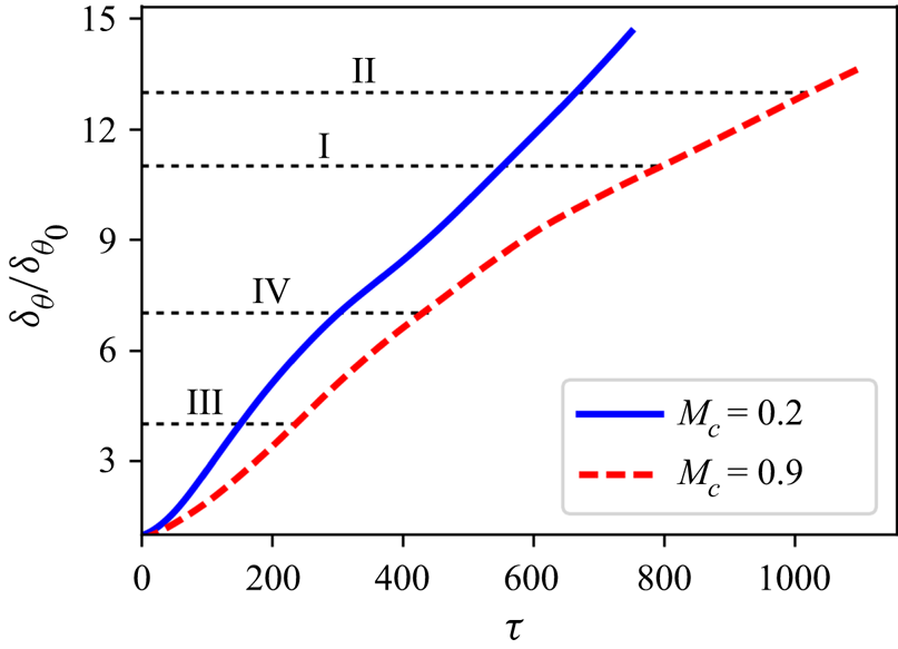
A well-known effect of compressibility on the mixing layer evolution is the suppression of the mixing layer growth rate. This is evident from the momentum thickness evolution, as shown in figure 1. The momentum thickness increases with time and after an initial transient period,  $\delta _\theta$ evolves linearly with time. The asymptotic evolution is characterized by self-similarity of the turbulence statistics such as kinetic energy and Reynolds stress components. Compressibility not only suppresses the linear growth rate but also delays the onset of the self-similar evolution. We examine the energy density function, production and pressure dilatation at different instants when
 $\delta _\theta$ are nearly identical for both Mach numbers, which is indicated by the horizontal dotted lines in figure 1.
Evolution of mixing layer momentum thickness with non-dimensional time,  $\tau =t\Delta U/\delta _\theta$, for the two cases.

3.1. Scale-space energy density function
The energy density and its budget vary in the transverse direction and its variation is of much interest. We examine the energy density in transverse scales i.e. when the separation vector  $\boldsymbol {r}$ is along
 $x_2$, the inhomogeneous direction. We compare the two-point behaviour in transverse direction with the centreline of the mixing layer serving as the reference (origin) location. Because the flow is statistically symmetric about the centreline, we report the energy density and budgets for
 $r_2>0$. The statistics are obtained by averaging in the homogeneous directions. The energy density function,
 $E(r_2)$, is normalized by the local turbulent kinetic energy
 $(K)$ and the Taylor microscale
 $(\lambda )$. As mentioned before, we investigate
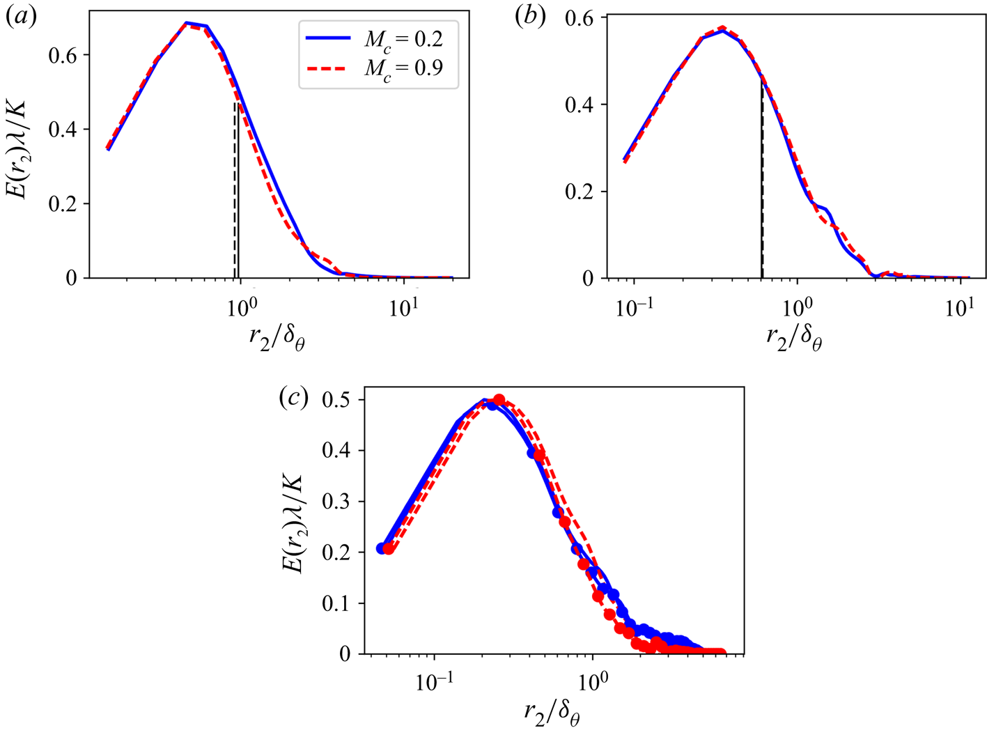
 $E(r_2)$ at different instants, which correspond to the dotted horizontal lines in figure 1, when
 $\delta _\theta$ are nearly identical for both
 $M_c$. The scale-space energy density function at these instants are compared in figure 2. This figure demonstrates that the compressibility effects on two-point statistics at different Mach numbers scale reasonably well with the momentum thickness during transient evolution and asymptotic state. Other scalings do not exhibit such close collapse of statistics during the transient evolution for different Mach numbers.
Normalized scale-space energy density function at instants when momentum thicknesses are nearly identical for the two cases, (a)  $\delta _\theta /\delta _{\theta _0}=4$, (b)
 $\delta _\theta /\delta _{\theta _0}=7$ and (c) during self-similar evolution. In figure (c), the curves without markers correspond to
 $\delta _\theta /\delta _{\theta _0}=11$ and those with circles are for
 $\delta _\theta /\delta _{\theta _0}=13$. The solid and dashed vertical lines in (a,b) represent the Taylor microscale for
 $M_c=0.2$ and
 $M_c=0.9$, respectively.

The relationship between scale-space energy density function and spectral density function was examined by Hamba (Reference Hamba2015). It was shown that the energy content at large scales in spectral space corresponds to the energy density function being high at lower separation distances. As the scale size increases from the smallest scale,  $E({r_2})$ increases, reaches a peak and then decays to zero with the peak occurring at a scale size smaller than the Taylor-length scale. The energy distribution over a range of scales is given by (2.3), where the limits of the integral are the bounds of the specified range. This way, the scales smaller than the Taylor scale, shown by means of the solid and dashed vertical lines in figures 2(a) and 2(b), are found to account for one-third of the turbulent kinetic energy whereas the larger scales contain twice as much energy at both
 $M_c$. The energy density decays to zero when
 $r_2/\delta _\theta \gg 1$ and turbulent kinetic energy is almost entirely distributed among scales of size smaller than the vorticity thickness,
 $\delta _\omega \approx 4\delta _\theta$.
The findings indicate that the normalized scale-space energy density function evolution is reasonably independent of Mach number. All of the compressibility effects manifest via the momentum thickness reduction and suppression of turbulent kinetic energy. Furthermore, the asymptotic state is identical at different Mach numbers.
3.2. Production and pressure dilatation
We analyse some of the key scale-space transport terms in (2.19) using the DNS data. Two important terms – production of energy density and pressure-dilatation effects – at the centreline of the mixing layer are analysed during the self-similar evolution. As with the energy density function, the transport terms are normalized by the turbulent kinetic energy at the centreline and the Taylor microscale.
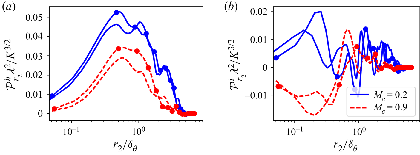
The homogeneous and inhomogeneous parts of the production of the energy density function given by (2.20) are shown in figure 3. The first part is the production arising from mean shear which, on integration over the scale space, yields the production term in the single-point turbulent kinetic energy transport equation. These contributions for the two Mach numbers at two different instants during their self-similar evolution are shown in the figure. The homogeneous part, shown in figure 3(a), is positive for the entire range of scales and decays to zero for separation distances larger than the vorticity thickness. This implies that the extraction of energy from the mean flow to turbulence by mean shear is influenced by scales as large as the vorticity thickness. However, as seen in figure 3(b), inhomogeneous production exhibits temporal variations, which implies a dynamic equilibrium behaviour even at the asymptotic state. Integration of this contribution over the scale space yields zero as the process is a scale-space phenomenon which only transfers energy across the scales. Again, it is evident that the inhomogeneous production is non-zero for scales up to vorticity thickness.
(a) Homogeneous and (b) inhomogeneous parts of the production of energy density owing to mean shear. Curves without markers correspond to  $\delta _\theta /\delta _{\theta _0}=11$ and those with circles are for
 $\delta _\theta /\delta _{\theta _0}=13$.

Another key scale-space transport term, from the perspective of compressibility effects in mixing layers, is the pressure dilatation contribution,  $\varPi _{r_\alpha }$. The integral of
 $\varPi _{r_\alpha }$ over the scale space gives the pressure dilatation term in the turbulent kinetic energy transport equation. This term represents an energy transfer path between the kinetic energy and internal energy in compressible turbulent flows. The variation of
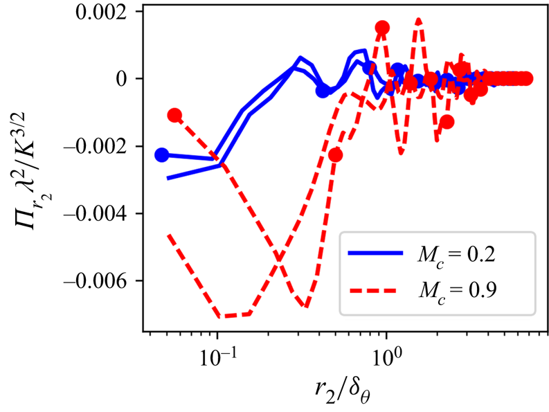
 $\varPi _{r_\alpha }$ with separation distance is shown in figure 4. The term is more relevant at
 $M_c=0.9$, as evident from the larger magnitudes. For small separation distances, the pressure-dilatation correlation extracts energy from the kinetic mode and deposits it into the internal mode. The pressure-dilatation effects are significant at small
 $r_2$ and decay to very small values for separation distances larger than the momentum thickness. This indicates that
 $\varPi _{r_\alpha }$ is more a local phenomenon in comparison with the energy density production which acts over the range of separation distances as large as the vorticity thickness. Furthermore,
 $\varPi _{r_\alpha }$ takes both positive and negative values, which suggests that the pressure-dilatation term affects the energy transfer across scales in addition to that between kinetic and internal energy modes.
Contribution from pressure dilatation effects to energy density transport at the centreline of the mixing layer. Curves without markers correspond to  $\delta _\theta /\delta _{\theta _0}=11$ and those with circles are for
 $\delta _\theta /\delta _{\theta _0}=13$.

Analysis of DNS data using the scale-space energy density function and its scale-space transport equation provides insight into the scale-space dynamics which cannot be studied using spectral methods and Fourier analyses. The analysis reveals the distribution of energy across the different scales of motion as well as the influence of the separation distance. A more in-depth analysis of the other scale-space transport terms, such as dissipation, interscale transfer and dilatation terms in (2.19), and comparison with similar processes in spectral energy transfer will be covered in a subsequent article.
4. Summary and conclusion
The scale-space energy density function  $E(\boldsymbol {x},\boldsymbol {r})$ describes the energy intensity in different scales (
 $\boldsymbol {r}$) of turbulent motion at various locations (
 $\boldsymbol {x}$) in the flow field. The function
 $E(\boldsymbol {x},\boldsymbol {r})$ not only extends the concept of spectral energy density distribution to inhomogeneous flows, but also describes detailed energy interactions between any two locations in the flow field. In this work, the transport equations for
 $E(\boldsymbol {x},\boldsymbol {r})$ in variable-density and compressible flows are developed. In the limit of vanishing dilatation and uniform density, the new transport equation simplifies to that derived by Hamba (Reference Hamba2015) for incompressible flows. In homogeneous turbulence, the present equation is consistent with the spectral energy density equation of Praturi & Girimaji (Reference Praturi and Girimaji2019).
The integral of the  $E(\boldsymbol {x},\boldsymbol {r})$ transport equation over the entire range of scales yields the turbulent kinetic energy budget equation at a given spatial location. The analysis provides valuable insight into the scale distribution and degree of non-locality of compressibility effects on energy production, dissipation and turbulent transport. The equations describing the evolution of the scale-space energy density function are used to analyse compressible mixing layers at different convective Mach numbers using DNS data. The variation of energy density and different transport terms across the scales are studied. The energy density function for the different Mach numbers are collapsed by suitable scaling with the local turbulent kinetic energy and Taylor microscale. The energy density production and pressure-dilatation effects at different scales are also analysed. The energy density production is found to be influenced by scales as large as
 $\delta _\omega$, whereas the pressure-dilatation effects are more local. The analysis of DNS data demonstrates the potential of the scale-space energy density function and scale-space transport terms to account for the relative importance of various physical processes at different separation distances.
The analysis developed in the study will serve as the foundation for examining the influence of shocks, chemical reaction (combustion), compression/expansion waves and dilatational flow structures on scale-to-scale energy transfer and non-locality effects in inhomogeneous high-Mach-number turbulent flows. Filtering the scale-space energy density function along the lines of that done by Hamba (Reference Hamba2018) can lead to the development of advanced cut-off dependent closure models for practical flow computations.
Acknowledgements
The authors thank T.T. Clark for the fruitful discussions during the course of this work. Authors thank SPARC from the Govt. of India for funding of the project. The computational resources are provided by the High Performance Computing Environment Facility at IIT Madras.
Declaration of interests
The authors report no conflict of interest.
Appendix A. Detailed derivation of the transport equation
The instantaneous velocity field for compressible flow is given by the Navier–Stokes equation of the form
 \begin{equation} \frac{\partial{\rho u_i}}{\partial {t}}+\frac{\partial{\rho u_iu_k}}{\partial {x_k}}=\frac{\partial{\sigma_{ik}}}{\partial {x_k}}, \end{equation}
where  $\sigma _{ik}=-p\delta _{ik}+\tau _{ik}$ and
 \begin{equation} \tau_{ik}=\mu\left({\frac{\partial{u_i}}{\partial {x_k}}+\frac{\partial{u_k}}{\partial {x_i}}-\frac{2}{3}\frac{\partial{u_m}}{\partial {x_m}}\delta_{ik}}\right). \end{equation}
The mass conservation equation is
 \begin{equation} \frac{\partial{\rho}}{\partial {t}}+\frac{\partial{\rho u_k}}{\partial {x_k}}=0. \end{equation}
From (A1) and (A3), the exact equation for instantaneous velocity is given by
 \begin{equation} \frac{\partial{u_i}}{\partial {t}}+u_k\frac{\partial{u_i}}{\partial {x_k}}=\frac{1}{\rho}\frac{\partial{\sigma_{ik}}}{\partial {x_k}}. \end{equation}
Applying Favre-averaging to the momentum and mass conservation equations,
 $$\begin{gather} \frac{\partial{\bar{\rho}\tilde{u}_i}}{\partial {t}}+\frac{\partial{\bar{\rho}\tilde{u}_i\tilde{u}_k}}{\partial {x_k}}+\frac{\partial{R_{ik}}}{\partial {x_k}}=\frac{\partial{\bar{\sigma}_{ik}}}{\partial {x_k}}, \end{gather}$$
 $$\begin{gather}\frac{\partial{\bar{\rho}}}{\partial {t}}+\frac{\partial{\bar{\rho}\tilde{u}_k}}{\partial {x_k}}=0, \end{gather}$$
where  $R_{ik}=\overline {\rho u''_iu''_k}$ is the turbulent stress. From these, an exact equation for
 $\tilde {u}_i$ is obtained as
 \begin{equation} \frac{\partial{\tilde{u}_i}}{\partial {t}}+\tilde{u}_k\frac{\partial{\tilde{u}_i}}{\partial {x_k}}+\frac{1}{\bar{\rho}}\frac{\partial{R_{ik}}}{\partial {x_k}}=\frac{1}{\bar{\rho}}\frac{\partial{\bar{\sigma}_{ik}}}{\partial {x_k}}. \end{equation}
The equation for fluctuating velocity is then obtained by subtracting (A7) from (A4),
 \begin{equation} \frac{\partial{u''_i}}{\partial {t}}+\underbrace{u_k\frac{\partial{u''_i}}{\partial {x_k}}+u''_k\frac{\partial{\tilde{u}_i}}{\partial {x_k}}}_{I}-\frac{1}{\bar{\rho}}\frac{\partial{R_{ik}}}{\partial {x_k}} = \frac{1}{\rho}\frac{\partial{\sigma'_{ik}}}{\partial {x_k}}+\left({{v}-\frac{1}{\bar{\rho}}}\right)\frac{\partial{\bar{\sigma}_{ik}}}{\partial {x_k}}, \end{equation}
where  $ {v}=1/\rho$ is the specific volume. This equation can be rewritten in the conservative form, by making use of (A3), as
 \begin{equation} \frac{\partial{\rho u''_i}}{\partial {t}}+\underbrace{\frac{\partial{\rho u''_iu_k}}{\partial {x_k}}+\rho u''_k\frac{\partial{\tilde{u}_i}}{\partial {x_k}}}_{II}-\frac{\rho}{\bar{\rho}}\frac{\partial{R_{ik}}}{\partial {x_k}} = \frac{\partial{\sigma'_{ik}}}{\partial {x_k}}+\left({1-\frac{\rho}{\bar{\rho}}}\right)\frac{\partial{\bar{\sigma}_{ik}}}{\partial {x_k}}. \end{equation}
A.1. Transport equation for two-point correlation
To derive the two-point correlation transport equation, we consider two points  $x_1$ and
 $x_2$, where in the main text,
 $\boldsymbol {x}$ and
 $\boldsymbol {x}'$, respectively, denote these spatial locations. The two-point correlation is defined as
 \begin{equation} Q_{ij}\left({x_1,x_2}\right)=\tfrac{1}{2}\overline{\left[\rho(x_1)+\rho(x_2)\right]u''_i(x_1)u''_j(x_2)}. \end{equation}
The time derivative of the unaveraged product is
 \begin{align} \frac{1}{2}\frac{\partial{\left({\rho(x_1)+\rho(x_2)}\right)u''_i(x_1)u''_j(x_2)}}{\partial {t}} &= \frac{1}{2}\frac{\partial{\rho(x_2)u''_j(x_2)u''_i(x_1)}}{\partial {t}}+\frac{1}{2}\frac{\partial{\rho(x_1)u''_i(x_1)u''_j(x_2)}}{\partial {t}} \nonumber\\ &=\frac{\rho(x_2)u''_j(x_2)}{2}\frac{\partial{u''_i(x_1)}}{\partial {t}}+\frac{u''_i(x_1)}{2}\frac{\partial{\rho(x_2)u''_j(x_2)}}{\partial {t}}\nonumber\\ &\quad +\frac{\rho(x_1)u''_i(x_1)}{2}\frac{\partial{u''_{j}(x_2)}}{\partial {t}}+\frac{u''_j(x_2)}{2}\frac{\partial{\rho(x_1)u''_i(x_1)}}{\partial {t}}. \end{align}
Therefore, an exact equation for the two-point correlation is obtained from the conservative and primitive forms of the fluctuating velocity equations at  $x_1$ and
 $x_2$. Performing the same operations as in (A11) on the terms featuring spatial derivatives of velocity on the left-hand sides of (A8) and (A9), specifically terms
 $I$ and
 $II$, yields
 \begin{align} &\frac{\rho(x_2)u''_j(x_2)}{2}I\left(x_1\right)+\frac{u''_i(x_1)}{2}II\left(x_2\right)+\frac{\rho(x_1)u''_i(x_1)}{2}I\left(x_2\right)+\frac{u''_j(x_2)}{2}II\left(x_1\right)\nonumber\\ &\quad =\frac{\rho(x_2)u''_j(x_2)}{2}\left[{u_k\left(x_1\right)\frac{\partial{u''_i(x_1)}}{\partial {x_{k_1}}}+u''_k\left(x_1\right)\frac{\partial{\tilde{u}_i\left(x_1\right)}}{\partial {x_{k_1}}}}\right] \nonumber\\ &\qquad +\frac{u''_i(x_1)}{2}\left[{\frac{\partial{\rho(x_2)u''_j(x_2)u_k\left(x_2\right)}}{\partial {x_{k_2}}}+\rho\left(x_2\right) u''_k\left(x_2\right)\frac{\partial{\tilde{u}_j\left(x_2\right)}}{\partial {x_{k_2}}}}\right]\nonumber\\ &\qquad +\frac{\rho(x_1)u''_i(x_1)}{2}\left[{u_k\left(x_2\right)\frac{\partial{u''_j(x_2)}}{\partial {x_{k_2}}}+u''_k\left(x_2\right)\frac{\partial{\tilde{u}_i\left(x_2\right)}}{\partial {x_{k_2}}}}\right] \nonumber\\ &\qquad +\frac{u''_j(x_2)}{2}\left[{\frac{\partial{\rho(x_1)u''_i(x_1)u_k\left(x_1\right)}}{\partial {x_{k_1}}}+\rho\left(x_1\right) u''_k\left(x_1\right)\frac{\partial{\tilde{u}_i\left(x_1\right)}}{\partial {x_{k_1}}}}\right]. \end{align}
The spatial derivatives at  $x_1$ and
 $x_2$ locations are denoted by subscripts 1 or 2 in the denominator. Each of these terms, as they appear in the transport equation for
 $Q_{ij}(x_1,x_2)$ (Clark Reference Clark2020), is discussed below.
Terms featuring  $\tilde {u}_k(x_1)$ on averaging (A12):
 \begin{align} &\frac{1}{2}\overline{\rho(x_2)u''_j(x_2)\tilde{u}_k\left(x_1\right)\frac{\partial{u''_i\left(x_1\right)}}{\partial {x_{k_1}}}}+\frac{1}{2}\overline{u''_{j}(x_2)\frac{\partial{\rho\left(x_1\right) u''_i\left(x_1\right)\tilde{u}_k\left(x_1\right)}}{\partial {x_{k_1}}}} \nonumber\\ &\quad =\frac{1}{2}\overline{\frac{\partial{\rho(x_2)u''_j(x_2)u''_i\left(x_1\right)\tilde{u}_k\left(x_1\right)}}{\partial {x_{k_1}}}} +\frac{1}{2}\overline{\frac{\partial{\rho\left(x_1\right) u''_j(x_2)u''_i\left(x_1\right)\tilde{u}_k\left(x_1\right)}}{\partial {x_{k_1}}}}\nonumber\\ &\qquad -\frac{1}{2}\overline{\rho(x_2)u''_i\left(x_1\right) u''_j(x_2)}\frac{\partial{\tilde{u}_k\left(x_1\right)}}{\partial {x_{k_1}}} \nonumber\\ &\quad= \frac{\partial{Q_{ij}(x_1,x_2)\tilde{u}_k\left(x_1\right)}}{\partial {x_{k_1}}}-\frac{1}{2}\overline{\rho(x_2)u''_i\left(x_1\right) u''_j(x_2)}\frac{\partial{\tilde{u}_k\left(x_1\right)}}{\partial {x_{k_1}}}. \end{align}
The terms with  $\tilde {u}_k\left (x_2\right )$ from (A12) also reduce to a similar form, and collecting the terms with minus sign from these,
 \begin{align} &\frac{1}{2}\overline{\rho\left(x_2\right) u''_i\left(x_1\right) u''_j\left(x_2\right)}\frac{\partial{\tilde{u}_k\left(x_1\right)}}{\partial {x_{k_1}}}+\frac{1}{2}\overline{\rho\left(x_1\right) u''_j\left(x_2\right) u''_i\left(x_1\right)}\frac{\partial{\tilde{u}_k\left(x_2\right)}}{\partial {x_{k_2}}}\nonumber\\ &\quad = \frac{1}{2}\overline{\left[{\rho\left(x_2\right)-\frac{\rho\left(x_1\right)}{2}+\frac{\rho\left(x_1\right)}{2}}\right]u''_i\left(x_1\right) u''_j}\left(x_2\right)\frac{\partial{\tilde{u}_k\left(x_1\right)}}{\partial {x_{k_1}}}\nonumber\\ &\qquad + \frac{1}{2}\overline{\left[{\rho\left(x_1\right)-\frac{\rho\left(x_2\right)}{2}+\frac{\rho\left(x_2\right)}{2}}\right] u''_j\left(x_2\right) u''_i\left(x_1\right)}\frac{\partial{\tilde{u}_k\left(x_2\right)}}{\partial {x_{k_2}}}\nonumber\\ &\quad = \frac{1}{4}\overline{\left[{\rho\left(x_1\right)+\rho\left(x_2\right)}\right]u''_i\left(x_1\right) u''_j\left(x_2\right)}\frac{\partial{\tilde{u}_k\left(x_1\right)}}{\partial {x_{k_1}}}\nonumber\\ &\qquad+\frac{1}{4}\overline{\left[{\rho\left(x_1\right)+\rho\left(x_2\right)}\right]u''_i\left(x_1\right) u''_j\left(x_2\right)}\frac{\partial{\tilde{u}_k\left(x_2\right)}}{\partial {x_{k_2}}} \nonumber\\ &\qquad -\frac{1}{4}\overline{\left[{\rho\left(x_2\right)-\rho\left(x_1\right)}\right]u''_i\left(x_1\right) u''_j\left(x_2\right)}\frac{\partial{\tilde{u}_k\left(x_1\right)}}{\partial {x_{k_1}}}\nonumber\\ &\qquad +\frac{1}{4}\overline{\left[{\rho\left(x_1\right)-\rho\left(x_2\right)}\right]u''_i\left(x_1\right) u''_j\left(x_2\right)}\frac{\partial{\tilde{u}_k\left(x_2\right)}}{\partial {x_{k_2}}}\nonumber\\ &\quad = \frac{1}{2}Q_{ij}(x_1,x_2)\left[\frac{\partial{\tilde{u}_k\left(x_1\right)}}{\partial {x_{k_1}}}+\frac{\partial{\tilde{u}_k\left(x_2\right)}}{\partial {x_{k_2}}}\right]\nonumber\\ &\qquad + \frac{1}{2}Q_{ij}^{(-)}(x_1,x_2)\left[\frac{\partial{\tilde{u}_k\left(x_2\right)}}{\partial {x_{k_2}}}-\frac{\partial{\tilde{u}_k\left(x_1\right)}}{\partial {x_{k_1}}}\right] , \end{align}
where  $Q_{ij}^{(-)}\left ({x_1,x_2}\right )=(\overline {\left [{\rho \left (x_1\right )-\rho \left (x_2\right )}\right ]u''_i\left (x_1\right ) u''_j\left (x_2\right )})/{2}$.
Terms featuring  $\tilde {u}_i(x_1)$ and
 $\tilde {u}_j(x_2)$ from (A12):
 $$\begin{gather} \frac{1}{2}\overline{\rho\left(x_2\right) u''_j\left(x_2\right) u''_k\left(x_1\right)}\frac{\partial{\tilde{u}_i\left(x_1\right)}}{\partial {x_{k_1}}}+\frac{1}{2} \overline{u''_j\left(x_2\right)\rho\left(x_1\right) u''_k\left(x_1\right)}\frac{\partial{\tilde{u}_i\left(x_1\right)}}{\partial {x_{k_1}}}=Q_{kj}(x_1,x_2)\frac{\partial{\tilde{u}_i\left(x_1\right)}}{\partial {x_{k_1}}} \end{gather}$$
 $$\begin{gather}\frac{1}{2}\overline{\rho\left(x_1\right) u''_i\left(x_1\right) u''_k\left(x_2\right)}\frac{\partial{\tilde{u}_j\left(x_2\right)}}{\partial {x_{k_2}}}+\frac{1}{2}\overline{u''_i\left(x_1\right)\rho\left(x_2\right) u''_k\left(x_2\right)}\frac{\partial{\tilde{u}_j\left(x_2\right)}}{\partial {x_{k_2}}}=Q_{ki}(x_1,x_2)\frac{\partial{\tilde{u}_j\left(x_2\right)}}{\partial {x_{k_2}}}. \end{gather}$$
Triple correlation terms on averaging terms with derivatives of  $u''_i\left (x_1\right )$ in (A12):
 \begin{align} &\frac{1}{2}\overline{\rho(x_2)u''_j(x_2)u''_k(x_1)\frac{\partial{u''_i(x_1)}}{\partial {x_{k_1}}}}+\frac{1}{2}\overline{u''_j(x_2)\frac{\partial{\rho(x_1)u''_i(x_1)u''_k(x_1)}}{\partial {x_{k_1}}}}\nonumber\\ &\quad =\frac{1}{2}\overline{\frac{\partial{\rho(x_2)u''_j(x_2)u''_i(x_1)u''_k(x_1)}}{\partial {x_{k_1}}}}+ \frac{1}{2}\overline{\frac{\partial{\rho(x_1)u''_i(x_1)u''_j(x_2)u''_k(x_1)}}{\partial {x_{k_1}}}} \nonumber\\ &\qquad -\frac{1}{2}\overline{\rho(x_2)u''_j(x_2)u''_i(x_1)\frac{\partial{u''_k(x_1)}}{\partial {x_{k_1}}}}\nonumber\\ &\quad =\frac{1}{2}\frac{\partial{}}{\partial {x_{k_1}}}\overline{\left[{\rho\left(x_1\right)+\rho\left(x_2\right)}\right]u''_i\left(x_1\right) u''_j\left(x_2\right) u''_k\left(x_1\right)}-\frac{1}{2}\overline{\rho(x_2)u''_j(x_2)u''_i(x_1)\frac{\partial{u''_k(x_1)}}{\partial {x_{k_1}}}}. \end{align}
Two terms similar to (A17) are obtained from the spatial derivatives of  $u''\left (x_2\right )$ in (A12). Collecting the terms featuring fluctuating field dilatation from (A17) and its similar form,
 \begin{equation} \zeta_{ij}\left({x_1,x_2}\right)=\frac{1}{2}\overline{\rho\left(x_2\right) u''_i\left(x_1\right) u''_j\left(x_2\right)\frac{\partial{u''_k\left(x_1\right)}}{\partial {x_{k_1}}}}+\frac{1}{2}\overline{\rho\left(x_1\right) u''_i\left(x_1\right) u''_j\left(x_2\right)\frac{\partial{u''_k\left(x_2\right)}}{\partial {x_{k_2}}}}. \end{equation}
Fluctuating stress terms in (A8) and (A9) give
 \begin{align} &\frac{1}{2}\overline{\rho(x_2)u''_j(x_2){v}(x_1)\frac{\partial{\sigma'_{ik}(x_1)}}{\partial {x_{k_1}}}}+\frac{1}{2}\overline{u''_j(x_2)\frac{\partial{\sigma'_{ik}(x_1)}}{\partial {x_{k_1}}}}\nonumber\\ &\quad =\frac{1}{2}\overline{u''_j(x_2)\left[{1+\frac{\rho(x_2)}{\rho(x_1)}}\right]\frac{\partial{\sigma'_{ik}(x_1)}}{\partial {x_{k_1}}}} =\frac{1}{2}\varPsi_{ji}(x_2,x_1). \end{align}
Then, by noting that  $x_2=x_1+r$, the derivatives can be written as (F. Hamba, private communication, April 2018),
 \begin{equation} \frac{\partial{u''_j\left(x_2\right)}}{\partial {x_{k_2}}}=\frac{\partial{u''_j\left({x_1+r}\right)}}{\partial {r_k}}=\frac{\partial{u''_j\left(x_2\right)}}{\partial {x_{k_1}}}. \end{equation}
Therefore,  $\varPsi _{ji}(x_2,x_1)$ can be written as
 \begin{align} \varPsi_{ji}\left({x_2,x_1}\right)&=\overline{\left[{1+\frac{\rho(x_2)}{\rho(x_1)}}\right]\frac{\partial{}}{\partial {x_{k_1}}}u''_j\left(x_2\right)\sigma'_{ik}\left(x_1\right)}-\overline{\left[{1+\frac{\rho(x_2)}{\rho(x_1)}}\right]\sigma'_{ik}\left(x_1\right)\frac{\partial{u''_j\left(x_2\right)}}{\partial {x_{k_2}}}} \nonumber\\ &=\underbrace{\overline{\left[{1+\frac{\rho(x_2)}{\rho(x_1)}}\right]\frac{\partial{}}{\partial {x_{k_1}}}u''_j\left(x_2\right)\tau'_{ik}\left(x_1\right)}}_{\phi_{ij}^\nu(x_2,x_1)} \underbrace{-\overline{\left[{1+\frac{\rho(x_2)}{\rho(x_1)}}\right]\tau'_{ik}\left(x_1\right)\frac{\partial{u''_j\left(x_2\right)}}{\partial {x_{k_2}}}}}_{\psi_{ij}^\nu(x_2,x_1)} \nonumber\\ &\underbrace{-\overline{\left[{1+\frac{\rho(x_2)}{\rho(x_1)}}\right]\frac{\partial{}}{\partial {x_{i_1}}}u''_j\left(x_2\right) p'\left(x_1\right)}}_{\phi_{ij}^p(x_2,x_1)} +\underbrace{\overline{\left[{1+\frac{\rho(x_2)}{\rho(x_1)}}\right]p'\left(x_1\right)\frac{\partial{u''_j\left(x_2\right)}}{\partial {x_{i_2}}}}}_{\psi_{ij}^p(x_2,x_1)}. \end{align}
Coefficients of mean stress gradient  $\bar {\sigma }$ from the primitive (A8) and conservative (A9) forms on averaging give
 \begin{align} &-\frac{1}{2}\overline{\rho\left(x_2\right) u''_j\left(x_2\right)\left({{v}\left(x_1\right)-\frac{1}{\bar{\rho}\left(x_1\right)}}\right)}-\frac{1}{2}\overline{u''_j\left(x_2\right)\left({1-\frac{\rho\left(x_1\right)}{\bar{\rho}\left(x_1\right)}}\right)} \nonumber\\ &\quad ={-}\frac{1}{2}\overline{\left[{\rho\left(x_1\right)+\rho\left(x_2\right)}\right]u''_j\left(x_2\right)\left({{v}\left(x_1\right)-\frac{1}{\bar{\rho}\left(x_1\right)}}\right)} \nonumber\\ &\quad ={-}\frac{1}{2}\overline{\rho\left(x_2\right) u''_j\left(x_2\right){v}\left(x_1\right)}-\frac{1}{2}\overline{u''_j\left(x_2\right)}+\frac{1}{2}\frac{\overline{\rho\left(x_1\right) u''_j\left(x_2\right)}}{\bar{\rho}\left(x_1\right)}=a_j\left({x_2,x_1}\right). \end{align}
Similarly, coefficients of turbulent stress in (A8) and (A9) become
 \begin{equation} -\frac{1}{2}\overline{\rho\left(x_2\right) u''_j\left(x_2\right)}/\bar{\rho}\left(x_1\right)-\frac{1}{2}\overline{\rho\left(x_1\right) u''_j\left(x_2\right)}/\bar{\rho}\left(x_1\right)={-}\frac{1}{2}\frac{\overline{\rho\left(x_1\right) u''_j\left(x_2\right)}}{\bar{\rho}\left(x_1\right)}. \end{equation}
Then, by applying a coordinate transformation,
 \begin{equation} \left.\begin{gathered} x_1=\boldsymbol{x}, \quad x_2=\boldsymbol{x}+\boldsymbol{r}, \\ \frac{\partial{}}{\partial {x_{k_1}}}=\frac{\partial{}}{\partial {x_k}}-\frac{\partial{}}{\partial {r_k}}, \quad \frac{\partial{}}{\partial {x_{k_2}}}=\frac{\partial{}}{\partial {r_k}}, \end{gathered}\right\} \end{equation}
along with the relations (A20), the exact equation for two-point correlation ((2.9) in the main article) is obtained as
 \begin{align}
&\frac{\partial{Q_{ij}(\boldsymbol{x},\boldsymbol{r})}}{\partial
{t}}+\frac{\partial{Q_{ij}(\boldsymbol{x},\boldsymbol{r})\tilde{u}_k(\boldsymbol{x})}}{\partial
{x_{k}}}\nonumber\\ &\quad =
\underbrace{-Q_{kj}(\boldsymbol{x},\boldsymbol{r})\frac{\partial{\tilde{u}_i(\boldsymbol{x})}}{\partial
{x_{k}}}-Q_{ik}(\boldsymbol{x},\boldsymbol{r})\frac{\partial{\tilde{u}_j(\boldsymbol{x}+\boldsymbol{r})}}{\partial
{x_{k}}}}_{\mathcal{P}_{ij}} \nonumber\\
&\qquad\underbrace{-\frac{\partial{T_{ijk}(\boldsymbol{x},\boldsymbol{r})}}{\partial
{x_{k}}}}_{\mathcal{D}^u_{ij}}\notag\\ &\qquad +\underbrace{\frac{1}{2}\left[{\varPhi_{ij}^p(\boldsymbol{x},\boldsymbol{x}+\boldsymbol{r})+\varPhi_{ji}^p(\boldsymbol{x}+\boldsymbol{r},\boldsymbol{x})}\right]}_{\mathcal{D}_{ij}^p}+\underbrace{\frac{1}{2}\left[{\varPhi_{ij}^\nu(\boldsymbol{x},\boldsymbol{x}+\boldsymbol{r})+\varPhi_{ji}^\nu(\boldsymbol{x}+\boldsymbol{r},\boldsymbol{x})}\right]}_{\mathcal{D}_{ij}^\nu}
\nonumber\\ &\qquad
+\underbrace{\frac{1}{2}\left[{\varPsi_{ij}^p(\boldsymbol{x},\boldsymbol{x}+\boldsymbol{r})+\varPsi_{ji}^p(\boldsymbol{x}+\boldsymbol{r},\boldsymbol{x})}\right]}_{\varPi_{ij}}+\underbrace{\frac{1}{2}\left[{\varPsi_{ij}^\nu(\boldsymbol{x},\boldsymbol{x}+\boldsymbol{r})+\varPsi_{ji}^\nu(\boldsymbol{x}+\boldsymbol{r},\boldsymbol{x})}\right]}_{\epsilon_{ij}}
\nonumber\\
&\qquad\underbrace{+\frac{1}{2}Q_{ij}(\boldsymbol{x},\boldsymbol{r})\left[{\frac{\partial{\tilde{u}_k(\boldsymbol{x})}}{\partial
{x_{k}}}+\frac{\partial{\tilde{u}_k(\boldsymbol{x}+\boldsymbol{r})}}{\partial
{x_{k}}}}\right]}_{\chi_{ij}^+}
\underbrace{+\frac{1}{2}Q^{(-)}_{ij}(\boldsymbol{x},\boldsymbol{r})\left[{\frac{\partial{\tilde{u}_k(\boldsymbol{x}+\boldsymbol{r})}}{\partial
{x_{k}}}-\frac{\partial{\tilde{u}_k(\boldsymbol{x})}}{\partial
{x_{k}}}}\right]}_{\chi_{ij}^-} \nonumber\\
&\qquad\underbrace{+\overline{\rho(\boldsymbol{x}+\boldsymbol{r})u''_i(\boldsymbol{x})u''_j(\boldsymbol{x}+\boldsymbol{r})\frac{\partial{u''_k(\boldsymbol{x})}}{\partial
{x_k}}}+\overline{\rho(\boldsymbol{x})u''_i(\boldsymbol{x})u''_j(\boldsymbol{x}+\boldsymbol{r})\frac{\partial{u''_k(\boldsymbol{x}+\boldsymbol{r})}}{\partial
{x_k}}}}_{\zeta_{ij}} \nonumber\\
&\qquad\underbrace{+\frac{1}{2}\left({a_i(\boldsymbol{x},\boldsymbol{x}+\boldsymbol{r})\frac{\partial{\bar{\sigma}_{jk}(\boldsymbol{x}+\boldsymbol{r})}}{\partial
{x_k}}+a_j(\boldsymbol{x}+\boldsymbol{r},\boldsymbol{x})\frac{\partial{\bar{\sigma}_{ik}(\boldsymbol{x})}}{\partial
{x_k}}}\right)}_{\varSigma_{ij}}\notag\\
&\qquad \underbrace{+\frac{1}{2}\left[{c_{ij}(\boldsymbol{x},\boldsymbol{x}+\boldsymbol{r})+c_{ji}(\boldsymbol{x}+\boldsymbol{r},\boldsymbol{x})}\right]}_{\mathcal{R}_{ij}}
\nonumber\\ &\qquad\underbrace{-\frac{\partial{}}{\partial
{r_{k}}}\left[\begin{array}{c}\dfrac{1}{2}\overline{\left({\rho(\boldsymbol{x})+\rho(\boldsymbol{x}+\boldsymbol{r})}\right)u_i''(\boldsymbol{x})u_j''(\boldsymbol{x}+\boldsymbol{r})(u_k''(\boldsymbol{x}+\boldsymbol{r})-u_k''(\boldsymbol{x}))}\\
+\left({\tilde{u}_k(\boldsymbol{x}+\boldsymbol{r})-\tilde{u}_k(\boldsymbol{x})}\right)Q_{ij}(\boldsymbol{x},\boldsymbol{r})\end{array}\right]}_{\mathcal{T}_{ij}}.
\end{align}
Note that the linear transport in scale space, obtained by the transformation (A24), is as follows.
 \begin{align} &\frac{\partial{}}{\partial {x_{k_1}}}Q_{ij}\left({x_1,x_2}\right)\tilde{u}_k\left(x_1\right)+\frac{\partial{}}{\partial {x_{k_2}}}Q_{ij}\left({x_1,x_2}\right)\tilde{u}_k\left(x_2\right) \nonumber\\ &\quad=\frac{\partial{}}{\partial {x_k}}Q_{ij}\left({\boldsymbol{x},\boldsymbol{r}}\right)\tilde{u}_k(\boldsymbol{x}) +\frac{\partial{}}{\partial {r_k}}Q_{ij}\left({\boldsymbol{x},\boldsymbol{r}}\right)\left[{\tilde{u}_k(\boldsymbol{x}+\boldsymbol{r})-\tilde{u}(\boldsymbol{x})}\right]. \end{align}
Similarly, by applying this transformation on nonlinear triple correlation terms yields the corresponding scale-space energy transfer term.
 \begin{align} &\frac{\partial{}}{\partial {x_{k_1}}}\frac{1}{2}\overline{\left[{\rho\left(x_1\right)+\rho\left(x_2\right)}\right]u''_i\left(x_1\right) u''_j\left(x_2\right) u''_k\left(x_1\right)}\nonumber\\ &\qquad +\frac{\partial{}}{\partial {x_{k_2}}}\frac{1}{2}\overline{\left[{\rho\left(x_1\right)+\rho\left(x_2\right)}\right]u''_i\left(x_1\right) u''_j\left(x_2\right) u''_k\left(x_2\right)}\nonumber\\ &\quad= \frac{\partial{T_{ijk}(\boldsymbol{x},\boldsymbol{r})}}{\partial {x_k}} +\frac{1}{2}\frac{\partial{}}{\partial {r_k}}\overline{\left[{\rho(\boldsymbol{x})+\rho(\boldsymbol{x}+\boldsymbol{r})}\right]u''_i(\boldsymbol{x})u''_j(\boldsymbol{x}+\boldsymbol{r})\left[{u''_k(\boldsymbol{x}+\boldsymbol{r})-u''_k(\boldsymbol{x})}\right]}. \end{align}
By applying product rule to the second term on the left-hand side of (A25),
 \begin{equation} \frac{\partial{Q_{ij}(\boldsymbol{x},\boldsymbol{r})\tilde{u}_k(\boldsymbol{x})}}{\partial {x_k}}=\tilde{u}_k(\boldsymbol{x})\frac{\partial{Q_{ij}(\boldsymbol{x},\boldsymbol{r})}}{\partial {x_k}}+Q_{ij}(\boldsymbol{x},\boldsymbol{r})\frac{\partial{\tilde{u}_k(\boldsymbol{x})}}{\partial {x_k}}. \end{equation}
The second term is then combined with the mean field dilatation terms,  $\chi _{ij}^+$ and
 $\chi _{ij}^-$, in (A25) to redefine
 \begin{align} \chi_{ij}&=\chi_{ij}^+{+}\chi_{ij}^-{-}Q_{ij}(\boldsymbol{x},\boldsymbol{r})\frac{\partial{\tilde{u}_k(\boldsymbol{x})}}{\partial {x_k}}\nonumber\\ &=\frac{1}{2}Q_{ij}(\boldsymbol{x},\boldsymbol{r})\left[{\frac{\partial{\tilde{u}_k(\boldsymbol{x})}}{\partial {x_{k}}}+\frac{\partial{\tilde{u}_k(\boldsymbol{x}+\boldsymbol{r})}}{\partial {x_{k}}}}\right]+\frac{1}{2}Q^{(-)}_{ij}(\boldsymbol{x},\boldsymbol{r})\left[{\frac{\partial{\tilde{u}_k(\boldsymbol{x}+\boldsymbol{r})}}{\partial {x_{k}}}-\frac{\partial{\tilde{u}_k(\boldsymbol{x})}}{\partial {x_{k}}}}\right]\nonumber\\ &\quad-Q_{ij}(\boldsymbol{x},\boldsymbol{r})\frac{\partial{\tilde{u}_k(\boldsymbol{x})}}{\partial {x_k}} \nonumber\\ &=\frac{1}{2}\left[{Q_{ij}(\boldsymbol{x},\boldsymbol{r})+Q_{ij}^{(-)}(\boldsymbol{x},\boldsymbol{r})}\right]\left[{\frac{\partial{\tilde{u}_k(\boldsymbol{x}+\boldsymbol{r})}}{\partial {x_{k}}}-\frac{\partial{\tilde{u}_k(\boldsymbol{x})}}{\partial {x_{k}}}}\right] \nonumber\\ &=\frac{1}{2}\overline{\rho(\boldsymbol{x})u''_i(\boldsymbol{x})u''_j(\boldsymbol{x}+\boldsymbol{r})}\left[{\frac{\partial{\tilde{u}_k(\boldsymbol{x}+\boldsymbol{r})}}{\partial {x_{k}}}-\frac{\partial{\tilde{u}_k(\boldsymbol{x})}}{\partial {x_{k}}}}\right]. \end{align}
Then,  $\chi _{ij}^{(+)}$ and
 $\chi _{ij}^{(-)}$ no longer feature in the transport equation and the respective contributions are accounted in the new form of
 $\chi _{ij}$.
With the transformations (A24) and simplifications of dilatational terms, the trace of the two-point tensor equation (A25) gives the transport equation for  $Q_{ii}(\boldsymbol {x},\boldsymbol {r})$, which is more appropriate, comapred with the form given by Clark (Reference Clark2020), to represent the scale-space dynamics when the scale-space energy density transport is derived from it.
A.2. Energy density budget
The scale-space energy density function is defined as
 \begin{equation} E(\boldsymbol{x},r)={-}\frac{1}{2}\frac{\partial{}}{\partial {r}}Q_{ii}(x,r). \end{equation}
A transport equation for  $E(\boldsymbol {x},r)$ is obtained by performing the operation
 $-({1}/{2})(\partial /\partial r)$ on the trace of (A25). Differentiation with respect to
 $r$ commutes with those in space and time. In the main article, we use
 $r_\alpha$ instead or
 $r$ to denote the scale.
The time derivative term yields
 \begin{equation} -\frac{1}{2}\frac{\partial{}}{\partial {r}}\frac{\partial{Q_{ii}(\boldsymbol{x},\boldsymbol{r})}}{\partial {t}}=\frac{\partial{}}{\partial {t}}\left({-\frac{1}{2}\frac{\partial{}}{\partial {r}}Q_{ii}(\boldsymbol{x},\boldsymbol{r})}\right)=\frac{\partial{E(\boldsymbol{x},\boldsymbol{r})}}{\partial {t}}. \end{equation}
The spatial derivative on the left-hand side of (2.11) yields
 \begin{equation} -\frac{1}{2}\frac{\partial{}}{\partial {r}}\left({\tilde{u}_k(\boldsymbol{x})\frac{\partial{Q_{ii}(\boldsymbol{x},\boldsymbol{r})}}{\partial {x_k}}}\right)=\tilde{u}_k(\boldsymbol{x})\frac{\partial{}}{\partial {r}}\left({-\frac{1}{2}Q_{ii}(\boldsymbol{x},\boldsymbol{r})}\right)=\tilde{u}_k(\boldsymbol{x})\frac{\partial{E(\boldsymbol{x},\boldsymbol{r})}}{\partial {x_k}}. \end{equation}
The mean shear terms on the right-hand side of (2.11) give
 \begin{align} \mathcal{P}_r&={-}\frac{1}{2}\frac{\partial{\mathcal{P}_{ii}}}{\partial {r}}= \frac{1}{2}\frac{\partial{}}{\partial {r}}\left({Q_{ki}(\boldsymbol{x},\boldsymbol{r})\frac{\partial{\tilde{u}_i(\boldsymbol{x})}}{\partial {x_k}}+Q_{ik}(\boldsymbol{x},\boldsymbol{r})\frac{\partial{\tilde{u}_i(\boldsymbol{x}+\boldsymbol{r})}}{\partial {x_k}}}\right)\nonumber\\ &=\frac{1}{2}\frac{\partial{Q_{ki}(\boldsymbol{x},\boldsymbol{r})}}{\partial {r}}\frac{\partial{\tilde{u}_i(\boldsymbol{x})}}{\partial {x_k}}+\frac{1}{2}\frac{\partial{}}{\partial {r}} \left({Q_{ik}(\boldsymbol{x},\boldsymbol{r})\frac{\partial{\tilde{u}_i(\boldsymbol{x}+\boldsymbol{r})}}{\partial {x_k}}}\right)\nonumber\\ &\quad+\frac{1}{2}\frac{\partial{Q_{ik}(\boldsymbol{x},\boldsymbol{r})}}{\partial {r}}\frac{\partial{\tilde{u}_i(\boldsymbol{x})}}{\partial {x_k}}-\frac{1}{2} \frac{\partial{Q_{ik}(\boldsymbol{x},\boldsymbol{r})}}{\partial {r}}\frac{\partial{\tilde{u}_i(\boldsymbol{x})}}{\partial {x_k}} \nonumber\\ &=\frac{1}{2}\frac{\partial{Q_{ki}(\boldsymbol{x},\boldsymbol{r})}}{\partial {r}}\left({\frac{\partial{\tilde{u}_i(\boldsymbol{x})}}{\partial {x_k}}+\frac{\partial{\tilde{u}_k(\boldsymbol{x})}}{\partial {x_i}}}\right) +\frac{1}{2}\frac{\partial{}}{\partial {r}}\left({Q_{ik}(\boldsymbol{x},\boldsymbol{r})\frac{\partial{\left({\tilde{u}_i(\boldsymbol{x}+\boldsymbol{r})-\tilde{u}_i(\boldsymbol{x})}\right)}}{\partial {x_k}}}\right) \end{align}
The other terms in the energy density transport equation (2.19) are expressed as the derivatives of the respective terms in (A25) and require no further manipulations.