Introduction
Precipitation is an important parameter controlling the growth and the shrinking of the Antarctic ice sheets, since it is the dominant term contributing to mass accumulation (King & Turner Reference King and Turner1997). Observational information on precipitation events is scarce due to the difficulties in measuring precipitation under Antarctic conditions, even when using automatic weather stations (AWS). For instance, AWS or snow stakes provide information about accumulation, but the difficulty arises to differentiate between blowing snow, precipitation, sublimation and compaction, and to convert the height of snow into a water equivalent mass without knowing the snow density (see King & Turner (Reference King and Turner1997) and van den Broeke et al. (Reference Van Den Broeke, Reijmer and Van De Wal2004)).
Snow accumulation climatology (e.g. Bromwich Reference Bromwich1988, Vaughan et al. Reference Vaughan, Bamber, Giovinetto, Russell and Cooper1999, Monaghan et al. Reference Monaghan, Bromwich, Fogt, Wang, Mayewski, Dixon, Ekaykin, Frezzotti, Goodwin, Isaksson, Kaspari, Morgan, Oerter, Van der Veen and Wen2006a) is frequently used as an indicator for precipitation climatology. Evaporation is estimated to amount to roughly 12% of the annual mean precipitation for the whole Antarctic ice sheet (King & Turner Reference King and Turner1997). Studies with climate models (e.g. Van Lipzig et al. Reference Van Lipzig, King, Lachlan-Cope and Van Den Broeke2004, Monaghan et al. Reference Monaghan, Bromwich and Wang2006b, Van de Berg et al. Reference Van De Berg, Van Den Broeke, Reijmer and Van Meijgaard2006) have become very valuable to gain information about the spatial and temporal (on the time scale of seasons and years) variability of precipitation.
Horizontal accumulation and precipitation distributions in Antarctica show the largest annual values near the coast and slightly inland, where the steepest slopes are found. At the Dronning Maud Land (DML) coast, annual accumulation can reach 500 mm, but drops rapidly to less than 50 mm further inland for elevations above 3000 m (Bromwich Reference Bromwich1988). Large portions of precipitation in coastal regions fall episodically, caused by cyclonic systems and fronts (King & Turner Reference King and Turner1997). The depressions are usually weak, generating low intensity precipitation. Sometimes, however, more active fronts reach the coastal region and bring moderate to heavy precipitation. Noone et al. (Reference Noone, Turner and Mulvaney1999) found in case studies that the heaviest precipitation events are related to situations characterized by amplified upper level planetary waves and by the presence of a cyclone in the north-eastern Weddell Sea; in such situations, warm and moist air is directed toward the continent at the eastern side of the cyclone. The precipitation distribution following the synoptic pattern is related to the steep coastal topography, which forces air flowing onshore to rise. Thus, precipitation formation is strongly enhanced.
The episodic nature of coastal precipitation is of significance for the interpretation of ice cores taken on the DML plateau, as addressed by Noone et al. (Reference Noone, Turner and Mulvaney1999). If the accumulation profile becomes biased toward particular months with more frequent frontal precipitation, the temperature derived from ice core analysis will likewise be biased. This requires the knowledge of both the amount and the timing of precipitation as well as the investigation of precipitation events on short time scales.
Information about the precipitation distribution during particular weather events can be gained at present only with the help of weather prediction models. Such a modelling system has been developed in the form of the US Antarctic Mesoscale Prediction System (AMPS) for real-time weather forecasting with the Polar MM5 model, see Powers et al. (Reference Powers, Monaghan, Cayette, Bromwich, Kuo and Manning2003), Bromwich et al. (Reference Bromwich, Monaghan, Manning and Powers2005), and Monaghan et al. (Reference Monaghan, Bromwich, Powers and Manning2005). Although particular emphasis is placed on the McMurdo region, forecasts are also available for e.g. DML with a horizontal mesh size of 20 km (http://www.mmm.ucar.edu/rt/mm5/amps).
Observations in limited regions indicate that accumulation rates are highly variable in space. For instance, Rotschky et al. (Reference Rotschky, Eisen, Wilhelms, Nixdorf and Oerter2004) report a complex accumulation pattern superimposed on a field of generally low values on the DML plateau with strong variations on a spatial scale of about 10 km. Such pattern may be investigated by small-scale modelling, which involves considerable computational expense. Even though currently feasible mesh sizes may not be sufficient to resolve structures on the small spatial scales reported by Rotschky et al. (Reference Rotschky, Eisen, Wilhelms, Nixdorf and Oerter2004), model studies with mesh sizes smaller than 20 km might be an acceptable approach.
To that end, we use the non-hydrostatic weather prediction model of the Consortium for Small Scale Modelling, the COSMO Model. This model, formerly named ‘Lokal-Modell’ (LM), is described in Steppeler et al. (Reference Steppeler, Doms and Schättler2003). The COSMO members run this model as an operational weather forecast model. At the Deutscher Wetterdienst (German Meteorological Service) it is used over Europe with a 7 km mesh size for 72 hour forecasts starting at 00 and 12 UTC as well as for 48 hour forecasts starting at 06 and 18 UTC. Over Germany the model also runs with a 2.8 km mesh size for 21 hour forecasts starting every three hours.
The COSMO Model, recently configured for the Weddell Sea and DML region in Antarctica, is applied to special weather episodes covering several days to investigate the spatial variability of precipitation in DML. As a first step, we use the model with a mesh size of 7 km, which allows spatial structures on a scale of some 30 to 40 km and larger to be resolved. It should be noted that models do not necessarily converge at finer resolution, as discussed by Bryan et al. (Reference Bryan, Wyngaard and Fritsch2003) for convection simulations.
A weather situation from February 1999 is selected, in which several low-pressure systems moved southwards and eastwards towards and along the coast of DML, because AWS observations at Kohnen Station indicate a comparatively strong precipitation event (see Fig. 10 in van den Broeke et al. (Reference Van Den Broeke, Reijmer and Van De Wal2004)). This study therefore will serve to evaluate the ability of the COSMO Model in its operational version to cope with Antarctic weather conditions and will yield information about the horizontal variability of precipitation during a particular episode.
Model design and simulation setup
The COSMO Model is a mesoscale limited area model initially developed at the Deutscher Wetterdienst (DWD). It is now operated and further developed by the COSMO members. In addition to operational use at the weather services, it is also applied for various scientific purposes in weather prediction and for regional climate simulations. The COSMO Model is based on the integration of the full set of thermohydrodynamic equations for the moist atmosphere with prognostic equations for horizontal and vertical wind components, pressure perturbation (i.e. deviation from the prescribed hydrostatic reference profile), and mass fractions of water vapour and of several condensate categories. A generalized terrain-following height coordinate and geographic coordinates λ and ϕ are used. The latter are transformed into a rotated coordinate system, in which the pole is placed in such a way to ensure approximately uniform horizontal resolution over the model domain.
To account for the impact of sub-grid scale processes on the prognostic variables, various parameterization packages are implemented. The impact of microphysical processes in clouds, which fill a whole grid volume, is represented in terms of an extended Kessler scheme. We use a version which accounts for condensates in the form of cloud droplets, rain drops, cloud ice crystals and precipitating snowflakes. Each category is characterized by its mass fraction. For all condensate categories the full mass budget equations are solved; note that this also includes the treatment of advection of precipitating particles. In the presence of cloud water, liquid water saturation adjustment is performed.
The reader is referred to Steppeler et al. (Reference Steppeler, Doms and Schättler2003) and the model documentation (Doms & Schättler Reference Doms and Schättler1999, Reference Doms and Schättler2002, Doms et al. Reference Doms, Schättler and Schulz2003) for the parameterized treatment of turbulent vertical exchange, sub-grid scale clouds, moist convection, and radiative transfer as well as for other detailed information on the COSMO Model. The surface fluxes of momentum, heat, and moisture are calculated by a stability and roughness-length dependent formulation according to Louis (Reference Louis1979). Temperature and the specific humidity at the surface are calculated with a two layer soil model. Climatological values are prescribed for a third layer. Details of the soil model are given in the Appendix. The employment of the model for the situation of an Arctic cold air outbreak is described in Wacker et al. (Reference Wacker, Potty, Lüpkes, Hartmann and Raschendorfer2005).
The weather episode from February 1999 is investigated using Version 3.15 of the COSMO Model. A sequence of 48 hour simulation runs were performed, starting at 12 UTC at each day from 1–11 February.
Various parts of the forecast run used in the present analysis are specified in relevant sections of the text. In particular, vertically integrated cloud condensate contents and precipitation sums will be discussed for various discarded spin-up periods. The model domain extends over more than 2000 km x 2000 km in the zonal and meridional directions from north of the Weddell Sea to the DML plateau. The horizontal grid spacing in the rotated grid is chosen as Δλ = Δϕ = 0.0625°, corresponding to a mesh length of approximately 7 km. We have 301 gridpoints in the south–north and 321 gridpoints in the east–west direction. The atmosphere is vertically divided into 35 layers of unequal thickness with 10 layers in the lowest 1500 m. The top of the model is placed at a pressure of 20 hPa, a height of some 25.6 km. The time step is 20 s. Initial and boundary data are interpolated from operational runs of the IFS-Model of ECMWF with grid spacing Δλ = Δϕ = 0.5°. Due to the different horizontal mesh sizes, interpolated data may not reproduce sharp gradients as found for example in near-surface temperatures close to the ice margin. To avoid the generation of numerical noise near the lateral boundaries, relaxation boundary conditions are used for the one-way nesting. The lateral boundary values are updated at 6 hour intervals with linear interpolation between.
If nothing else is mentioned, the simulation results follow from the standard version of the COSMO Model as described above (‘standard run’). Additionally, a sensitivity run is defined by forcing the values of heat conductivity and density of snow to the low values of freshly fallen snow (see Appendix), referred to as the ‘LFS run’ for ‘constant-λ-fresh-snow run’.
Some estimates of simulation quality
Observation data against which the model simulation can be compared are available at four stations. SYNOP and radiosonde data are on hand at the three coastal stations Neumayer (http://www.awi.de/en/infrastructure/stations/neumayer_station/observatories/meteorological_observatory/synoptic_observations_iframe, http://www.awi.de/en/infrastructure/stations/neumayer_station/observatories/meteorological_observatory/full_height_resolution_iframe), Halley and Novolazarevskaya (both from BAS/Met Oracle database http://www.antarctica.ac.uk/cgi-bin/metdb-form-1.pl?table_prefix=U_WMC,U_MET&acct=cmet). Additionally, data from the automatic weather station (AWS) near Kohnen on the plateau are provided by IMAU, Utrecht University. The Kohnen dataset includes time-series of surface pressure and near-surface temperature, relative humidity, and wind as well as sensor height above the snow surface. The sampling rate was 5 minutes, and two-hourly averages were stored. The four stations are marked in Fig. 1.
Model domain with topography (height given in m). Positions of stations Halley (H), Kohnen (K), Neumayer (Ne) and Novolazarevskaya (No) are marked.

The available data are too sparse for a formal evaluation of the model performance. Also, since the simulation period covers only few days, the size of the ensemble of data does not allow evaluation of the simulated climatology as presented by e.g. Bromwich et al. (Reference Bromwich, Monaghan, Manning and Powers2005) and Monaghan et al. (Reference Monaghan, Bromwich, Powers and Manning2005) for the AMPS. While we compare model results with observed parameters, no statistical measures are given for the small data sets.
Time series for near-surface parameters
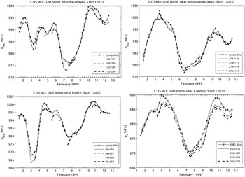
Figure 2 shows the time series of mean sea level pressure at stations Halley, Neumayer and Novolazarevskaya from SYNOP data and from COSMO Model runs, as well as the unreduced surface pressure at the Kohnen station from AWS data and COSMO Model runs. For each station the model data for the four nearest grid points are given. The plotted time series are the results from the first 24 hours of model runs starting at 12 UTC on each day from 1 to 11 February 1999; for 12 UTC the results are plotted from both successive runs. The sequences of low and high pressure episodes in the SYNOP data and the COSMO Model records agree well. Although observation data and model data differ at the starting time of the model run, the difference does not systematically increase with simulation time.
Time series of mean sea level pressure at Neumayer, Novolazarevskaya and Halley stations and of surface pressure at Kohnen station. Observed values are from SYNOP data and from AWS data, respectively. Simulated values are valid for the four COSMO Model grid points nearest to the stations. Results are plotted from successive model runs started at 12 UTC on 1–11 February 1999.

Simulated mean sea level pressure at the grid points surrounding each station are very close among themselves, as seen in Fig. 2 for Halley, Neumayer and Novolazarevskaya. For Kohnen the unreduced surface pressure is plotted. Two grid points have very similar height and pressure values, and the differences at the other two points are primarily due to differing surface heights. With these similarities in mind, we assume the data from the grid point closest to the station to be representative.
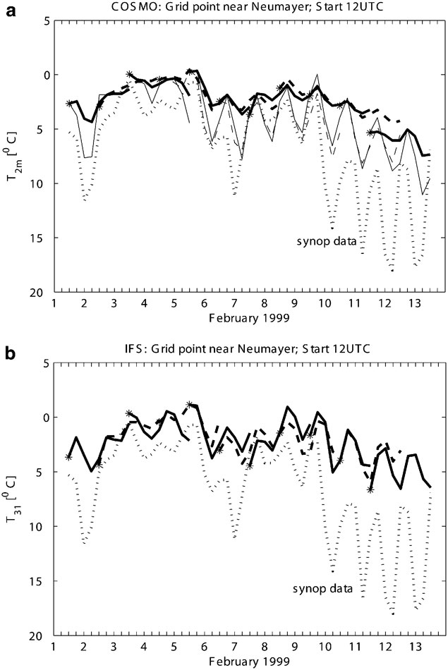
Another routinely observed parameter is the 2 m temperature. Figure 3a shows the time series for the simulated 2 m temperature and the SYNOP data for Neumayer. Since the model values are interpolated from the temperatures at the surface and at the lowest model layer (approximately 30 m above surface), the simulated 2 m temperature strongly reflects surface temperature. The results from the standard model run (thick lines) capture the general warming and cooling during the 12 days under consideration. However, the daily cycle is too weak, and a warm bias exists.
a. Time series of 2 m temperature at Neumayer station at grid point 170/199 for successive 48 hr simulation runs with overlapping periods. Thick lines = standard model run, thin lines = LFS run. Start of new run is marked by *; successive runs are alternately plotted in solid and dashed lines. b. As (a) but for temperature from the IFS model run at the lowest model level at grid point 164/39.
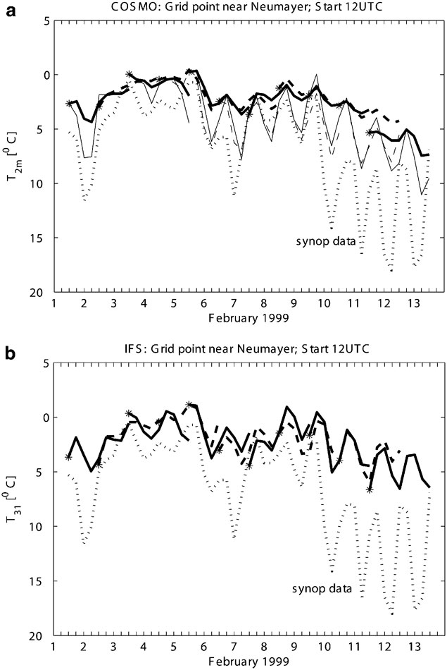
Initial 2 m temperatures differ strongly from the observed data. Initial and boundary values follow from vertical and horizontal interpolation of the IFS data given on a much coarser horizontal grid. The IFS temperature at the lowest model level (approximately 30 m above surface) is shown in Fig. 3b. Again, the modelled temperature is generally higher than the 2 m temperature in the SYNOP data, hence, the initial bias in the COSMO Model results is due to the information from the driving model. The initial surface and soil temperatures for the COSMO Model are taken from corresponding IFS data which were calculated using a parameterization which is very different from that used in the COSMO Model.
Hines et al. (Reference Hines, Bromwich and Liu1997a, Reference Hines, Bromwich and Cullather1997b) also observed a temperature bias in their simulations of the Antarctic atmosphere. They found an overestimation of downward longwave radiation due to excessive cloud condensate concentrations, and were able to improve the results by removing the cause of the latter. With regard to the COSMO Model simulations, however, cloud condensate concentrations are not excessive (see section below) when compared to the values shown by Hines et al. (Reference Hines, Bromwich and Cullather1997b, after their correction); furthermore, results from a model run in which radiation transfer is not affected by clouds are very similar to those given in Fig. 3a for the standard run. Thus the treatment of cloud condensate is not the primary origin of the bias of simulated near-surface temperature.
Another potential source of error in the near-surface temperature is the parameterization of heat conduction in the underlying snow and soil. Forcing the values of heat conductivity and density of snow to the low values of freshly fallen snow (LFS run; see Appendix) yields a stronger daily cycle in 2 m temperature, see thin lines in Fig. 3a, by reducing the temperature minima during night, while the daily maxima remain close to those in the standard run. This result suggests that in future the COSMO Model snow and soil treatment should be modified for Antarctic conditions. Nevertheless, the modification of the snow parameters alone cannot remove the general warm bias.
It appears that the deficiencies in the near-surface temperature as simulated in the standard run follow from a combination of the initial values from IFS, the treatment of heat transport within snow, and eventually also the treatment of radiation transfer and of sea ice. The assessment for the simulated 2 m temperature for the regions around the other three stations is similar to that discussed for Neumayer, except the lack of a general warm bias at Novolazarevskaya.
Vertical profiles
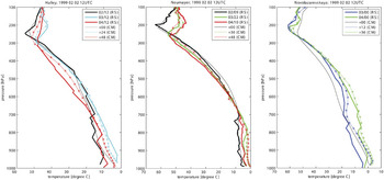
The evolution of the temperature profile during the simulation period started at 2 February 1999 12 UTC is shown in Fig. 4 for the grid points nearest to the stations Neumayer, Halley, and Novolazarevskaya, along with the radiosonde data. The timing of the Neumayer radiosondes does not match the model output timing. The profiles are plotted on pressure levels as output from the model and the data bank, respectively, to avoid interpolation onto standard pressure levels. The model data certainly cannot reproduce the vertically highly resolved profiles from the Neumayer radiosondes.
Vertical profiles of temperature from the COSMO Model runs (thin line = standard run, asterisks = LFS run) valid for grid points nearest to Halley, Neumayer and Novolazarevskaya, and from radiosonde data (thick lines). Time is given in hours after simulation start at 2 February 1999 12 UTC, and for the start of the radiosonde in day/hour (UTC), respectively.

Model and radiosonde data for the temperature profile agree with respect to the weak temperature decrease with height within the lower part of the troposphere and the stronger decrease in the upper part. Model data reproduce the observed warming during the first 24 hours and also, in case of the Halley data, the cooling during the last 24 hours of the period. Height and variation of height of the tropopause also agree.
A clear warm bias is seen in the simulated temperature within the lower troposphere. This is more pronounced close to the surface, and the bias is already present in the initial state. The situation is extreme at Halley with an initial difference of nearly 10 K. It is not yet clear whether this initial warm bias near the surface is responsible for the warm bias found later in the simulations throughout a thick layer, as discussed for the warm bias in the 2 m temperature at Neumayer. Temperature profiles as follow from the LFS run are also shown in the figure. Results from the two model runs are very close for this 2 February case. A slightly colder lowest model layer is found in the LFS run only in the Halley and Novolazarevskaya profiles. This small difference should be expected, as the simulated 2 m temperature only weakly distinguishes between the two model runs started at 2 February (Fig. 3a for Neumayer).
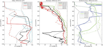
We use the relative humidity with respect to liquid water saturation as a measure for water vapour content. Unlike specific humidity, relative humidity does not generally decrease with height. In Fig. 5 the model results from the standard (thin line) and the LFS run (asterisks) are given along with the relative humidity at ice saturation (dashed lines) and the radiosonde observations (thick lines). Results are similar for the two model runs.
As Fig. 4 but for vertical profiles of relative humidity (with respect to liquid water saturation). Dashed line gives relative humidity at ice saturation for COSMO results (standard run).

The radiosonde data were not corrected after retrieval from the database. It should be noted that the stored dew points at Halley and Novolazarevskaya are equal to the observed temperature at sporadic levels (these are the levels with 100% relative humidity in Fig. 5) even aloft. At least for the Novolazarevskaya profiles, these data should be questioned, since water-saturated conditions are not expected at levels above 400 hPa and temperatures below -30°C. The simulated profiles show the development of very moist and of dry layers. Despite large deviations in the initial profile, the model reproduces the arrival of moist air in the middle troposphere, though the exact height and amount differ.
At Neumayer, the air is more or less water-saturated up to about 600 hPa after 24 and 48 hour simulation time. At 24 hours this is in agreement with the observed nearly saturated profile. At 48 hours observations show a slightly ice-subsaturated layer. Yet we should assume a temporarily higher moisture amount, since precipitation was reported for the period 6 to 12 UTC.
The COSMO Model tends to overestimate relative humidity. For regions prone to cloud formation, this may be related to the assumption in the cloud microphysics parameterization that the initiation of cloud ice requires water saturation at T ≥ -25°C, which supports the maintenance of (nearly) water-saturated layers. Indeed, we find at Neumayer and Halley nearly water-saturated conditions over a long period in the comparatively warm lower and mid-troposphere at T ≥ -25°C. An example of a mismatch between model result and observation is the distribution at Halley after 48 hours of simulation time, when the modelled relative humidity is far too low, apart from the near-surface layers.
In summary, differences between model results and observed data in surface pressure, temperature, and relative humidity in the earlier part of the simulation run seem to be due, at least partly, to model initialization. General warming and cooling as well as moistening and desiccation away from the surface are in most cases reasonably well reproduced, as seen in the evolution of the time series of surface pressure, temperature and relative humidity profiles and the passage of low and high pressure systems. Matters are less satisfying near the surface, where the model misrepresents the daily cycle in temperature, probably influenced by deficiencies in the snow treatment in the standard model version, and the simulated temperature profiles show a warm bias.
The synoptic situation
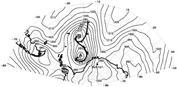
From 2 February 1999 weather in DML was influenced by synoptic depressions and related precipitation. The synoptic situation is similar to that which Noone et al. (Reference Noone, Turner and Mulvaney1999) describe as that most frequently bringing precipitation of more than 1 mm during a day in the Kohnen region. Two systems develop in a meridionally elongated trough east of Argentina, named A and B, respectively. Low A reaches the coast of Antarctica on 2 February 1999 (Fig. 6), and on satellite images the cloud band of the occluded front was seen to extend into DML. Now low A has its minimum central pressure of 955 hPa.
Mean sea level pressure in hPa for 2 February 1999 12 UTC from IFS operational analysis.

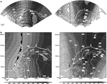
Figure 7 shows surface pressure (reduced to mean sea level) and near-surface wind fields, as well as geopotential and temperature fields at the 500 hPa level, valid at 3 February 12 UTC as simulated by the COSMO Model. Results from the IFS simulation, which provides the driving fields, are shown for comparison. By this time, Low A has travelled into the Southern Weddell Sea and will subsequently decay. The surface depression is found at the front side of the trough at 500 hPa with the geopotential wave slightly ahead of the temperature wave. The northerly flow on the eastern side of the trough brings warm maritime air far into DML. To the rear of the surface occlusion, polar air advances northward. Around this time, the minimum mean sea level pressure is registered at Halley and Neumayer (Fig. 2). At Halley, Neumayer and Novolazarevskaya the sequences of temperature profiles in Fig. 4 show a warming of the whole troposphere due to the advection of warm air. Advection of maritime air increases the relative humidity at Halley and Neumayer (Fig. 5). Later on, temperature and relative humidity sink at Halley due to the southerly flow of cold air.
24 hour simulation valid at 3 February 1999 12 UTC using a. global IFS model, b. COSMO Model. Left: mean sea level pressure (in hPa) and wind vectors at the lowest model layer (approximately 30 m above surface, see scaling for windspeed in m s-1) plotted at every 10th (COSMO results) and 5th grid point (IFS results), respectively. Right: Geopotential (in gpdm, isolines) and temperature (in °C, shaded) at p = 500 hPa. COSMO Model domain is marked in the figures for IFS results.

The overall synoptic patterns are similar in the COSMO and IFS model simulations. Marked differences in the mean sea level pressure fields are evident only in the south-eastern part of the plateau. This may be due to the reduction of surface pressure, because computed temperatures at the lowest model levels differ in this region.
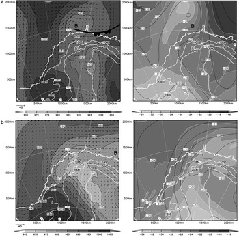
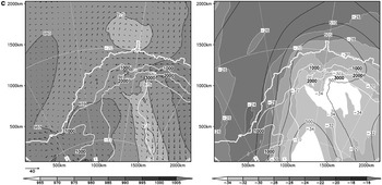
After 3 February, pressure and geopotential drop over a large area. The second low (B) reaches the northern coast of DML around 5 February 00 UTC with its occluded front parallel to the Antarctic slope (Fig. 8a). By this time the southward advance of warm air has stopped, and to the rear of Low B, polar air approaches from the west. Low B moves eastward along the coast and reaches the eastern boundary of the simulation area on 6 February around 06 UTC (Fig. 8b). At the same time, a new weak low pressure system develops at the western coast of DML in the offshore current, which then slowly travels eastward along the coast of DML. The overall drop of pressure and geopotential continues, and horizontal pressure gradients become weak (see Fig. 8c). The general pressure decrease is seen in the time series for all four stations in Fig. 2.
Left: COSMO Model results of mean sea level pressure (in hPa) and wind vectors at at lowest model layer (approximately 30 m above surface) plotted at every 10th grid point (see scaling for windspeed in m s-1). Right: Geopotential (in gpdm, isolines) and temperature (in °C, shaded) at p = 500 hPa. a. 12 hour simulation valid at 5 February 1999 00 UTC, b. 6 hour simulation valid at 6 February 1999 18 UTC, c. 12 hour simulation valid at 8 February 1999 00 UTC. Data from a boundary region of 10 grid points are excluded.


Gradients in pressure, temperature and geopotential fields are found in the COSMO-simulations at the outflow boundary, that is at the southern and eastern edges of the model domain, see Fig. 7. These are boundary effects which arise when travelling synoptic patterns as simulated by the COSMO Model are confronted with the prescribed boundary conditions set by the driving IFS model. Therefore, a boundary region of 10 grid points is discarded as buffer zone in the fields presented in Fig. 8.
Total condensate amount
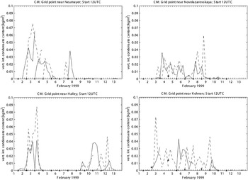
Cloud condensate is crucial for precipitation formation and also for radiation transfer. In this section the vertically integrated cloud water and ice content is examined with regard to its time series at selected grid points and to its horizontal distribution. Since no observation data are available for verification, we can only evaluate whether the order of magnitude is reasonable, whether there is a systematic trend during the 48 hour simulation runs, and whether the results for maritime and continental areas differ.
The time series of vertically integrated total cloud condensate content is given in Fig. 9 for the gridpoints nearest the four stations for the successive 48 hour simulation runs, with new runs started at 12 UTC on each day. The maximum value is nearly 0.09 kg m-2 or mm w.e. depth (Halley, valid at 3 February 1999 18 UTC after 30 hour simulation time). This is lower than the zonally averaged mean values of some 0.2 to 0.5 mm w.e. depth reported by Hines et al. (Reference Hines, Bromwich and Cullather1997b; Fig. 3) for June 1988, yet, the authors regard those values as too high.
Time series of vertically integrated cloud water and cloud ice content at Neumayer, Novolazarevskaya, Halley and Kohnen. Model data are valid at the grid point nearest to each station. Results are plotted from successive model runs started at 12 UTC on 1 to 11 February 1999. Start of new run is marked by *. Successive runs are plotted in different line styles.

The successive time series shown in Fig. 9 start with a condensate-free air column except at Kohnen. Within the following few hours (the spin-up time) clouds are formed and intensified. Later on, no systematic increase of condensate amount is found with increasing simulation time.
Stone (Reference Stone1993) presents partial densities of cloud ice for wintertime clouds at the South Pole with base temperatures below -30°C. These estimated concentration values are somewhat lower than those seen in the vertical profiles simulated by the COSMO Model for the four stations. The differences may in part be attributed to the differing temperatures.
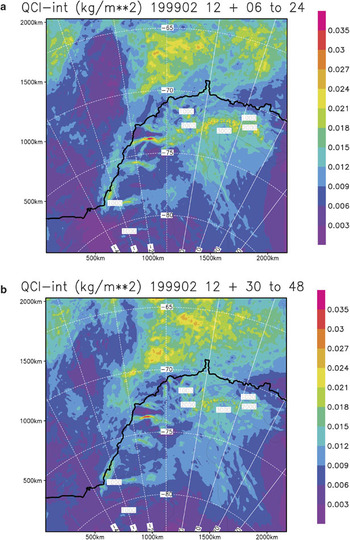
The horizontal distribution of the time average of vertically integrated total cloud condensate is shown in Fig. 10 for the period 2 February 18 UTC to 12 February 12 UTC. The average values are calculated from the time series composed of a) the interval of 6–24 hour and b) the interval of 30–48 hour simulation time of the model runs. The first 6 hours of simulation time are excluded to avoid effects of spin-up. Both distributions of total condensate amount show the same gross features, namely i) a region of high values over the ocean north of 70°S and east of 20°W in maritime air, ii) a cloud zone over the continent with monotonically decreasing intensity toward the interior, iii) pronounced maxima on the windward side along the steep margins of the plateau, in which extreme values within a small region near 15°W/74°S seem to be excessive, and iv) a dry zone over the ocean west of 20°W, which was not affected by the fronts. Fig. 10a & b differ, however, in details such as the spatial structure of the region referred to under (i). Thus, different precipitation patterns can also be expected.
Horizontal distribution of average vertically integrated cloud water and cloud ice content in kg m-2, valid for the period 2 February 1999 18 UTC to 12 February 1999 12 UTC. Time series are composed of a. the interval of 6–24 hour, b. the interval of 30–48 hour simulation time of the model runs. Boundary region of 10 grid points not shown.

Boundary effects are found in the fields of total cloud condensate amount within 100 km of the domain edge (not seen in Fig. 10, because the boundary region is not plotted). Distributions of condensate amount in the boundary region deviate not only due to the different simulation times, but also due to the different prescribed boundary conditions following from successive IFS runs.
The amount of cloud condensate strongly depends on the assumptions underlying the parameterization, including the nucleation conditions for ice particles and the autoconversion threshold values. Excessive cloud condensate concentrations are prevented by setting threshold values in the cloud microphysics parameterization of the COSMO Model equal to zero. The contributions of cloud liquid water and cloud ice are steered by the prescribed number of nucleated ice crystals and by the moisture threshold for ice nucleation. When the number of nucleated ice crystals is reduced compared to the standard value used in the COSMO Model, the amount of cloud ice decreases, while cloud water is present more frequently. The choice of such steering parameters may be optimized in future research, provided information about the condensate concentrations and distributions are available for the Antarctic atmosphere.
Simulated precipitation
Time series
The good agreement between simulated and observed pressure changes due to passing depressions (Fig. 2) implies that we can examine the timing and amount of precipitation. Time series of precipitation are discussed for the four grid points near Halley, Kohnen, Neumayer and Novolazarevskaya, and are compared to observation data. A spin-up effect in precipitation is to be expected due to the spin-up effect in cloud condensate concentration.
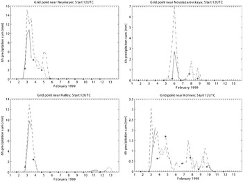
Time series of 6 hour precipitation sums (allocated to the end of the period) are given in Fig. 11 for all eleven 48 hour simulation runs such that the time series from successive simulations overlap. Precipitation rates are given in mm water equivalent (w.e.). Precipitation at the four grid points closest to each of the four stations have similar evolution, although peak values may differ. Therefore, we discuss here only results from the grid points closest to each of the stations (Fig. 11), while the horizontal precipitation distribution will be discussed later.
Time series of simulated 6 hour precipitation sums (in mm w.e.; allocated to the final time of the period) at Neumayer, Novolazarevskaya, Halley and Kohnen. Model data are valid at the grid point nearest to each station. Results are plotted for the 48 hour simulation period from successive model runs started at 12 UTC on 1–11 February 1999. Start of new run is marked by *. Successive runs are plotted in different line styles.

The strongest precipitation signal near Halley, Neumayer and Kohnen occurs around 3 February and is related to the Weddell Sea cyclone A (Fig. 7). A second precipitation event is reflected in the time series for Neumayer, Kohnen and Novolazarevskaya for 4–6 February, when the low pressure system B moves along the coast (Fig. 8a). For the Kohnen grid point, precipitation is also simulated for the days after 6 February at a rate of the order of magnitude of 1mm per 6 hours. This long lasting precipitation event is also found in the overlapping periods of successive simulation runs. Similar to the time series of condensate content (Fig. 9), no systematic trend is found in the precipitation sums for any of the grid points within the 48 hour simulation time of each run.
Successive model runs show only moderate agreement in the precipitation sums within the overlapping periods (Fig. 11). This is at least partly due to the fact that the precipitation sums from the first 6 hours of the runs are mostly lower than later sums, which illustrates the spin-up effect; there are only few exceptions, such as at Neumayer in the run started on 3 February and at Kohnen in the run started on 4 February. Because we wish to examine composite time series of precipitation for the 12 day period, care must be taken in selecting the periods from each of the model runs. We must compromise among avoiding accumulated model errors and excluding spin-up effects.
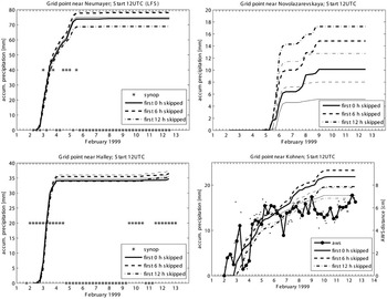
Composite time series of accumulated precipitation in which the first 0, 6, and 12 hours, respectively, are disregarded, are shown in Fig. 12 for grid points close to each of the stations in both the standard and LFS runs. All three time series are valid for 2 February 00 UTC to 12 February 12 UTC. The series agree with regard to the timing of the precipitation event, but differ in magnitude.
Composite time series, valid from 2 February 1999 00 UTC to 12 February 1999 12 UTC, of accumulated precipitation at Neumayer, Novolazarevskaya, Halley and Kohnen. Model results are for the COSMO Model grid points nearest to each station. Thick lines give results from the standard run, thin lines from the LFS run. From each model run the first 0, 6 and 12 hours are discarded. Asterisks mark reported snowfall in SYNOP data at Neumayer and Halley during the previous 6 hours. For Kohnen, AWS distance (i.e. height distance between AWS sensor and surface relative to the value at 2 February 1999 00 UTC, with opposite sign) is given for every 2 hours (small dots) and 6 hours (thick line with dots) according to the r.h.s. scale.

We start with discussion of results from the standard run. Accumulated precipitation at three of the four grid points (Fig. 12) is largest when the first 6 hours of simulation time are disregarded. The only exception is for Novolazarevskaya: The strong precipitation event from 5–6 February with a pronounced peak rate of 7 mm per 6 hours during the period from 30 to 36 hours, is captured only if the results from later simulation times are included. On the other hand, the lowest accumulated precipitation is only found in two out of four cases, when the first 24 hours of simulation time are considered.
The problem of model spin-up and the question as to which forecast period is used for precipitation time series were discussed by Turner et al. (Reference Turner, Connolley, Leonhard, Marshall and Vaughan1999) in their preparation of a precipitation climatology for Antarctica from ECMWF re-analysis data. Examining the 15 year period 1979–1993, they found that 12 hour precipitation sums are about 9% higher during the second 12 hour periods than during the first. As seen from Fig. 11 for the 11 day period, the deviations in precipitation sums for different time intervals of the model runs also show the opposite effect on some days. Thus, the deviations for particular weather events may be larger than deviations averaged over several days, or even years over a large region.
Assessment of simulated precipitation is problematic due to well known difficulties in measuring precipitation rates in polar regions. For the present study, SYNOP information about precipitation type is available at Halley and Neumayer at 3 hour intervals. If no precipitation was reported for the previous 6 hours, this is marked in Fig. 12 by an asterisk located at zero; otherwise the asterisk is placed at a non-zero value for accumulated precipitation without further specification. Drifting or blowing snow reports are disregarded. The periods during which the strongest precipitation events are simulated for Halley and Neumayer agree with observational evidence. This is true regardless of the length of the discarded initial period. The COSMO Model results show light precipitation near Halley for the latest days of the simulation period, which agrees with the SYNOP reports.
At Kohnen, the height of the AWS sensor above the surface was recorded every five minutes and stored as two-hourly averages (Kohnen AWS data provided by IMAU, University Utrecht). This distance is modified by precipitation, snowdrift, sublimation, compaction, and related processes, and it is impossible to unambiguously attribute a registered distance change within a day or even shorter time interval to a particular process. Therefore, one can relate distance decrease uniquely with precipitation only in very few events, as discussed by Reijmer & Van Den Broeke (Reference Reijmer and Van Den Broeke2001). From a yearly time series of changes of the distance of the AWS sensor, these authors identified four major precipitation events in qualitative agreement with ECMWF model forecasts.
Distance between the AWS sensor and the surface relative to the distance at 2 February 00 UTC is given every 2 hours (small dots) and 6 hours (thick line with dots) in Fig. 12. This property is plotted with opposite sign, such that the line ascends for decreasing distance to suggest accumulation of snow, and is hereafter referred to as ‘AWS distance’. Change in the AWS distance is not converted into a precipitation rate, because the density of the freshly accumulated snow is unknown. Large variations in AWS distance values in both directions mean, that one cannot associate even jumps in the 6 hourly time series to individual precipitation events. However, an overall change of AWS distance of about 7 cm is clearly discernible. Although no information is available regarding snowdrift, compaction, and sublimation, this strong height change is taken to indicate the occurrence of significant precipitation during this period. A 7 cm surface height change is equivalent to 10.5 to 23.5 mm w.e. if the density of snow is assumed to be between 150 kg m-3, typical for freshly fallen snow (Garratt Reference Garratt1992), and 335 kg m-3, typical for long term accumulated snow at Kohnen (Reijmer & Van Den Broeke Reference Reijmer and Van Den Broeke2001). In this context, the simulated precipitation amount of some 20 mm w.e. is large, yet reasonable.
The model simulates more or less continuous precipitation at Kohnen throughout the period (Figs 11 & 12). This is the only station of the four where clouds are already present in the initial field, as is the case in a limited region around Kohnen. The AWS data show an overall snow height increase primarily until 5 February, probably due to precipitation. Later, the average level remains nearly constant with superimposed fluctuations. It is speculated that some snowfall followed by consolidation may contribute to the fluctuations, although the actual origin cannot be stated for certain.
Simulated precipitation sums at Kohnen may be compared with annual accumulation from other sources. Oerter et al. (Reference Oerter, Wilhelms, Jung-Rothenhäuser, Göktas, Miller, Graf and Sommer2000) estimate 62 mm w.e. as the climatological mean value over the past 200 years, and Van Den Broeke et al. (Reference Van Den Broeke, Reijmer and Van De Wal2004) estimate a mean of 79 mm w.e. from AWS data from 1998 to 2001. If we assume the annual precipitation sum to be roughly equal to the annual accumulation, then the simulated 20 mm w.e. for the 10 day period is indeed a large portion of total annual accumulation, although not unrealistic. Compared with daily precipitation sums from AMPS simulations for the years 2003, 2004 and 2005 (http://polarmet.mps.ohio-state.edu/PolarMet/ampsdb.html on a horizontal mesh grid of 30 km) the COSMO Model results are mostly of similar magnitude. Bearing in mind that simulated precipitation sums increase with increasing resolution (Mass et al. Reference Mass, Ovens, Westrick and Colle2002), the COSMO Model results are high, but not unreasonably for a particularly strong precipitation event.
The LFS and standard runs show the same spin-up behaviour for accumulated precipitation. Time series for the standard and LFS runs at the Neumayer and Halley grid are nearly identical with the latter resulting in slightly more precipitation. On the other hand, the precipitation sums for Novolazarevskaya and Kohnen are considerably lower in the LFS run, indicating a sensitivity to the treatment of heat conduction in snow. The timing of precipitation is the same in both model run series, except that the last precipitation event at Novolazarevskaya around 9 February 1999 00 UTC in the standard run, is missing in the LFS run.
Horizontal distribution
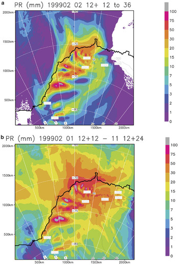
The horizontal distribution of accumulated precipitation during the 24 hour period from 3 February 1999 00 UTC to 4 February 1999 00 UTC and for the full period of 10.5 days from the standard run is shown in Fig. 13. Those 24 hours are characterized by strong precipitation, hence the period strongly influences the sum over a longer period. Precipitation occurs within most of the domain, and the region with more than 10 mm w.e. reaches far inland on DML. Large precipitation sums near the coast and at the margin of the DML plateau dominate the field. The 24 hour precipitation sums (Fig. 13a) show short, 50 to 100 km, wavelength variability near the coast, and two pronounced low precipitation zones in the western part of the plateau, followed in south-east direction by a SW–NE oriented precipitation band. The distribution for the whole 10.5 day period (Fig. 13b) is slightly smoother, and more precipitation is found over the ocean, while the short wavelength variability near the west coast remains clearly visible. A different horizontal structure is found on the plateau, that are precipitation bands with NW–SE orientation. All these spatial structures have a width of 50 km or more and thus can be considered well resolved by the model run at 7 km mesh width, but are at the limit of resolution when mesh sizes of 20 km and more are used.
a. Horizontal distribution of simulated precipitation sums (in mm w.e.) valid from 3 February 1999 00 UTC to 4 February 1999 00 UTC from a COSMO Model run started at 2 February 1999 12 UTC. Boundary region of 10 grid points not shown. b. As (a), but valid from 2 February 1999 00 UTC to 12 February 1999 12 UTC. Model runs are started each day at 12 UTC, and the first 12 hours of simulation time are skipped as spin-up time.

Localized precipitation maxima exceeding 100 mm occur along the steep terrain on the west and north-west side of the continent. These are the windward slopes during the warm and moist flow regime (Fig. 7b). Unfortunately, no observational evidence is available for validation of this result. Large precipitation sums due to strong forcing by terrain are frequently reported for high-resolution modelling, for example Gravert et al. (Reference Gravert, Colle and Mass2005) and Mass et al. (Reference Mass, Ovens, Westrick and Colle2002), who considered those sums to be overestimates. Furthermore, Monaghan et al. (Reference Monaghan, Bromwich, Powers and Manning2005) found precipitation sums exceeding 500 mm during the three summer as well as autumn months on the windward side of Ross Island in the detailed maps of precipitation distribution for the McMurdo region as simulated by AMPS with a grid size of 3.3 km. The maxima were due to a favourable combination of orography and cyclone tracks. The high precipitation sums on the windward slopes in the present simulations (Fig. 13) are thus reasonable with regard to the occurrence of local heavy precipitation due to orographic forcing, although exaggerated in magnitude.
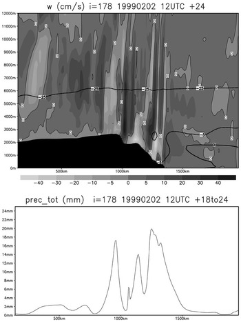
Because the fronts do not penetrate far inland, precipitation sums decrease toward the south and south-east in DML. The monotonous decrease seen in the large scale climatological distribution given by Bromwich (Reference Bromwich1988) is not produced by our high-resolution simulations and even on the plateau, adjacent regions of high and low precipitation appear in the pattern of 10 day precipitation sums. On the western side of the continent, a flow with a northerly component (Fig. 7b) crosses mountain ridges, and topographic effects may be responsible for the small scale pattern of high precipitation on the upwind side and low precipitation on the downwind side. It may be that gravity waves excited by topography trigger the formation of precipitation on the plateau in our simulations. As an example, in Fig. 7b the near-surface flow is nearly perpendicular to the northern coast of DML and carries moist air. A vertical cross section in the south–north direction of 1239 km from the western model boundary is shown in Fig. 14 for vertical velocity w. While vertical motions are weak above the ocean, intense up- and downwind cells are seen above the slope and above the plateau. The strong near-surface downwind cells are connected with the deflection of the flow by the obstacle in the downslope direction towards the west. The lower part of Fig. 14 gives 6 hour precipitation sums. A sequence of pronounced precipitation maxima is found toward the south, followed far inland by additional, much weaker, peaks. The peaks are on the downstream side of the upwind cells. The w-field is in some respects similar to the fields known from idealized gravity wave studies (e.g. Smith Reference Smith1979). Differences may be attributed, at least partly, to deviations in the topography from that adopted in the idealized studies, and certainly also to the particular weather situation. Further investigations should clarify the influence of gravity waves excited by topography and their influence on mesoscale variations in precipitation over Antarctica.
Vertical cross section of vertical velocity (in cm s-1, upper figure) together with 0°C, -5°C, -25°C isotherms and 6 hour precipitation sum (in mm, lower figure) in the south–north direction along a line 1239 km from the western model boundary from the simulation started at 2 February 1999 12 UTC, valid at 3 February 1999 12 UTC.

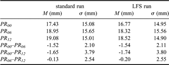
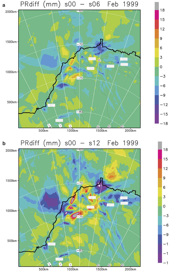
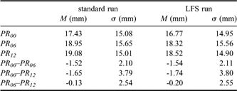
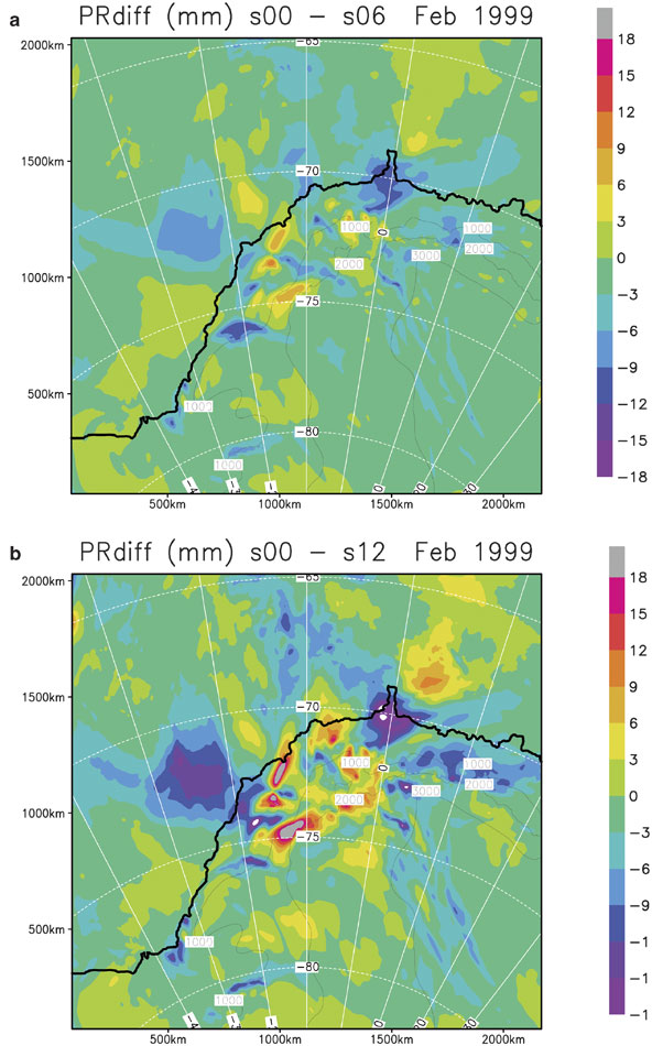
The general precipitation distribution produced in our simulations is independent of the spin-up effect. The horizontally averaged precipitation sums are given in Table I for discarded initial periods of various lengths. Differences in accumulated precipitation are roughly 10%. The standard deviations of the difference, however, are larger than the mean difference. These results hold for the standard as well as the LFS runs. The large variation becomes obvious in the horizontal distributions of the differences in precipitation when discarding initial periods of the model runs of various lengths (Fig. 15). The distributions appear patchy, and positive as well as negative differences are found. Among other factors, small phase shifts in the location of the synoptic systems or differences in the intensities of the depression between the results from successive model runs will contribute to the high spatial variability of precipitation.
Horizontal mean value M and standard deviation σ of simulated precipitation sums valid for 2 February 1999 00 UTC to 12 February 1999 12 UTC for the standard and for the LFS run. PRn denotes the precipitation sum from a composite time series, when the first n hours of the simulation time are excluded. Statistical values are taken for the whole model domain except a boundary region of 10 grid points.
a. As Fig. 13b but for the difference between precipitation sums with 0 hours and with 6 hours spin-up time. b. As (a) but for 0 hours and 12 hours spin-up time.
Summary and discussion
Precipitation is an important parameter in the mass balance of the Antarctic ice sheet. An episode in which frontal cloud systems brought precipitation far inland to Dronning Maud Land (DML) is investigated by numerical simulations to gain insight into the spatial distribution and temporal evolution of precipitation. The simulations are performed with the high-resolution COSMO weather forecast model.
Model results are compared with observational data from four Antarctic stations (Halley, Neumayer, and Novolazarevskaya at the coast, Kohnen on the plateau of DML) to assess the quality of the simulations. The development of surface pressure is well reproduced by the model, and the simulated vertical profiles of temperature and relative humidity mimic the gross features of the observed profiles. However, the model produces a distinct warm bias in the lower troposphere, and the 2 m temperature lacks a pronounced daily cycle. The warm bias is present in the initial fields used for model initialization and thus carries forward in model results. The weak daily cycle appears to be caused to some extent by the treatment of processes in snow and soil in the standard model configuration. Shortcomings in the model temperature fields may also be related to the treatment of radiation transfer and sea ice, but are likely not due to the present treatment of clouds. Unfortunately, the sparsity of observational data limits a detailed evaluation of the model results.
Precipitation is more difficult to assess, because information is available only from two stations on the occurrence of snowfall. Additional observations from an automatic weather station monitoring the distance between the sensor and the snow surface are available, but the signals due to snowfall, drifting snow, and sublimation cannot be separated. The evaluation of modelled precipitation rate is further complicated by the fact that model data represents the mean precipitation over a grid cell, while observational data provides point measurements.
The limited comparison we are able to make indicates the model’s performance to reproduce the overall weather evolution including thermal and hygric conditions. The timing of simulated precipitation agrees well with snowfall observations at the four stations. The amount of modelled precipitation is large compared to accumulation climatology and to AMPS simulations, but is not unrealistic for a particularly strong precipitation event. However, precipitation sums greater than 100 mm within 24 hours in some regions with steep topography are considered excessive even in the absence of observations. The local precipitation sums are sensitive to the treatment of processes in the ground (Fig. 12), although in the spatial and temporal average the statistics of the sums are only weakly affected (Table I).
Precipitation time series at the three locations close to the coast are dominated by short episodes. On the plateau near Kohnen, snow is simulated more or less continuously throughout most of the period under consideration.
The spatial distribution of modelled precipitation is dominated by the topographic effect, in particular, due to the steep margin of the plateau. A decrease in precipitation is found toward the interior, but this decrease follows neither increasing distance from the coast nor the topographic contours. Far from the coast precipitation exceeds 20 mm w.e. within the 10.5 day period over a large region, extending far inland in form of tongues. Deviations from the climatological precipitation distribution as given by Bromwich (Reference Bromwich1988) are caused by the path of the frontal cloud systems.
The time series of 6 hour precipitation sums (Figs 11 & 12) as well as the precipitation amount during the whole episode (Fig. 13a & Table I) depend on the length of the initial time span excluded from the interpretation as spin-up time. On the whole, precipitation amount increases with increasing length of the excluded spin-up time; locally, however, matters may be different. This holds for the standard and the LFS runs and is not a particular feature of results from the COSMO Model used in this study. Turner et al. (Reference Turner, Connolley, Leonhard, Marshall and Vaughan1999) found in ECMWF re-analysis data an increase in a 15 year mean precipitation of about 10% if the first 12 hours of each simulation were disregarded. Our findings suggest roughly the same difference for area-averaged precipitation sums. On small space and time scales, however, the deviations may be much larger and of positive as well as negative sign.
It remains unclear whether the strong spin-up effect on precipitation can be reduced by using other data sets than the IFS data to drive the limited area model. Despite this and other uncertainties, the case study presented here shows that the COSMO Model can reproduce to a sufficient degree of accuracy weather evolution including precipitation at high spatial and temporal resolution in high latitudes. In addition, precipitation falling during particular weather events is much more variable in space than expected from existing climatologies.
Acknowledgements
The authors thank the anonymous reviewers for their comprehensive and helpful work and C. Hulbe (Portland State University) for useful suggestions. We acknowledge the support of R. Brauner (DWD, Hamburg) in the interpretation of the synoptic situation. Kohnen AWS data were provided by IMAU, Utrecht, and the authors are thankful to C. Reijmer and M. van den Broeke. Initial and boundary data were provided by DWD and ECMWF. Thanks are also to the staff of DWD’s Business Area ‘Research and Development’ for substantial assistance. We particularly thank our colleagues J. Schwarz and H. Hellmer (Alfred Wegener Institute), who helped us with the language of this paper. The research was supported by priority program SPP 1158 sponsored by the Deutsche Forschungsgemeinschaft under grants WA1334/4 and BI816/1.
Appendix
The soil model
The soil model, named TERRA, predicts temperature and specific humidity at the ground. For an underlying ocean, sea surface temperature is kept constant during the integration time. Eight soil types are considered, out of which only land ice is of interest in this study. For this type, ice-saturation is prescribed at the surface, and in contrast to the treatment of other soil types, no further hydrological processes in the ground are considered.
The thermal part of TERRA uses a model with two soil layers and a snow layer to predict the temperatures at layer interfaces. As the lower boundary condition at the interface between the second soil layer and the lower deep soil layer, the temperature is assumed to be the climatological temperature, which is held constant during the integration run. Between the layer interfaces, a linear temperature profile is prescribed.
Heat fluxes between the various layers, the sensible and latent heat fluxes from the atmosphere, the budget of radiation fluxes at the surface and the heat flux due to melting and freezing are used to predict the mean temperatures of the layers. The resulting set of temperature equations is solved using the extended force-restore method (Jacobsen & Heise Reference Jacobsen and Heise1982). The initial conditions for the soil relevant temperatures are derived by horizontal and vertical interpolation of the IFS data.
The following parameters are used for land ice in the standard version of the model: Thermal conductivity λ = 2.26 kg m s-3 K-1, volumetric heat capacity ρc = 1.92 x 10⁻⁶ kg m-1 s-2 K-1, albedo α = 0.7. The thicknesses of the two soil layers are calculated to be Δz = 12.4 cm and 65 cm, respectively. For snow, thermal conductivity and density vary with water equivalent height between λsnow = 0.2–1.5 kg m s-3 K-1 and ρsnow = 500–800 kg m-3, respectively. An additional model run is performed with constant values for λsnow and ρsnow typical for fresh snow, λsnow = 0.1 kg m s-3 K-1, ρsnow = 150 kg m-3 according to Garratt (Reference Garratt1992); this model run is called the ‘constant–λ–fresh–snow run’ (LFS run).
The sea surface temperature (SST) is diagnosed from the field of the driving model, and sea ice is interpreted whenever SST < -1.7°C. SST is assumed constant during the model run.