


1 Introduction
Liners are widely used to mitigate noise emissions from ducts. In most of the practical applications, from air conditioning systems to aero-engines, a flow is present in the duct. The interaction between flow and sound in the vicinity of a lined wall is complex and, therefore, a precise description of the flow–acoustic coupling near a liner still attracts a lot of attention (Zhang & Bodony Reference Zhang and Bodony2012, Reference Zhang and Bodony2016; Tam et al. Reference Tam, Pastouchenko, Jones and Watson2014; Khamis & Brambley Reference Khamis and Brambley2016, Reference Khamis and Brambley2017). Surprisingly, under certain circumstances, instead of being attenuated, the sound can be amplified by a liner with a grazing flow. Indeed, it was observed that the transmission coefficient of a plane wave propagating through a liner in the flow direction can have a peak in amplitude larger than unity near the resonance frequency of the liner (Brandes & Ronneberger Reference Brandes and Ronneberger1995; Ronneberger & Jüschke Reference Ronneberger, Jüschke, Kurz, Parlitz and Kaatze2007; Aurégan & Leroux Reference Aurégan and Leroux2008). Such a sound amplification appears at high flow velocities when the liner has a low resistance. The fluctuating fields, the convection velocity and the growth rate of these unstable surface modes have been measured with optical technics (Marx et al. Reference Marx, Aurégan, Bailliet and Valière2010). Those measurements have shown that the unstable disturbance near the lined wall increases exponentially along the liner with a relatively low amplification rate. Since no saturation mechanism appears experimentally, a linear approach to this problem seems possible. It can also be noted that such convectively unstable modes may also exist above porous materials (Aurégan & Singh Reference Aurégan and Singh2014; Alomar & Aurégan Reference Alomar and Aurégan2017). In this case, the behaviour of unstable disturbances is more complex due to a slight flow inside the porous material which leads to separation on the downstream end of the material.
Many theoretical works have been performed on sound propagation in a lined duct with flow (Tester Reference Tester1973; Koch & Mohring Reference Koch and Mohring1983; Rienstra Reference Rienstra2003; Brambley & Peake Reference Brambley and Peake2006). A uniform mean flow was often assumed. To account for the effect of the infinitely thin vortex sheet on liner surface, the Ingard–Myers impedance boundary condition, which requires the continuity of particle displacement across the vorticity sheet, is enforced (Ingard Reference Ingard1959; Myers Reference Myers1980). With a uniform flow assumption plus the Ingard–Myers condition, a convective unstable mode (Tester Reference Tester1973) and a surface unstable mode (Rienstra Reference Rienstra2003) have been detected. However, some problems linked to the Ingard–Myers condition have been revealed: for instance, it is ill posed in the time domain (Brambley Reference Brambley2009), and it can over-predict sound attenuation by over 10 dB compared to the results from the linearized Euler equations (Gabard Reference Gabard2013). To overcome the problem of ill posedness, profiles with small but finite-thickness boundary layers were taken into account in the impedance boundary conditions (Brambley Reference Brambley2011; Rienstra & Darau Reference Rienstra and Darau2011; Khamis & Brambley Reference Khamis and Brambley2016). These models are able to predict an absolutely or convectively unstable mode over the lined wall. In the modelling of the flow–acoustic coupling near the lined wall, the importance of taking into account viscosity was demonstrated (Aurégan, Starobinski & Pagneux Reference Aurégan, Starobinski and Pagneux2001; Marx & Aurégan Reference Marx and Aurégan2013; Khamis & Brambley Reference Khamis and Brambley2017). Including turbulent viscosity leads to more accurate predictions of the growth rate and the velocity shape of the unstable surface mode above a liner. Also, the instability over the liner is influenced by the spatial development of the mean flow along the lined duct (Marx et al. Reference Marx, Aurégan, Bailliet and Valière2010; Xin et al. Reference Xin, Sun, Jing and Sun2016). All these efforts, however, are based on the assumption of a homogeneous impedance of the liner whereas in practice, this liner is constituted by a large number of small holes.
The limitations of the continuous impedance model in describing liners with flow have been revealed recently. It was first observed in experiments that two different impedances were measured according to whether the wave was propagating in the direction of flow or whether it was propagating against the flow (Renou & Aurégan Reference Renou and Aurégan2011). Since a uniform flow was assumed, the Ingard–Myers boundary condition was used in the impedance eduction from the experimental data. It could therefore be argued that the difference between these two impedances could be due to the imprecision of the impedance boundary condition. However, even taking into account the actual shear flow profile, the difference between the two impedances cannot be eliminated (Dai & Aurégan Reference Dai and Aurégan2016). The fact that liner impedance depends on flow direction has been verified in many laboratories, using different eduction methods and impedance boundary conditions (Spillere, Cordioli & Bodén Reference Spillere, Cordioli and Bodén2017), and even using the linearized Navier–Stokes equations for wave propagation (Weng et al. Reference Weng, Schulz, Ronneberger, Enghardt and Bake2018). From these experimental and theoretical works, we can draw the conclusion that the complex flow–acoustic coupling over the liner cannot be fully described by the currently used boundary conditions that involve a single quantity: an equivalent liner impedance.
The first objective of the present paper is, therefore, to examine the validity of the homogenized approach in describing the instability above a liner. To this end, a discrete approach of the aeroacoustic instability over a liner is developed. As sketched in figure 1, deep narrow cavities are periodically located along a duct containing a mean shear flow (period
 $W=L+S$
). The spacing between the adjacent cavities
 $S$
is small compared to the size
 $L$
of the cavity and very small compared to the acoustical wavelength. This liner can be seen as a two-dimensional (2-D) version of the ones used in the previous experiments (Aurégan & Leroux Reference Aurégan and Leroux2008; Marx et al.
Reference Marx, Aurégan, Bailliet and Valière2010). The acoustic and hydrodynamic disturbances are described by the linearized Euler equations (LEEs). To be able to describe the instability that appears in the experiments, some damping is required in the system. This is done artificially by adding a resistive layer at the inlet of the cavities and by adding an artificial damping to the hydrodynamic modes. This rough description of the viscous and turbulent effects only provides a qualitative comparison with the experiments, but it allows a better understanding of the mechanisms involved. For such a periodic system, the wave propagation can be calculated using the Floquet–Bloch theorem, which states that the field can be split into a 2-D periodic field modulated by a wave part of wavenumber
 $k_{B}$
. The Bloch wave and the scattering matrix of the system can be used to study the instability over the liner due to flow–acoustic coupling. Section 2 explains the multimodal method used to compute the scattering in one-cell and multi-cell liners and the calculation of the Bloch waves is described. Using this model, the results of the periodic approach are presented and analysed in § 3.1. It is first demonstrated that the aeroacoustic instability in the duct results from the coupling of a hydrodynamic mode in the boundary layer with the acoustic resonance of the cavities. Such an aeroacoustic instability can occur even if all transverse modes of the duct–cavity system are stable. It is also demonstrated that for the unstable behaviour of the configuration shown in figure 1, a homogenized method based on an equivalent wall impedance is a reasonable approximation to the complete Bloch analysis. In § 3.2, a case where each periodic cell consists of two cavities of different depths is considered. It is found that a small depth difference can suppress the unstable behaviour above the liner, and explanations from both the Bloch and the homogenized point of view are given.
(a) Sketch of flow–acoustic coupling over a liner, (b) a periodic unit of the discrete model.

2 Numerical model
2.1 Modal scattering in one cell
In an inviscid perfect fluid when the nonlinear effects are neglected, the propagation of small disturbances about a steady mean flow can be described by the linearized Euler equations (LEEs):
 $$\begin{eqnarray}\displaystyle & \displaystyle \left(\frac{\unicode[STIX]{x2202}}{\unicode[STIX]{x2202}t}+M_{0}f\frac{\unicode[STIX]{x2202}}{\unicode[STIX]{x2202}x}\right)u+M_{0}\frac{\text{d}f}{\text{d}y}v=-\frac{\unicode[STIX]{x2202}p}{\unicode[STIX]{x2202}x}, & \displaystyle\end{eqnarray}$$
 $$\begin{eqnarray}\displaystyle & \displaystyle \left(\frac{\unicode[STIX]{x2202}}{\unicode[STIX]{x2202}t}+M_{0}f\frac{\unicode[STIX]{x2202}}{\unicode[STIX]{x2202}x}\right)v=-\frac{\unicode[STIX]{x2202}p}{\unicode[STIX]{x2202}y}, & \displaystyle\end{eqnarray}$$
 $$\begin{eqnarray}\displaystyle & \displaystyle \left(\frac{\unicode[STIX]{x2202}}{\unicode[STIX]{x2202}t}+M_{0}f\frac{\unicode[STIX]{x2202}}{\unicode[STIX]{x2202}x}\right)p=-\left(\frac{\unicode[STIX]{x2202}u}{\unicode[STIX]{x2202}x}+\frac{\unicode[STIX]{x2202}v}{\unicode[STIX]{x2202}y}\right), & \displaystyle\end{eqnarray}$$
where all the quantities have been put in dimensionless form using:
 $$\begin{eqnarray}\left.\begin{array}{@{}c@{}}p={\displaystyle \frac{p^{\ast }}{\unicode[STIX]{x1D70C}_{0}^{\ast }c_{0}^{\ast 2}}},\quad (x,y)=\left({\displaystyle \frac{x^{\ast }}{H^{\ast }}},{\displaystyle \frac{y^{\ast }}{H^{\ast }}}\right),\quad (u,v)=\left({\displaystyle \frac{u^{\ast }}{c_{0}^{\ast }}},{\displaystyle \frac{v^{\ast }}{c_{0}^{\ast }}}\right),\\ \unicode[STIX]{x1D714}={\displaystyle \frac{\unicode[STIX]{x1D714}^{\ast }H^{\ast }}{c_{0}^{\ast }}},\quad M_{0}={\displaystyle \frac{U_{0}^{\ast }}{c_{0}^{\ast }}},\quad t={\displaystyle \frac{t^{\ast }c_{0}^{\ast }}{H^{\ast }}},\end{array}\right\}\end{eqnarray}$$
where
 $\unicode[STIX]{x1D70C}_{0}^{\ast }$
is the mean density,
 $c_{0}^{\ast }$
is speed of sound,
 $U_{0}^{\ast }$
and
 $M_{0}$
are the average mean velocity and Mach number in the duct with the profile prescribed by the function
 $f(y)=M(y)/M_{0}$
,
 $u^{\ast }$
and
 $v^{\ast }$
are the velocity disturbance in respectively the
 $x$
- and
 $y$
-direction,
 $p^{\ast }$
is the pressure disturbance,
 $\unicode[STIX]{x1D714}^{\ast }$
is the angular frequency. In this paper, all the quantities with a star are quantities with dimensions while all the quantities without star are dimensionless quantities.
The variables are sought in the form:
 $$\begin{eqnarray}\displaystyle \left.\begin{array}{@{}c@{}}p=P(y)\exp (-\text{i}kx)\exp (\text{i}\unicode[STIX]{x1D714}t),\\ v=V(y)\exp (-\text{i}kx)\exp (\text{i}\unicode[STIX]{x1D714}t),\end{array}\right\} & & \displaystyle\end{eqnarray}$$
where
 $\text{i}^{2}=-1$
and
 $k$
is dimensionless wavenumber. Equation (2.2) is written in terms of these new variables as:
 $$\begin{eqnarray}\text{i}(\unicode[STIX]{x1D714}-M_{0}fk)V=-\frac{\text{d}P}{\text{d}y}.\end{eqnarray}$$
Removing the axial velocity from (2.1) and (2.3) leads to:
 $$\begin{eqnarray}(1-M_{0}^{2}f^{2})k^{2}P+2\unicode[STIX]{x1D714}M_{0}fkP-\unicode[STIX]{x1D714}^{2}P-\frac{\text{d}^{2}P}{\text{d}y^{2}}=-2\text{i}M_{0}\frac{\text{d}f}{\text{d}y}kV.\end{eqnarray}$$
This formulation of the equation is close to the classical Pridmore-Brown equation (Pridmore-Brown Reference Pridmore-Brown1958) which is obtained when the value of
 $V$
extracted from (2.6) is inserted in (2.7).
A unit cell of the duct–cavity system is split into two zones denoted by Roman numerals, I and II, in figure 1(b). A shear flow is assumed in the duct, and its velocity profile is considered to be unchanged along the duct where
 $y<1$
. The flow velocity inside the cavities, where
 $y>1$
, is zero. To solve this problem of linear propagation in a shear flow, the multimodal method is used (Kooijman et al.
Reference Kooijman, Testud, Aurégan and Hirschberg2008; Kooijman, Hirschberg & Aurégan Reference Kooijman, Hirschberg and Aurégan2010), where the disturbances in the ducts are expressed as a linear combination of acoustic modes and hydrodynamic modes. Equations (2.6) and (2.7) are discretized in the
 $y$
-direction by taking
 $N_{1}$
equally spaced points in zone I,
 $N_{2}$
equally spaced points in zone II.
The spacing between interior points in all segments is
 $\unicode[STIX]{x0394}h=H/N_{1}=(H+D)/N_{2}$
, and the first and last points are taken
 $\unicode[STIX]{x0394}h/2$
from the duct walls. Since the problem under study is known to lead to slope discontinuities in the profile of hydrodynamic modes, a low-order numerical scheme is used to solve the problem: the second-order centred finite difference method. The following generalized eigenvalue problem coming from (2.6) and (2.7) and using
 $Q=kP$
is formed in each of the segments:
 $$\begin{eqnarray}k\left(\begin{array}{@{}ccc@{}}\unicode[STIX]{x1D644}-M_{0}^{2}\unicode[STIX]{x1D65B}^{2} & 2\text{i}M_{0}\unicode[STIX]{x1D65B}_{a} & \unicode[STIX]{x1D7EC}\\ \unicode[STIX]{x1D7EC} & \text{i}M_{0}\unicode[STIX]{x1D65B} & \unicode[STIX]{x1D7EC}\\ \unicode[STIX]{x1D7EC} & \unicode[STIX]{x1D7EC} & \unicode[STIX]{x1D644}\end{array}\right)\left(\begin{array}{@{}c@{}}\boldsymbol{Q}\\ \boldsymbol{V}\\ \boldsymbol{ P}\end{array}\right)=\left(\begin{array}{@{}ccc@{}}-2\unicode[STIX]{x1D714}M_{0}\unicode[STIX]{x1D65B} & \unicode[STIX]{x1D7EC} & \unicode[STIX]{x1D714}^{2}\unicode[STIX]{x1D644}+\unicode[STIX]{x1D63F}_{2}\\ \unicode[STIX]{x1D7EC} & \text{i}\unicode[STIX]{x1D714}\unicode[STIX]{x1D644} & \unicode[STIX]{x1D63F}_{1}\\ \unicode[STIX]{x1D644} & \unicode[STIX]{x1D7EC} & \unicode[STIX]{x1D7EC}\end{array}\right)\left(\begin{array}{@{}c@{}}\boldsymbol{Q}\\ \boldsymbol{V}\\ \boldsymbol{ P}\end{array}\right),\end{eqnarray}$$
where
 $\unicode[STIX]{x1D644}$
is the identity matrix,
 $\unicode[STIX]{x1D65B}$
,
 $\unicode[STIX]{x1D65B}_{2}$
and
 $\unicode[STIX]{x1D65B}_{a}$
are diagonal matrices with on the diagonal the values of
 $f$
,
 $f^{2}$
and
 $\text{d}f/\text{d}y$
at the discrete points in the ducts.
 $\boldsymbol{Q}$
,
 $\boldsymbol{V}$
, and
 $\boldsymbol{P}$
are the column vectors giving respectively the value of
 $Q(y)$
,
 $V(y)$
and
 $P(y)$
at the discrete points.
 $\unicode[STIX]{x1D63F}_{1}$
and
 $\unicode[STIX]{x1D63F}_{2}$
are matrices for the first- and second-order differential operators with respect to
 $y$
. The boundary condition
 $\text{d}p/\text{d}y=0$
on the duct walls is taken into account in the differential operator matrices by introducing ghost points outside the duct walls. Solving the eigenvalue problem (2.8) (using the eig function of MATLAB) gives the eigenmodes and the corresponding wavenumbers in each zone. In the zone I,
 $3N_{1}$
modes are found, including
 $N_{1}$
acoustic modes propagating or decaying (evanescent modes) in the
 $+x$
direction,
 $N_{1}$
acoustic modes propagating or decaying in the
 $-x$
direction and
 $N_{1}$
hydrodynamic modes propagating in the
 $+x$
direction. In zone II, the mean flow velocity and its derivative are zero at discrete points where
 $y>1$
. The last
 $N_{2}-N_{1}$
rows and columns of the middle parts in the matrices in (2.8) and the last
 $N_{2}-N_{1}$
elements of
 $V$
are skipped, corresponding to the no-flow part of this segment. Thus, there are
 $N_{2}$
acoustic modes propagating or decaying both in the
 $+x$
direction and in the
 $-x$
direction, and
 $N_{1}$
hydrodynamic modes propagating in the
 $+x$
direction in zone II.
To mimic the effects of a resistive sheet like a wire mesh or to mimic the cavity resistance due to thermo-viscous effects, a resistance
 $R$
denoted by the red dashed lines in figure 1(b) is introduced at the mouth of each cavity. This resistance induces a pressure jump at
 $y=1$
for
 $0<x<L$
in zone II formulated as,
 $$\begin{eqnarray}\unicode[STIX]{x0394}p_{y=1}=Rv_{y=1}\quad \text{for}~0<x<L.\end{eqnarray}$$
The
 $n$
th eigenvectors of (2.8) in the zone
 $j$
is
 $^{t}(\boldsymbol{Q}_{n}^{j},\boldsymbol{V}_{n}^{j},\boldsymbol{P}_{n}^{j})$
, where
 $\boldsymbol{Q}_{n}^{j}$
,
 $\boldsymbol{V}_{n}^{j}$
and
 $\boldsymbol{P}_{n}^{j}$
are the mode profiles of
 $q$
(note
 $q=\text{i}\unicode[STIX]{x2202}p/\unicode[STIX]{x2202}x$
),
 $v$
and
 $p$
, respectively. In each zone, the column vectors giving respectively the values of
 $Q(y)$
,
 $P(y)$
and
 $V(y)$
are written as a linear combination of the modes:
 $$\begin{eqnarray}\displaystyle \left.\begin{array}{@{}c@{}}\boldsymbol{Q}^{j}(x)=\displaystyle \mathop{\sum }_{n=1}^{N}C_{n}^{j}\boldsymbol{Q}_{n}^{j}\exp (-\text{i}k_{n}^{j}x),\\ \boldsymbol{P}^{j}(x)=\displaystyle \mathop{\sum }_{n=1}^{N}C_{n}^{j}\boldsymbol{P}_{n}^{j}\exp (-\text{i}k_{n}^{j}x),\\ \boldsymbol{V}^{j}(x)=\displaystyle \mathop{\sum }_{n=1}^{N}C_{n}^{j}\boldsymbol{V}_{n}^{j}\exp (-\text{i}k_{n}^{j}x),\end{array}\right\} & & \displaystyle\end{eqnarray}$$
where
 $C_{n}^{j}$
is the coefficient of the
 $n$
th mode in zone
 $j$
and
 $N=3N_{1}$
in zone I and
 $N=2N_{2}+N_{1}$
zone II.
The modes in each duct segment are then matched using the continuity of pressure
 $p$
, velocity
 $v$
and
 $\unicode[STIX]{x2202}p/\unicode[STIX]{x2202}x$
at the interfaces between zones I and II, and
 $\unicode[STIX]{x2202}p/\unicode[STIX]{x2202}x=0$
on the vertical walls inside the cavity. The continuity and wall conditions can be put in the form of a large matrix that links all the incoming waves in the cell to outgoing waves and to all the internal variables. From this large matrix, the scattering matrix is written:
 $$\begin{eqnarray}\displaystyle \left(\begin{array}{@{}c@{}}\boldsymbol{C}_{2}^{+}\\ \boldsymbol{C}_{1}^{-}\end{array}\right)=\unicode[STIX]{x1D64E}\left(\begin{array}{@{}c@{}}\boldsymbol{C}_{1}^{+}\\ \boldsymbol{C}_{2}^{-}\end{array}\right), & & \displaystyle\end{eqnarray}$$
where vectors
 $C_{1}^{\pm }$
(respectively
 $C_{2}^{\pm }$
) contain the duct mode coefficients for
 $x=0$
(respectively
 $x=W$
) for waves going in the flow direction (respectively for wave propagation opposite to the flow) and
 $$\begin{eqnarray}\displaystyle \unicode[STIX]{x1D64E}=\left(\begin{array}{@{}cc@{}}\unicode[STIX]{x1D64F}^{+} & \unicode[STIX]{x1D64D}^{-}\\ \unicode[STIX]{x1D64D}^{+} & \unicode[STIX]{x1D64F}^{-}\end{array}\right), & & \displaystyle\end{eqnarray}$$
where
 $\unicode[STIX]{x1D64F}^{+}(2N_{1}\times 2N_{1})$
,
 $\unicode[STIX]{x1D64D}^{+}(N_{1}\times 2N_{1})$
,
 $\unicode[STIX]{x1D64F}^{-}(N_{1}\times N_{1})$
and
 $\unicode[STIX]{x1D64D}^{-}(2N_{1}\times N_{1})$
are transmission and reflection matrices with and against the mean flow.
2.2 Modal scattering of several cells
The scattering matrix for two adjacent cells can be obtained from the scattering matrices of the single cells
 $\unicode[STIX]{x1D64E}^{(1)}$
and
 $\unicode[STIX]{x1D64E}^{(2)}$
by:
 $$\begin{eqnarray}\displaystyle \unicode[STIX]{x1D64E}^{(1+2)}=\left(\begin{array}{@{}cc@{}}\unicode[STIX]{x1D64F}^{+(2)}\unicode[STIX]{x1D640}\unicode[STIX]{x1D64F}^{+(1)} & \unicode[STIX]{x1D64D}^{-(2)}+\unicode[STIX]{x1D64F}^{+(2)}\unicode[STIX]{x1D64D}^{-(1)}\unicode[STIX]{x1D641}\unicode[STIX]{x1D64F}^{-(2)}\\ \unicode[STIX]{x1D64D}^{+(1)}+\unicode[STIX]{x1D64F}^{-(1)}\unicode[STIX]{x1D64D}^{+(2)}\unicode[STIX]{x1D640}\unicode[STIX]{x1D64F}^{+(1)} & \unicode[STIX]{x1D64F}^{-(1)}\unicode[STIX]{x1D641}\unicode[STIX]{x1D64F}^{-(2)}\end{array}\right), & & \displaystyle\end{eqnarray}$$
where
 $$\begin{eqnarray}\left.\begin{array}{@{}c@{}}\unicode[STIX]{x1D640}=(\unicode[STIX]{x1D644}-\unicode[STIX]{x1D64D}^{-(1)}\unicode[STIX]{x1D64D}^{+(2)})^{-1},\\ \unicode[STIX]{x1D641}=(\unicode[STIX]{x1D644}-\unicode[STIX]{x1D64D}^{+(2)}\unicode[STIX]{x1D64D}^{-(1)})^{-1}.\end{array}\right\}\end{eqnarray}$$
The above iterative scattering matrix algorithm is used to obtain the scattering matrix of the periodic system shown in figure 1.
2.3 Bloch modes of the periodic system
Since the governing equations, the boundary conditions and the geometry are
 $W$
-periodic along
 $x$
(where
 $W=L+S$
is the period), the Floquet–Bloch theorem states that any quantities
 $\unicode[STIX]{x1D719}(x,y)$
can be written as
 $\unicode[STIX]{x1D719}(x,y)=\unicode[STIX]{x1D719}_{B}(x,y)\text{e}^{-\text{i}k_{B}x},$
meaning that
 $\unicode[STIX]{x1D719}(x,y)$
is split into a field
 $\unicode[STIX]{x1D719}_{B}(x,y)$
which is
 $W$
-periodic along
 $x$
superimposed on an exponential part in the
 $x$
-direction involving only the Bloch wavenumber
 $k_{B}$
(Bradley Reference Bradley1994; Nennig et al.
Reference Nennig, Renou, Groby and Aurégan2012; Schmid, de Pando & Peake Reference Schmid, de Pando and Peake2017). This decomposition leads to
 $\unicode[STIX]{x1D719}(x+W,y)=\unicode[STIX]{x1D719}_{B}(x+W,y)\text{e}^{-\text{i}k_{B}(x+W)}=\unicode[STIX]{x1D719}_{B}(x,y)\text{e}^{-\text{i}k_{B}(x+W)}=\unicode[STIX]{x1D719}(x,y)\text{e}^{-\text{i}k_{B}W}.$
On the upstream and downstream boundaries of a unit cell,
 $x=0$
and
 $x=W$
for example, the relation between the qualities is
 $\unicode[STIX]{x1D719}(W,y)=\unicode[STIX]{x1D719}(0,y)\text{e}^{-\text{i}k_{B}W}$
, which can be written in a vectorial form:
 $$\begin{eqnarray}\displaystyle \left(\begin{array}{@{}c@{}}\boldsymbol{C}_{2}^{+}\\ \boldsymbol{C}_{2}^{-}\end{array}\right)=\text{e}^{-\text{i}k_{B}W}\left(\begin{array}{@{}c@{}}\boldsymbol{C}_{1}^{+}\\ \boldsymbol{C}_{1}^{-}\end{array}\right). & & \displaystyle\end{eqnarray}$$
The scattering relation given by (2.11) can be rewritten as,
 $$\begin{eqnarray}\displaystyle \unicode[STIX]{x1D648}_{1}\left(\begin{array}{@{}c@{}}\boldsymbol{C}_{1}^{+}\\ \boldsymbol{C}_{1}^{-}\end{array}\right)=\unicode[STIX]{x1D648}_{2}\left(\begin{array}{@{}c@{}}\boldsymbol{C}_{2}^{+}\\ \boldsymbol{C}_{2}^{-}\end{array}\right), & & \displaystyle\end{eqnarray}$$
where
 $$\begin{eqnarray}\displaystyle \unicode[STIX]{x1D648}_{1}=\left(\begin{array}{@{}cc@{}}\unicode[STIX]{x1D64F}^{+} & \unicode[STIX]{x1D7EC}\\ -\unicode[STIX]{x1D64D}^{+} & \unicode[STIX]{x1D644}\end{array}\right),\quad \unicode[STIX]{x1D648}_{2}=\left(\begin{array}{@{}cc@{}}\unicode[STIX]{x1D644} & -\unicode[STIX]{x1D64D}^{-}\\ \unicode[STIX]{x1D7EC} & \unicode[STIX]{x1D64F}^{-}\end{array}\right). & & \displaystyle\end{eqnarray}$$
Using (2.15) and (2.16), a generalized eigenvalue problem for a unit cell of the liner is found:
 $$\begin{eqnarray}\displaystyle \unicode[STIX]{x1D648}_{1}\left(\begin{array}{@{}c@{}}\boldsymbol{C}_{1}^{+}\\ \boldsymbol{C}_{1}^{-}\end{array}\right)=\text{e}^{-\text{i}k_{B}W}\unicode[STIX]{x1D648}_{2}\left(\begin{array}{@{}c@{}}\boldsymbol{C}_{1}^{+}\\ \boldsymbol{C}_{1}^{-}\end{array}\right). & & \displaystyle\end{eqnarray}$$
The eigenvalue problem (2.18) gives the Bloch wavenumbers
 $k_{B}$
. Each eigenvector contains the coefficients of the modes solved in (2.8), the combination of which gives a Bloch mode of the cell.
3 Results
Calculations in the following are carried out on an array of 2-D cells sketched in figure 1. Each cell consists of a deep narrow cavity attached to a short duct containing a mean shear flow. The geometrical parameters are:
 $H^{\ast }=15~\text{mm}$
,
 $D^{\ast }=55~\text{mm}$
,
 $L^{\ast }=1~\text{mm}$
and
 $S^{\ast }=0.2~\text{mm}$
. The Mach number averaged over the cross-section is
 $M_{0}=0.1$
and the velocity profile is given by a simple polynomial law with a unity average value,
 $$\begin{eqnarray}f=f_{0}(1-y^{m})\quad \text{with}\;\;f_{0}=\frac{m+1}{m},\end{eqnarray}$$
where the parameter
 $m=10$
is used in the present calculations. At the mouth of each cavity a thin sheet with a normalized resistance
 $R=0.0175$
has been added. This value has been empirically chosen so that the global cell instability exists (see discussion of figure 7) while the unstable modes over the cavities are suppressed. The number of the discrete points in the duct is 600, so 1800 transverse modes are solved from (2.8) in the duct.
Transmission coefficients in (a) and against (b) the flow direction. The peak of
 $|T^{+}|$
for the liner with 30 cells occurs at
 $\unicode[STIX]{x1D714}=0.4310$
(1573 Hz).

Iso-colour plots of the real part of the pressure for a plane sound wave incidence at frequencies (a)
 $\unicode[STIX]{x1D714}=0.4266$
(1557 Hz) and (b)
 $\unicode[STIX]{x1D714}=0.4310$
(1573 Hz). Note that the fields are only plotted for the duct and part of the liner cavities.

3.1 Instability near the acoustic resonance
The transmission coefficients for a plane wave propagating through one and several cells in the
 $\pm x$
-directions are shown in figure 2. Without flow,
 $|T^{\pm }|$
of a single cell shows a minimum at the resonance frequency. This minimum is larger than zero because of the resistive sheet. The liner with 30 cells stops the sound transmission more effectively at resonance than a single cell. With flow, minimums of
 $|T^{\pm }|$
around resonance still happen for one or several cells. The symmetry of sound propagation in the
 $\pm x$
-direction, however, is broken by the convective effect and the flow–acoustic interaction near the liner. More interestingly, a narrow hump is observed in
 $|T^{+}|$
with flow. Especially, the amplitude can be larger than unity, which means the incident plane sound wave is amplified as it passes through the periodic cells. Figure 3 shows the pressure fields in the duct–liner system for a plane wave incidence from the upstream duct. At the peak frequency of the hump shown in figure 2(a), a surface wave excited by the sound wave at the upstream part of the liner is observed in figure 3(b). It convectively grows over the liner and regenerates sound near the downstream edge of the liner. In this case, the incident plane wave is transformed into an unstable hydrodynamic wave that is amplified as it propagates though the lined segment. At the downstream edge, this hydrodynamic wave generates an acoustic wave whose level is higher than the incident level. At a slightly lower frequency,
 $\unicode[STIX]{x1D714}=0.4266$
(1557 Hz), figure 3(a) also shows a surface wave over the liner. However, it decreases along the liner and no sound amplification is observed. So, the incident sound wave is stopped by the liner due to acoustic resonance. The results of the fields over the surface of the liner bear interesting resemblance to particle image velocimetry (PIV) experiments (Marx et al.
Reference Marx, Aurégan, Bailliet and Valière2010). Such a convectively growing surface wave and the associated sound amplification, first observed in experiments, were attributed to hydrodynamic instabilities (Ronneberger & Jüschke Reference Ronneberger, Jüschke, Kurz, Parlitz and Kaatze2007; Aurégan & Leroux Reference Aurégan and Leroux2008; Marx et al.
Reference Marx, Aurégan, Bailliet and Valière2010).
To explore the root cause of such an instability, the shear layer instability in zone II is first examined by looking the wavenumbers of the acoustic and hydrodynamic modes deduced from (2.8). With a shear flow, in addition to the classical modes, neutral hydrodynamic modes (Brambley, Darau & Rienstra Reference Brambley, Darau and Rienstra2012) appear. They result from the singularities of the Pridmore-Brown equation (Pridmore-Brown Reference Pridmore-Brown1958) when
 $\unicode[STIX]{x1D714}-Mk=0$
, thus they form a continuous hydrodynamic spectrum on the real axis,
 $\unicode[STIX]{x1D714}/M_{max}<k<\unicode[STIX]{x1D714}/M_{min}$
, where
 $M$
is the non-dimensional mean flow velocity. Under certain conditions, an unstable hydrodynamic mode can occur, which is known as the Kelvin–Helmholtz instability (Schmid & Henningson Reference Schmid and Henningson2000). The Briggs–Bers causality criterion is used to distinguish an unstable hydrodynamic mode from an acoustic mode decaying in the
 $-x$
direction (Briggs Reference Briggs1964; Bers Reference Bers, Galeev and Sudan1983). For that, in the
 $\text{exp}(\text{i}(\unicode[STIX]{x1D714}t-kx))$
convention, a negative imaginary part is added to the frequency
 $\unicode[STIX]{x1D714}$
and the modes with wavenumbers that are in the lower complex plane when
 $\text{Im}(\unicode[STIX]{x1D714})\rightarrow -\infty$
propagate in the
 $+x$
direction, while the modes with wavenumbers that are in the upper complex plane when
 $\text{Im}(\unicode[STIX]{x1D714})\rightarrow -\infty$
propagate in the
 $-x$
direction. The Briggs–Bers criterion states that, if one of the modes crosses the real axis while the imaginary part of the frequency
 $\text{Im}(\unicode[STIX]{x1D714})$
ranges from
 $-\infty$
to 0, it means that this mode is convectively unstable. The wavenumbers of the acoustic and hydrodynamic modes in zone II are plotted by circles in figure 4 when the frequency is real. It can be noted that the continuous line of hydrodynamic modes on the real axis has been transformed into a set of points because of the discretization of the problem. When the resistance
 $R=0$
, see figure 4(a), one unstable mode with a high amplification rate appears. This unstable mode is stabilized when a resistive sheet is added, as shown in figure 4(b). It should be noted that the unstable mode is gradually stabilized by increasing
 $R$
. However, it can be observed that several neutral modes are now slightly out of the real axis. This effect is due to the discretization and those modes tend to the real axis when the number of discretization points is increased. To avoid this numerical instability and to mimic the effect of turbulence that dissipates quickly the coherent hydrodynamic waves, an artificial damping is added to all the hydrodynamic modes by adding to their wavenumbers
 $k_{h}$
a negative imaginary part
 $-\text{i}\unicode[STIX]{x1D716}\text{Re}(k_{h})$
. The effect of this artificial damping on the sound amplification is presented in figure 11(a) of the Appendix. For all the results presented in this paper (except in figures 4 and 10 where
 $\unicode[STIX]{x1D716}=0$
and in figure 11 where the effect of
 $\unicode[STIX]{x1D716}$
is studied), a damping with
 $\unicode[STIX]{x1D716}=0.06$
was added to the hydrodynamic modes in zones I and II. This value has been empirically chosen to be the smallest value that stabilizes all the discrete hydrodynamic modes, in the frequency range of sound amplification shown in figure 2(a).
Tracing of the eigenvalues in zone II:
 $\text{Re}(\unicode[STIX]{x1D714})$
is kept constant 0.4310 (1573 Hz) while
 $\text{Im}(\unicode[STIX]{x1D714})$
runs from 0 (results are denoted by the circles) to
 $-0.2740$
(results are denoted by the triangles). (a) No resistive sheet and (b) a resistive sheet
 $R=0.0175$
is introduced at the opening of the cavity. The small arrows indicate the direction of the variation of the eigenvalues for the increasing negative part of
 $\unicode[STIX]{x1D714}$
.

(a) Bloch wavenumbers
 $k_{B}$
of one cell for frequency sweep from
 $\unicode[STIX]{x1D714}=0.2740$
to 0.4932 (1000–1800 Hz). The arrows in (a) denote the direction of the variation of the modes with increasing frequency. The red squares indicate the
 $k_{B}$
at frequency
 $\unicode[STIX]{x1D714}=0.4310$
(1573 Hz), which is the peak frequency of
 $|T^{+}|$
for 30 cells in figure 2. (b) The relative errors of
 $|k_{B}^{u}|$
and
 $|T^{\pm }|$
for 30 cells at frequency
 $\unicode[STIX]{x1D714}=0.4310$
(1573 Hz).

The aeroacoustic behaviour of one cell, consisting of zones I and II, can be determined by the Bloch wavenumbers
 $k_{B}$
which are obtained from the eigenvalue problem (2.18). Note that in the calculations of
 $|T^{\pm }|$
in this paper the wave reflection by the sudden changes from hard to lined to hard duct are included, whereas in Bloch mode analysis, an infinitely long periodic structure is considered. Figure 5(a) gives the variation of
 $k_{B}$
when the frequency goes from
 $\unicode[STIX]{x1D714}=0.2740$
to 0.4932. It can be seen that one of the cell’s hydrodynamic modes is emerging from the line of attenuated hydrodynamic modes and it is passing through the real axis to become amplified. This unstable Bloch mode is observed in a very limited range of frequencies (
 $0.4277<\unicode[STIX]{x1D714}<0.4332$
) near the quarter wavelength (
 $\unicode[STIX]{x1D706}/4$
) resonance of the cavity. The maximum amplification rate of the Bloch unstable mode, i.e. the maximum in the imaginary part of
 $k_{B}^{u}$
, happens at the same frequency as the peak of
 $|T^{+}|$
for 30 cells in figure 2. The relative errors of the calculations are shown in figure 5(b), where the errors are defined as
 $|k_{B}^{u}(N_{1})-k_{B}^{u}(N_{1R})|/|k_{B}^{u}(N_{1R})|$
with the reference result computed with
 $N_{1R}=1920$
(same for
 $T^{\pm }$
). It is interesting to note that, even when all the transverse modes are stable in zones I and II (the hydrodynamic modes have been stabilized by the artificial damping in zones I and II), a cell instability can still occur. It should also be noted that the upstream-propagating acoustic wave identified by
 $k_{B0}^{-}$
is strongly attenuated when the instability occurs (
 $k_{B0}^{-}=-17.56+100.8\text{i}$
at frequency
 $\unicode[STIX]{x1D714}=0.4310$
). This means that the global instability that consists of the unstable hydrodynamic wave and the first left-running acoustic mode described in lined duct by Pascal, Piot & Casalis (Reference Pascal, Piot and Casalis2017) does not occur in our system.
Iso-colour plots of the amplitude of the periodic part of (a) pressure and (b)
 $v$
-velocity when the unstable Bloch mode propagates in the lined duct. (c,d) Show respectively the amplitudes of the periodic part of pressure and
 $v$
-velocity as a function of
 $x$
, the lines denote quantities at two different
 $y$
-positions: black thin lines for
 $y=1-\unicode[STIX]{x0394}h/2$
, and red thick lines for
 $y=0.9590$
. (e,f) Present the comparison of the periodic part of
 $p$
and
 $v$
-velocity averaged along
 $x$
on one cell (solid lines) and obtained from (3.2) (dashed lines). The horizontal dashed lines represent the
 $y$
-position of the peak of vorticity (
 $y=y_{c}=0.9590$
), where the mean flow velocity equals the wave velocity of
 $k_{B}^{u}$
. The calculations are made at frequency
 $\unicode[STIX]{x1D714}=0.4310$
. Note that the fields are only plotted for the duct and part of the liner cavities. Also note that the short-wavelength oscillations very close to
 $y=1$
observed in (d) are due to the spurious numerical modes caused by the discontinuity at the interface between the two zones at
 $y=1$
(same in figure 9
d).

Figure 6(a,b) shows the periodic fields for
 $\unicode[STIX]{x1D714}=0.4310$
when the unstable Bloch wave propagates through the lined duct with the maximum amplification. This unstable Bloch mode presents a sharp peak of vorticity at
 $y_{c}=0.9590$
. At this position the mean velocity is
 $M_{0}f(y_{c})=0.03763$
that is equal to the wave velocity that can be computed from the wavenumber
 $k_{B}^{u}=11.453+1.949\text{i}$
. This indicates that this wave is convected by the mean flow and it could be called a hydrodynamically unstable mode.
Real (a) and imaginary (b) parts of the wall impedance
 $Z_{w}$
that is computed using (3.2) for
 $\unicode[STIX]{x1D714}=0.4310$
. The blue thick lines correspond to
 $Z_{w}=Z_{w}^{u}$
and the black thin lines to
 $Z_{w}=0$
.

Some inhomogeneous effects in the
 $x$
-direction are present very close to the mouths of the cavities (
 $y>0.98$
) and they are shown by the black thin lines in figure 6(c,d). Nevertheless, at vertical position
 $y=y_{c}$
the quantities displayed by the red thick lines are nearly constant. It means that, except very near the wall, the periodic field of the unstable mode is nearly independent of
 $x$
and that any field can be written with a transverse mode form:
 $\unicode[STIX]{x1D719}(x,y)=\unicode[STIX]{x1D719}_{T}(y)\text{e}^{-\text{i}k_{B}x}$
. In this case, equations (2.6) and (2.7) can be easily solved using a new variable
 $Y$
, such as
 $\text{d}P/\text{d}y=YP$
, whose variations are given by
 $$\begin{eqnarray}\frac{\text{d}Y}{\text{d}y}=-Y^{2}-\frac{2M_{0}k_{B}}{\unicode[STIX]{x1D714}-M_{0}fk_{B}}\frac{\text{d}f}{\text{d}y}Y-(\unicode[STIX]{x1D714}-M_{0}k_{B}f)^{2}+k_{B}^{2}.\end{eqnarray}$$
Equation (3.2) can be integrated from
 $y=0$
where
 $Y=0$
to
 $y=1$
. When
 $Y$
is known, the pressure
 $P$
can be found by integrating
 $\text{d}P/\text{d}y=YP$
and all the other variables can be deduced from those values. In figure 6(e,f), the values obtained by this integration is favourably compared to the values obtained by the Bloch method. This approximated method helps to understand the coupling of this hydrodynamic mode with the
 $\unicode[STIX]{x1D706}/4$
resonance of the cavity. The value of
 $Y$
at the wall is directly linked to an equivalent impedance of the wall by
 $Z_{w}=-\text{i}\unicode[STIX]{x1D714}/Y(1)$
. For
 $\unicode[STIX]{x1D714}=0.4310$
and
 $k_{B}=k_{B}^{u}$
, the impedance is
 $Z_{w}^{u}=0.0219+0.0132\text{i}$
which can be compared to the impedance without flow of the cavity
 $Z_{m}=(W/L)(R-\text{i}/\text{tan}(\unicode[STIX]{x1D714}D))=0.0210+0.0113\text{i}$
. Thus
 $Z_{w}$
(which only depends, at given frequency and wavenumber, on the Mach number and on the shape of the profile) is a reasonable approximation of the impedance that must be put on the wall to sustain an unstable hydrodynamic mode. By studying the variation of
 $Z_{w}$
when the wavenumber
 $k_{B}$
is slightly varied around the value obtained by the Bloch computation
 $k_{B}^{u}$
(see figure 7), it can be seen that an increase in the resistance
 $R$
induces a decrease of the amplification
 $\text{Im}(k_{B})$
and that for each frequency there is a maximum resistance over which no unstable mode can exist. In the present case, this maximum resistance is 0.0285. This maximum resistance is always very small and that is why in most of the practical applications where the dissipation is much higher, this instability does not appear. One way of increasing the wall resistance is to increase the spacing
 $S$
between the cavities so that the percentage of open area is decreased. The effect of
 $S$
on the sound amplification is presented in figure 11(b) of the Appendix. It is shown that an increase in
 $S$
, i.e. an increase in the equivalent wall resistance, can mitigate or suppress the sound amplification. The imaginary part of
 $Z_{w}$
is also small compared to 1 and always positive around
 $k_{B}^{u}$
. With a cavity or a Helmholtz resonator this kind of small value can only be obtained near the resonance of the wall (
 $p\simeq 0$
). The positive value of the imaginary part of
 $Z_{w}$
means that instability occurs for frequencies slightly higher than the resonance frequency because the imaginary part of the impedance of a cavity always increases from
 $-\infty$
when
 $\unicode[STIX]{x1D714}\rightarrow 0$
and is 0 at the wall resonance.
The above analysis using (3.2) is valid here because the vorticity of the mode is concentrated far from the wall. The results can differ if this vorticity mode interact strongly with the axial non-uniformities due to the side walls of the cavities. In this case the full Bloch analysis cannot be simplified.
The instability occurring in this system of small cavities is then due to a vorticity mode that is regularly amplified by the resonance of the cavities and it transfers some energy from the mean flow to the perturbations. This mechanism is quite different from those which cause whistling or amplification of sound in cavities, side branches, corrugated pipes or Helmholtz resonators studied by Tam & Block (Reference Tam and Block1978), Ziada & Shine (Reference Ziada and Shine1999), Nakiboglu et al. (Reference Nakiboglu, Belfroid, Golliard and Hirschberg2011), Nakiboglu, Manders & Hirschberg (Reference Nakiboglu, Manders and Hirschberg2012), Nakiboglu & Hirschberg (Reference Nakiboglu and Hirschberg2012), Yamouni, Sipp & Jacquin (Reference Yamouni, Sipp and Jacquin2013), Dai, Jing & Sun (Reference Dai, Jing and Sun2015) and Golliard et al. (Reference Golliard, Sanna, Violato and Aurégan2016). Ziada & Shine (Reference Ziada and Shine1999) and Nakiboglu & Hirschberg (Reference Nakiboglu and Hirschberg2012) studied the hydrodynamic interference between multiple side branches or cavities and its effect on the Strouhal number. Sound amplification in those situations occurs when the length of the cavity opening is approximately equal to an integer multiplied by the unstable wavelength thus the Strouhal number
 $Sr_{c}=\unicode[STIX]{x1D714}L/(2\unicode[STIX]{x03C0}M_{c})$
is around
 $1,2,3,\ldots \,$
, where
 $M_{c}$
is the convection velocity of the instability wave. For the present case,
 $M_{c}$
calculated from the real part of the Bloch wavenumber at the peak amplification is
 $0.3763M_{0}$
, which gives us
 $Sr_{c}=0.1215$
and the wavelength of the unstable mode is not linked to the length of a single cavity or cell (here this wavelength is approximately 7 times the length of a cell).
It can also be noted that along the system of 30 cells computed for figures 2 and 3, the unstable Bloch mode is amplified by a factor of more than 80 while the acoustic wave is amplified only by a factor of approximately 2. This means that the transfers from the incident plane acoustic mode to the hydrodynamic unstable mode and from the hydrodynamic unstable mode to the transmitted plane acoustic mode are rather inefficient.
3.2 Bloch mode stabilization by using cavities with different depths
Flow–acoustic coupling in a liner with 15 periodic cells, each of which consists of two cavities with different depths:
 $D_{1}=D-d$
and
 $D_{2}=D+d$
, as sketched in (a). (b) Presents
 $|T^{+}|$
for a plane wave incident at the liner as a function of
 $d$
. (c) Shows the variation of the Bloch wavenumbers
 $k_{B}$
for
 $d$
increasing from 0 to 0.0667 (
 $d^{\ast }=1~\text{mm}$
). In (c), the arrow indicates the direction of the variation of
 $k_{B}$
for the increasing
 $d$
, the red squares denote
 $k_{B}$
when
 $d=0$
and the black crosses denote
 $k_{B}$
when
 $d=0.0667$
. The calculations are at a frequency of
 $\unicode[STIX]{x1D714}=0.4310$
.

Iso-colour plots of the amplitudes of (a) pressure and (b)
 $v$
-velocity for three periodic cells when the Bloch mode (
 $k_{B}=10.056-0.3252\text{i}$
) propagates in the lined duct. The vertical dashed lines denote the boundaries of the periodic cells. Each cell consists of two cavities with different depths:
 $D_{1}=D-d$
and
 $D_{2}=D+d$
, where
 $d=0.04$
(
 $d^{\ast }=0.6~\text{mm}$
). (c,d) Show the amplitudes of pressure and
 $v$
-velocity as a function of
 $x$
at two different
 $y$
-positions: black thin lines for
 $y=1-\unicode[STIX]{x0394}h/2$
, and red thick lines for
 $y=0.9525$
where the mean flow velocity equals to the wave velocity of
 $k_{B}$
. The calculations are at a frequency of
 $\unicode[STIX]{x1D714}=0.4310$
. Note that the fields are only plotted for part of the duct and the liner cavities.

Educed resistance (a) and reactance (b) from the Bloch modes, as a function of
 $d$
for the liner sketched in figure 8(a). (c) Comparison of the transmission coefficients obtained by the Bloch and the homogenized approaches. In (a,b), circles, crosses and dots are impedances respectively educed from the Bloch modes
 $k_{B}^{u}$
,
 $k_{B1}^{+}$
and
 $k_{B1}^{-}$
using (3.2), triangles denote
 $Z_{av}$
. In (c), squares denote the Bloch approach, circles, crosses, dots and triangles denote the homogenized approach with wall impedances educed from
 $k_{B}^{u}$
,
 $k_{B1}^{+}$
,
 $k_{B1}^{-}$
and given by
 $Z_{av}$
respectively. The calculations are at a frequency of
 $\unicode[STIX]{x1D714}=0.4310$
. Note that no damping is added to the hydrodynamic modes in the calculation of this figure, i.e.
 $\unicode[STIX]{x1D716}=0$
.

We know from the previous experiments (Aurégan & Leroux Reference Aurégan and Leroux2008; Marx & Aurégan Reference Marx and Aurégan2013) that the hydrodynamic instability over a liner that consists of identical cavities can be suppressed by increasing the damping of the system or by increasing the spacing between cavities. The effects of these parameters on such an instability are qualitatively replicated in the previous subsection, where the validity of the homogenized approach has also been verified. In this subsection, we examine a liner that consists of different cavities.
Starting from the case studied in § 3.1, we slightly increase the depth of one cavity out of two and slightly decrease the depth of the other cavity by the same amount so that the average remains the same, see figure 8(a). Thus, we consider 15 periodic cells, each of which consists of two cavities of different depths. The sound amplification is progressively suppressed by increasing the difference
 $d$
between the depths of the two cavities, see figure 8(b). A very small difference in depth (around 1 %) completely destroys the instability. The Bloch fields of the amplitudes of
 $p$
and
 $v$
for 3 periodic cells when
 $d=0.04$
are presented in figure 9. The chosen Bloch mode, with a wavenumber
 $k_{B}=10.056-0.3252\text{i}$
, is the one that is progressively stabilized by increasing
 $d$
, see figure 8(c). The periodic decrease of the disturbances from cell to cell is demonstrated in the pressure and the velocity fields. It is also shown that the hydrodynamic disturbances grow when passing the smaller cavity, but reduce in the segment with the deeper cavity. In the case of identical cavities, the phase relation between the vorticity and the vertical velocity is such that some energy can be transferred from the mean flow to the perturbations. In the two depths case, there is a phase difference in the vertical velocities from two adjacent tubes. Near the resonance, this phase difference increases quickly when the depth changes. Therefore, the energy transfer can no longer be positive for the two adjacent cavities.
In figure 10 the homogenized results are compared to the complete Bloch analysis. For this, we first used the Bloch mode wavenumbers to compute the homogeneous impedances by integrating (3.2). In figure 10(a,b), the real and imaginary part of the impedance obtained from the unstable hydrodynamic Bloch mode
 $k_{B}^{u}$
(circles) and the least attenuated acoustic modes in the
 $\pm x$
-directions
 $k_{B1}^{\pm }$
(crosses and points) are presented. They are close to each other for
 $d<0.04$
. For
 $d>0.04$
, the impedance deducted from
 $k_{B}^{u}$
becomes almost constant but we can note that, for these
 $d$
values, the mode reaches the hydrodynamic continuum where the wavenumbers no longer depend on impedance. The impedance values deduced are therefore questionable. In the same figures, the educed impedances are compared to the average impedance (triangles) without flow over one cell:
 $Z_{av}=2W/L/(1/Z_{1}+1/Z_{2})$
, where
 $Z_{1}=R-\text{i}/\text{tan}(\unicode[STIX]{x1D714}D_{1})$
and
 $Z_{2}=R-\text{i}/\text{tan}(\unicode[STIX]{x1D714}D_{2})$
. The predicted and educed resistances correspond reasonably well for
 $d<0.04$
. There is a larger difference in reactance. When
 $d=0$
, the velocity is almost the same in each successive cavity. When
 $d$
increases, there is a velocity difference between successive cavities and part of the fluid passes by turning from one cavity to the next. This results in an additional effective mass that could explain the difference between predicted and induced reactances. The transmission coefficient calculated using the impedance educed from
 $k_{B}^{u}$
is shown in figure 10(c) and it is compared to the full Bloch approach. It indicates that the homogenized approach approximates the full Bloch analysis when the impedance educed from unstable Bloch mode is used to describe the lined wall. The good agreement of the results in the unstable regime shows that the homogenized approach is a very good first approximation for the unstable behaviour over a liner even if the tubes are of different heights. The disappearance of the unstable mode when
 $d$
increases is therefore simply related to the increase in equivalent resistance which is in line with the results in figure 7(a). Note that the average impedance
 $Z_{av}$
and the impedances educed from
 $k_{B1}^{+}$
and
 $k_{B1}^{-}$
can also predict the trend of stabilization by the increasing
 $d$
. However, a large discrepancy in the calculated transmission coefficients is observed even though
 $Z_{av}$
is very close to the educed impedance when
 $d$
is close to zero. For
 $d=0$
, the difference between
 $Z_{av}$
and the educed impedance is 1.9 % for resistance and 2.6 % for reactance. This difference induces a 7 % change in the amplification
 $\text{Im}(k_{B}^{u})$
and, due to the exponential amplification, a 61 % increase in the transmission coefficient. This example shows the very large sensitivity of the peak in the transmission coefficient to a very precise description of the wall condition.
4 Conclusion
The aeroacoustic instability over a low resistance liner with a grazing flow is studied by a two-dimensional (2-D) cavity-by-cavity approach using the multimodal method in combination with the Bloch theory. The mean shear flow over the liner is assumed unaltered in the streamwise direction and the acoustic and hydrodynamic disturbances are described by the linearized Euler equations with artificial damping. Such an instability was first observed in experiments and has been investigated by many homogenized methods based on an equivalent wall impedance.
We first consider a liner of 30 periodic cells, each of which consists of a deep narrow cavity attached to a short duct containing a mean shear flow. A sound amplification of the incident plane wave in the upstream duct is predicted by the present discrete model. The amplification happens in a very limited frequency range that is slightly higher than the resonance frequency of the cavities. At the amplification frequencies, a hydrodynamic surface wave is excited by the sound wave at the upstream part of the liner. After a convective growth over the liner, it regenerates sound near the downstream edge of the liner at a level higher than this incident level. The effects of an artificial damping and of the spacing between cavities on the sound amplification are estimated. The results obtained with this periodic analysis are very similar to the previous experimental results. Nevertheless, due to the large sensitivity of the instability to the relevant parameters, such as the dissipations and the longitudinal inhomogeneity of the mean flow, quantitative comparisons with experiments is rather difficult.
The liner instability is demonstrated by the present Bloch approach. From the variation of the Bloch wavenumbers as a function of frequency, we can see that one of the hydrodynamic modes emerges from the line of attenuated hydrodynamic modes and crosses the real axis to become amplified. This unstable Bloch mode appears in a very limited range of frequencies near the quarter-wavelength (
 $\unicode[STIX]{x1D706}/4$
) resonance of the cavity. The maximum amplification rate of the Bloch unstable mode, i.e. the maximum in the imaginary part of the Bloch wavenumber, occurs at the same frequency as the maximum in the acoustic transmission coefficient. One of the interesting results of this analysis is to show that even when all the transverse modes are stable in the duct–cavity system (the hydrodynamic transverse modes have been stabilized by artificial damping), a global cell instability can still occur. This means that the Kelvin–Helmholtz instability over the cavities is not a necessary condition for the hydrodynamic instability over the liner and the related sound amplification.
This instability is due to a vorticity mode that is regularly amplified by the resonance of the cavities and it transfers some energy from the mean flow. The unstable Bloch mode has a sharp peak of vorticity at a transverse position in the flow duct, where the mean velocity is equal to the wave velocity computed from the Bloch wavenumber. It means that this wave is convected by the mean flow and it could be called a hydrodynamic unstable mode. The periodic part of the pressure, velocity and vorticity at the position of the vorticity peak is nearly constant, which suggests that a homogenized method based on an equivalent wall impedance can be used to describe the behaviour of such unstable mode. The homogenized model reveals that a small wall resistance and a small and positive reactance are two necessary conditions for the liner instability.
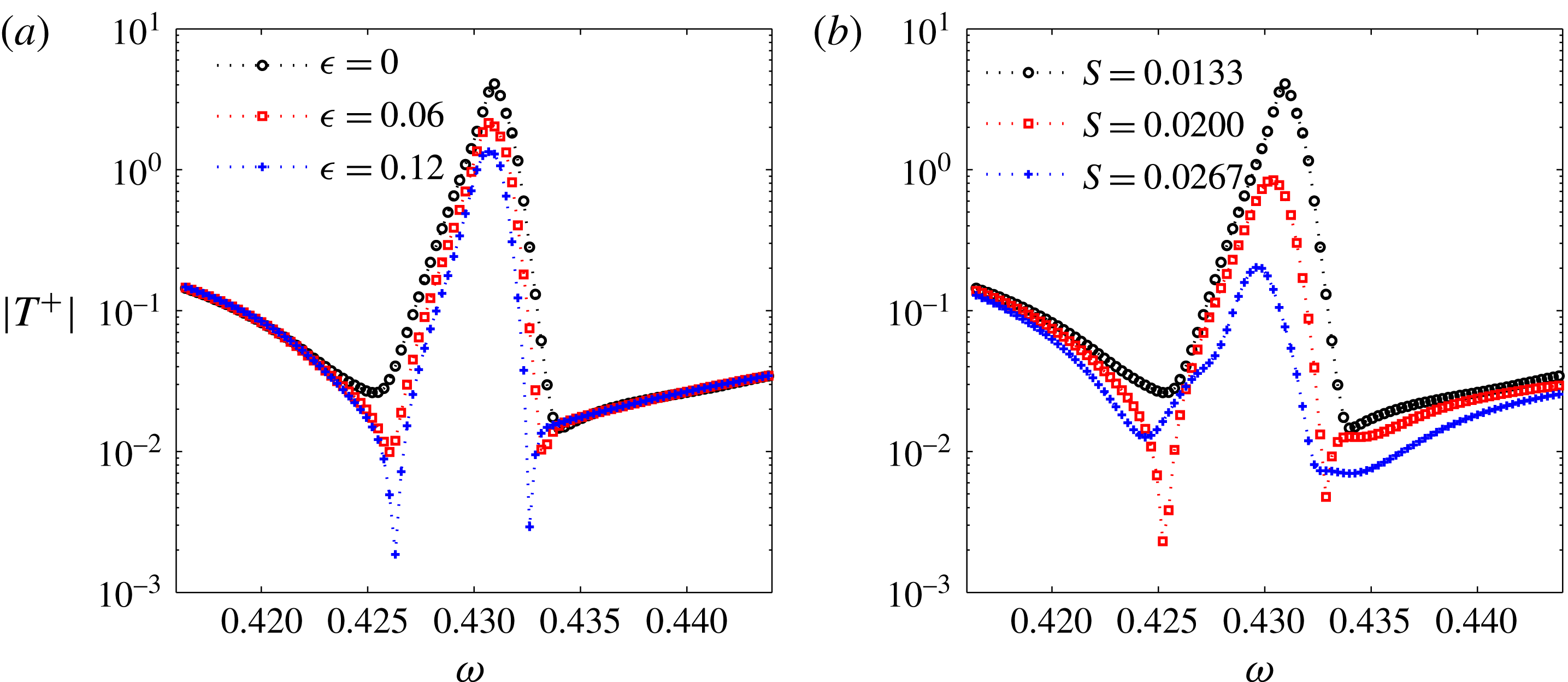
Effects of the dissipation of the hydrodynamic modes (a) and the length of spacing between the adjacent cavities (b) on the sound amplification in the periodic liner with 30 cells. In (a), the calculations are made with the default geometrical parameters but different artificial damping factor
 $\unicode[STIX]{x1D716}$
. In (b),
 $\unicode[STIX]{x1D716}=0$
, while the length of spacing
 $S$
is varied.
In a case where each periodic cell consists of two cavities of different depths, it is shown that a small depth difference can completely suppress the unstable behaviour above the liner. A homogenized approach can also correctly model the hydrodynamic instability in this case and it reveals that, for the Bloch mode stabilization, increasing the depth difference is equivalent to increasing the resistance of the lined wall.
Acknowledgements
Y.A. gratefully acknowledges support from the ANR international project FlowMatAc no. ANR-15-CE22-0016-01; X.D. also gratefully acknowledges support from the ANR international project FlowMatAc during his stay in France.
Appendix. Effects of the artificial damping and the spacing between cavities on sound amplification
As mentioned in § 3.1, some artificial damping has been added to the hydrodynamic modes in the calculations. To analyse its effect on propagation, we calculated
 $|T^{+}|$
of 30 cells with the same geometry but for different dissipation rates on the hydrodynamic modes of zones I and II. It is shown in figure 11(a) that an increase in the dissipation factor
 $\unicode[STIX]{x1D716}$
of the hydrodynamic waves leads to a clear reduction in sound amplification. This effect has already been observed in Marx & Aurégan (Reference Marx and Aurégan2013) and shows the importance of having dissipation to correctly predict the peak amplitude. Also, to verify that our model can explain the experimental observation that the peak is very sensitive to the percentage of open area (POA) (Aurégan & Leroux Reference Aurégan and Leroux2008), the spacing between the cavities
 $S$
has been varied and the results are shown in figure 11(b). They show that the peak value is highly dependent on the POA (division by 20 when the spacing is doubled). This effect can be interpreted as being related to the increase in coating resistance with the decrease in POA in the continuous impedance approach (see figure 7).



