1 Introduction
Natural disasters, violence outbreaks, political scandals, or sports results are examples of unexpected events that can occur during the fieldwork of public opinion surveys. Survey researchers traditionally considered that a changing context could threaten the validity of their measurement instruments. Other scholars, though, have identified these occurrences as an opportunity to identify the causal effect of these events on public opinion.
Already in 1969, The Public Opinion Quarterly published a series of articles aimed at studying the effect of unexpected events such as Martin Luther King’s assassination (Hofstetter Reference Hofstetter1969) or an explosion in Johannesburg (Lever Reference Lever1969) on multiple outcomes. More recently, the influence of the so-called identification revolution has led to a significant increase in the number of publications that exploit these unexpected events as opportunities to conduct design-based studies that can yield valid causal estimates of theoretically relevant shocks.
In this paper, we discuss the strengths and limitations of this identification strategy, which we call the “Unexpected Event during Survey Design” (UESD). In particular, we focus on the assumptions under which unexpected events can yield valid causal estimates. We discuss these assumptions and their observable and testable implications in detail. Next, we present several strategies to address potential violations of the assumptions as well as a series of robustness checks that can be used to assess and establish their plausibility. Our review of over 40 published studies that rely on this identification strategy shows a wide variation in the estimation strategies, tests and robustness checks that are performed to substantiate causal claims. While most researchers acknowledge some of the key identifying assumptions of this design, there is still no apparent consensus on the empirical strategy and the robustness checks that should be performed. Our aim is that this paper will help set a standard of good practices that should increase the credibility of causal claims based on the UESD.
We illustrate the strengths and weaknesses of the UESD through an original study of the impact of the Charlie Hebdo terrorist attacks (Paris, 01/07/2015) on satisfaction with government in France, relying on the 7th round of the European Social Survey (ESS), that was being fielded at the time of the attacks.
2 The Unexpected Event During Survey Design
We define the UESD as the research design that exploits the occurrence of an unexpected event during the fieldwork of a public opinion survey to estimate its causal effect on a relevant outcome by comparing responses of the individuals interviewed before the event  $t_{i}<t_{e}$ (control group) to those of respondents interviewed after the event
 $t_{i}>t_{e}$ (treatment group).
This identification strategy relies on the assumption that the moment at which each respondent is interviewed during the fieldwork of a given survey is independent from the time when the unexpected event occurs. The occurrence of the event should, therefore, assign survey respondents into treatment and control groups as good as randomly. Hence, a UESD study relies on the use of cross-sectional survey data in which time provides exogenous variation in a substantively relevant variable, such as exposure to some experience or information. Formally, the timing of the survey  $t$ is exploited as an instrument of exposure to the event
 $T$, the effects of which the researchers are interested in.
A crucial feature of the UESD is, therefore, that the event occurs unexpectedly, since predictable events might lead to violations of the key assumptions of this design (excludability and ignorability). Foreseeable events (e.g. an election result) might be anticipated by respondents who might change their attitudes in response to the event even before it has occurred. This could be especially problematic if certain respondents are more/less likely to anticipate the event and they are, at the same time, more/less likely to be interviewed after the event. Moreover, if an event is foreseeable, some respondents might postpone their participation in the survey and self-select into the treatment group.Footnote 1
This identification strategy has been frequently exploited to study the effects of important phenomena that cannot be directly manipulated through controlled experiments. This is, for example, the case of violent events such as the assassination of political leaders (Boomgaarden and de Vreese Reference Boomgaarden and de Vreese2007) or terrorist attacks (Perrin and Smolek Reference Perrin and Smolek2009; Metcalfe, Powdthavee, and Dolan Reference Metcalfe, Powdthavee and Dolan2011, Dinesen and Jæger Reference Dinesen and Jæger2013; Finseraas and Listhaug Reference Finseraas and Listhaug2013; Legewie Reference Legewie2013; Jakobsson and Blom Reference Jakobsson and Blom2014; Coupe Reference Coupe2017; Geys and Qari Reference Geys and Qari2017; Balcells and Torrats-Espinosa Reference Balcells and Torrats-Espinosa2018; Boydstun, Feezell, and Glazier Reference Boydstun, Feezell and Glazier2018; Silva Reference Silva2018). Researchers have also analyzed the effects of other theoretically relevant events such as political scandals (Ares and Hernández Reference Ares and Hernández2017; De Vries Reference De Vries2018; Solaz, de Vries, and de Geus Reference Solaz, De Vries and de Geus2018), protests and demonstrations (Silber Mohamed Reference Silber Mohamed2013; Zepeda-Millán and Wallace Reference Zepeda-Millán and Wallace2013; Branton et al. Reference Branton, Martinez-Ebers, Carey and Matsubayashi2015; Motta Reference Motta2018), presidential candidates’ speeches (Flores Reference Flores2018), Nobel prize awards (De Vries Reference De Vries2018), the announcement of election results and election fraud (Pierce, Rogers, and Snyder Reference Pierce, Rogers and Snyder2016), policy reforms (Larsen Reference Larsen2018), or flu epidemics (Jensen and Naumann Reference Jensen and Naumann2016).Footnote 2
Some of these events commonly analyzed through the UESD, such as terrorist attacks, should a priori be unexpected for most respondents. However, there are others that might be more foreseeable like, for example, election results or a scheduled legal demonstration. In fact, the same type of event might be unexpected in some contexts but not in others. For example, while in some cases the victory of a particular party or candidate in an election might be expected (e.g. CDU victory in the 2017 German election), in some others, the election results might come as a surprise by being more unexpected (e.g. the victory of Donald Trump in 2016 analyzed by Minkus, Deutschmann, and Delhey Reference Minkus, Deutschmann and Delhey2018). Researchers should, therefore, make a compelling argument about the plausibility of unexpectedness on a case-by-case basis.
The increasing popularity of the UESD can be attributed to its capacity to provide credible estimates of the causal effects of unexpected events on theoretically relevant outcomes. This capacity is based on three crucial features of this design. First, in contrast to standard observational survey studies, exogenous assignment to treatment and control groups increases the internal validity of the estimates as it can shield them from biases related to unobserved confounders or reverse causality. Second, the fact that the UESD relies on naturally occurring events (not manufactured by researchers) provides a level of external validity that goes well beyond what controlled experiments can offer. Third, in contrast to most analyses of the impact of events that use longitudinal data or different surveys stacked around the date of an event, UESD studies employ a single survey to focus on the immediate period of time surrounding the event, which ensures that the impact of other macro-level confounders is less of a concern. However, the absence of a true random assignment and the lack of control by the researchers also pose challenges to identification that need to be addressed upfront if this strategy is to be used to substantiate causal claims.
2.1 The UESD in Context
The UESD shares some properties with other research designs commonly used in social sciences, such as the Regression Discontinuity Design (RDD), the Interrupted Time Series (ITS) design, or event studies, which are common in economics and finance. While these research designs can provide relevant cues for the use of the UESD, this design has a range of unique features and particularities that warrant some specific methodological considerations.
Under some specific conditions, the UESD might be analogous to the RDD in which an observation is treated if the forcing or running variable exceeds some predetermined cutoff. In the case of an unexpected event occurred during the fieldwork of a survey, the running variable would be the fieldwork days when interviews took place and the cutoff the moment when the event occurred. However, there are several important differences. First, unlike the RDD, in the UESD, the receipt of the treatment is not linked to a given score of the running variable in any predetermined or known way. Moreover, in most applications of the RDD, the running variable will be substantively related to the potential outcomes and, therefore, inference will be restricted to the cases just below and above the cutoff. While in some UESD applications this might also be the case, in most of its empirical applications the specific day when a respondent is interviewed is not related to the potential outcomes, other than through the unforeseen event. As a consequence, the need to rely on narrow bandwidths (and the estimation of local effects) is generally less stringent.
The UESD also bears some resemblance to the ITS design (St. Clair, Cook, and Hallberg Reference St. Clair, Cook and Hallberg2014). This design, commonly used in epidemiology and health policy, is based on repeated measurements of an outcome (e.g. hospital admissions) for the same units before and after a given intervention (e.g. the approval of a policy). The measurements before the intervention are used to build expectations on the outcome trend in the absence of the intervention. An effect is identified if the postintervention observations deviate significantly from this counterfactual trend.
The core challenges to causal identification in the ITS design are related to the aggregated and time-series nature of the data: the presence of seasonality, temporal autocorrelation, and time-varying confounders. While in some cases ITS designs have been applied to the analysis of survey data, these data were recorded or used at the aggregate level (see e.g. Tiokhin and Hruschka Reference Tiokhin and Hruschka2017). In these examples, the (often few) respondents interviewed each specific day (or period) of the fieldwork are treated as a measurement of the same unit and, therefore, the data set is essentially a time series. The reduced number of daily observations might create a problem of high variance and, depending on the organization of the fieldwork, also of bias in the measurements. In the examples we discuss in this paper, the survey data is primarily analyzed at the individual level, so we do not deal with repeated measurements of the same unit but with different observations in the pre- and postevent periods. This is the core difference between the ITS and the UESD designs, and it has implications for the type of concerns and threats to identification as well as for the estimation strategies.
On similar grounds, one could also mention event studies used in finance, which analyze the behavior of firms’ stock prices in response to corporate events (MacKinlay Reference MacKinlay1997). But, again, the nature of the data used in the UESD and the comparison across different units interviewed before and after the event makes the UESD a distinct type of research design.
3 Assumptions and Threats to Causal Identification
The identification of valid causal estimates based on the comparison of respondents interviewed before and after the day of the event  $t_{e}$ hinges on several identifying assumptions. Arguably, there are two key and potentially problematic assumptions in this design.
The first one is excludability: any difference between respondents interviewed before and after the event shall be the sole consequence of the event. That is, the timing of the interview  $t$ should affect the outcome variable
 $Y$ only through the event
 $T$. In the case we are dealing with, together with the theoretically relevant event, other things could happen that make the pre- and postevent contexts different and, therefore, influence the respondents’ outcome.
The second key assumption is temporal ignorability: for any individual, the potential outcomes must be independent from the moment of the interview. Therefore, assignment to different values of time  $t$ should be independent from the potential outcomes of
 $Y$. This means that, in order to obtain an unbiased estimator, selection of the moment of the interview should be as good as random.Footnote 3
3.1 Excludability
To estimate the causal effect of the event, one must assume that the timing of the survey interview does not affect the outcome through any other channel except for the event of interest. Any factor, other than the event itself that correlates with time can potentially bias the causal estimates. We consider three potential threats to the exclusion restriction: collateral events, simultaneous events, and unrelated time trends. We also discuss another particular case in which the exclusion restriction might be violated: the endogenous timing of the event.
3.1.1 Collateral Events
We define collateral events as the succession of reactions triggered by the unexpected event of interest. For example, in the case of a terrorist attack, generally, the government will issue public statements and adopt specific policy responses. The opposition then will decide whether to back the government or criticize it for the security failure, and the news media will shape the width and tone of the coverage.
All these reactions and counter-reactions, rather than the unexpected event per se, might drive the public opinion’s response. This can be seen as a problem of an imprecise treatment. Under these circumstances, it is impossible to narrowly interpret the effect as a consequence of the event itself, and it should rather be interpreted as the joint effect of the event and the subsequent reactions. In fact, it is often legitimate to question, counterfactually, if we would observe the same effect on  $Y$ had some of these collateral events not occurred.
In some applications, the presence of collateral events might not be a problem because the event did not spur any relevant reactions, because the reactions are a constitutive characteristic of the class of events being analyzed, or because they are part of the researchers’ focus of interest. However, they often pose a generalizability problem: the estimated causal effect of the event (e.g. a specific terrorist attack) may not be generalizable to the class of events of the same type (e.g. terrorism in general) had the collateral events been different. In such cases, it may be advisable to analyze additional events of the same class to average out the specificities of each individual event (see e.g. Balcells and Torrats-Espinosa Reference Balcells and Torrats-Espinosa2018 analysis of multiple terrorist attacks).
3.1.2 Simultaneous Events
A potentially more troublesome situation can arise when other, unrelated, events take place at the same time. This might pose a problem of compound treatments, which violates the Compound Treatment Irrelevance Assumption.Footnote 4 Applied to the UESD, this assumption implies that out of all the treatments that covary with the timing of the interview, the event of interest is the only treatment that affects the potential outcomes. If, instead, there are reasons to believe that any of these other events might have had an effect on the outcome of interest, the exclusion restriction would be violated. For example, the 2016 Nice terrorist attack in France took place during Bastille Day celebrations, so any effect on a political outcome might be caused both by the attack and the national commemoration.
Unlike the case of collateral events, this problem cannot be reduced to an issue of precision, interpretation, and generalizability of the treatment effects. It is true, however, that in most existing applications of the UESD the events analyzed were highly salient episodes. Therefore, it is often unlikely that the observed effect would have been driven by other, relatively minor events that were not nearly as salient.
3.1.3 Unrelated Time Trends
Another violation of the exclusion restriction can be generated by the presence of time-varying variables that, aside from the event itself, are systematically related to the outcome (temporal stability assumption). Let  $t$ be a continuous time variable and
 $T$ a dichotomous variable that takes value 1 if the respondent was interviewed after the event and 0 otherwise. In the presence of a monotonic effect of
 $t$ on
 $Y$, many arbitrary partitions of
 $t$ will yield statistically significant effects in the same direction as the preexisting trend. Time trends can exist for many different reasons, often unrelated to the unexpected event. For example, variables such as subjective well-being are related to calendar effects (Csikszentmihalyi and Hunter Reference Csikszentmihalyi and Hunter2003).
3.1.4 Endogenous Timing of the Event
A particular case in which some of the aforementioned threats to excludability can emerge is if the timing of the event is endogenous. Most unexpected events of interest are human-crafted and, therefore, an actor decides when the event takes place. For example, the precise time at which a corruption scandal breaks in the news or the moment at which a terrorist group perpetrates an attack are events that, although unexpected for almost all citizens, might be actually planned by politically motivated actors.
If the decision about the moment when the event occurs is endogenous to the outcome variable  $Y$, and therefore
 $T$ is correlated with the error term, the excludability assumption will be violated. Take, for example, the case of a partisan news media outlet. Once they receive information about a corrupt act committed by the incumbent, they might strategically manipulate the moment at which the information is disclosed in order to maximize (or minimize) damage to the incumbents’ popularity. They might, for example, break the news at a time in which another, more salient event is taking place to play a diversionary strategy and reduce the effect. If this is the case, assignment to treatment and control cannot be treated as exogenous, and, most probably, either a preexisting trend or some other events that correlate with
 $t$ are having an effect on
 $Y$.
3.2 Ignorability
Formally, the ignorability assumption states that respondents’ treatment status is independent of their potential outcomes  . However, in the UESD, assignment to the treatment and control groups is not under the researchers’ control, and is not random. Treatment assignment is the result of a combination of the unexpected event and a set of decisions related to data collection taken by the fieldwork operative.
In simple random samples with full response, all individuals would have an identical probability of being interviewed at any time during the fieldwork, before or after  $t_{e}$. A suitable setting for this to hold would be a telephone survey with random digit dialing, a simple random sampling design and full response. In this case, any temporal partition of the sample would be as good as random. However, this is seldom the case in most surveys. Another favorable survey design for the ignorability assumption to hold is the rolling cross-sectional design, used in surveys such as the National Annenberg Election Survey (NAES) or the Canadian Election Study (CES), that explicitly guarantees that the date in which each respondent is interviewed is random (Johnston and Brady Reference Johnston and Brady2002). Next, we discuss how the variation in survey sampling methods, fieldwork procedures, and the propensity and availability of sampled citizens to respond will, in most cases, lead to violations of the ignorability assumption.
3.2.1 Fieldwork Organization: Imbalances on Observables
Threats to the ignorability assumption often stem from complex sampling designs, such as cluster, stratified, or multistage samples. In these designs, the primary sampling units are often contacted and interviewed sequentially. For example, in face-to-face surveys the fieldwork often follows a geographical pattern for efficiency reasons. Respondents in area A are interviewed first, then interviewers move to area B, and so on. Any correlation between subject location and time of the interview will lead to a violation of the ignorability assumption, since the location can be correlated with many other respondents’ characteristics that might bias the findings.Footnote 5
Quota sampling is another strategy that can generate imbalances. Often the fieldwork goes on until a given quota is completed. Then, researchers seek to complete the remaining quotas and, therefore, any additional interview (or invitation to respond) will target the respondents with profiles that match the incomplete quotas. Often, there is a systematic pattern in the pace of quota completion, and the quotas corresponding to the types of respondents that are easier to reach and survey (such as inactive population that stays at home) will fill up earlier. If this is the case, timing of the interview will be correlated with respondents’ characteristics and, therefore, splitting the sample at a specific point in time might not satisfy the ignorability assumption.
When information on how the fieldwork unfolded is available, researchers can use relevant observed characteristics of the respondents (e.g. place of residence or the variables used to set up the quotas) to relax the ignorability assumption and rely on a more plausible Conditional Ignorability Assumption. This assumption states that treatment status is independent of individuals’ potential outcomes conditional on a set of covariates:  . This is similar to the common practice of observational studies in which statistical control of potential confounders is the only strategy to ensure conditional ignorability. However, in the case of the UESD, the exogenous nature of the cutoff point increases the plausibility that, once we take into account the relevant observables related to how the fieldwork was organized, treatment status is orthogonal to the potential outcomes.
3.2.2 Unobservable Confounders: Reachability
Another threat to causal identification originates from potential imbalances between the treatment and control groups on unobservable characteristics. In the context of the UESD, this is likely to be related to the different levels of reachability of sampled units. Some respondents are more elusive to survey researchers and require a greater effort to be contacted. Differences in reachability are related to respondents’ ease of contact and their inability or reluctance to participate. For example, those who are older and out of the labor market are likely to be interviewed early during the fieldwork period because they are more often at home and have fewer time constraints (Brehm Reference Brehm1993; Stoop Reference Stoop2004). Similarly, those who are more interested in the topics covered in the survey should be more willing to respond when they are first contacted (Brehm Reference Brehm1993). As a consequence, those who respond early to the survey might be different than those who respond later.
The extent to which these differences in respondents’ reachability might pose a threat for the UESD will depend on the survey design. For example, in the case of rolling cross-sectional designs, confounders related to reachability should be less of a concern since this design guarantees that the day when respondents are interviewed is, in principle, random. In any survey in which the sampled units have any possibility to opt into the survey at different points in time, though, reachability will lead to differences between those who are interviewed early and late. Take as an example an online survey in which a link is distributed among all the sampled units and respondents can decide when they answer the survey (within a specified time frame). Biases related to reachability can also arise due to the common practice of making repeated attempts to recontact and interview sampled households/individuals that were not found or refused to cooperate when they were first contacted. Footnote 6
We illustrate this point through the 2014 round of the ESS, a survey in which substitution of sampled units is not allowed and, therefore, interviewers make repeated attempts to contact nonresponding units.Footnote 7 Figure 1 summarizes the relationship between the number of attempted contacts with sampled units and the time during the fieldwork when these units were finally interviewed. In 17 out of the 21 countries included in the ESS, this relationship is positive and statistically significant. In most cases, the higher the number of contact attempts needed to survey a subject, the higher the likelihood that she will be interviewed later during the fieldwork. Therefore, the subjects who are more elusive and harder to reach will have a higher probability of being interviewed after any unexpected event. If reachability is correlated with the potential outcomes, its correlation with treatment assignment will bias the estimates of the causal effect.
To exemplify the potential biases that the differential reachability of respondents might generate, in table A.1 in the Supporting Information we assess the relationship between the timing of the interview and respondents’ observable characteristics in the ESS. As expected, those who were older, less educated, and out of the labor market (unemployed, retired, or doing housework) were interviewed earlier during the fieldwork of this survey. In contrast, when we conduct a similar analysis with the 2015 rolling cross section of the CES and the 2008 NAES, the respondents’ characteristics appear to be less related to the timing of their interview. However, even in these surveys, interview timing is related to some demographic characteristics of respondents (see Section A2 in the Supporting Information for a discussion of these findings). Therefore, it is advisable to always account for potential biases related to reachability, even in the a priori most favorable sampling conditions.
Number of attempts to survey before interview completion and day of fieldwork when interview was completed. Note: Kernel-weighted local polynomial smoothing with 95% confidence intervals. Coefficient and  $t$-statistic of OLS model regressing fieldwork day when interview was completed on the number of attempts to survey.

3.2.3 Attrition
Survey research suffers from severe and increasing problems of nonresponse (Berinsky Reference Berinsky2017). This is particularly problematic when nonresponse is correlated with potential outcomes. In UESD studies, this might be even more troublesome if nonresponse is triggered by the treatment. As a result of being exposed to certain events, some people might become more likely to refrain from responding to particular survey questions (item nonresponse) or even be less likely to participate in surveys altogether (unit nonresponse). The opposite can also happen when events unevenly increase the willingness of particular individuals to respond. In such cases, the general problem of nonresponse being correlated with the outcome is aggravated as this correlation might be, in turn, different in the treatment and control groups. Take, as an illustration, the example of a coup that topples an autocratic government. There would be reasons to believe that individuals with certain political preferences—correlated with the outcome variable of interest—are now more (less) likely to respond to the survey than they were before. Differences in  $Y$ between both groups might reflect the substantively relevant effect of the event itself and, also, the fact that different types of people are responding to the survey.
3.3 Noncompliance
So far, we assumed that all respondents interviewed after the event were exposed to it (full compliance). Assignment to the treatment group  $t_{i}>t_{e}$ was assumed to perfectly correspond to actually receiving the treatment
 $T=1$. In most existing applications of the UESD, this is a plausible assumption, since they refer to highly salient events.
In some cases, though, some subjects assigned to the treatment group might not be actually exposed to the event due to lack of direct experience or lack of access to information. This is potentially relevant in applications of the UESD in which the events are not extremely salient, for example, Nobel Prize awards (De Vries Reference De Vries2018). Under these circumstances, we would be facing a problem of one-sided noncompliance, in which some of the subjects are never-takers: despite having been assigned to the treatment group  $t_{i}>t_{e}$, they did not receive it (
 $T=0$). Since exposure to information or direct experience with the event might be correlated with potential outcomes, in the presence of this type of noncompliance, the difference between the subjects interviewed before and after the event (
 $Y_{i}(t_{i}>t_{e})-Y_{i}(t_{i}<t_{e})$) cannot be interpreted as the average treatment effect (ATE).
3.4 Heterogeneous Effects and Posttreatment Bias
UESD studies commonly present heterogeneous effects as their central findings. This is often for good reasons, as these will be the theoretically relevant effects: the unconditional effect of an event might be of little theoretical interest. Moreover, the heterogeneous effects are often relevant to shed light on the causal mechanisms at work.
While general concerns about the causal interpretation of heterogeneous effects in experimental research might apply here (Stokes Reference Stokes2014), in the case of the UESD special attention should be paid to potential posttreatment biases (Montgomery, Nyhan, and Torres Reference Montgomery, Nyhan and Torres2018). In cross-sectional surveys, the conditioning variables will always be measured after the event has occurred for the treatment group. While it is unlikely that some of the variables that could be used as moderators (e.g. gender or age) are affected by an event, many other theoretically relevant moderators could be shaped by it. If this is the case, the estimation of heterogeneous effects can be biased.
Think, as an illustration, of a study about the impact of a terrorist attack on trust in government, which tests whether the effect is different among those who identify with the incumbent party. In the unconditional comparison, the respondents interviewed before the attack might represent a valid counterfactual. However, once we condition for party identification, we compare those that identified with the party in government before the attack and those that identify with it in spite of or because of the attack. If the attack had an effect on government support, the group of government identifiers (the moderator variable) would be different before and after the event, and, therefore, the estimate would not have a valid causal interpretation.
4 Estimation and Assessment of Assumptions
In the absence of threats to ignorability and excludability, a difference in means between the groups interviewed before and after the event would yield an unbiased estimation. However, this naive approach ignores the potential violations of these assumptions. Next, we propose a series of best practices in the form of various estimation strategies and robustness checks that can be used to lend credibility to the causal estimates.
4.1 Event Description and Qualitative Assessment of Assumptions
In-depth background knowledge is fundamental in order to validate the ignorability and excludability assumptions. A close and substantive examination of the event itself, of the circumstances surrounding it, and of the survey instrument should be the first step in any UESD study. Quantitative information will often prove useful for this, but researchers need to acquire in-depth case-based knowledge focused especially on the macro-level dynamics that generated the event and assigned units into treatment (see Kocher and Monteiro Reference Kocher and Monteiro2016).
4.1.1 Event Characterization
To understand the process of treatment assignment, the event should be thoroughly characterized, paying special attention to its timing and salience. Assessing the salience of the event is of utmost importance to assess the likelihood of noncompliance. The circumstances and causal chain leading to the event should also be discussed, paying special attention to the need of assessing and validating the definitional claim of the unexpected nature of the event. This examination should also address the possibility that, even if unexpected for most citizens, the event could have been strategically timed. Researchers should also describe the reactions that it generated in order to understand the role of collateral events.
Contextualizing the event and describing the circumstances surrounding its occurrence is also relevant in order to rule out the presence of other, simultaneous, events that might confound the effect of time. Sources such as Internet search trends and an analysis of print media can provide valuable evidence about the salience of the event and the potential presence of simultaneous events that could confound the estimation.
4.1.2 Background Information on the Survey
Detailed background knowledge about how the survey was conducted is also relevant to understand the process by which units are assigned to treatment. Special attention should be paid to the sampling procedure, the procedures to contact sampled units, and strategy to deal with unit nonresponse. In the case of multistage sampling and/or quota sampling, researchers must collect information about how the fieldwork unfolded, because that might create systematic differences in the type of respondents that are interviewed before and after  $t_{e}$. In the case of disruptive events, one should also check if the event generated any changes in the fieldwork organization. Researchers must also assess if the procedures for recontacting individuals or for refusal conversion might produce systematic biases, especially if refusal conversion strategies start at a specific point in time during the fieldwork. All these questions should be discussed in relation to the way in which the survey is administered—either in person, by phone, mail, or online—as each of these methods will have particularities when it comes to the procedures to contact and recontact sampled units.
4.2 Assessing and Addressing Violations of the Ignorability Assumption
4.2.1 Balance Tests
To assess the plausibility of the ignorability assumption, one can analyze balance on pretreatment covariates between treatment and control groups. A difference of means between them provides information on whether assignment to treatment and control is statistically independent of these covariates. If imbalances appear in characteristics related to the outcome of interest, this might generate a statistical dependence between treatment assignment and the average outcome. Case-specific considerations should drive the decision of which covariates to include in these tests. Usually, one would consider the sociodemographic characteristics of respondents as well as their place of residence (e.g. region, municipality, etc.).
4.2.2 Bandwidths and Statistical Power
Selecting the appropriate bandwidth is of central concern in the literature on Regression Discontinuity (Imbens and Lemieux Reference Imbens and Lemieux2008). Generally, in most RDD applications, the bandwidth will be as narrow as possible, given that the forcing variable is substantively related to the potential outcomes. In the UESD, the equivalent to the RDD forcing variable is the timing of the interview and, in most applications, will not be related to the potential outcomes. Therefore, individuals interviewed around the day of the event will not necessarily be more similar to each other, and narrower bandwidths will increase variance (reduce  $N$ and statistical power), but not necessarily reduce bias. There are other downsides to the use of narrow bandwidths. First, they might compromise the generalizability of the results as the effects will tend to be very local. Second, the effects of certain types of events can take some time to unfold, and a narrow bandwidth might miss part of the effect or even lead to a false negative. All these considerations should be taken into account when deciding on the appropriate bandwidth of days considered around the event date.
Under certain conditions, though, narrower bandwidths might reduce bias. In the presence of time trends, collateral events or confounders correlated with time of the interview, the UESD will present an analogous situation to the RDD. In these cases, and especially in surveys with prolonged fieldworks, researchers can narrow down the bandwidth  $h$ around the cutoff point and only use respondents interviewed during a certain period before and after the event to increase the plausibility of the ignorability assumption, and the exclusion restriction. In these situations a narrower bandwidth could be an effective way of achieving conditional independence, since the potential outcomes of those interviewed around the day of the event should be more likely to be independent from treatment assignment:
 , where
 $h_{i}$ is unit’s
 $i$ absolute distance (in days) from the day when the event took place. Therefore, in some cases, narrower bandwidths might provide an effective way to substantiate the as-if random treatment assignment assumption for that specific subset of the sample. Narrower bandwidths can also reduce the probability that other events or time trends drive the estimated effects. Narrower bandwidths should, therefore, be presented as a robustness check whenever possible. In surveys with prolonged fieldwork, where there is a greater potential for a correlation between the time of the interview and potential outcomes, this might even become the primary estimation strategy.
When conducting this robustness check, or when estimating the effects with a subsample around the event date, one should always consider the trade-off between narrower bandwidths and statistical power. In the UESD, the sample is always split into pre- and postevent subgroups. As a consequence, the power of statistical tests is lower, and the study can be underpowered. This is especially the case if we are dealing with small samples, when the event occurs early/late during prolonged fieldworks, or when narrowing the bandwidth of days considered around the event date. Therefore, in all UESD studies, but especially in these cases, we recommend conducting power analyses to determine how many cases in the control and treatment groups would be adequate in order to detect a meaningful effect in each specific case. Hence, when discussing results based on multiple bandwidths, we recommend a graphical representation that, beyond the effect estimates, summarizes for each bandwidth the number of units included in the treatment and control groups and their corresponding statistical power (for meaningful effect sizes).
4.2.3 Covariate Adjustment
The UESD might not always satisfy the ignorability assumption, even after narrowing the bandwidth around the date of the event. Therefore, to satisfy the Conditional Ignorability Assumption, one can either preprocess the data through matching techniques to improve covariate balance between treatment and control groups and/or use controls in a regression framework. Matching techniques might be preferable in most situations, as they make less assumptions on the functional form of the relationships, and in some cases, such as the entropy balancing method (Hainmueller Reference Hainmueller2012) can balance the mean, variance, and skewness of the covariates across groups.
This is a quite common practice in the literature. However, it is important to carefully select the covariates  $X_{i}$ that are included in the analyses. The covariates
 $X_{i}$ used will generally be the same as those included in the balance tests. It is very important also to consider all those covariates that can take into account the survey design and the unfolding of the fieldwork, such as those related to the reachability and place of residence of respondents, as well as to their willingness to participate in the survey process. In the case of surveys using quota or stratified samples, researchers must consider all the variables that are used to establish the quotas or strata. However, it is also important to pay attention to the covariates that shall be avoided. In the UESD, all covariates are measured posttreatment, so variables that can be potentially affected by the event should not be included to avoid posttreatment bias (Montgomery, Nyhan, and Torres Reference Montgomery, Nyhan and Torres2018). For example, in studies analyzing the effects of a scandal on the attitudes toward the incumbent (e.g. Ares and Hernández Reference Ares and Hernández2017), researchers might wish to include a covariate measuring if respondents identify with that party. However, precisely as a result of the scandal, respondents might be less likely to identify with the incumbent party, and introducing such a covariate could generate posttreatment bias.
4.2.4 Attrition
Events might alter respondents’ likelihood of providing a valid answer to the questions measuring the outcome of interest (item nonresponse). Differences in the proportion of respondents who offer a don’t know answer or refuse to answer the question measuring the outcome of interest across the control and treatment groups should be analyzed. If that is the case, researchers should carefully investigate whether there is any particular group of respondents that has modified their nonresponse pattern.
Events might also alter individuals’ likelihood of responding to the survey altogether (unit nonresponse). Analyzing unit nonresponse patterns before and after the event poses greater challenges, as it requires access to survey paradata containing information about the moment when nonrespondents were contacted. If this is available, one can first assess if the event affects the rates of failed interview attempts. However, a higher rate of unit nonresponse after the event might just reflect the fact that as the fieldwork progresses, survey operatives are more likely to recontact those who are more difficult to reach or less willing to participate in the first place. Likewise, similar rates of nonresponse before and after the event might still pose a problem for causal identification if the profiles of nonrespondents are different. A comparison of the characteristics of nonrespondents before and after the event will provide valuable clues as to whether the event might have altered the likelihood of participating in the survey for a particular group.
4.3 Assessing and Addressing Violations of the Exclusion Restriction
The exclusion restriction implies that the timing of the survey only affects the outcome of interest through exposure to the event. The most relevant threats to this assumption are generated by simultaneous events and preexisting time trends. One can assess the plausibility of this assumption through falsification tests, which test for the presence of an effect of the event and of the timing of the survey where it should not exist.
4.3.1 Inspection of Preexisting Time Trends
To address the possibility that preexisting time trends, unrelated to the event of interest, could bias the findings, researchers can test for the existence of such a trend before the event took place. Placebo treatments constructed at arbitrary points at the left of the cutoff point ( $t_{p}<t_{e}$) should not affect the outcome. We follow the RDD literature and suggest to split the control group subsample at its empirical median and test for the absence of an effect at that point (Imbens and Lemieux Reference Imbens and Lemieux2008). This strategy has the advantage of producing control (
 $t_{i}<t_{p}$) and treatment placebo (
 $t_{p}<t_{i}<t_{e}$) groups with a similar number of respondents. More generally, it is also advisable to examine the relationship between the timing of interviews and the outcome variable all throughout the preevent period, to check that these two variables are not systematically related during that period.
4.3.2 Falsification Tests Based on Other Surveys or Units
Researchers can also conduct falsification tests that increase the plausibility of the excludability assumption by relying on other surveys. Many surveys are repeated periodically. This provides the opportunity for conducting a falsification test of the effect of a placebo event that occurs on the same date as the event of interest but, for example, one year before/after it. These tests can help rule out that the effects of the event of interest are caused by aspects related to the timing of the survey fieldwork or to any other cyclical trends.
If the effects of the event of interest should be restricted to a specific region or country and contagion effects can be theoretically ruled out, one can also conduct placebo tests that exploit this circumstance. Surveys are generally conducted at the same time in different regions of a country or, also, in different countries. If this is the case, researchers can use these units as additional counterfactuals by testing for the effect of the event in a location where it should not exist (see Pollock et al. Reference Pollock, Barabas, Jerit, Schoonvelde, Banducci and Stevens2015). This test can be used to rule out that a global time trend or any other simultaneous event that might be affecting the outcome of interest in different countries or regions bias the causal estimates. This of course does not apply to cases in which global or contagion effects are to be expected (see Legewie’s Reference Legewie2013 study of the impact of a terror attack on citizens’ attitudes toward immigrants in various distant countries).
4.3.3 Effects of the Event on Other Outcome Variables
One relevant threat for the excludability assumption is the occurrence of simultaneous events. While a thorough qualitative analysis will be useful to assess the plausibility of the assumption, researchers can also conduct falsification tests that involve testing for the effect of the timing of the event on variables that, theoretically, should not be affected by it.
The crucial question here is how to select these variables. Recall that  $t$ (timing of the interview) is an instrument for the event
 $T$, and therefore it should only affect
 $Y$ through
 $T$. If one suspects that another event
 $T^{\prime }$ is driving the effect, a good falsification test would imply looking for an alternative outcome
 $Y^{\prime }$ that is theoretically unrelated to
 $T$ but susceptible of being affected by other events
 $T^{\prime }$ that might also have an effect on
 $Y$. Therefore, ideally, one would like to have variables that are as close as possible to
 $Y$ except for the fact that we should expect them not to be affected by
 $T$. If we find an effect of
 $t$ on
 $Y^{\prime }$, this might be an indication of a violation of the exclusion restriction. While this test might lend additional plausibility to assumption, it is not, by itself, either necessary or sufficient to rule out the possibility that the estimated results for
 $Y$ are being driven by another event.
4.4 Assessing Compliance
The one-sided noncompliance problem discussed above refers to the situation in which the subjects in the treatment group have not been exposed to the treatment. In the UESD framework, all respondents interviewed after the event will be exposed, provided that they were aware of it. Unfortunately, this is not directly testable as the unexpected nature of the event of interest means that survey questionnaires will not include specific manipulation checks.
However, sometimes one can rely on indirect pseudo-manipulation checks. Salient events often have an impact on the types of problems that respondents perceive to be important in their countries, and this might be reflected in their responses to the “most important problem(s)” questions, which are routinely asked in public opinion surveys (see e.g. Boomgaarden and de Vreese Reference Boomgaarden and de Vreese2007). If this is the case, a perceptible increase in the salience attributed to the problems to which the event is related should be observed for all types of respondents, regardless of their pretreatment characteristics.
If noncompliance is a real possibility, the difference between the treatment and control groups should be interpreted as an intent-to-treat (ITT) effect, rather than as an ATE or an average treatment effect on the treated (ATT). The subjects in the group interviewed after the event “have been given the opportunity” to receive the treatment, but often we cannot be entirely certain that they have been effectively exposed to it, and, thus, the interpretation as an ITT seems more appropriate. This is especially important for less salient events or in poor information environments, where the likelihood of noncompliance is higher.
4.5 Summary
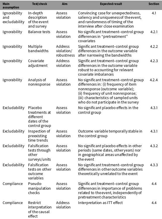
Tests and robustness checks to assess and address violations of assumptions.

In Table 1 we summarize the strategies that applied researchers can implement to assess the plausibility of these assumptions and, eventually, address some of their most common violations. Our analysis of these potential violations advises caution in the causal interpretation of the effects. In any UESD, special attention should be paid to the assessment of the observable implications of the ignorability and excludability assumptions and, in all instances, studies should conduct robustness checks that can help rule out some of the key violations of these assumptions. The list of strategies in Table 1 should be read as a series of best practices to be followed whenever possible, and not as a checklist for each and every UESD study. Often they will not be relevant or possible to conduct. Take, for instance, Kim and Kim’s (Reference Kim and Kim2019) analysis of the impact of a public statement on the diffusion of a rumor, where a “pseudo-manipulation check” would overlap with the estimation of the main effect on the outcome variable.
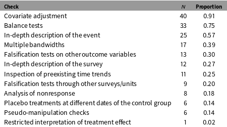
Table 2 presents an overview of the empirical strategies and robustness checks conducted in published UESD studies.Footnote 8 The table reveals a high degree of heterogeneity in the empirical strategies implemented in existing UESD studies. While most authors conduct balance tests and some form of covariate adjustment, the use of other robustness checks and strategies to assess and substantiate the observable implications of the assumptions of this research design are far less common.
5 Empirical Application: The Charlie Hebdo Terrorist Attacks and Satisfaction with Government
We illustrate the use of the UESD through an analysis of the effects of the Charlie Hebdo terrorist attacks on individuals’ satisfaction with government in France. While terrorism can affect political attitudes in countries other than those directly targeted (Legewie Reference Legewie2013), we restrict the illustration to France, where according to the well-established “rally round the flag” hypothesis (see Hetherington and Nelson Reference Hetherington and Nelson2003), we can expect a positive impact of these attacks on government approval.
The Charlie Hebdo terrorist attacks occurred in Paris at approximately 11:30 a.m of January 7th, 2015. As a result of the attacks, 12 people related to the Charlie Hebdo satirical magazine were killed. On January 8th, four hostages were also killed in a related incident involving an acquaintance of the Charlie Hebdo attackers. The two Al-Qaeda terrorists that perpetrated the Charlie Hebdo attack were shot and killed by the police on January 9th. The attacks were followed by large-scale demonstrations, which gathered citizens and politicians from all parties, as well as international leaders. These attacks coincided with the fieldwork of the 7th round of the ESS in France, which was in the field between October 31st, 2014 and March 3rd, 2015.Footnote 9
Empirical strategy and robustness checks of 44 published studies.

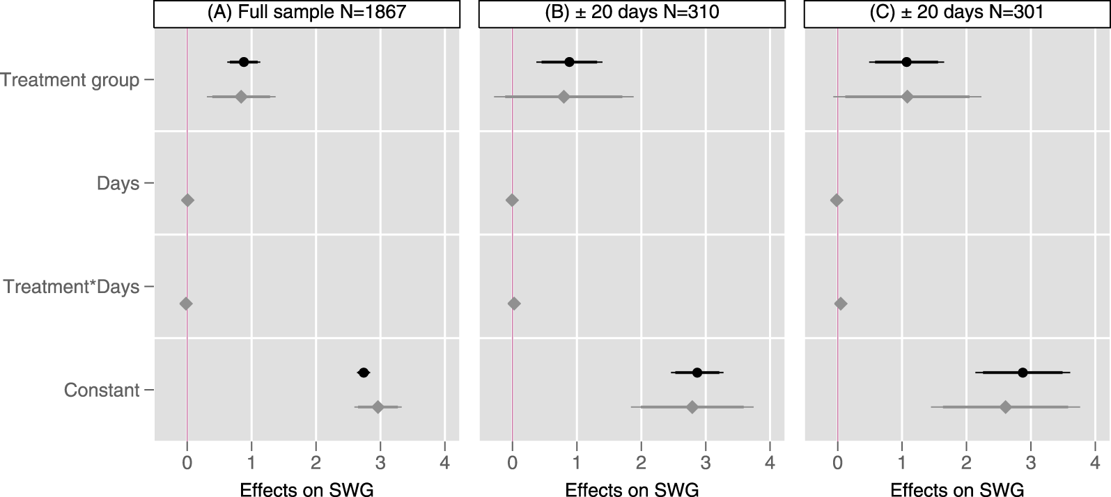
Effects of Charlie Hebdo attacks on satisfaction with government (SWG). Note: Black spikes (circle markers) summarize results from OLS models that only include the treatment indicator. Gray spikes (diamond markers) summarize the results of models that include an interaction between the treatment indicator and the running variable measuring fieldwork days. Thick and thin lines are 90% and 95% confidence intervals, respectively. The models summarized in Panel C are estimated with entropy balancing weights and region fixed effects.

We exemplify the use of the UESD through this event for three reasons. First, terrorist attacks are the type of events most often analyzed through the UESD. Second, the “rally round the flag” theory lead us to expect that satisfaction with government should increase in the aftermath of the attacks. Third, the ESS provides extensive documentation and complementary data that allow us to illustrate a series of good UESD practices.
5.1 Naive Baseline Estimation
Panel A in Figure 2 summarizes the naive baseline estimation of the effects of the Charlie Hebdo attacks on individuals’ satisfaction with government, which is measured on a 0–10 scale. Since the event took place on January 7th at 11:30, we exclude all those interviewed during that day from the analyses. Therefore, the treatment group variable takes the value 0 for those interviewed before January 7th and the value 1 for those interviewed after that day.
The results of an ordinary least squares (OLS) model that only includes the treatment indicator (black spikes and circle markers in Panel A) indicate that those interviewed after the attacks were more satisfied with the national government. The effect of the attacks is substantial, since a 0.88 average increase in satisfaction with government corresponds to a change of almost half a standard deviation on the pretreatment distribution of the satisfaction with government variable.
Next, we estimate if this change in satisfaction with government occurred immediately after the Charlie Hebdo attacks. For this purpose, we specify a model that includes a running variable ranging from -68 to 46 (the fieldwork days before and after the attacks), with 0 corresponding to January 8th. This variable is interacted with the treatment indicator. In this interactive model, the constitutive term for the “treatment group” variable corresponds to the effect of the terrorist attacks when the running variable “days” equals 0 (i.e. on January 8th, the first day immediately after the attacks). The interactive term, in turn, indicates whether or not the effects of the attacks changed (weakened or strengthened) as time went by after the attacks. The “treatment group” coefficient in the interactive model (gray spikes and diamond markers in Panel A of Figure 2) reveals that the levels of satisfaction with government increased immediately after the attacks. Moreover, the interactive term of this model indicates that the effects of the attacks did not significantly change thereafter (see Finseraas and Listhaug Reference Finseraas and Listhaug2013 for a similar finding about the effects of terrorist attacks on fear of terror).
While all these results are in line with the “rally round the flag” hypothesis, we cannot interpret them causally unless we assess whether the key identifying assumptions of the UESD are met.
5.2 Balance Tests, Bandwidths, and Covariate Adjustment
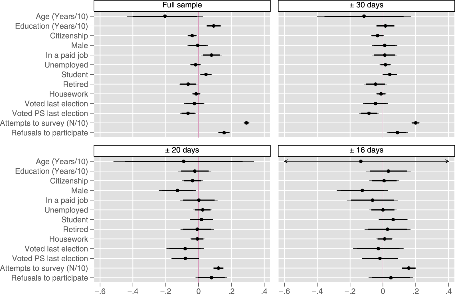
In Figure 3 we summarize the covariate imbalances between treatment and control groups using multiple bandwidths. In the balance tests we include the sociodemographic characteristics of respondents and two retrospective variables measuring if the respondent voted in the last election and if she voted for the party in government (PS). In addition, we also include two variables from ESS paradata related to the reachability of respondents: the number of times that an individual was contacted before the completion of the survey interview and the number of times she refused to participate.
Balance tests: covariate differences between the treatment and control groups. Note: Entries report the difference in the mean of the covariates between the treatment and control groups. Thick and thin lines are 90% and 95% confidence intervals, respectively.

In the full sample, the treatment and control groups are unbalanced in several pretreatment covariates. Those in the treatment group were harder to reach, younger, more educated, more likely to be either employed or studying, and less likely to support the party in government. By narrowing the bandwidth, these imbalances are substantially reduced.Footnote 10
To conduct our analyses of the Charlie Hebdo attacks, we rely on the  $\pm 20$ days’ bandwidth for several reasons. First, the balance tests indicate that relying on a wider bandwidth leads to larger imbalances in pretreatment covariates. Second, our assessment of the aftermath of the attacks indicates that until January 25th the French media coverage was clearly dominated by news related to the attacks. Third, the
 $\pm 20$ bandwidth provides sufficient statistical power to detect a meaningful increase in satisfaction with government (equivalent to one-third of the standard deviation of this variable in the control group).Footnote 11
The effects of the terrorist attacks drawing on the  $\pm 20$ bandwidth are summarized in Panel B of Figure 2. Results indicate that the average level of satisfaction with government was significantly higher after the attack. Moreover, the interactive model (gray spikes) suggests that the boost in satisfaction occurred immediately after the attack, although, in this case, the “treatment group” coefficient does not reach conventional levels of statistical significance.
Regarding covariate adjustment, we rely on entropy balancing to preprocess the data and produce covariate balance between the treatment and control groups by re-weighting units appropriately (Hainmueller Reference Hainmueller2012).
To re-weight the observations, we consider all covariates  $X_{i}$ included in the balance tests, with the exception of the variable measuring the number of attempts to survey and the respondent’s region of residence.Footnote 12 When re-weighting the sample through entropy balancing and including region fixed effects, the average effect of the Charlie Hebdo attacks is of 1.07 (Panel C in Figure 2). Moreover, the “treatment group” coefficient of the interactive model indicates that the average increase in satisfaction with government was almost of the same magnitude immediately after the attacks.
5.3 Additional Robustness Checks
In the Supporting Information, we conduct a set of analyses to assess the plausibility of the temporal stability assumption through a placebo treatment (table D.3), analyze the relationship between the timing of interviews and the outcome variable during the whole survey fieldwork period (Figure D.9), rule out that the attacks caused a problem of attrition (Tables D.4 and D.5), perform falsification tests based on other rounds of the ESS to rule out that the identified effects are driven by seasonal trends (Figure D.10), and assess the threat posed by simultaneous events through falsification tests using alternative outcomes (Figure D.11).Footnote 13
6 Concluding Remarks
In this paper, we have described and systematized the UESD, focusing on the assumptions under which unexpected events that occur during the fieldwork of surveys can yield valid causal estimates. The impact of political events on public opinion can be analyzed through different designs. For example, one can correlate the recall of an event (or the importance attributed to it) and the outcome of interest through a cross-sectional survey. However, this empirical strategy is likely to be affected by endogeneity biases. Longitudinal studies with repeated observations of the same individuals can overcome some of these biases. Yet, in these studies, the outcomes of interest are often measured a long time after the event occurred. This might lead to an underestimation of the effects and a greater potential for bias due to the occurrence of other unrelated events. Priming survey experiments are an alternative in which researchers have full control over treatment assignment and administration. Therefore, they are more immune to the type of threats discussed here. However, they are generally based on artificially designed treatments and subject to potentially short-lived effects (Gaines, Kuklinski, and Quirk Reference Gaines, Kuklinski and Quirk2006), which may raise concerns about their external validity (Barabas and Jerit Reference Barabas and Jerit2010). The UESD, this paper has argued, can be a compelling alternative, provided its key assumptions are shown to hold.
One of the drawbacks of most UESD studies is that they are event specific, and this can limit the generalizability of the findings. Each event is in some regards unique. With a single-event study we cannot rule out the possibility that the estimated effect is driven by one of its specific characteristics or by collateral events. This can be addressed if the timing of collateral events allows for a separate estimation based on the change in the outcome of interest at the exact time in which the event took place. However, this is not always possible or advisable. Therefore, it is always necessary to discuss how the event analyzed might deviate from a typical case of that class of events.
The ideal way to increase the generalizability of UESD studies is to analyze more than one event of the same class in order to establish some regularities (e.g. Legewie Reference Legewie2013). However, this alternative will often not be feasible simply because no other event of the same class coincided with the fieldwork of a survey. A good alternative in these cases is to complement UESD studies with lab or survey experiments, which can be designed to study the effect of a similar event in isolation (e.g. Flores Reference Flores2018).
One question that remains is whether surveys with a short or prolonged fieldwork are more adequate to conduct UESD studies. The main benefit of a prolonged fieldwork is that one can assess in detail the existence of preexisting time trends. However, when compared to shorter fieldworks, they have clear drawbacks as the differential reachability of respondents is likely to generate greater differences between the control and treatment groups. Like in our Charlie Hebdo example, this often imposes the need to focus on a subset of the sample interviewed around the day of the event, which might limit the generalizability of the findings. Moreover, in surveys with prolonged fieldworks, we will generally find a smaller number of observations around the event date, and the likelihood of the occurrence of simultaneous events that might confound the effects is higher. On the contrary, in short fieldworks, the as-if random assignment to treatment is more likely to be plausible without the need for further adjustments, and the threat of simultaneous events is also likely to be lower. Therefore, the benefits of surveys with short fieldwork periods clearly outweigh those of surveys with prolonged fieldworks.
Awareness of the potential threats to causal identification affecting the UESD should not lead researchers to dismiss it as a potentially fruitful identification strategy. While it certainly falls short of a randomized controlled trial, the fact that it is based on naturally occurring treatments and often relies on representative population samples makes UESD studies potentially strong in terms of external validity. The tests and robustness checks we propose should lead to a more careful implementation of this design, which shall, in turn, increase the credibility of causal claims based on UESD studies.
Supplementary material
For supplementary material accompanying this paper, please visit https://doi.org/10.1017/pan.2019.27.