1. Introduction
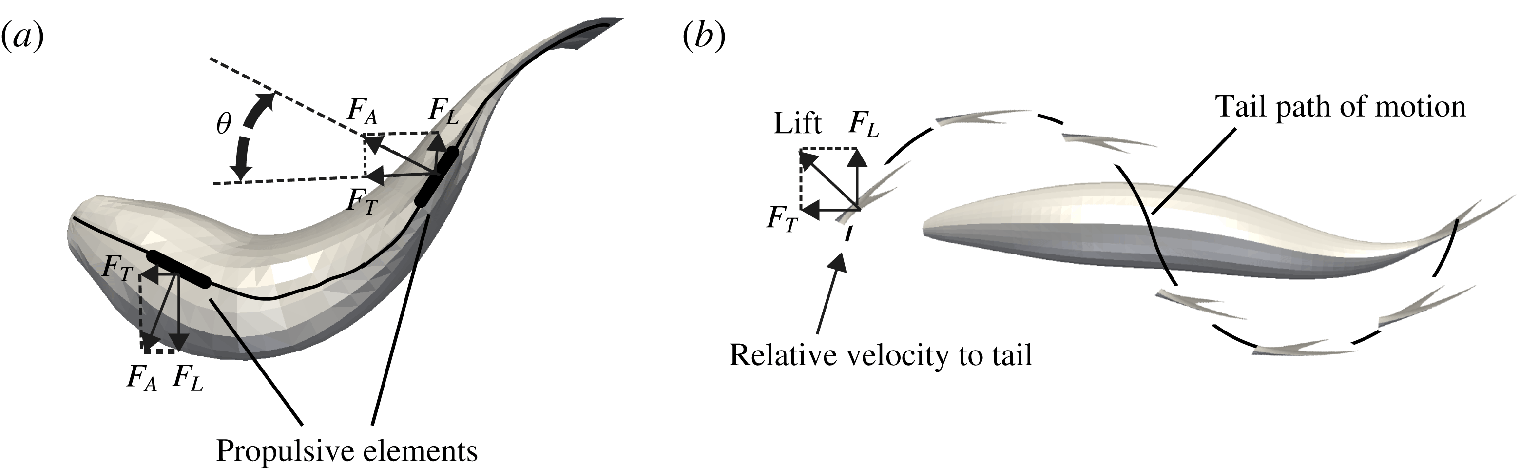
Aquatic swimming has fascinated scientists for more than a century, with the pioneering works of Breder (Reference Breder1926), Gray (Reference Gray1933) and Lighthill (Reference Lighthill1960) to explain how body motion leads to propulsion. There are two main thrust generation mechanisms employed by fish for steady propulsion using their body and caudal fin (figure 1): (1) the added-mass (reactive) mechanism; and (2) the lift-based (vorticity, circulatory) mechanism. In the added-mass mechanism, the propulsive movements of the fish’s body, which are in the form of backward-travelling waves, or their pectoral fins accelerate the adjacent fluid (Gray Reference Gray1933; Webb Reference Webb1984). The acceleration of adjacent fluid generates a reactive (added-mass) force perpendicular to each propulsive element, which has a component in the thrust direction as shown figure 1(a) (Gray Reference Gray1933; Webb Reference Webb1984). This mechanism is typically used by undulatory swimmers, such as eel, which have large undulations from head to tail and short wavelengths for the propulsive travelling wave (smaller than the fish length). In the lift-based (vorticity, circulatory) mechanism, the thrust is generated by the oscillations of the large tail (caudal fin) of the fish (Chopra Reference Chopra1976). The tail motion consists of heaving (moving side to side) and pitching (changing the angle of attack) during each tail beat cycle, as shown in figure 1(b). The flow circulation around the tail, which acts similar to an airfoil, generates a lift force on the tail. This lift force acts perpendicular to the moving direction of the flapper, in contrast to the added-mass force, which acts opposite to the acceleration direction of the undulating body (figure 1). At each instant the angle of the tail is such that the lift force has a component in the forward (thrust) direction (figure 1 b). Fish that use this mechanism, such as tuna, have fewer undulations of the body and more oscillations of the tail. Breder (Reference Breder1926) classified the swimming modes for body–caudal fin propulsion based on a continuum of propulsive movements from undulatory to oscillatory.
Rosenberger (Reference Rosenberger2001) also classified batoid fish based on a continuum of propulsive movements from undulatory to oscillatory (flapping). Batoid fish include a diverse variety of species such as the manta ray, stingray and sawfish with unique body forms and ways of swimming. Batoids usually have flattened bodies, extended pectoral fins and a calcified cartilage skeleton, and swim by some form of flapping, wing undulation or a combination of both (Rosenberger Reference Rosenberger2001). For instance, a freshwater stingray swims by passing a travelling wave across its pectoral disk (undulatory) (Blevins & Lauder Reference Blevins and Lauder2012), whereas a manta ray swims by flapping its wings (oscillatory) (Fish et al. Reference Fish, Haj-Hariri, Smits, Bart-Smith, Iwasaki and Bar-Cohen2012). Because of the combination of undulations and oscillations in batoids and their single, large propulsive fins, ray-like swimming is a good test case for investigating new propulsive mechanisms. Nevertheless, the lack of understanding of these alternative means of thrust production prohibits them from being fully utilized in bio-inspired designs (Fish et al. Reference Fish, Haj-Hariri, Smits, Bart-Smith, Iwasaki and Bar-Cohen2012). Understanding the underlying physics of different propulsion mechanisms can be achieved through well-controlled experiments and simulations.
Schematic of propulsion mechanisms in aquatic swimming. (a) Thrust generation by the added-mass (reactive) mechanism in which the propulsive elements accelerate the adjacent fluid backwards perpendicular to the elements, thereby creating a reaction force that has a component in the forward (thrust) direction. Adopted from Webb (Reference Webb1984). (b) Thrust generation by the lift-based (circulatory, vorticity) mechanism in which the tail/fin moves in such a way that the lift force created by the flow circulation (vorticity) around the tail/fin has a component in the forward (thrust) direction. Symbols:
 $F_{A}$
, added-mass force, which is normal to the propulsive element;
 $F_{T}$
, thrust force;
 $F_{L}$
, lateral force;
 ${\it\theta}$
, angle between propulsive element and swimming direction.

The added-mass mechanism, which is used by undulatory swimmers, has been investigated through analytical approaches (Lighthill Reference Lighthill1960; Wu Reference Wu1960, Reference Wu1971), numerical simulations (Liu & Kawachi Reference Liu and Kawachi1999; Kern & Koumoutsakos Reference Kern and Koumoutsakos2006; Borazjani & Sotiropoulos Reference Borazjani and Sotiropoulos2009; Alben et al.
Reference Alben, Witt, Baker, Anderson and Lauder2012) and experiments (Gray Reference Gray1933; Muller et al.
Reference Muller, Smit, Stamhuis and Videler2001; Tytell & Lauder Reference Tytell and Lauder2004; Clark & Smits Reference Clark and Smits2006). The early work using elongated-body theory has found relations for thrust, power and propulsive efficiency based on the wave speed of the propulsive wave on the body
 $V$
and the swimming speed
 $U$
(Lighthill Reference Lighthill1960). The propulsive wave that passes through the fish body accelerates the adjacent fluid (Gray Reference Gray1933), but in this theory the thrust of all propulsive elements cancel out through one tail beat cycle, except at the tail, i.e. the thrust is generated at the tail (Lighthill Reference Lighthill1960). Nevertheless, this method overestimates the thrust and drag by several-fold relative to estimates obtained based on drag coefficients for streamlined bodies at similar Reynolds numbers and fineness ratios (Lighthill Reference Lighthill1971). Clark & Smits (Reference Clark and Smits2006) built an elliptical undulatory robotic fin experimental apparatus and reported the thrust production and wake structure of the fin in cross-flow. In more recent studies, the hydrodynamics of this apparatus was explored (Dewey, Carriou & Smits Reference Dewey, Carriou and Smits2012), in which the wake structure and its relation to efficiency were discussed. They report that the swimming motion is more efficient when the leading- and trailing-edge vortices of subsequent cycles coalesce at the location where the streamwise fluid momentum is concentrated in the wake of the fin. It was shown that the Strouhal number (
 $St$
) can have large effects on the fin’s hydrodynamics. Clark & Smits (Reference Clark and Smits2006) report that the efficiency grows to a maximum as the Strouhal number approaches 0.25 and decreases steadily with Strouhal numbers greater than 0.25. Furthermore, at
 $St=0.15$
, the wake consists of a set of interconnected vortex tails; however, at
 $St=0.25$
, the wake structure changes to consist of twisted vortex structures. This shows that subtle differences in the Strouhal number can have a large impact on the accompanying hydrodynamics. Moored et al. (Reference Moored, Dewey, Smits and Haj-Hariri2012) found that, if the undulatory frequency of the fin matches the resonant frequency of the trailing-edge velocity profile, optimal propulsive efficiency occurs, similar to that found in Lewin & Haj-Hariri (Reference Lewin and Haj-Hariri2003).
The above experimental studies (Clark & Smits Reference Clark and Smits2006; Dewey et al. Reference Dewey, Carriou and Smits2012) utilize particle image velocimetry to visualize the associated flow fields on the midplane of the fin. However, to the best of our knowledge, there has been no investigation to date that has elucidated the three-dimensional (3D) flow over ray-like swimmers, and only one kinematic study with 3D data necessary for input into computational models. Here we present numerical simulations of a stingray whose body shape and kinematics are prescribed based on experimental measurement of 3D motion of the body and surface of the freshwater stingray during self-propelled swimming.
The lift-based mechanism, which is used by oscillatory swimmers, has been investigated both computationally and experimentally through heaving and pitching foils with simple geometries (Koochesfahani Reference Koochesfahani1989; Anderson, Streitlien & Barrett Reference Anderson, Streitlien and Barrett1998; Lewin & Haj-Hariri Reference Lewin and Haj-Hariri2003; Dong, Mittal & Najjar Reference Dong, Mittal and Najjar2006) – see the review by Triantafyllou, Techet & Hover (Reference Triantafyllou, Techet and Hover2004) – and fish-like swimmers (Wolfgang et al. Reference Wolfgang, Anderson, Grosenbaugh, Yue and Triantafyllou1999; Nauen & Lauder Reference Nauen and Lauder2001; Zhu et al. Reference Zhu, Wolfgang, Yue and Triantafyllou2002; Borazjani & Sotiropoulos Reference Borazjani and Sotiropoulos2008) – see the review by Fish & Lauder (Reference Fish and Lauder2006). The flapping two-dimensional (2D) foil experiments of Anderson et al. (Reference Anderson, Streitlien and Barrett1998) have indicated that high efficiency is associated with the formation of a moderately strong leading-edge vortex (LEV) on alternating sides of the foil per half-cycle, which is convected downstream and interacts with trailing-edge vorticity, resulting eventually in the formation of a reverse Kármán street. The simulations of Dong et al. (Reference Dong, Mittal and Najjar2006) for low-aspect-ratio foils have also shown the shedding of the LEVs similar to the experiments. Lewin & Haj-Hariri (Reference Lewin and Haj-Hariri2003) also showed that the foil efficiency reduces when the LEV gets separated. Simulations of straight-line swimming of a Danio by Wolfgang et al. (Reference Wolfgang, Anderson, Grosenbaugh, Yue and Triantafyllou1999) and Zhu et al. (Reference Zhu, Wolfgang, Yue and Triantafyllou2002) also indicated that the constructive interaction of the vorticity shed by the body and the wake results in efficient propulsion.
Borazjani & Sotiropoulos (Reference Borazjani and Sotiropoulos2008, Reference Borazjani and Sotiropoulos2009, Reference Borazjani and Sotiropoulos2010) investigated different modes of steady swimming, defined consistent thrust and efficiency measures that do not depend on a reference pressure, and found that the large-scale features of the wake structure are dependent on Strouhal number and that the efficiency–Reynolds number relation depends on the type of swimming. In mackerel-like swimming with lift-based thrust generation, the efficiency is maximized in the inertial flow regime (high Reynolds number); whereas in eel-like swimming with added-mass (reactive) thrust generation, the efficiency is maximized in the transitional flow regime (intermediate Reynolds number
 $Re\approx 4000$
) (Borazjani & Sotiropoulos Reference Borazjani and Sotiropoulos2010). Furthermore, kinematics has a larger effect than body shape on these trends (Borazjani & Sotiropoulos Reference Borazjani and Sotiropoulos2010). These simulations also showed that there are more fluctuations in the thrust generated by the lift-based mechanism than by the added-mass mechanism (Borazjani Reference Borazjani2015). Fast-start escape behaviours of different fish species have also been investigated numerically (Borazjani et al.
Reference Borazjani, Sotiropoulos, Tytell and Lauder2012; Borazjani Reference Borazjani2013b
).
The focus of most previous numerical and experimental studies has been on the trailing wake generated by the fins. In fact, there is no investigation that reports LEV formation, which is one of the most important force enhancement features for the lift-based mechanism in insects, birds and bats (Ellington et al. Reference Ellington, Van Den Berg, Willmott and Thomas1996; Van Den Berg & Ellington Reference Van Den Berg and Ellington1997; Birch & Dickinson Reference Birch and Dickinson2001; Sane Reference Sane2003; Videler, Stamhuis & Povel Reference Videler, Stamhuis and Povel2004; Muijres et al. Reference Muijres, Johansson, Barfield, Wolf, Spedding and Hedenström2008; Lentink & Dickinson Reference Lentink and Dickinson2009b ; Chang et al. Reference Chang, Ting, Su, Soong and Yang2013; Thielicke & Stamhuis Reference Thielicke and Stamhuis2015). Borazjani & Daghooghi (Reference Borazjani and Daghooghi2013) reported for the first time the LEV reattachment on the fish’s tail, enhancing the thrust generation by the tail, in the inertial flow regime at Strouhal numbers commonly seen in fish swimming. LEV reattachment happens when the angle of attack of the foil increases until the flow separates at the leading edge. The flow reattaches at the trailing edge of the foil, thus maintaining the Kutta condition (Kuethe & Schetzer Reference Kuethe and Schetzer1950). This separation on the leading edge creates a strong suction pressure, increasing thrust and lift (Earnshaw Reference Earnshaw1962). From another viewpoint, the additional vorticity in the LEV increases the circulation around the wing/foil, and thus increases the lift (Ellington et al. Reference Ellington, Van Den Berg, Willmott and Thomas1996). The LEV has been estimated to increase the lift by as much as 40 % during slow flight of bats by showing that the ratio of the circulation of the leading to the trailing vortex is around 40 % (Muijres et al. Reference Muijres, Johansson, Barfield, Wolf, Spedding and Hedenström2008). Borazjani & Daghooghi (Reference Borazjani and Daghooghi2013) reported that the delta shape is not required to produce a stable LEV on the tail by showing the reattachment of the flow and the LEV on a rectangular tail (no swept-back angle). We also report LEV formation on the disk-shaped stingray wings here and show that the LEV generates a low-pressure region that enhances thrust generation in these rays.
LEV dynamics have been widely studied, and the LEV often grows and starts shedding for translating 2D foils (Dickinson & Gotz Reference Dickinson and Gotz1993; Wang Reference Wang2000; Kim & Gharib Reference Kim and Gharib2010; Beem, Rival & Triantafyllou Reference Beem, Rival and Triantafyllou2012; Pitt Ford & Babinsky Reference Pitt Ford and Babinsky2013) or 2D flapping foils (Anderson et al.
Reference Anderson, Streitlien and Barrett1998; Dong et al.
Reference Dong, Mittal and Najjar2006), but it remains stable/attached for 3D rotating blades (Ellington et al.
Reference Ellington, Van Den Berg, Willmott and Thomas1996; Van Den Berg & Ellington Reference Van Den Berg and Ellington1997; Aono, Liang & Liu Reference Aono, Liang and Liu2008; Lentink & Dickinson Reference Lentink and Dickinson2009b
; Ozen & Rockwell Reference Ozen and Rockwell2012; Harbig, Sheridan & Thompson Reference Harbig, Sheridan and Thompson2013; Cheng et al.
Reference Cheng, Roll, Liu, Troolin and Deng2014). A spanwise flow that causes the LEV spiral towards the tip (Maxworthy Reference Maxworthy1981; Ellington et al.
Reference Ellington, Van Den Berg, Willmott and Thomas1996; Van Den Berg & Ellington Reference Van Den Berg and Ellington1997; Wang Reference Wang2005; Lentink & Dickinson Reference Lentink and Dickinson2009b
) and recently vorticity annihilation (Wojcik & Buchholz Reference Wojcik and Buchholz2014) is suggested as a stabilizing mechanism by providing a sink of vorticity to balance the vorticity flux of the leading-edge shear layer. Spanwise flow magnitude was found to be related to the Reynolds number (
 $Re$
) (Aono et al.
Reference Aono, Liang and Liu2008). Spanwise flow was not observed at low
 $Re$
(Birch & Dickinson Reference Birch and Dickinson2001), but existed at higher
 $Re$
(Birch, Dickson & Dickinson Reference Birch, Dickson and Dickinson2004). Wojcik & Buchholz (Reference Wojcik and Buchholz2014) observed that an opposite-sign vorticity layer is extracted by the LEV, and suggested that vorticity annihilation due to interaction between them might be an important mechanism for LEV stabilization. The secondary vortex has been observed on delta wings as well (Gad-el Hak & Blackwelder Reference Gad-el Hak and Blackwelder1985). Lentink & Dickinson (Reference Lentink and Dickinson2009a
,Reference Lentink and Dickinson
b
) suggest rotational acceleration, which scales with Rossby number (
 $Ro$
), as the stabilizing mechanism on insect wings. They state that the condition for stability of the LEV is
 $Ro$
of order one, and at high
 $Ro$
(e.g. translating wings) LEV becomes unstable (Lentink & Dickinson Reference Lentink and Dickinson2009b
). Nevertheless, the stability mechanism of the LEV in insect flight and aquatic swimming might be different, and the dynamics of the LEV on the surface of freely swimming fish remains poorly studied.
The effect of fin/wing deformations of a flexible structure on the LEV is not fully understood either. The fin/wing deformations can be generated actively, e.g. by muscles, actuators, etc., or passively, e.g. by deformation of a flexible structure due to fluid forces. Pederzani & Haj-Hariri (Reference Pederzani and Haj-Hariri2006) analysed the effects chordwise flexibility on a vertically oscillating foil, and compared it against rigid foils. Pederzani & Haj-Hariri (Reference Pederzani and Haj-Hariri2006) found that flexible foils are more efficient than rigid ones, and also produce more thrust because of snapping, which sheds vortices with increased strength, thus increasing thrust. Simulations of a flexible wing have shown that wing deformations might be responsible for stabilizing the LEV, and hence augmenting the aerodynamic force generation relative to a rigid wing (Nakata & Liu Reference Nakata and Liu2012). In another study for low to medium angles of attack, in contrast, as flexibility of the wing was increased, its ability to generate aerodynamic forces was decreased monotonically (Zhao et al. Reference Zhao, Huang, Deng and Sane2010). The flexibility at high angles of attack might not have the same effect and can slightly increase the forces (Du & Sun Reference Du and Sun2010). The flexibility of bumblebee wings also increases their lift generation (Mountcastle & Combes Reference Mountcastle and Combes2013). More recently, it was shown that the forces are maximized at the first and second structural resonant frequencies of the wing (Eberle, Reinhall & Daniel Reference Eberle, Reinhall and Daniel2014). Quinn, Lauder & Smits (Reference Quinn, Lauder and Smits2014) also report a localized boost to net thrust near resonant frequencies for flexible plates. Note that, in the above studies, the deformation of the fin/wing was passive, whereas in our simulations of the stingray the deformation of the wing is prescribed from experiments, i.e. active deformations.
The work presented here investigates the hydrodynamics of stingray locomotion using self-propelled simulations similar to our previous works (Borazjani & Sotiropoulos Reference Borazjani and Sotiropoulos2010; Borazjani & Daghooghi Reference Borazjani and Daghooghi2013) using the sharp-interface immersed boundary method (Ge & Sotiropoulos Reference Ge and Sotiropoulos2007; Borazjani, Ge & Sotiropoulos Reference Borazjani, Ge and Sotiropoulos2008; Borazjani et al. Reference Borazjani, Ge, Le and Sotiropoulos2013) (§ 2). Stingray geometry is modelled accurately from laser-scan data of a freshwater stingray (§ 2.1). Stingray body motion is prescribed based on experimental measurements in which the 3D movement of 31 points on the dorsal stingray surface is measured through time at two swimming speeds (Blevins & Lauder Reference Blevins and Lauder2012). The body motion is prescribed (§ 2.2), but the motion of the centre of mass is calculated through a fluid–structure interaction coupling (Borazjani et al. Reference Borazjani, Ge and Sotiropoulos2008). The simulations are continued until the stingray reaches quasi-steady state, i.e. the average swimming velocity is constant, at which the swimming performance and the 3D wake is analysed (§ 3). Finally, the results are discussed in § 4.
2. Materials and methods
2.1. Measurements of the stingray body motion and geometry
Five sets of experimental data are used in this work based on the 3D body motion measurements of a freshwater stingray, P. orbignyi (Blevins & Lauder Reference Blevins and Lauder2012). Blevins & Lauder (Reference Blevins and Lauder2012) carried out their experiments at two different swimming speeds: a fast speed of
 $U=2.5L~\text{s}^{-1}$
(
 $L$
is the disk length of the ray) and a slow speed of
 $U=1.5L~\text{s}^{-1}$
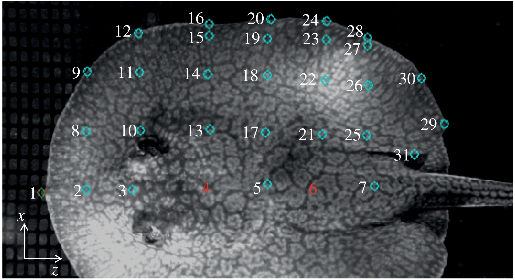
. Three of the sets of experimental data are from experiments at the fast speed, while two are from stingrays swimming at the slower speed. These experimental data provide 3D coordinate positions of 31 nodes scattered in a grid-like manner across the stingray’s pectoral disk over approximately one swimming cycle, as shown in figure 2 (Blevins & Lauder Reference Blevins and Lauder2012). For details on the experiments, the rays and data collection methods, see Blevins & Lauder (Reference Blevins and Lauder2012). These measurements are analysed here to create a semi-analytical model of the stingray motion as described in the following section.
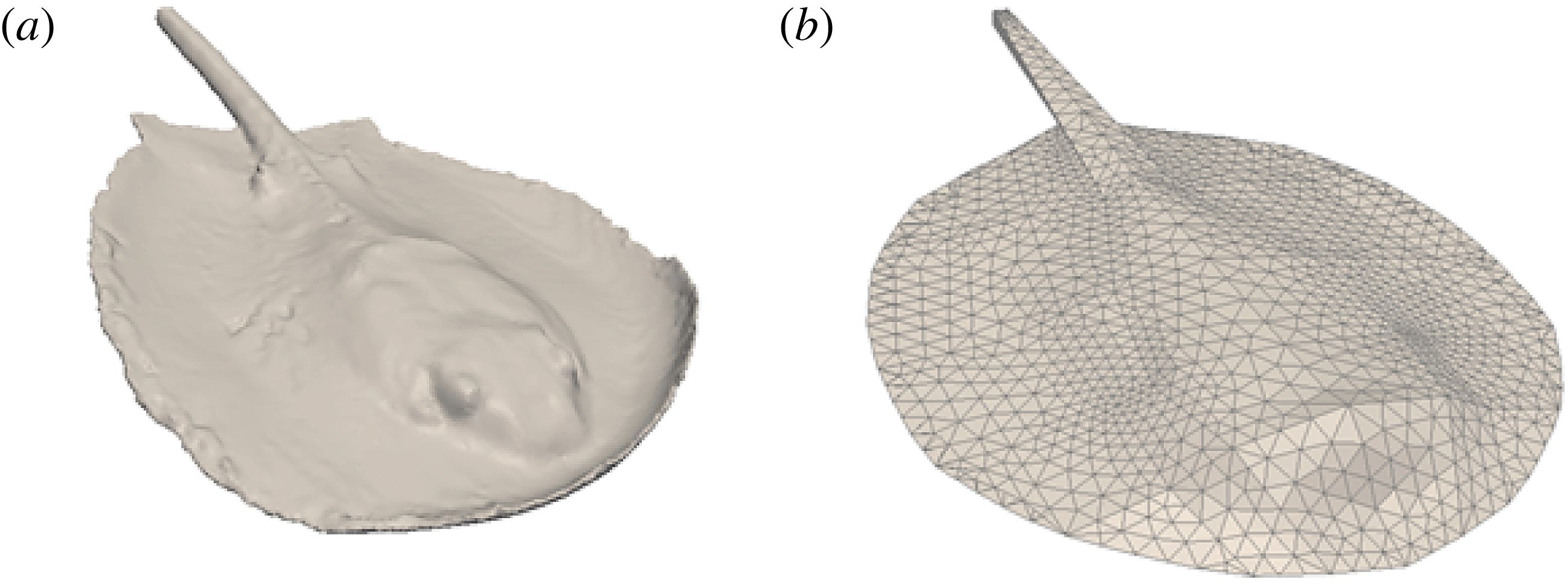
The body of a stingray was scanned using a 3D laser scanner to obtain the body geometry of a stingray (figure 3 a). The laser-scan geometry was smoothed and asymmetry in the laser scanner geometry, created by asymmetric folding of the stingray wings during the scan, was removed for the simulations. Furthermore, the stingray’s pelvic fins were removed from the geometry because they are tucked underneath the ray’s caudal region during swimming and thus have minimal effect on the hydrodynamics of locomotion. The smoothed stingray surface was meshed with triangular elements for use in our simulations (figure 3 b).
Measurement of 3D coordinate positions of 31 points on the stingray’s body and pectoral fin during free swimming at two speeds. See Blevins & Lauder (Reference Blevins and Lauder2012) for details. Note that the
 $y$
direction is directed out of the page.

Geometry of the stingray’s body and pectoral fin. (a) Stingray shape from the original laser-scan data, in which the asymmetries and curling of the fins due to the body position when this animal was preserved are evident. (b) The smoothed stingray after removing the asymmetries and meshing the surface with triangular elements.

2.2. Stingray body motion analysis
Body and pectoral undulations are measured for 31 points on the stingray (figure 2). The motion of the other locations on the stingray body needs to be determined from these measurements. Fourier series are used to create a kinematic description of the swimming motion of the stingray because of the wave-like nature of the undulations. The Fourier method used here can be considered as a 2D extension of the method employed by Videler & Hess (Reference Videler and Hess1984) for saithe and mackerel. Because an infinite number of terms can be used in the Fourier series, the number of terms that adequately capture the motion of the experimental data must be discovered. To uncover how many terms adequately capture the swimming motion, the
 $y$
component of the experimental data (highest undulation direction) was curve-fitted with a Fourier series using a nonlinear least-squares approximation similar to Videler & Hess (Reference Videler and Hess1984):
 $$\begin{eqnarray}\displaystyle y(t)=a_{0}+\mathop{\sum }_{q=0}^{N}a_{q}\sin (q{\it\omega}t)+b_{q}\cos (q{\it\omega}t), & & \displaystyle\end{eqnarray}$$
where
 $a_{q}$
and
 $b_{q}$
are the Fourier coefficients,
 ${\it\omega}$
is the natural frequency,
 $t$
is time and
 $N$
is the total number of Fourier terms. The Fourier series is reformulated into a travelling wave as follows:
 $$\begin{eqnarray}\displaystyle y(t)=\mathop{\sum }_{q=0}^{N}h_{q}\cos (q{\it\omega}(t-{\it\phi}_{q})), & & \displaystyle\end{eqnarray}$$
where
 $h_{q}=\sqrt{a_{q}^{2}+b_{q}^{2}}$
and
 ${\it\phi}_{q}=(1/q{\it\omega})\tan ^{-1}(b_{q}/a_{q})$
. The first three Fourier coefficients
 $a_{q}$
and
 $b_{q}$
were obtained by the nonlinear least-squares curve-fitting, and the Fourier coefficient
 $h_{q}$
and phase angle
 ${\it\phi}_{q}$
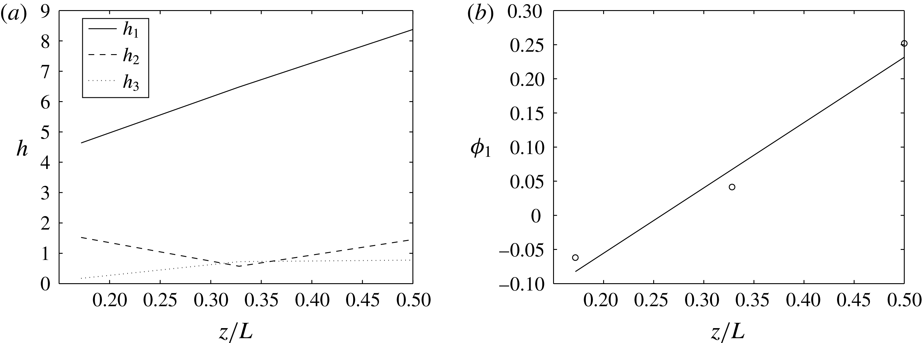
were calculated for the experimental nodes in the distal–medial to distal–posterior region of the pectoral disk, as they have the most prominent undulations. It was found that the first Fourier coefficient
 $h_{1}$
is dominant in all cases. Furthermore, the phase angle
 ${\it\phi}_{1}$
varies almost linearly with the position
 $z$
along the ray body from head to tail, i.e.
 ${\it\tau}_{1}=Cz$
(
 $C$
is a constant), as shown in figure 4 for nodes 15, 19 and 23 that lie on the same row (
 $x$
position) on the stingray wing – see figure 2. Analysis in the lateral direction showed similar results but with a frequency double that in the
 $y$
direction. Note that there are no undulations in the axial (swimming) direction
 $z$
. Therefore, we can use the first Fourier mode as a good approximation for the motion of the stingray as follows:
 $$\begin{eqnarray}\displaystyle & x(t)=A_{x}(y,z)\cos (kz-4{\rm\pi}ft), & \displaystyle\end{eqnarray}$$
 $$\begin{eqnarray}\displaystyle & y(t)=A_{y}(y,z)\cos (kz-2{\rm\pi}ft), & \displaystyle\end{eqnarray}$$
 $$\begin{eqnarray}\displaystyle & z(t)=z(0), & \displaystyle\end{eqnarray}$$
where
 $k$
is the wavenumber,
 $f$
is the frequency of the undulatory motion, and
 $A_{x}$
and
 $A_{y}$
are the amplitudes of the motion in the vertical and lateral directions. In what follows we describe how these constants are obtained from the five experimental datasets.
Fourier analysis of the body motion: (a) the first three Fourier coefficients and (b) the phase angle
 ${\it\phi}_{1}$
for marker points 15, 19 and 23 on the body. The first Fourier coefficient
 $h_{1}$
is dominant and the phase angle varies linearly to a good approximation along the axial (
 $z$
) direction.

The frequency
 $f$
is obtained from the period of the undulations of the experimental data. Because of noise in the experimental measurements, the measured positions are first smoothed using a moving-average method, and the period for each experimental node is obtained from the smoothed measured positions. The frequency for each dataset is obtained by averaging the frequencies of all the experimental nodes after eliminating the outliers. The frequency for the slow and fast cases is obtained by averaging the frequencies of the relevant two and three datasets, respectively. The frequency is found to be
 $f=2.385\pm 0.276$
and
 $3.384\pm 0.517~\text{Hz}$
for slow and fast swimming, respectively.
The wavenumber
 $k=2{\rm\pi}/{\it\lambda}$
(
 ${\it\lambda}$
is the wavelength) of the ray’s body wave, travelling backwards in the swimming (
 $z$
) direction, is obtained by calculating the wave speed
 $V$
from the vertical (
 $y$
) component of the experimental data, i.e.
 $k=2{\rm\pi}f/V$
. The wave speed is obtained by determining the speed at which the peak of the travelling wave progresses across the fish. The wave speed for the experimental nodes is obtained and averaged to find the average wave speed for each dataset. The wave speeds for the two slow and the three fast swimming datasets are averaged to find the wave speed for the slow and fast cases, respectively. The wave speed is found to be
 $V=253.568\pm 48.518$
and
 $359.482\pm 85.656~\text{mm}~\text{s}^{-1}$
for slow and fast cases, respectively. The wavenumber non-dimensionalized by
 $L$
is, therefore,
 $k=7.565\pm 4.572$
and
 $7.571\pm 4.851$
for slow and fast cases, respectively. It can be observed that the nominal wavenumber is basically the same in both slow and fast cases considering its large deviations, i.e. the wavenumber (wavelength) does not change between fast and slow cases – see Blevins & Lauder (Reference Blevins and Lauder2012) for more details.
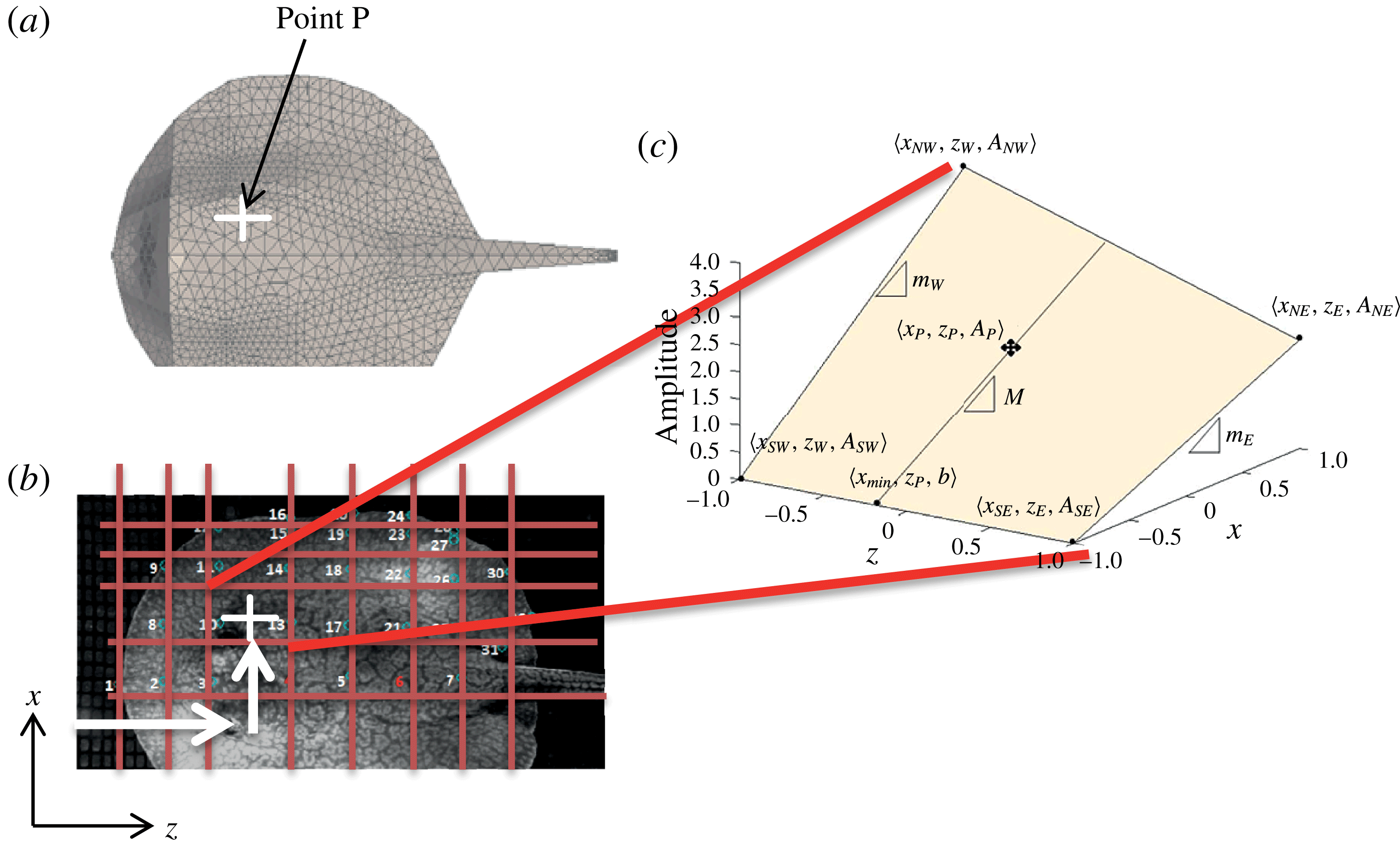
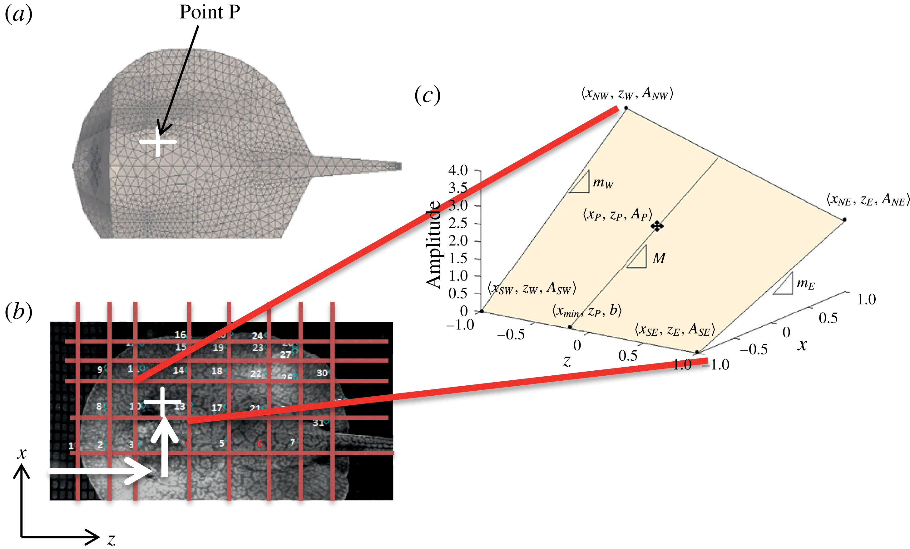
The amplitude for a given point P is obtained by bilinear interpolation from the amplitude of the four surrounding experimental nodes (figure 5). Owing to the grid-like structure of the experimental nodes, we can find the four surrounding nodes by comparing the axial (
 $z$
) and lateral (
 $x$
) location of point P with the experimental points at time zero, i.e. initial stretched state (figure 5
b). The surrounding nodes will not change at later times in the cycle. The amplitudes
 $A_{x}$
and
 $A_{y}$
at all experimental nodes are set to the average of the amplitudes of the same node in the five datasets, because the amplitudes did not change significantly with the swimming speed, i.e. they were similar in fast and slow cases. The amplitudes in the vertical direction
 $A_{y}$
were typically several-fold larger than the amplitudes in the lateral direction
 $A_{x}$
.
Schematic representation of bilinear interpolation of movement amplitudes: (a) point P on the surface of the stingray for which the amplitudes need to be obtained; (b) the four experimental nodes around point P are found; and (c) the amplitudes at point P are reconstructed by bilinear interpolation from the amplitudes at the surrounding experimental nodes.
2.3. The governing equations and the numerical method
To simulate stingray locomotion, we use the curvilinear immersed boundary (CURVIB) method (Ge & Sotiropoulos Reference Ge and Sotiropoulos2007; Borazjani et al. Reference Borazjani, Ge and Sotiropoulos2008) with prescribed body motion (relative to the centre of mass) from experimental measurements (as described in the previous sections), and calculated the motion of the centre of mass based on the net fluid forces, i.e. self-propelled simulations (Borazjani & Sotiropoulos Reference Borazjani and Sotiropoulos2010; Borazjani & Daghooghi Reference Borazjani and Daghooghi2013), under realistic Reynolds numbers using large-eddy simulations (LES). The governing equation for the motion of the stingray’s centre of mass is Newton’s second law:
 $$\begin{eqnarray}\displaystyle M_{red}\frac{\text{d}\boldsymbol{U}^{\ast }}{\text{d}t}=\boldsymbol{F}^{\ast }. & & \displaystyle\end{eqnarray}$$
Here
 $M_{red}=m/({\it\rho}L^{3})$
is the reduced mass (
 $m$
is the mass of the swimmer and
 ${\it\rho}$
is the density of the fluid), which is set at 14.5 in this work;
 $\boldsymbol{F}^{\ast }=\boldsymbol{F}/({\it\rho}U^{2}L^{2})$
is the force coefficient acting on the swimmer (
 $U$
is the swimming speed of the ray from experiments); and
 $\boldsymbol{U}^{\ast }$
is the swimming speed of the swimmer non-dimensionalized by
 $U$
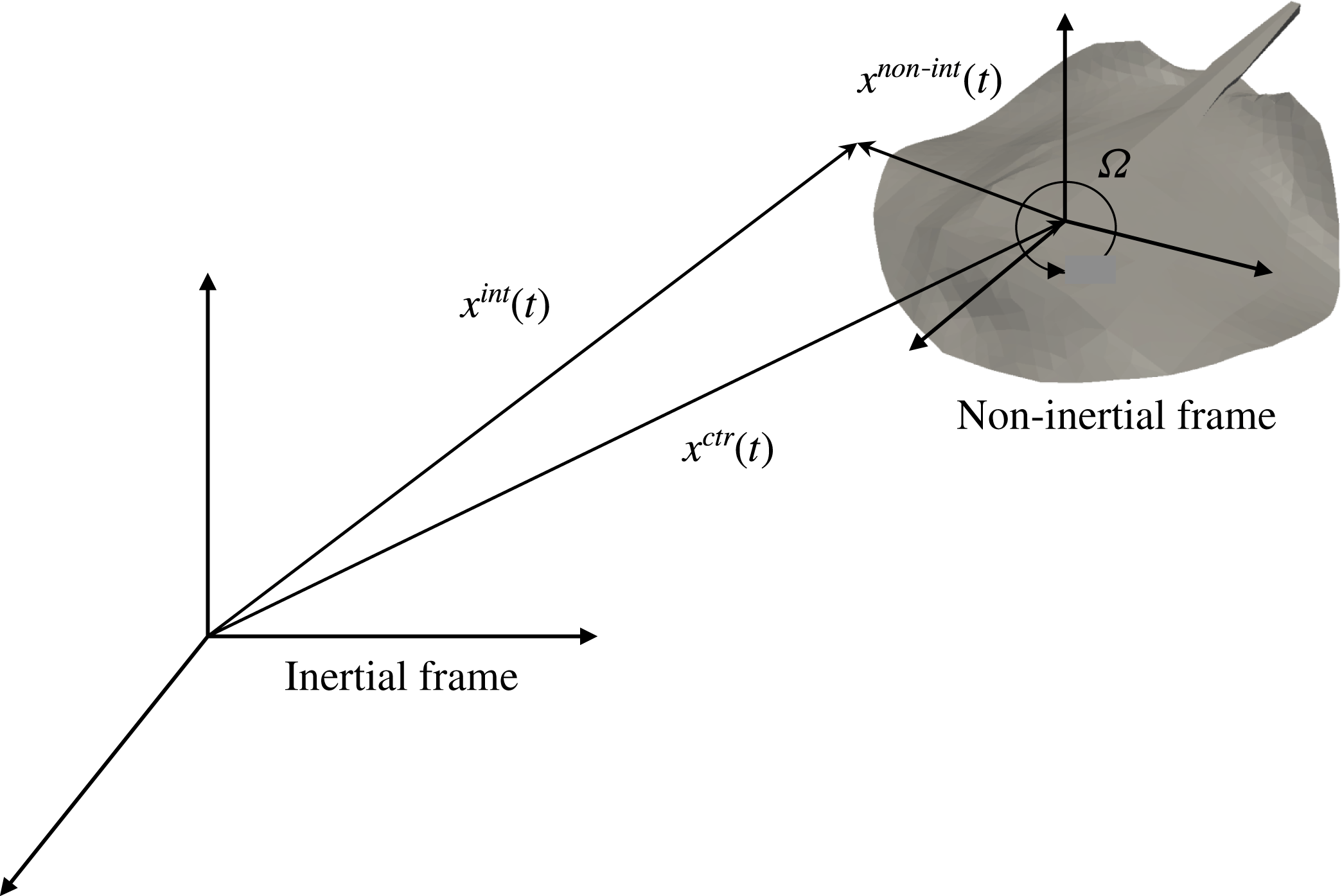
. The system is restricted in the rotational directions to avoid roll, pitch and yaw. Because the coordinate frame is attached to the centre of mass of the swimmer, this is the velocity of the coordinate system as well (figure 6). This equation is coupled with the fluid equations of motion using our strongly coupled partitioned approach (Borazjani et al.
Reference Borazjani, Ge and Sotiropoulos2008) similar to our previous self-propelled simulations (Borazjani & Sotiropoulos Reference Borazjani and Sotiropoulos2010; Borazjani & Daghooghi Reference Borazjani and Daghooghi2013).
Schematic of the inertial and non-inertial reference frames. The non-inertial frame is attached to the centre of mass of the stingray and moves with it;
 $x^{non\text{-}int}$
and
 $x^{int}$
are position vectors in the non-inertial and inertial reference frames, respectively; the origin of the non-inertial reference frame is positioned at
 $x^{ctr}$
from the inertial reference frame; and
 ${\it\Omega}$
is the instantaneous angular velocity of the non-inertial frame.

The governing equations for the fluid flow are the incompressible Navier–Stokes equations in a general non-inertial frame of reference (attached to the centre of mass of the self-propelled stingray – see figure 6) in curvilinear coordinates (
 ${\it\xi}^{r}={\it\xi}^{r}(x_{1},x_{2},x_{3})$
to easily handle curvilinear or stretched grids) and filtered for LES, which in tensor notation (repeated indices imply summation) read as follows (
 $q,r,s,m=1,2,3$
):
 $$\begin{eqnarray}\displaystyle & \displaystyle J\frac{\partial U^{r}}{\partial {\it\xi}^{r}}=0, & \displaystyle\end{eqnarray}$$
 $$\begin{eqnarray}\displaystyle \displaystyle \frac{\partial U^{r}}{\partial t} & = & \displaystyle {\it\xi}_{q}^{r}\left(-\frac{\partial }{\partial {\it\xi}^{s}}((U^{s}-V^{s})u_{q}-U^{s}w_{q})-\frac{\partial }{\partial {\it\xi}^{s}}\left(\frac{{\it\xi}_{q}^{s}}{J}\frac{p}{{\it\rho}}\right)\right.\nonumber\\ \displaystyle & & \displaystyle \left.+\,\frac{\partial }{\partial {\it\xi}^{s}}\left({\it\nu}\frac{g^{sm}}{J}\frac{\partial u_{q}}{\partial {\it\xi}^{m}}\right)-\frac{{\it\xi}_{m}^{s}}{{\it\rho}J}\frac{\partial {\it\tau}_{qm}}{\partial {\it\xi}^{s}}\right).\end{eqnarray}$$
Here
 $J=|\partial ({\it\xi}^{1},{\it\xi}^{2},{\it\xi}^{3})/\partial (x_{1},x_{2},x_{3})|$
is the determinant of the Jacobian of the transformation,
 ${\it\xi}_{q}^{r}=\partial {\it\xi}^{r}/\partial x_{q}$
;
 $g^{rm}$
is the contravariant metric of the transformation,
 $g^{rm}={\it\xi}_{q}^{r}{\it\xi}_{q}^{m}$
;
 $p$
is the filtered pressure;
 ${\it\rho}$
is the density;
 ${\it\nu}$
is the kinematic viscosity;
 $U^{r}=u_{m}{\it\xi}_{m}^{r}/J$
and
 $V^{r}=v_{m}{\it\xi}_{m}^{r}/J$
are the filtered contravariant velocities for the fluid and the grid, respectively; and
 $u_{q}$
,
 $v_{q}$
and
 $w_{q}$
are the filtered Cartesian velocities defined as follows (Beddhu, Taylor & Whitfield Reference Beddhu, Taylor and Whitfield1996; Kim & Choi Reference Kim and Choi2006; Borazjani et al.
Reference Borazjani, Ge, Le and Sotiropoulos2013):
 $$\begin{eqnarray}\displaystyle & u_{q}=u_{q}^{non\text{-}int}+v_{q}=\unicode[STIX]{x1D618}_{qr}u_{r}^{int}, & \displaystyle\end{eqnarray}$$
 $$\begin{eqnarray}\displaystyle & v_{q}=w_{q}+u_{q}^{ctr}, & \displaystyle\end{eqnarray}$$
 $$\begin{eqnarray}\displaystyle & w_{q}={\it\epsilon}_{qlm}{\it\Omega}_{l}x_{m}^{int}, & \displaystyle\end{eqnarray}$$
where
 $u_{q}^{ctr}=u_{q}^{ctr}(t)$
and
 ${\it\Omega}_{q}={\it\Omega}_{q}(t)$
are the translational and rotational velocity of the non-inertial frame, respectively, relative to the inertial frame; and
 $u_{q}^{non\text{-}int}=u_{q}^{non\text{-}int}(x_{r},t)$
and
 $u_{q}^{int}=u_{q}^{int}(x_{r}^{int},t)$
are the Cartesian components of the filtered velocity vector as observed by a viewer in the non-inertial and inertial frames, respectively. Note that
 $u_{q}=u_{q}(x_{r},t)$
is not equal to the absolute (inertial) velocity (
 $u_{q}^{int}$
) if the non-inertial frame is rotating. In fact, it has the same magnitude but has been rotated similar to the rotation of the non-inertial frame relative to the inertial frame. One can consider
 $v_{q}=v_{q}(x_{r},t)$
as the components of the grid velocity vector due to the motion of the non-inertial reference frame, while
 $w_{q}=w_{q}(x_{r},t)$
are the components of the grid velocity vector due to the rotation of the non-inertial reference frame, and
 ${\it\epsilon}_{qlm}$
is the alternating tensor indicating the cross-product of the vectors
 ${\it\bf\Omega}(t)$
and
 $\boldsymbol{x}^{int}(t)$
. Finally,
 $\unicode[STIX]{x1D618}_{qr}$
is the orthogonal rotation tensor that rotates the non-inertial frame to the inertial frame orientation, i.e.
 $x_{q}=x_{q}^{non\text{-}int}=\unicode[STIX]{x1D618}_{qr}(x_{r}^{int}-x_{r}^{ctr})$
(
 $q,r=1$
to 3) (see figure 6);
 $x_{q}=x_{q}^{non\text{-}int}=x_{q}(t)$
and
 $x_{q}^{int}=x_{q}^{int}(t)$
are the components of the position vectors in the non-inertial and inertial reference frames, respectively; and the origin of the non-inertial reference frame is positioned at
 $\boldsymbol{x}^{ctr}=\boldsymbol{x}^{ctr}(t)$
from the inertial reference frame (see figure 6). The equations in the inertial reference frame can easily be recovered by setting the translational and angular velocities of the non-inertial frame to zero.
The
 ${\it\tau}_{qm}$
in (2.8) is the subgrid stress (SGS) tensor for LES. The SGS terms are modelled using the Smagorinsky model (Smagorinsky Reference Smagorinsky1963)
 ${\it\tau}_{qm}-({\it\tau}_{rr}{\it\delta}_{qm})/3=-2{\it\mu}_{t}\overline{\unicode[STIX]{x1D61A}}_{qm}$
, where the overline denotes the grid filtering operation, and
 $\overline{\unicode[STIX]{x1D61A}}_{qm}$
is the filtered strain-rate tensor. The eddy viscosity is given by
 ${\it\mu}_{t}={\it\rho}C_{S}{\it\Delta}^{2}|\overline{\unicode[STIX]{x1D61A}}|$
, where
 $C_{S}$
is the Smagorinsky constant,
 ${\it\Delta}$
is the filter size, and
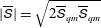 $|\overline{\unicode[STIX]{x1D61A}}|=\sqrt{2\overline{\unicode[STIX]{x1D61A}}_{qm}\overline{\unicode[STIX]{x1D61A}}_{qm}}$
. The filter size is taken as the cube root of the cell volume. The Smagorinsky constant (
 $C_{S}$
) is computed using the dynamic Smagorinsky model (Germano et al.
Reference Germano, Piomelli, Moin and Cabot1991) implemented and applied in the context of our immersed boundary method (Kang et al.
Reference Kang, Borazjani, Colby and Sotiropoulos2012; Borazjani & Daghooghi Reference Borazjani and Daghooghi2013; Daghooghi & Borazjani Reference Daghooghi and Borazjani2015).
Equations (2.8) are solved over curvilinear grids using a fully staggered discretization with central schemes for the convective and viscous terms. The equations are integrated in time using an efficient second-order-accurate fractional-step methodology with a Jacobian-free Newton–Krylov solver for the momentum equations, and a GMRES solver enhanced with multigrid as a preconditioner for the Poisson equation (Ge & Sotiropoulos Reference Ge and Sotiropoulos2007; Borazjani et al. Reference Borazjani, Ge and Sotiropoulos2008). The code is parallelized using MPI and the parallel libraries of PETSc (Balay et al. Reference Balay, Buschelman, Gropp, Kaushik, Knepley, McInnes, Smith and Zhang2004) to efficiently utilize the supercomputing facilities available to the authors.
To handle the moving boundaries (body motion of the stingray), a sharp-interface immersed boundary method is used (Gilmanov & Sotiropoulos Reference Gilmanov and Sotiropoulos2005; Ge & Sotiropoulos Reference Ge and Sotiropoulos2007; Borazjani et al. Reference Borazjani, Ge and Sotiropoulos2008; Borazjani Reference Borazjani2013a ). In this method, the fluid grid is fixed and does not move with the boundary, which is more suitable for large deformations because it does not create highly skewed grids (Mittal & Iaccarino Reference Mittal and Iaccarino2005). The original immersed boundary, pioneered by Peskin (Peskin Reference Peskin1972, Reference Peskin1977; Peskin & McQueen Reference Peskin and McQueen1989), smeared the effect of boundaries over several grid nodes, which required additional resolution near the boundary. Since then, a number of sharp-interface methods have been developed (Mittal & Iaccarino Reference Mittal and Iaccarino2005). Here, the sharp interface is maintained by reconstructing the boundary conditions at the nodes that are exterior to, but adjacent to, the immersed boundary surface using wall functions along the local normal to the boundary (Khosronejad et al. Reference Khosronejad, Kang, Borazjani and Sotiropoulos2011; Kang et al. Reference Kang, Borazjani, Colby and Sotiropoulos2012):
 $$\begin{eqnarray}\displaystyle \frac{u}{u^{\ast }}=\left\{\begin{array}{@{}ll@{}}y^{+} & \text{if }y^{+}\leqslant y_{0}^{+},\\ {\displaystyle \frac{1}{{\it\kappa}}}\ln y^{+} & \text{if }y^{+}>y_{0}^{+},\end{array}\right. & & \displaystyle\end{eqnarray}$$
where
 $y^{+}=y/u{\it\nu}$
is the non-dimensional distance from the wall,
 $u$
is the velocity magnitude at the nearest node to the wall,
 $y$
is the distance off the wall,
 $u^{\ast }$
is the shear velocity,
 ${\it\kappa}$
is the von Kármán constant,
 ${\it\nu}$
is the kinematic viscosity, and
 $y_{o}^{+}$
is chosen to be 11.53 because the departure from the linear relation is significant (
 ${>}$
25 %) for
 $y^{+}>12$
(Pope Reference Pope2000). The immersed boundary surface is discretized using triangular elements and tracked in a Lagrangian manner. The background non-conforming grid nodes at each time step are classified into fluid, wall and boundary nodes using an efficient ray-tracing algorithm described in detail in Borazjani et al. (Reference Borazjani, Ge and Sotiropoulos2008). The LES with wall functions has been used to simulate aquatic swimmers (Borazjani & Daghooghi Reference Borazjani and Daghooghi2013; Daghooghi & Borazjani Reference Daghooghi and Borazjani2015), sediment transport in channels (Khosronejad et al.
Reference Khosronejad, Kang, Borazjani and Sotiropoulos2011) and hydrokinetic turbines (Kang et al.
Reference Kang, Borazjani, Colby and Sotiropoulos2012).
2.4. Numerical simulations and computational details
The self-propelled simulations are initialized with at-rest conditions, i.e. all velocities are set to zero at the initial time. The body motion is prescribed and the fluid is solved about the swimmer and the centre-of-mass motion is calculated based on the forces generated by the ray’s body motion. The simulations are continued until the ray reaches its terminal velocity, at which the average propulsive forces are zero.
All the governing equations, body kinematics and the computational domain are non-dimensionalized with the stingray’s disk length
 $L$
and the experimental swimming velocity
 $U$
. This results in two non-dimensional parameters in the equations: Reynolds number,
 $Re=UL/{\it\nu}$
, and Strouhal number,
 $St=fA/U$
, where
 $f$
is the frequency of the swimmer’s undulations,
 $A$
is the maximum amplitude of the undulations and
 ${\it\nu}$
is the kinematic viscosity of water.
The stingray’s body kinematics were measured under two different swimming speeds: a slow and a fast swimming speed of
 $U=1.5$
and
 $2.5L~\text{s}^{-1}$
(0.20 and
 $0.33~\text{m}~\text{s}^{-1}$
), respectively. Accordingly, two different simulations, called slow and fast cases hereafter, are conducted with two different sets of non-dimensional parameters – see table 1. The characteristic disk length of the stingrays used in the experiments is
 $L=12.8\pm 0.8~\text{cm}$
. The stingray’s undulation frequency is
 $f=2.385$
and 3.384 Hz for slow and fast swimming, respectively, and the maximum amplitude of the undulations is approximately
 $A=0.2L$
. Using these characteristic values, the nominal non-dimensional parameters are
 $Re=13\,500$
and 22 500 and
 $St=0.34$
and 0.27 for the slow and fast swimming cases, respectively.
Stingray performance for slow and fast swimming:
 $U$
, experimentally measured swimming speed;
 $f$
, body motion frequency;
 $L$
, experimentally measured stingray disk length;
 $k$
, body motion wavenumber;
 $Re$
, Reynolds number;
 $St$
, Strouhal number;
 $\overline{U^{\ast }}$
, average simulated non-dimensional swimming speed;
 $\overline{P^{\ast }}$
, average power coefficient;
 $\overline{T^{\ast }}$
, average thrust coefficient;
 $\overline{U^{\ast }}/\overline{P^{\ast }}$
, power efficiency; and
 ${\it\eta}_{f}$
, Froude efficiency.

The computational grid used for both of the simulations is a
 $5.5L\times 7L\times 12.5L$
box. The virtual swimmer was positioned
 $4.5L$
from the inlet in the
 $z$
direction and was centred in the
 $x$
and
 $y$
directions. The region directly surrounding the ray comprised a
 $1.1L\times 0.5L\times 1.5L$
cuboid with uniform grid spacing of
 $\text{d}s=0.008L$
, i.e. non-dimensional wall spacing is
 $y^{+}\approx 6$
and 10 for
 $Re=13\,500$
and 22 500, respectively. The grid was stretched from the uniform cuboid to the outer edges of the computational domain using a hyperbolic tangent function. The
 $x$
–
 $y$
–
 $z$
directions are discretized with
 $193\times 133\times 269$
nodes, with the total number of fluid nodes approximately 6.9 million. Far-field (Neumann) boundary conditions with a correction to satisfy the conservation of mass are applied on the outer boundaries of the computational domain. The non-dimensional time step was set to 0.004 corresponding to Courant–Friedrichs–Lewy (CFL) number of approximately 0.5 for both slow and fast cases. We have carried out extensive grid sensitivity studies and found that such domain size and grid resolution do not affect the results of our simulations.
2.5. Calculation of swimming forces and efficiency
We have simulated the inline swimming of the stingray along the
 $x_{3}$
direction. The component of the instantaneous hydrodynamic force in the
 $x_{3}$
direction, i.e.
 $z$
direction (which for simplicity will be denoted as
 $F$
), can be readily computed by integrating the pressure and viscous forces acting on the body as follows (repeated indices imply summation):
 $$\begin{eqnarray}\displaystyle F(t)=\int _{A}(-pn_{3}+{\it\tau}_{3j}n_{j})\,\text{d}A, & & \displaystyle\end{eqnarray}$$
where
 $n_{j}$
is the
 $j$
th component of the unit normal vector on d
 $A$
and
 ${\it\tau}_{ij}$
is the viscous stress tensor. Whenever
 $F(t)$
is in the same direction as the swimming direction, i.e. positive
 $x_{3}$
direction, it is considered as thrust type, i.e. thrust
 $T$
is defined as follows (Borazjani & Sotiropoulos Reference Borazjani and Sotiropoulos2008):
 $$\begin{eqnarray}\displaystyle T(t)=\frac{1}{2}\left[\int _{A}-pn_{3}\,\text{d}A+\left|\int _{A}-pn_{3}\,\text{d}A\right|\right]+\frac{1}{2}\left[\int _{A}{\it\tau}_{3j}n_{j}\,\text{d}A+\left|\int _{A}{\it\tau}_{3j}n_{j}\,\text{d}A\right|\right]. & & \displaystyle\end{eqnarray}$$
The power loss due to lateral and vertical undulations (
 $i=1,2$
for
 $x$
and
 $y$
directions) of the ray (
 $P$
) is calculated as follows (Borazjani & Sotiropoulos Reference Borazjani and Sotiropoulos2008):
 $$\begin{eqnarray}\displaystyle P=\mathop{\sum }_{i=1}^{2}\int _{A}(-pn_{i}{\dot{h}}_{i})\,\text{d}A+\int _{A}({\it\tau}_{ij}n_{j}{\dot{h}})\,\text{d}A, & & \displaystyle\end{eqnarray}$$
where
 ${\dot{h}}_{i}$
is the time derivative of the displacement of the swimmer, i.e. the velocity of undulations, in the
 $i$
direction.
The mean quantities of thrust and power are obtained by averaging the instantaneous values over several swimming cycles when all swimmers reach steady state. We non-dimensionalize power and thrust using characteristic velocity and length as follows:
 $$\begin{eqnarray}\displaystyle T^{\ast }=\frac{T}{{\it\rho}U^{2}L^{2}},\quad P^{\ast }=\frac{P}{{\it\rho}U^{3}L^{2}}, & & \displaystyle\end{eqnarray}$$
where
 $T$
and
 $P$
are the mean thrust force and mean side power, respectively. Finally, the Froude propulsive efficiency
 ${\it\eta}_{f}$
based on the thrust force for constant-speed inline swimming is defined as follows (Borazjani & Sotiropoulos Reference Borazjani and Sotiropoulos2008):
 $$\begin{eqnarray}\displaystyle {\it\eta}_{f}=\frac{\overline{T}U}{\overline{T}U+\overline{P}}=\frac{\overline{T^{\ast }}U^{\ast }}{\overline{T^{\ast }}U^{\ast }+\overline{P^{\ast }}}. & & \displaystyle\end{eqnarray}$$
It is important to note that the Froude efficiency equation (2.17) can only be applied under inline constant-speed swimming when the thrust force is balanced exactly by the drag force and the net mean force acting on the fish body is zero (Borazjani & Sotiropoulos Reference Borazjani and Sotiropoulos2008, Reference Borazjani and Sotiropoulos2009). Therefore, (2.17) is used to compute the efficiency only when the virtual swimmer has reached the quasi-steady state of constant mean velocity, similar to our previous work (Borazjani & Sotiropoulos Reference Borazjani and Sotiropoulos2010).
3. Results
3.1. Swimming performance
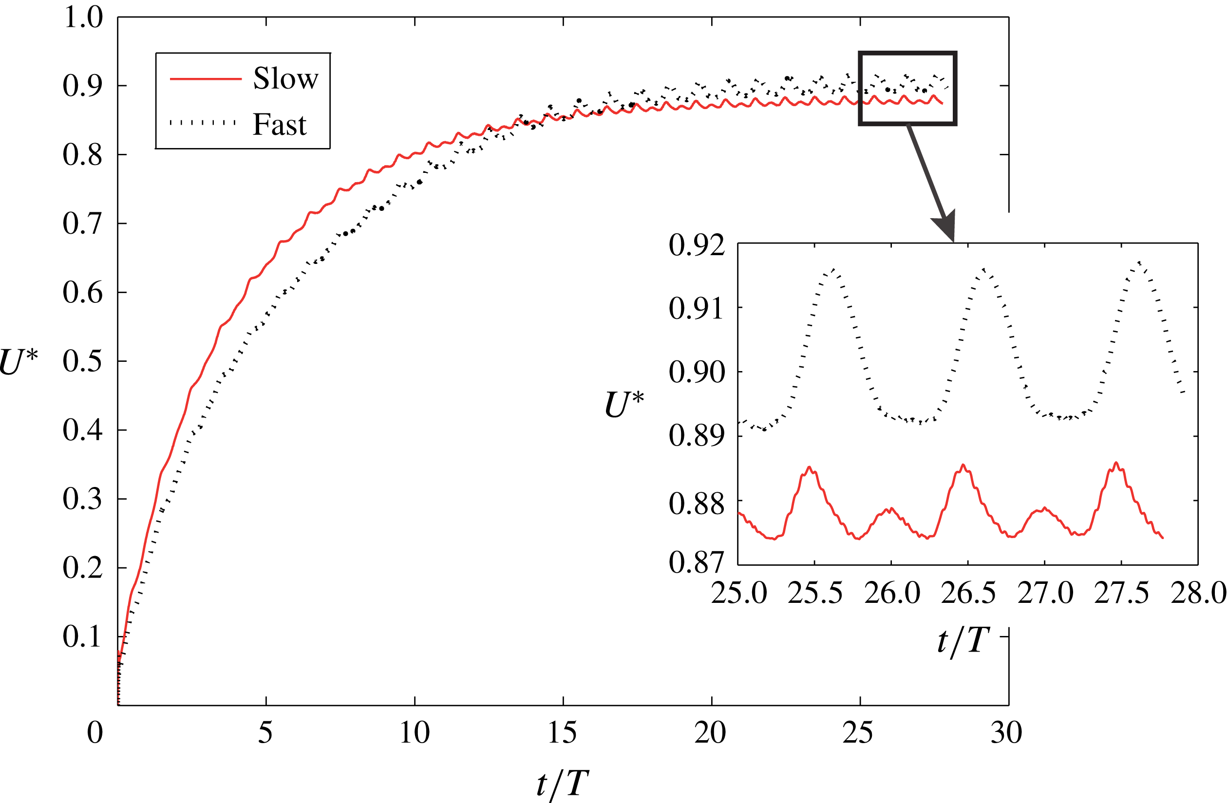
The self-propelled simulations are carried out for both slow and fast cases, and the calculated swimming speed
 $U^{\ast }$
, non-dimensionalized by the swimming speed in experiments, is shown in figure 7. The swimmers start from rest, and as they start their body motion the swimming speed increases until it reaches the quasi-steady state, at which the average swimming speed is constant. The average swimming speed
 $\overline{U^{\ast }}$
is close to one (figure 7), which indicates good agreement between the calculated swimming speed and the nominal swimming speed
 $U$
because
 $U^{\ast }$
is non-dimensionalized with
 $U$
. In fact, it is 0.9 for the fast case and 0.88 for the slow case (see table 1). This indicates approximately 10 % and 12 % difference for the fast and slow cases, respectively, in the calculated swimming speed relative to the swimming speed in the experiments from which the kinematics are derived. Such differences are reasonable considering the large standard deviations in the kinematics, e.g. see frequency
 $f$
, wavenumber
 $k$
, amplitude
 $A$
and length of the fish
 $L$
in § 2.2. For example, the
 $St$
calculated based on these values is
 $0.34\pm 0.037$
and
 $0.27\pm 0.041$
for slow and fast cases, respectively. These standard deviations are approximately 10.9 % of the nominal
 $St$
for the slow speed case and 15.3 % for the fast case, which are of the same order of magnitude as the deviations of the calculated speed from the nominal speed.
Calculated non-dimensional swimming speed
 $U^{\ast }$
for slow (
 $Re=13\,500$
,
 $St=0.34$
) and fast (
 $Re=23\,000$
,
 $St=0.27$
) cases. The inset shows the velocity fluctuations in the last cycles.

Swimming velocity during the quasi-steady state is not constant, and fluctuates slightly around the average swimming speed (figure 7). The inset in figure 7 shows more closely the velocity fluctuations, which are approximately 0.5 % and 1.5 % of
 $\overline{U^{\ast }}$
for slow and fast cases, respectively, i.e. the fast case has slightly higher fluctuations. In addition, the slow case has two peaks per cycle while the fast case has only one peak per cycle. Because the swimming speed is the integral of the acceleration of the swimmer, the difference in the time history of the hydrodynamic force, which is directly proportional to the acceleration of the swimmer, equation (2.6), creates different swimming fluctuations.
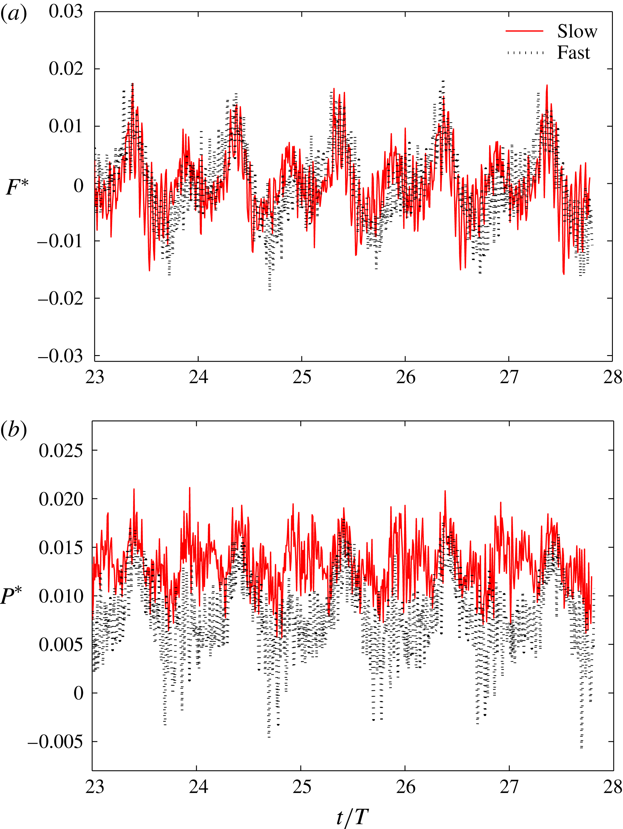
The time history of the force and power coefficients are shown in figure 8. The positive values of force are in the thrust direction (thrust type) and the negative values are in the drag direction (drag type). There are high-frequency oscillations in the force history which are much higher than those in the previous simulations (Borazjani & Sotiropoulos Reference Borazjani and Sotiropoulos2008, Reference Borazjani and Sotiropoulos2009, Reference Borazjani and Sotiropoulos2010) using the same method at lower
 $Re$
or with the inviscid assumption (no-flux through instead of no-slip condition) mainly because of the turbulence in the LES simulations at these realistic
 $Re$
values. It can be observed that the force coefficient for the slow case has two local maxima and two local minima, whereas the fast case has only one maximum and one minimum. In fact, at the beginning of each cycle, e.g.
 $t/T=27$
, the force coefficient has an inflection point and continues to increase, whereas the force coefficient for the slow case decreases to reach a local minimum. The other local maxima and minima occur almost at the same time instant in the cycle. The reasons behind such differences in the hydrodynamic force time history will be clarified by examining the wake and vortical structures in the fast and slow cases in the next section. Nevertheless, it can be observed that the magnitude of the force coefficient (figure 8
a) in the fast and slow cases is similar. However, the power coefficient of the slow case is generally higher than that of the fast case (figure 8
b). This can be better seen quantitatively in the average values of these coefficients.
The force coefficient (a) and power coefficient (b) for slow (
 $Re=13\,500$
,
 $St=0.34$
) and fast (
 $Re=23\,000$
,
 $St=0.27$
) stingray swimming cases.

The swimming performance (cycle-averaged values) parameters are calculated when the swimmer reaches the quasi-steady state (terminal velocity), which are reported in table 1. It can be observed that the thrust coefficient
 $\overline{T^{\ast }}$
(2.14) is similar for both fast and slow swimming cases. However, the power coefficient
 $\overline{P^{\ast }}$
in the fast case is almost half of that in the slow case. This can be explained by the fact that during quasi-steady state the thrust balances drag forces, and these forces in the swimming (
 $z$
) direction are mainly a function of
 $Re$
, which do not vary much for
 $Re>10\,000$
in the inertial regime. In fact, the average viscous drag coefficient is 0.0037 and 0.0032 for slow and fast swimming cases, respectively. In contrast, the power coefficient
 $\overline{P^{\ast }}$
(2.15) depends on the velocity of the body in the lateral direction relative to the swimming speed, i.e.
 $St$
number, when the amplitudes of undulations (
 $A_{x}$
and
 $A_{y}$
in (2.3)–(2.4)) are similar in both cases. The
 $St$
for the fast case is smaller than for the slow case, which results in smaller power coefficient
 $\overline{P^{\ast }}$
. This trend is in agreement with previous simulations of mackerel (Borazjani & Sotiropoulos Reference Borazjani and Sotiropoulos2008, Reference Borazjani and Sotiropoulos2009, Reference Borazjani and Sotiropoulos2010), which showed the decrease in lateral power coefficient as
 $St$
was decreased.
The lower power consumption of the fast case results in the higher efficiency of the stingray in terms of both Froude efficiency
 ${\it\eta}_{f}$
and power efficiency
 $\overline{U^{\ast }}/\overline{P^{\ast }}$
(table 1). Power efficiency
 $\overline{U^{\ast }}/\overline{P^{\ast }}$
can be considered as the power required to reach a certain velocity, similar to the concept of fuel economy (miles per gallon) in cars. It can be observed that the fast case (lower
 $St$
and higher
 $Re$
relative to the slow case) has almost double the power efficiency of the slow cases. Again, this trend is in agreement with our previous simulations, in which we observed an increase in the efficiency as
 $Re$
was increased and
 $St$
was decreased for mackerel (Borazjani & Sotiropoulos Reference Borazjani and Sotiropoulos2008, Reference Borazjani and Sotiropoulos2010). These differences in performance are related to the wake. Therefore, we investigate the wake generated by the slow and fast cases in the next subsection.
3.2. Wake structure and the pressure field
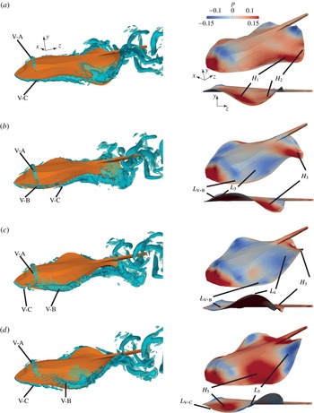
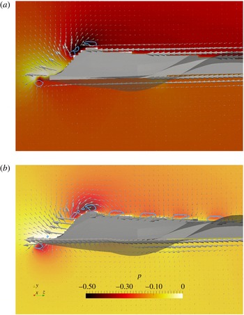
We investigate vortex dynamics during stingray swimming by visualizing flow structures using the isosurfaces of
 $q$
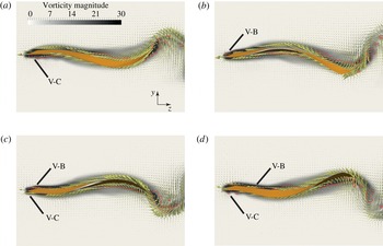
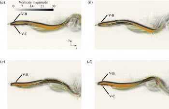
-criteria (figures 9 and 10). On the same figures, we also visualize the pressure on the surface of the stingray geometry to relate the vortical structures generated by body and wing motion to the pressure on the stingray surface, which generates the hydrodynamic thrust force. Furthermore, we visualize the footprints of
 $q$
-criteria along with the flow on the midplane of the stingray (figure 11) and the midplane of the stingray wing (figures 12 and 13). The pressure force on the stingray is along the normal direction to the surface. Therefore, the angle that a surface makes with the swimming direction (defined as angle
 ${\it\theta}$
in figure 1) determines how much of the pressure force is in the swimming (thrust) direction, e.g. a surface parallel to the swimming direction does not contribute to thrust and drag, but if it is perpendicular to the swimming direction all the pressure force is in the swimming direction. The angles that the wing geometry make with the swimming direction are better observed in these planar views (figures 12 and 13). Note that the pressure distribution on the surface is the result of several mechanisms, such as the acceleration of the adjacent fluid (added mass), and the flow circulation around the stingray wings. We try to identify the dominant mechanisms by investigating the vortical structures along with the pressure on the surface (figures 9–13) as well as the hydrodynamic force history (figure 8
a) for both slow and fast swimming cases.
Flow visualization for the slow case (
 $Re=13\,500$
,
 $St=0.34$
): 3D vortical structures visualized with the isosurfaces of
 $q$
-criteria (left-hand column, see also supplementary movie 1 available at http://dx.doi.org/10.1017/jfm.2015.702) along with pressure contours on the surface of the stingray from perspective and side views (right-hand column) at different time instants in the cycle: (a)
 $t/T=27$
, (b)
 $t/T=27.25$
, (c)
 $t/T=27.5$
, and (d)
 $t/T=27.75$
.

Flow visualization for the fast case (
 $Re=23\,000$
,
 $St=0.27$
): 3D vortical structures visualized with the isosurfaces of
 $q$
-criteria (left-hand column, see also supplementary movie 2) along with pressure contours on the surface of the stingray from perspective and side views (right-hand column) at different time instants in the cycle: (a)
 $t/T=27$
, (b)
 $t/T=27.25$
, (c)
 $t/T=27.5$
, and (d)
 $t/T=27.75$
.

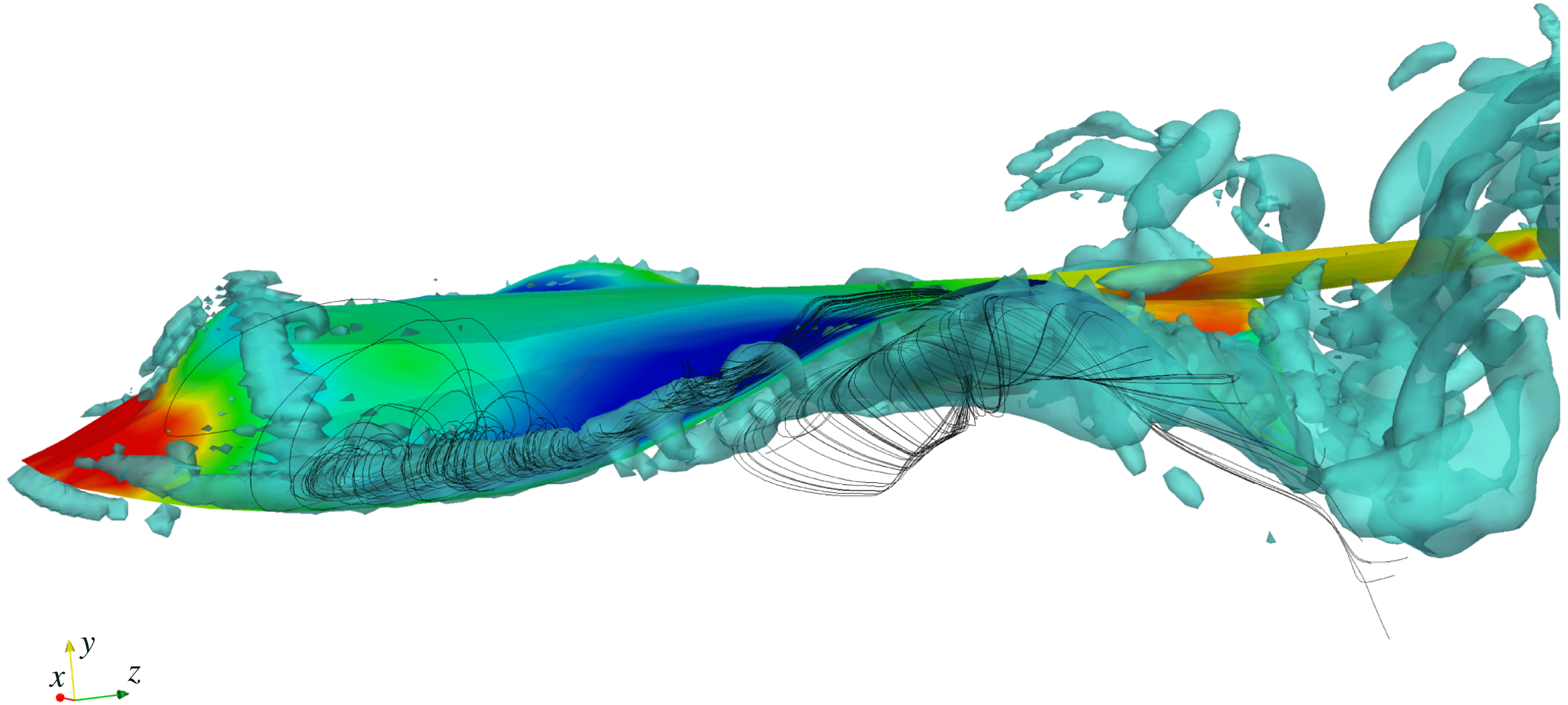
For both cases, a horseshoe vortex is generated at the nose of the stingray, which stays attached throughout the cycle (denoted by vortex V-A in figures 9 and 10). At the same time a low-pressure region is also present at all times in the frontal region of the stingray underneath this vortex (figures 9 and 10). This low-pressure region can be due to either the horseshoe vortex or the curvature of the body, i.e. the flow over curved bodies accelerates and its pressure reduces, similar to flow over airfoils. To identify which is the case, we have plotted the pressure contours and velocity vectors on the midplane of the stingray along with the footprint of the
 $q$
-criteria on that plane in figure 11. It can be observed that the regions enclosed by the
 $q$
-lines have low pressure in both high curvature (footprints of the horseshoe vortex) and low curvature (footprint of vortex V-C just below the front of the stingray). Furthermore, if the pressure was mainly dominated by the curvature, then after the peak the pressure would have steadily increased. However, after the peak the pressure does not increase steadily and remains almost constant in the figure 11(a), and increase and decrease because of the vortices in figure 11(b). Therefore, the low pressure is mainly due to the horseshoe vortex and not to the curvature of the stingray body. The low-pressure region is stronger (lower pressure) in the fast case relative to the slow case (figures 9 and 10). In addition, it is stronger when it is connected to the vortex created at the leading edge of the wing (vortex V-B) in both cases. Nonetheless, the low-pressure region in the front of the stingray, created by the horseshoe vortex at all times, enhances the hydrodynamic force in the thrust direction.
Pressure contours and velocity vectors along with the footprints of
 $q$
-criteria (thick blue lines) are plotted on the midplane of the stingray at
 $t/T=27.5$
for (a) the slow swimming case (
 $Re=13\,500$
,
 $St=0.34$
) and (b) the fast swimming case (
 $Re=23\,000$
,
 $St=0.27$
). For clarity, only every other velocity vector is plotted, and the stingray body has been made transparent.

In the slow swimming case at the beginning of the cycle (figure 9
a), there are no vortical structures on the top of the leading edge of the wing. However, there is a vortical structure (denoted by vortex V-C in figure 9
a) on the bottom side of the leading edge. Vortex V-C is connected to the tip vortex, which is being shed into the wake. To better visualize this vortex, the flow on a plane passing through the middle of the wing is visualized in figure 12(a). There is a low-pressure region due to the vortex V-C underneath the leading edge (figure 9
a), which contributes to drag. However, this contribution is small because the leading edge is almost parallel to the swimming direction at this time instant (figure 12
a). The high pressure on the top side of the front half of the wing contributes to thrust (denoted by
 $H_{1}$
in figure 9
a), but the high pressure on the top side in the back half of the wing cancels that out and contributes to drag (denoted by
 $H_{2}$
in figure 9
a). Therefore, overall the net force at this instant is near zero (figure 8
a) for the slow swimming case.
Flow visualization for the slow swimming case (
 $Re=13\,500$
,
 $St=0.34$
): vorticity magnitude and velocity vectors along with the footprints of
 $q$
-criteria (thick red lines) are plotted on the midplane of the wing at different time instants in the cycle: (a)
 $t/T=27$
, (b)
 $t/T=27.25$
, (c)
 $t/T=27.5$
, and (d)
 $t/T=27.75$
. For clarity, only every other velocity vector is plotted.

Flow visualization for the fast swimming case (
 $Re=23\,000$
,
 $St=0.27$
): vorticity magnitude and velocity vectors along with the footprints of
 $q$
-criteria (thick red lines) are plotted on the midplane of the wing at different time instants in the cycle: (a)
 $t/T=27$
, (b)
 $t/T=27.25$
, (c)
 $t/T=27.5$
, and (d)
 $t/T=27.75$
. For clarity, only every other velocity vector is plotted.

For the fast swimming case, at the beginning of the cycle (figure 10
a) an LEV (vortex V-B), in contrast to the slow swimming case, is starting to form on the top side of the leading edge, whereas vortex V-C on the bottom side of the leading edge is starting to diminish. The footprints of these vortices can be viewed in figure 13(a). There is a low-pressure region underneath vortex V-B (denoted by
 $L_{V\text{-}B}$
in figure 10
a), which does not exist in the slow swimming case. Nevertheless, the angle of the leading edge relative to the swimming direction is close to zero. Consequently, the low-pressure region created by LEVs does not contribute much to thrust. The high pressure on the top side of the front half of the wing (denoted by
 $H_{1}$
in figure 10
a) and the low pressure on the top side in the back half of the wing (denoted by
 $L_{2}$
in figure 10
a) contribute to thrust. Therefore, the total force on the stingray is in the thrust direction (figure 8
a) for the fast swimming case.
After a quarter of a cycle at
 $t/T=27.25$
in the slow swimming case, the vortex V-B is completely visible (figure 9
b). However, vortex V-C has almost diminished on the leading edge but still exists on the tip of the wing (figure 9
b). The flow on the midplane does not show vortex V-C at the leading edge either, but V-B is present (figure 12
b). Underneath vortex V-B is a low pressure in the front of the wing (denoted by
 $L_{V\text{-}B}$
in figure 9
b). In addition, the front of the wing also has a low-pressure region (denoted by
 $L_{3}$
in figure 9
b) in a location where there are no visible vortices. There is also a high-pressure region on the back of the wing (denoted by
 $H_{3}$
in figure 9
b). The angle of the wing surface with the swimming direction at this instant is such that the pressure force by
 $L_{V\text{-}B}$
,
 $L_{3}$
and
 $H_{3}$
has a component in the thrust direction (enhances thrust). Therefore, the total force on the stingray is in the thrust direction for the slow swimming case at this instant (figure 8
a).
At time instant
 $t/T=27.25$
in the fast swimming case, the vortex V-B has grown relative to the start of the cycle and the vortex V-C has diminished at the leading edge (figure 10
b). The flow on the midplane also shows vortex V-B, but not the vortex V-C at the leading edge (figure 13
b) similar to the slow swimming case (figure 12
b). Underneath vortex V-B is a low-pressure region in the front of the wing (denoted by
 $L_{V\text{-}B}$
in figure 10
b). In addition, the front of the wing also has a low-pressure region (denoted by
 $L_{3}$
in figure 10
b), and the back of the wing has a high-pressure region (denoted by
 $H_{3}$
in figure 10
b). Considering all these regions and their angles with the swimming direction (figure 10
b), the total force on the stingray is in the thrust direction for the fast swimming case at this instant (figure 8
a).
Although at this time instant (
 $t/T=27.25$
) the force on both fast and slow swimming stingrays is of thrust type, there are differences in the way this thrust is produced. In both cases the low-pressure region
 $L_{V\text{-}B}$
is created by the LEV V-B (figures 9
b and 10
b). In contrast, the low- and high-pressure regions,
 $L_{3}$
and
 $H_{3}$
, respectively (figures 9
b and 10
b), are mainly due to the added-mass effect (acceleration of the adjacent fluid) created by the propulsive wave (2.4) on the wings of the stingray. Comparing
 $L_{V\text{-}B}$
,
 $L_{3}$
and
 $H_{3}$
in fast swimming (figure 10
b) and slow swimming (figure 9
b), it can be observed that
 $L_{V\text{-}B}$
has a lower pressure in the fast swimming case, whereas
 $L_{3}$
is lower and
 $H_{3}$
is higher in the slow case. This shows that the contribution of pressure regions created by the undulatory motion (
 $L_{3}$
and
 $H_{3}$
) relative to the contribution of the LEV through the
 $L_{V\text{-}B}$
region to thrust at this time in the cycle is higher for the slow swimming case than the fast swimming case. In fact, comparing the thrust produced by the front half of the wing (
 $z<L/2$
,
 $z$
is the axial direction) to the back half of the wing (
 $z\geqslant L/2$
) shows that in the slow swimming case the back half produces 61 % more than the front half, whereas in the fast swimming case the back half only produces 15 % more. Note that the integration surface is the complete surface of the stingray’s body divided into two halves (front and back) at
 $z=L/2$
.
Another look at the force time history in figure 8(a) shows that the main difference between forces in the slow and fast swimming cases is in a time window between the start of the cycle, e.g. time instant
 $t/T=27$
, to one-quarter into the cycle, e.g.
 $t/T=27.25$
. During this time, the force in the slow swimming case has a local minimum at approximately
 $t/T=27.1$
, whereas the fast swimming case does not have this local minimum. As discussed in the previous section, this additional local minimum in the force generates the additional peaks in the swimming speed in the slow swimming case. Now, based on the above discussion on the wake structure, we can identify the origin of this local minimum. The main difference between the slow swimming and fast swimming cases at the beginning of the cycle is the existence of vortex V-B in fast swimming (figure 13
a) but not in slow swimming (figure 12
a), which affects the force history. In the slow swimming case, there is no vortex V-B at the beginning of the cycle (figure 12
a) and vortex V-C contributes to drag by creating a low-pressure region behind the leading edge as the angle between the leading edge and the swimming direction increases after
 $t/T=27$
. This creates the local minimum in the force history (drag type) at around
 $t/T=27.1$
, after which vortex V-C starts to diminish and vortex V-B, which enhances thrust, starts to form until a quarter into the cycle, when there is no vortex V-C but the vortex V-B is present (figure 12
b). In the fast swimming case, in contrast, the vortex V-B is already formed at the beginning of the cycle (figure 13
a), which contributes to thrust as the angle increases, and vortex V-C, which contributes to drag, is diminished earlier than the slow swimming case. Therefore, the thrust by vortex V-B cancels out the drag by vortex V-C, and the local minimum of drag type is not formed in the fast swimming case between
 $t/T=27$
(figure 13
a) and
 $t/T=27.25$
(figure 13
b).
At half a cycle in the slow swimming (figure 9
c), vortex V-B has grown relative to the quarter cycle, and a new vortex V-C is starting to appear at the leading edge. The footprints of these vortices are better observed in figure 12(c), which shows a small vortex V-C but a much larger V-B. Underneath vortex V-B is a low-pressure region (denoted by
 $L_{V\text{-}B}$
in figure 9
c). In addition, the front and over the hump of the wing has a low-pressure region (denoted by
 $L_{4}$
in figure 9
c), and the back of the wing has a high-pressure region (denoted by
 $H_{3}$
in figure 9
c). The surface near
 $L_{V\text{-}B}$
is almost parallel to the swimming direction, thus does not contribute much to thrust. Because the low-pressure region
 $L_{4}$
extends over the hump to the back of the wing, it reduces the effect of low pressure in front of the hump, i.e. its contribution to the thrust is reduced. The main contribution to the thrust at this time instant comes from the high-pressure region at the back of wing
 $H_{3}$
. In fact, the back half of the wing contribution to thrust is two-fold higher than the contribution of the front half of the wing. Overall, the total force on the stingray is close to zero in the thrust direction at this instant (figure 8
a).
At half a cycle in the fast swimming (figure 10
c), vortex V-B has grown relative to the quarter cycle, and has fully connected with the tip vortex. Vortex V-C, in contrast to slow swimming, has not formed on the leading edge yet, as can be observed in figure 13(c). There is a low-pressure region underneath vortex V-B (denoted by
 $L_{V\text{-}B}$
in figure 10
c), a high-pressure region in front of the hump of the wing (denoted by
 $H_{4}$
in figure 10
c), and another high-pressure region at the back of the wing (denoted by
 $H_{3}$
in figure 10
c). The surface near
 $L_{V\text{-}B}$
is almost parallel to the swimming direction, thus only contributes slightly to thrust. The high-pressure region
 $H_{4}$
in front of the hump of the wing contributes to drag, whereas the high-pressure region at the back of hump
 $H_{3}$
contributes to thrust. These two contributions from
 $H_{3}$
and
 $H_{4}$
cancel each other out for the total force on the stingray to be close to zero in the thrust direction at this instant (figure 8
a).
The force history in figure 8(a) shows that the thrust peak is in between the quarter (
 $t/T=27.25$
) and half cycle (
 $t/T=27.5$
) instants at around
 $t/T=27.4$
. The reason for this force peak is that both the low- and high-pressure regions,
 $L_{V\text{-}B}$
and
 $H_{3}$
, respectively, observed in figures 9(b,c) and 10(b,c) contribute to thrust within this time window. In this time window, the angle of the leading-edge surface with the swimming direction makes the pressure force due to
 $L_{V\text{-}B}$
have a component in the swimming direction, while the high-pressure region
 $H_{3}$
at the back of the wing has a component in the thrust direction and pushes the stingray forwards. The high-pressure region
 $H_{3}$
is created by the added-mass (reactive force) effect because of the acceleration of the adjacent fluid due to the undulatory motion. The added-mass force is higher in the back of the wing due to larger undulations, which result in higher accelerations of the surface and the adjacent fluid. The low-pressure region
 $L_{V\text{-}B}$
enhances thrust because of the LEV V-B in front of the wing. Although these two mechanisms are present in both slow and fast swimming, their contributions are different in these two swimming conditions. The contribution of the back half of the wing relative to its front half is much higher in the slow swimming case. For example, at time instant
 $t/T=27.25$
, the back half contributes 61 % and 15 % more than the front half in slow and fast swimming, respectively; and at time instant
 $t/T=27.5$
, it contributes 218 % and 77 % more than the front half in slow and fast swimming, respectively. Therefore, the low-pressure region caused by the LEV V-B enhances thrust in fast swimming more than in slow swimming.
At three-quarters into the cycle for slow swimming (figure 9
d), vortex V-B has shrunk and moved away from the leading edge, but vortex V-C has grown relative to the half cycle (figure 9
c). The larger size of vortex V-C and smaller size of vortex V-B are better observed in figure 12(d). There is a low-pressure region beneath the leading edge where vortex V-C is visible (denoted by
 $L_{V{-}C}$
in figure 9
d). In addition, there is a low-pressure region in the back of the wing (denoted by
 $L_{5}$
in figure 9
d), and a high-pressure region at the trough of the wing (denoted by
 $H_{5}$
in figure 9
d). The angles that these surfaces,
 $L_{V{-}C}$
,
 $H_{5}$
and
 $L_{5}$
, make with the swimming direction are such that the pressure force on these surfaces has a component in the swimming direction. Nevertheless, the back half of the wing contributes more than three times the front half of the wing to thrust at this time instant.
At three-quarters into the cycle for fast swimming (figure 10
d), vortex V-B is diminishing while vortex V-C is forming at the leading edge. The footprints of these vortices on the midplane of the wing, shown in figure 13(d), also show the formation of the vortex V-C, which could not be observed at the half cycle (figure 13
c). Because vortex V-C is not as strong as for the slow swimming at this instant, it does not create a strong low-pressure region at the leading edge. Nevertheless, there is a low-pressure region in the middle of the wing (denoted by
 $L_{5}$
in figure 10
d), a high-pressure region in the front of the wing (denoted by
 $H_{5}$
in figure 10
d), and another high-pressure region in the posterior region of the wing (denoted by
 $H_{6}$
in figure 10
d). The angles that the surfaces
 $H_{5}$
make with the swimming direction are such that the pressure force on it has a component in the swimming direction. However,
 $H_{6}$
, which has higher area with higher pressure, contributes to drag;
 $L_{5}$
is almost at the valley of the wing, where the angle with the swimming direction is almost zero. Thus, the
 $L_{5}$
contribution to thrust is small. Overall, the total force on the stingray is of drag type at this instant (a negative force value in figure 8(a) at this instant).
Here, we have discussed the wake structure along with the pressure and forces for one wing-beat cycle. In the next section, we discuss the thrust generation mechanisms and the contribution of the LEV in ray-like swimming.
4. Discussions and conclusions
4.1. Contribution of the leading-edge vortex to thrust
As discussed in the Introduction, there are two main mechanisms in aquatic propulsion (figure 1): the added-mass (reactive force) mechanism, and the lift-based (vorticity, circulatory) mechanism. The added-mass mechanism is observed in undulatory swimming, whereas the lift-based mechanism is observed in oscillatory (heaving and pitching) swimming.
The main parameter that controls the force generation using the added-mass mechanism in undulatory swimming is the so-called slip velocity or slip ratio defined as
 $U/V$
, where
 $V$
is the velocity of the propulsive wave that propagates backwards on the stingray’s wings and
 $U$
is the swimming speed (Lighthill Reference Lighthill1960). In fact, when the lateral velocity at the trailing edge is
 $W$
, the water near the trailing edge is pushed to the side with a speed much lower than
 $W$
equal to
 $w=W(V-U)/V<W$
– see figure 5 of Lighthill (Reference Lighthill1969) for a simple explanation. It can be observed that
 $w$
(consequently, the added-mass force – see appendix B) becomes larger as
 $U/V$
decreases and tends to zero as
 $U/V$
tends towards one as the fish would be slipping through water without giving it any lateral displacement.
The main parameter that governs the lift-based mechanism is the circulation
 ${\it\Gamma}$
around the foil/wing. In fact, the lift force is
 $L={\it\rho}U{\it\Gamma}$
, where
 ${\it\rho}$
is the density of the fluid. There are several mechanisms that enhance the circulation and the generated lift, e.g. clap and fling (Weis-Fogh Reference Weis-Fogh1973), wing–wake interaction (Birch & Dickinson Reference Birch and Dickinson2003) and the LEV (Ellington et al.
Reference Ellington, Van Den Berg, Willmott and Thomas1996) – see the review by Sane (Reference Sane2003). In hovering insects and slow flying birds, the contribution from LEV to the lift is thought to be significant. Ellington et al. (Reference Ellington, Van Den Berg, Willmott and Thomas1996) estimated the contribution of the LEV by assuming that the difference between the lift predicted by the steady aerodynamics and the weight of the hawkmoth is produced by the LEV, i.e. the theoretical estimate was around 20 % lower than the weight, which was assumed to be the contribution from the LEV because the theory did not consider LEV. This approach cannot be used to estimate the contribution of the LEV in aquatic swimming because the theoretical estimates of thrust using elongated-body theory (Lighthill Reference Lighthill1971) or other inviscid methods (Newman & Wu Reference Newman and Wu1975; Wu Reference Wu2011), which do not account for the presence of the LEV, tend to overestimate the thrust by several-fold. In fact, the mean thrust coefficient for the stingray based on elongated-body theory is found to be much larger than the calculated viscous drag coefficient from the simulations as shown in appendix B. Thus, the theoretical thrust (which does not consider LEV) is typically higher (not lower) than what is measured experimentally or calculated numerically (which considers LEV), and cannot be used to estimate the LEV contribution. If the theory underestimated the thrust, then the underestimated amount could have been contributed to the LEV.
Another method to estimate the contribution of the LEV is to compare the circulation within the LEV to the total circulation around the wing (Muijres et al. Reference Muijres, Johansson, Barfield, Wolf, Spedding and Hedenström2008; Thielicke & Stamhuis Reference Thielicke and Stamhuis2015). Muijres et al. (Reference Muijres, Johansson, Barfield, Wolf, Spedding and Hedenström2008) estimated LEV to increase the lift as much as 40 % during slow flight of bats by showing that the ratio of the circulation of the leading to the trailing vortex is around 40 %. Nevertheless, this method cannot be used in aquatic swimming because the cycle-averaged force (circulation) during self-propelled swimming is zero and not a positive value as in insect/bird flight. Anderson et al. (Reference Anderson, Streitlien and Barrett1998) stated that the timing of the shedding of the vortices at the leading edge affects propulsive efficiency whether they interact constructively or destructively with the trailing vortices. Lewin & Haj-Hariri (Reference Lewin and Haj-Hariri2003) also observed that when the LEV gets separated the efficiency of heaving foils decreases. Dong et al. (Reference Dong, Mittal and Najjar2006) also mentioned the importance of the LEV for efficiency. However, none of these foil studies quantify the contribution of the LEV relative to the total force and qualitatively correlated the efficiency with LEV dynamics (Anderson et al. Reference Anderson, Streitlien and Barrett1998; Lewin & Haj-Hariri Reference Lewin and Haj-Hariri2003; Dong et al. Reference Dong, Mittal and Najjar2006). Based on the above discussion, we need another method to quantify the contribution of the LEV to thrust.
Stingray swimming is in undulatory mode, which is known to suppress flow separation (Taneda & Tomonari Reference Taneda and Tomonari1974; Shen et al.
Reference Shen, Zhang, Yue and Triantafyllou2003; Borazjani & Sotiropoulos Reference Borazjani and Sotiropoulos2008). The experiments on a mechanical, undulatory ray wing also did not report any flow separation on the wing (Clark & Smits Reference Clark and Smits2006). Nevertheless, we observed a vortex at the leading edge (vortex V-B in figures 9 and 10) that can enhance thrust. Because of the undulatory swimming of the stingray, the added-mass mechanism is thought to be the main mechanism for its propulsion, which is governed by slip velocity
 $U/V$
as discussed above. The slip velocity
 $U/V$
is 0.76 and 0.89 for slow and fast swimming, respectively. If it was a completely inviscid phenomenon, the
 $U/V$
value would have remained the same because the waveform is similar and only the frequency is changed between fast and slow swimming. The higher slip velocity indicates higher added-mass (reactive) force in slow swimming. This is consistent with our results discussed in the previous section, because the majority of the low-pressure regions for the slow swimming case were in locations where there were no visible vortices, e.g. posterior and middle of the wing (figure 9
b–d). In fast swimming, in contrast, the low-pressure regions during most of the cycle were located on the leading edge from vortex V-B (figure 10
a–c). Therefore, the LEV contributes more to thrust in fast swimming than in slow swimming.
To somehow quantify the contribution of the added mass versus LEV in slow and fast swimming, we compare the thrust force created by the front half and the back half of the wing. This can be a good measure because the added-mass force is mainly generated by the back of the wing where there are higher undulations, whereas the LEV force is mainly generated by the front of the wing. For the pressure force to be independent of the reference pressure, it should be calculated over a closed surface
 $A$
, i.e.
 $\int _{A}\,\text{d}A=0$
. This condition is satisfied in calculating the force over the half wing because of the thin geometry of the wing. Comparing the forces produced by the front half and back half of the wing in slow and fast swimming, it can be observed that slow swimming consistently produces much more thrust at the back of the wing than fast swimming. For example, at
 $t/T=27.25$
the back half produced 61 % and 15 % more thrust than the front half in slow and fast swimming, respectively, and 218 % and 77 % at
 $t/T=27.5$
in slow and fast swimming, respectively. This clearly shows that in slow swimming more thrust is produced using the added-mass (reactive) mechanism by the back half of the wing, whereas in fast swimming the thrust is enhanced by the LEV at the font half of the wing. The thrust enhancement by the LEV in fast swimming is consistent with its higher efficiency than slow swimming.
4.2. Leading-edge vortex in aquatic swimming versus flying
The LEV has been observed in insect flight (Ellington et al.
Reference Ellington, Van Den Berg, Willmott and Thomas1996; Van Den Berg & Ellington Reference Van Den Berg and Ellington1997), bat flight (Muijres et al.
Reference Muijres, Johansson, Barfield, Wolf, Spedding and Hedenström2008, Reference Muijres, Johansson, Winter and Hedenström2014), bird flight (Videler et al.
Reference Videler, Stamhuis and Povel2004), plant seeds (Lentink et al.
Reference Lentink, Dickson, Van Leeuwen and Dickinson2009) and rotary machinery such as wind turbines (Tangler Reference Tangler2004; Sicot et al.
Reference Sicot, Devinant, Loyer and Hureau2008; Dumitrescu & Cardos Reference Dumitrescu and Cardos2012; Lee & Wu Reference Lee and Wu2013). However, LEV has not been reported in aquatic swimming, probably due to the overemphasis on the trailing wake and the greater ease of visualizing it in studies of live swimming fish (Barrett, Triantafyllou & Yue Reference Barrett, Triantafyllou and Yue1999; Muller, Stamhuis & Videler Reference Muller, Stamhuis and Videler2000; Nauen & Lauder Reference Nauen and Lauder2001; Liu Reference Liu2005; Clark & Smits Reference Clark and Smits2006; Kern & Koumoutsakos Reference Kern and Koumoutsakos2006; Mittal et al.
Reference Mittal, Dong, Bozkurttas, Lauder and Madden2006; Borazjani & Sotiropoulos Reference Borazjani and Sotiropoulos2008; Dong et al.
Reference Dong, Bozkurttas, Mittal, Madden and Lauder2010) and the fact that the flow does not separate along the body of undulating swimmers (Taneda & Tomonari Reference Taneda and Tomonari1974; Shen et al.
Reference Shen, Zhang, Yue and Triantafyllou2003; Borazjani & Sotiropoulos Reference Borazjani and Sotiropoulos2008). Previous simulations of Borazjani & Daghooghi (Reference Borazjani and Daghooghi2013) have provided the first evidence of a stable LEV on fish tails using 3D high-resolution numerical simulations of self-propelled virtual swimmers with different tail shapes. They showed an attached, stable LEV with high efficiency at low
 $St\approx 0.25$
, but a separated LEV with low efficiency at higher
 $St\approx 0.5$
(Borazjani & Daghooghi Reference Borazjani and Daghooghi2013). Our results here also show the existence of the LEV on the stingray wings for the first time (figures 9 and 10). The existence of the LEV on the stingray wing with undulatory motion is quite unique because undulatory motion is known to remove separation (Taneda & Tomonari Reference Taneda and Tomonari1974; Shen et al.
Reference Shen, Zhang, Yue and Triantafyllou2003; Borazjani & Sotiropoulos Reference Borazjani and Sotiropoulos2008). Quinn et al. (Reference Quinn, Lauder and Smits2014) also report stable LEV on 2D flexible foils at a very high
 $St>1$
, but vortex shedding from the leading edge at lower
 $St$
.
Considering the ubiquity of the LEV (Ellington et al.
Reference Ellington, Van Den Berg, Willmott and Thomas1996; Van Den Berg & Ellington Reference Van Den Berg and Ellington1997; Videler et al.
Reference Videler, Stamhuis and Povel2004; Muijres et al.
Reference Muijres, Johansson, Barfield, Wolf, Spedding and Hedenström2008; Lentink et al.
Reference Lentink, Dickson, Van Leeuwen and Dickinson2009; Borazjani & Daghooghi Reference Borazjani and Daghooghi2013), it can be regarded as a convergent evolutionary feature in biological propulsion systems, which should serve as an inspiration to enhance force generation/energy harvesting of man-made systems. To apply LEV dynamics in such systems, the mechanisms for generation of a stable LEV need to be understood. For translating 2D foils (Dickinson & Gotz Reference Dickinson and Gotz1993; Kim & Gharib Reference Kim and Gharib2010; Beem et al.
Reference Beem, Rival and Triantafyllou2012; Pitt Ford & Babinsky Reference Pitt Ford and Babinsky2013) or heaving and pitching 2D foils (Anderson et al.
Reference Anderson, Streitlien and Barrett1998; Wang Reference Wang2000; Lewin & Haj-Hariri Reference Lewin and Haj-Hariri2003; Dong et al.
Reference Dong, Mittal and Najjar2006), the LEV grows and starts shedding, but it remains stable/attached for 3D rotating blades (Ellington et al.
Reference Ellington, Van Den Berg, Willmott and Thomas1996; Van Den Berg & Ellington Reference Van Den Berg and Ellington1997; Aono et al.
Reference Aono, Liang and Liu2008; Lentink & Dickinson Reference Lentink and Dickinson2009a
,Reference Lentink and Dickinson
b
; Ozen & Rockwell Reference Ozen and Rockwell2012; Harbig et al.
Reference Harbig, Sheridan and Thompson2013; Cheng et al.
Reference Cheng, Roll, Liu, Troolin and Deng2014). A spanwise flow, which causes the LEV spiral towards the tip (Maxworthy Reference Maxworthy1981; Ellington et al.
Reference Ellington, Van Den Berg, Willmott and Thomas1996; Van Den Berg & Ellington Reference Van Den Berg and Ellington1997; Wang Reference Wang2005; Lentink & Dickinson Reference Lentink and Dickinson2009b
), is suggested to stabilize the LEV by providing a vorticity sink to balance the vorticity flux of the leading-edge shear layer. However, the spanwise flow was not observed for a model insect wing at low
 $Re$
(Birch & Dickinson Reference Birch and Dickinson2001), but it was observed at higher
 $Re$
(Birch et al.
Reference Birch, Dickson and Dickinson2004). Here we observe the spiral flow in the LEV in stingrays as shown in figure 14 similar to what was found for fish tails (Borazjani & Daghooghi Reference Borazjani and Daghooghi2013). Recently, vorticity annihilation due to interaction between the LEV and the opposite-sign vorticity layer has been suggested as an important mechanism for LEV stabilization (Wojcik & Buchholz Reference Wojcik and Buchholz2014). However, the conditions that lead to generation of the spiral flow or vorticity annihilation are still not well understood. Lentink & Dickinson (Reference Lentink and Dickinson2009a
,Reference Lentink and Dickinson
b
) suggest rotational acceleration, which scales with the inverse of Rossby number (
 $Ro$
), as the stabilizing mechanism on insect wings. They state that the condition for stability of the LEV is
 $Ro\approx 1$
, and at high
 $Ro$
LEV becomes unstable and sheds (Lentink & Dickinson Reference Lentink and Dickinson2009b
).
Flow visualization of the slow swimming case (
 $Re=13\,500$
,
 $St=0.34$
): the 3D vortical structures are visualized with the isosurfaces of
 $q$
-criteria. Streamlines are drawn in the region near the leading edge, which show the spiral flow of the LEV.

Despite great similarities in the structure of the LEV in hovering insects and in our results for aquatic swimmers, there are several important differences. A major difference is that in insects the rotation of the wing around its root does not change the geometric angle of attack (Lentink & Dickinson Reference Lentink and Dickinson2009a
) similar to purely rotating wings (Usherwood & Ellington Reference Usherwood and Ellington2002; Birch et al.
Reference Birch, Dickson and Dickinson2004). However, there is no such rotation in fish tails or stingray wings, and the motion can be considered as a flapping (heaving and pitching) plus an undulatory motion, which changes the geometric angle of attack at each time instant. Furthermore, the
 $Ro$
number is higher for freely swimming swimmers relative to hovering insects due to higher free swimming speed and a smaller radius of rotation, i.e. rotational acceleration (Lentink & Dickinson Reference Lentink and Dickinson2009b
) probably does not stabilize LEV in aquatic swimming. In fact, LEVs have only been seen in slow flying bats/birds (Muijres et al.
Reference Muijres, Johansson, Barfield, Wolf, Spedding and Hedenström2008; Thielicke & Stamhuis Reference Thielicke and Stamhuis2015) and hovering insects (Ellington et al.
Reference Ellington, Van Den Berg, Willmott and Thomas1996; Birch et al.
Reference Birch, Dickson and Dickinson2004), and not in freely flying ones except bumblebees (Bomphrey, Taylor & Thomas Reference Bomphrey, Taylor, Thomas, Taylor, Triantafyllou and Tropea2010), probably because of their small wings that reduce
 $Ro$
. In fact, Muijres et al. (Reference Muijres, Johansson, Winter and Hedenström2014) report that the LEV is visible during slow but not fast flight. Therefore, the stability mechanism for the LEV in aquatic swimming might be different from those in insect/bird flight, which requires further research.
4.3. Conclusions
We have carried out LES of a stingray whose motion is prescribed based on experimental measurements of the 3D body and pectoral fin kinematics in a fast and a slow swimming stingray. Swimming velocity calculated through the self-propelled simulations is within 10–12 % of the nominal experimental swimming speed. During the quasi-steady state at which the average swimming speed remains constant, the average force over the cycle is zero. The average thrust coefficients in fast and slow swimming are similar, whereas the average power coefficient of fast swimming is half that of slow swimming. Consequently, the stingray swimming at the higher speed (
 $Re=23\,000$
,
 $St=0.27$
) has approximately 12 % higher Froude efficiency and almost two times higher power efficiency than the one swimming at lower speed (
 $Re=13\,500$
,
 $St=0.34$
) – see table 1.
The main reason for this higher efficiency was found to be the higher contribution of the LEV to thrust in the fast case through the generation of a low-pressure region in front of the wing (
 $L_{V\text{-}B}$
in figure 10
b,c). We showed that the front of the wing consistently contributes more to the total thrust in fast swimming than in slow swimming, as discussed in § 4.1. The added-mass (reactive) force, which generates thrust by the acceleration of the adjacent fluid by the backward-travelling wave on the fish’s body, is higher in the back of the wing because of higher undulations and velocities. The higher force generation by the back of the wing in slow swimming through the added-mass mechanism is consistent with the low- and high-pressure regions on the posterior sections of the wing, which were not close to the vortical structures (
 $L_{3,4}$
and
 $H_{3,4}$
in figure 9
b,c). The horseshoe-like vortex on the nose of the stingray created a low-pressure region in the front of the stingray for both cases at all times which enhanced thrust (V-A in figures 9 and 10). The presence of the horseshoe vortex is due to the shape of the ray’s head (figure 11). The effect of a smoother and streamlined shape which does not allow separation (but creates a lower-pressure region through curvature) on the hydrodynamic force is not investigated here. Therefore, we cannot comment on the efficiency/benefit of enhancing the hydrodynamic force in the thrust direction through a horseshoe vortex relative to other means.
The fast swimming stingray had higher velocity fluctuations than the slow swimming one (figure 7). The reason behind the higher velocity fluctuations is a higher contribution of the LEV in thrust generation during fast swimming. The LEV contributes in only part of the cycle (vortex V-B in figure 10 a,b), whereas the added-mass mechanism continuously generates thrust by accelerating the adjacent fluid. The mackerel-like swimmers, which generate LEV on their tails (Borazjani & Daghooghi Reference Borazjani and Daghooghi2013), also have higher velocity fluctuations than the eel-like swimmers, which generate thrust using the added-mass mechanism by their undulatory motion (Borazjani Reference Borazjani2015).
The velocity and force history in the slow swimming case shows two peaks per cycle, but there is only one peak in fast swimming. In fact, the beginning of the cycle, e.g.
 $t/T=27$
, is an inflection point in fast swimming, after which the force increases, but in slow swimming the force decreases and reaches a minimum. We found the reason for this force decrease after the start of the cycle in slow swimming to be the existence of a vortex underneath the leading edge (vortex V-C in figure 12
a), which contributes to drag by generating a low-pressure region behind the leading edge. Instead, in fast swimming the vortex underneath is diminishing (vortex V-C in figure 13
a) and a vortex above the leading edge (vortex V-B in figure 13
a) forms, which contributes to thrust and cancels out the effect of vortex V-C.
The spanwise/spiral flow through the centre of the LEV, which is thought to stabilize the LEV by convecting the vorticity out of the LEV, was observed on the stingray wings as well (figure 14). Nevertheless, the stability mechanism of the LEV formed on fish tails and stingray wings during self-propelled swimming might be different from the LEV in hovering insects or the slow flight of birds/bats because of the high Rossby numbers in free swimming, as discussed in the previous section. Investigating the stability mechanisms of the LEV in aquatic swimming will be pursued as part of future work.
Acknowledgements
We thank V. Vruddhula (B.Sc., SUNY Buffalo) for helping with the generation of the stingray geometry. This work was partially supported by the Center for Computational Research (CCR) at the University at Buffalo, and the Western New York Prosperity Scholarship (R.G.B.). This work was supported in part by National Science Foundation grants CBET 1453982 to I.B., and EFRI-0938043 and CDI 0941674 to G.V.L. We thank the anonymous reviewers for their comments that improved this paper.
Supplementary movies
Supplementary movies are available at http://dx.doi.org/10.1017/jfm.2015.702.
Appendix A. LES of flow over a cylinder
We carry out LES of the flow over a cylinder at
 $Re=3900$
, which is considered a canonical test case for LES (Beaudan & Moin Reference Beaudan and Moin1994; Mittal & Moin Reference Mittal and Moin1997; Breuer Reference Breuer1998; Jordan Reference Jordan1999; Kravchenko & Moin Reference Kravchenko and Moin2000). The computational grids used for the simulations are a
 $3D\times 10L\times 15D$
box, where
 $D$
is the diameter of the cylinder, in the
 $x$
,
 $y$
and
 $z$
directions, respectively. The length of the cylinder is the
 $x$
direction. The centre of the cylinder is positioned
 $5D$
from the inlet in the
 $z$
direction and was centred in the
 $y$
direction. The inlet is a uniform flow (with no turbulence), and the outlet is a far-field (Neumann) boundary condition with a correction to satisfy the conservation of mass. The boundary conditions in the
 $x$
and
 $y$
directions are slip walls. The
 $x$
–
 $y$
–
 $z$
directions are discretized with two grids: one with
 $101\times 201\times 301\approx 6.0$
million nodes and another with
 $101\times 253\times 349\approx 8.9$
million nodes. The region directly surrounding the cylinder comprised a
 $3D\times D\times D$
cuboid discretized with a uniform grid spacing of
 $h=0.02D$
and
 $h=0.01D$
for the coarse and fine grids, respectively. The grid was stretched from the uniform cuboid to the outer edges of the computational domain using a hyperbolic tangent function. The non-dimensional time step was set to 0.02 for simulations on both grids.
Flow visualization of LES of a cylinder (
 $Re=3900$
): the 3D vortical structures are visualized with the isosurfaces of
 $q$
-criteria for (a) the time-averaged flow and (b) the instantaneous flow.

The simulations are carried out at
 $Re=3900$
and 8000 to compare with the experimental data. They are initialized with uniform flow, the time averaging is started when the total kinetic energy of the domain reaches quasi-steady, and the simulations are continued until the average quantities do not vary much as the averaging continues. The instantaneous and the time-averaged flows over the cylinder are visualized using isosurfaces of
 $q$
-criteria in figure 15. The unsteady vortex shedding is observed in the instantaneous flow field, while the separated region is observed in the time-averaged flow in figure 15. The time-averaged wake for
 $Re=3900$
is compared against the experimental measurements of Ong & Wallace (Reference Ong and Wallace1996) and Lourenco & Shih (Kravchenko & Moin Reference Kravchenko and Moin2000) in figure 16. The velocity in the axial direction on the centreline of the wake behind the cylinder shows that the finer grid (
 $h=0.01D$
) can capture the separation region more accurately than the coarse grid. The velocity outside the separation region (
 $z/D>3$
) and the peak backward velocity are similar on both grids. Comparison of the pressure coefficient on the cylinder against experimental data of Norberg (Reference Norberg1987) in figure 17 shows that our CURVIB method can capture the pressure accurately on the cylinder at both
 $Re$
3900 and 8000.
Streamwise velocity on the centreline in the wake of a circular cylinder at
 $Re=3900$
. The experimental results of Ong & Wallace (Reference Ong and Wallace1996) and Lourenco & Shih were extracted from the paper by Kravchenko & Moin (Reference Kravchenko and Moin2000).

Comparison of the pressure coefficient
 $C_{P}$
of the LES at
 $Re=3900$
and 8000 on the fine grid (
 $h=0.01D$
) with the experimental measurements of Norberg (Reference Norberg1987). Experimental data were extracted from the paper by Jordan (Reference Jordan1999).

Appendix B. Thrust force based on elongated-body theory
Here we compute the thrust force for our undulatory swimmer based on the elongated-body theory (EBT) of Lighthill (Reference Lighthill1971). According to EBT the thrust is given by (equation (11) of Lighthill Reference Lighthill1971)
 $$\begin{eqnarray}\displaystyle T=\left[mw\left(W-\frac{1}{2}w\right)\right]_{z=L}-\frac{\partial }{\partial t}\int _{0}^{L}\left(mw\frac{\partial h}{\partial z}\right)\,\text{d}z. & & \displaystyle\end{eqnarray}$$
Here
 $h$
is the displacement from the stretched straight position because of the undulations,
 $z$
is the axial direction from the head (
 $z=0$
) to the end of the tail (
 $z=L$
),
 $W=\partial h/\partial t$
is the lateral velocity,
 $w=\partial h/\partial t+U\partial h/\partial z$
is the velocity of water that is pushed laterally near the trailing edge, and
 $m$
is the virtual mass per unit length, approximated by
 $$\begin{eqnarray}\displaystyle m={\textstyle \frac{1}{4}}{\rm\pi}s^{2}{\it\rho}{\it\beta}, & & \displaystyle\end{eqnarray}$$
where
 ${\it\rho}$
is the water density,
 $s$
is the depth of the cross-section and
 ${\it\beta}$
is a non-dimensional parameter that is close to one for different cross-sections (Lighthill Reference Lighthill1971). Lighthill (Reference Lighthill1971) shows that
 $$\begin{eqnarray}\displaystyle w=W(V-U)/V, & & \displaystyle\end{eqnarray}$$
where
 $U$
is the swimming velocity and
 $V$
is the wave speed of the travelling wave. Using the fact that the mean value of the integral in (B 1) is zero, the time-averaged thrust coefficient,
 $\overline{T^{\ast }}$
is given by
 $$\begin{eqnarray}\displaystyle \overline{T^{\ast }}=\frac{\overline{T}}{{\it\rho}U^{2}L^{2}}=\left[\frac{m}{{\it\rho}L^{2}}\frac{w}{U}\left(\frac{W}{U}-\frac{1}{2}\frac{w}{U}\right)\right]_{z=L}. & & \displaystyle\end{eqnarray}$$
Substituting
 $w$
from (B 3) and
 ${\it\beta}=1$
, we get
 $$\begin{eqnarray}\displaystyle \overline{T^{\ast }}=\left[\frac{1}{8}{\rm\pi}\left(\frac{s}{L}\right)^{2}\left(\frac{W}{U}\right)^{2}\left(1-\left(\frac{U}{V}\right)^{2}\right)\right]_{z=L}. & & \displaystyle\end{eqnarray}$$
Based on the above equation, we can estimate the thrust and compare it with our numerical results. We approximate the depth
 $s/L$
of the fin to be equal to one because of the disk shape of the body. We approximate the lateral velocity by
 $W=Af$
(
 $A$
and
 $f$
are the amplitude and frequency of the undulations, respectively). Therefore, the non-dimensional
 $W/U=Af/U$
is the Strouhal number
 $St$
, which is 0.34 and 0.27 for slow and fast swimming, respectively;
 $U/V$
is the slip velocity, which is 0.76 and 0.89 for slow and fast swimming, respectively. Consequently, the mean thrust coefficient based on (B 5) is 0.019 and 0.006 for slow and fast swimming, respectively, which is much larger than the mean viscous drag coefficient of 0.0037 and 0.0032 computed numerically for the slow and fast cases, respectively.