2 The governing equations

We consider the motion induced in a semi-infinite layer of viscous fluid by a flat plate located at $y = 0$ , which undergoes in-plane oscillations. This movement occurs in the $x$ -direction with a plate velocity $U_0\cos \omega t$ . If all lengths are scaled on $\sqrt {2\nu /\omega }$ , velocities on $U_0$ , and the dimensionless time $\tau =\omega t$ is introduced, then, in the absence of disturbances, the classical Stokes layer flow is simply given by

(2.1) $$ \begin{align} u=U_B(y,\tau)=\exp(-y)\cos(y-\tau),\quad v=0, \end{align} $$

where $u$ and $v$ denote the flow velocities in the $x$ - and $y$ -directions, respectively.

The linear stability of (2.1) is found by imposing a disturbance of the form

$$ \begin{align*}(u,v)=(U_B,0)+\varepsilon\bigg(\frac{\partial\Psi}{\partial y}, -\frac{\partial\Psi}{\partial x}\bigg),\end{align*} $$

where $\varepsilon \ll 1$ and $\Psi (x,y,\tau )$ is an appropriate disturbance stream function. It is most convenient to decompose

(2.2a) $$ \begin{align} \Psi(x,y,\tau) &=\exp(iax)\exp(\mu\tau) \psi(y;\tau)+\mathrm{complex~conjugate}, \end{align} $$

where we point out that the disturbance wave number $a\in \mathbb {R}$ is supposed to be specified. We can then appeal to Floquet theory, which is concerned with the solution of differential equations with coefficients that are periodic functions of the independent variable. The key result for our purposes is that the $(y,\tau )$ -dependence of the solution can be written $\exp (\mu \tau ) \psi (y;\tau )$ , where $\psi (y;\tau )$ is $2\pi $ -periodic (in $\tau $ ). Any exponential growth or decay in $\Psi $ can be incorporated within the (complex-valued) Floquet exponent $\mu $ . Given this form for the disturbance stream function $\Psi (x,y,\tau )$ , the associated perturbation vorticity is written in the form

(2.2b) $$ \begin{align} Z=&\exp(iax)\exp(\mu\tau) \zeta(y;\tau)+\mathrm{complex~conjugate}. \end{align} $$

We note that this stability formulation has been limited to consideration of two-dimensional modes that depend only on the $x$ - and $y$ -coordinates. This is justifiable because this problem is an example of a famous result known as Squire’s theorem [Reference Squire34]. In its simplest form, this states that for a parallel shear flow of an incompressible fluid, two-dimensional perturbations become unstable at a lower $R$ than do their three-dimensional counterparts. The upshot is that the stability of the plane Stokes layer can be deduced by restricting ourselves to purely two-dimensional modes, safe in the knowledge that if all two-dimensional disturbances are stable, then necessarily so are all three-dimensional ones. In passing, we remark that a slightly more complicated oscillatory profile can be generated if orthogonal, isochronous oscillations, again in the plane of the plate, are superimposed on the basic boundary motion. Provided the two perpendicular oscillations are out of phase with each other, the plate will undergo an orbital motion and the fluid velocity will be just the linear superposition of the Stokes-layer profiles corresponding to each direction of oscillation. Even with this more intricate motion, it can be shown that Squire’s theorem continues to hold [Reference Blennerhassett and Bassom7].

With these expressions noted, the governing stream function/vorticity equations, when linearized in $\varepsilon $ , become

(2.3a) $$ \begin{align} \frac{\partial\zeta}{\partial\tau}&=\frac12\bigg(\frac{\partial^2}{\partial y^2} -a^2\bigg)\zeta-\mu\zeta-iaRU_{B}\zeta+iaRU_{Byy}\psi\,,\end{align} $$

(2.3b) $$ \begin{align} \zeta &= \bigg(\frac{\partial^2}{\partial y^2} -a^2\bigg)\psi;\end{align} $$

this system needs to be solved subject to

(2.3c) $$ \begin{align}\psi & =\psi_y=0\ \mathrm{on}\ y=0;\quad \psi,\zeta\to\infty\ \mathrm{ as}\ y\to\infty. \end{align} $$

We have already remarked that the Floquet exponent $\mu \in \mathbb {C}$ and if we write

$$ \begin{align*} \mu\,:=\mu_r+\mathrm{i}\,\mu_i\,, \end{align*} $$

where $\mu _r$ is the growth rate, we notice that the decomposition (2.2a) does not tie down the value of $\mu $ completely. It is clear that $\mu _i$ is only determined modulo unity because if we change this quantity by some integer $q\in \mathbb {Z}$ then we can still write the perturbation quantities in the forms (2.2a) with $\psi (y;\tau )$ and $\zeta (y;\tau )$ periodic. Thus, for definiteness, $\mu _i$ can be restricted to the range $-1/2<\mu _i\leq 1/2$ . However, this constraint can be tightened further. The governing equations also have the property that if $\mu $ , $\zeta (y;\tau )$ is a solution, then so is $\widetilde \mu , \widetilde \zeta (y;\tau +\pi )$ 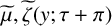. The consequence is that both left- and right-propagating waves with the same growth rate are possible. The upshot is that the range for $\mu _i$ can be confined to the interval $0\leq \mu _i\leq 1/2$ .

To solve the problem (2.3a), the variables are written in harmonics

$$ \begin{align*}(\psi,\zeta)= \sum_{n=-\infty}^{\infty}(\psi_n(y),\zeta_n(y))\exp(in\tau).\end{align*} $$

Equating the coefficients of the harmonics within equations (2.3a) and (2.3b) leads to the system of coupled equations

$$ \begin{align*} \bigg(\frac{d^2}{dy^2}-a^2-2\mu-2in\bigg)\zeta_n &= iaR[ \{\zeta_{n-1}-2i\psi_{n-1} \} \mathrm{e}^{-(1+i)y} + \{\zeta_{n+1}+2i\psi_{n+1} \}\mathrm{e}^{-(1-i)y} ]\end{align*} $$

and

$$ \begin{align*} \bigg(\frac{d^2}{dy^2}-a^2\bigg)\psi_n&=\zeta_n. \end{align*} $$

It was noted by Seminara and Hall [Reference Seminara and Hall33] and Hall [Reference Hall20] that a semi-analytical solution of this problem is feasible. It may be shown that it is possible to write

(2.4a) $$ \begin{align} \psi_n=\sum_{k=-\infty}^{\infty}&\bigg\{ \alpha_k \sum_{j=0}^{\infty}A_{jkn} E_{jkn}(\gamma_k)+\beta_k \sum_{j=0}^{\infty}B_{jkn} E_{jkn}(a)\bigg\}\,;\end{align} $$

here the constants

(2.4b) $$ \begin{align}\gamma_k := & \sqrt{a^2+2\mu+2ik}\end{align} $$

and the exponential functions are defined by

(2.4c) $$ \begin{align}E_{jkn}(\bullet):= &\exp\{ -[ \bullet -i(k-n) +|k-n| +2j] y\}, \end{align} $$

while the $\alpha _k$ and $\beta _k$ remain arbitrary for the moment. Finally, we note that the coefficients $A_{jkn}$ and $B_{jkn}$ satisfy rather complicated recurrence relations. In the interests of brevity, we do not set out these relations here and the interested reader could consult [Reference Blennerhassett and Bassom5] or [Reference Hall20] for full details. Now, provided that the real part of each $\gamma _k$ is positive, the far-field $y\to \infty $ elements of the boundary conditions (2.3c) are automatically satisfied. Thus, we only need to ensure that the wall conditions $\psi =~\psi _y=~0$ 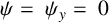hold, which means that

(2.5a) $$ \begin{align} &\sum_{k=-\infty}^{\infty}\bigg\{ \alpha_k \sum_{j=0}^{\infty}A_{jkn} +\beta_k \sum_{j=0}^{\infty}B_{jkn}\bigg\}=0 \end{align} $$

and

(2.5b) $$ \begin{align}\sum_{k=-\infty}^\infty &\bigg\{ \alpha_k\sum_{j=0}^\infty A_{jkn}[ \gamma_k-i(k-n)+|k-n|+2j] \nonumber\\ &\qquad +\beta_k\sum_{j=0}^\infty B_{jkn}[ a-i(k-n)+|k-n|+2j]\bigg\}=0. \end{align} $$

The infinite-dimensional system of equations (2.5a) can be cast as

(2.6) $$ \begin{align} \mathbf{M}\,\mathbf{v} =\mathbf{0}, \end{align} $$

where $\mathbf {v}$ is a column vector consisting of the elements $\{\alpha _k,\beta _k\}$ with $-\infty <k<\infty $ . A nontrivial solution for the vector v is required so that the determinant of the matrix M must vanish. This should yield the form of $\mu $ as a function of $a$ and $R$ .

3 The structure of the neutral curve

A numerical solution to the problem requires a good approximation to the full infinite-dimensional system (2.6). This was done by noting that since the $\psi _n(y)$ are the Fourier coefficients of a smooth periodic function, we expect that they rapidly tend to zero as $n\to \infty $ . Accordingly, we truncate the system and assume that $\psi _m\equiv 0$ for $|m|\geq N+1$ . This leaves a system of $4N+2$ equations for the unknowns $\alpha _r,\beta _s$ for $|r|,|s|\leq N$ . Of course, it needs to be checked that $N$ is chosen to be sufficiently large that the functions $\psi _m$ with $|m|\geq N+1$ are so small that the partial sum represents a sufficiently accurate approximation to the solution of the full system.

Hall [Reference Hall20] tackled this problem, but he could only find stable solutions ( $\mu _r<0$ ) for $R$ up to about 160 and a truncation level of $N=14$ . It turns out that the required size of $N$ tends to increase as $R$ grows and the computer resources available at the time prevented Hall from taking his calculations to any greater $R$ . It was only about a quarter of a century later that Blennerhassett and Bassom [Reference Blennerhassett and Bassom5] revisited this problem. The intervening period of advances in technology, combined with the implementation of some judicious numerical strategies (see [Reference Blennerhassett and Bassom5] for details), enabled the calculations of Hall to be extended to much higher values of $R$ . Indeed, it proved possible to locate a portion of the neutral curve, with growing modes identified once $R$ exceeds about 708. We describe these results below, but note here that the calculations typically required $N$ to be at least 200, and sometimes more than that. This then requires that the zeros of an $800\times 800$ determinant be located and special measures had to be taken to ensure numerical accuracy was preserved.

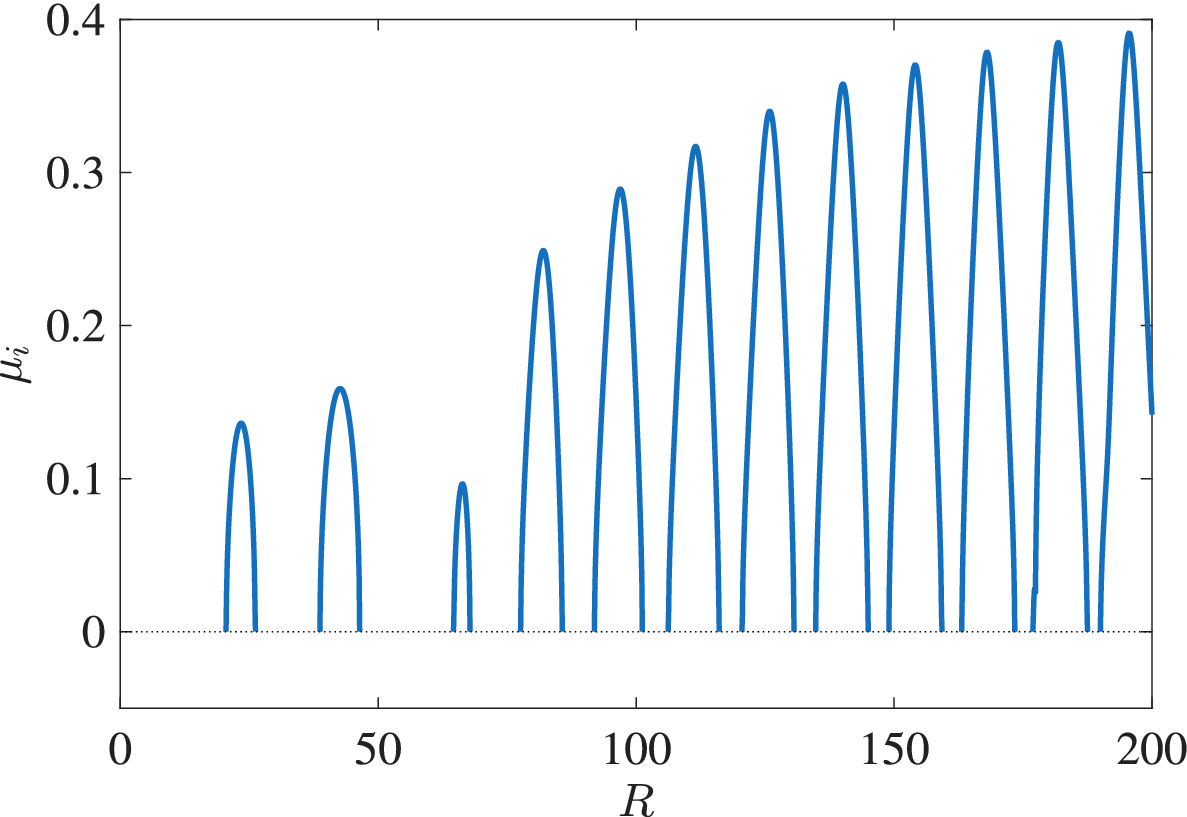
The variation of the imaginary part $\mu _i$ as a function of $R$ up to about 200 and with a wave number $a =0.3$ is shown in Figure 1. There are intervals of $R$ where solutions exist; between these are regions across which no solutions appear to be possible. At the edges of these intervals $\mu _i\to 0$ and $\gamma _0$ is purely imaginary since $a^2+2\mu _r<0$ 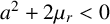. Then the solution is only bounded at infinity rather than decaying in that limit. If these breaks in the solution branches are referred to as S-gaps, it appears that as $R$ increases, the lengths of these gaps decrease. At the same time, the heights of the peaks in Figure 1 appear to grow towards the value 0.5. When $\mu _i\not =0$ , discrete eigenvalues correspond to travelling wave disturbances and, as will be explained presently, the S-gaps eventually evolve into standing wave modes.

Figure 1

The imaginary part $\mu _i$ as a function of $R$ for $a=0.3$ and $R\leq 200$ . The intervals between the solution branches are the S-gaps where there are no solutions that decay as $y\to \infty $ .

Figure 1 Long description

The horizontal axis is labeled R and ranges from 0 to 200 with major ticks every 50 units. The vertical axis is labeled mu sub i and ranges from 0 to 0.4 with major ticks every 0.1 units. A horizontal dotted line is positioned at mu sub i equals 0. The data consists of a series of blue parabolic arches that rise from and return to the zero line.

Moving from left to right along the R axis

* The first arch appears between R equals 20 and 25, peaking at approximately 0.14.

* The second arch is wider, appearing between R equals 35 and 45, peaking at approximately 0.16.

* A large gap exists between R equals 45 and 65.

* A small, narrow arch appears at R equals 65, peaking below 0.1.

* Starting at R equals 75, a series of eleven more arches appear with increasing frequency and height.

* The peaks of these subsequent arches follow a positive linear trend, starting at approximately 0.25 at R equals 80 and reaching nearly 0.4 by R equals 195.

* The intervals of zero value between these arches are identified as S-gaps.

When $a=0.3$ , the results suggest that the disturbance becomes neutrally stable, with $\mu _r=0$ and $\mu _i\not =0$ when $R\approx 780$ . As a consequence, there is a range of $R$ just below this neutral point where $a^2 +2\mu _r$ is positive, and this has an important implication for the nature of the solutions in the S-gaps just below any such neutral points. (With $a=0.3$ , the relevant range is $772\lesssim R\lesssim 780$ .) The behaviour of the eigensolution at infinity is dictated by the nature of the $E_{000}(\gamma _0)$ term in (2.4c). At the edges of the S-gaps $\mu _i=0$ but now, since $a^2 +2 \mu _r> 0$ 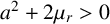, solutions with a negative real part of $\gamma _0$ are possible. Hence, an eigenfunction that decays at infinity exists with $\mu _i = 0$ ; that is, it is a standing wave. We conclude that S-gaps at values $R$ well below neutral conditions contain a continuous spectrum of standing wave modes which do not decay at infinity, since $\gamma _0$ is purely imaginary. By way of contrast, within S-gaps just below neutral conditions, there are discrete, standing wave disturbances that decay from the oscillating plate.

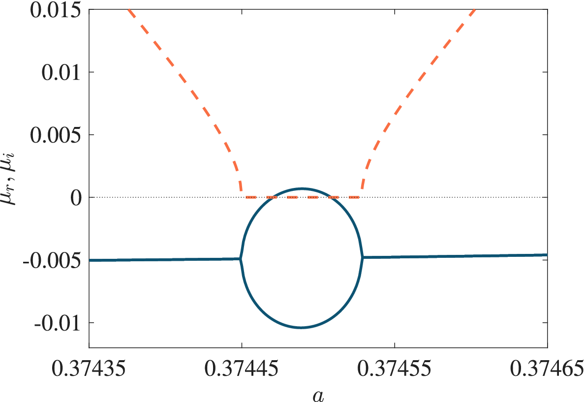
Some greater detail of the above structure is provided in Figure 2 for $R=708$ . Across the S-gap $\mu _i=0$ but is nonzero on either side. Note that where $\mu $ is complex, only the eigenvalues with $\mu _i>0$ have been plotted; the complex conjugate eigenvalues $\widetilde \mu $ have been omitted, so the behaviour of the growth rate can be seen more easily. The endpoints of these intervals clearly correspond to a coalescence of the left and right travelling wave modes, that is, a coming together of complex conjugate eigenvalues, and while $\mu _r$ is a continuous function of $a$ , it must have square-root behaviour at the endpoints of the $\mu _i=0$ interval. The most remarkable feature of the disturbance in this interval is that the two standing wave solutions, coming from the collision of the complex conjugate eigenvalues, have distinctly different growth rates. One of the modes is actually unstable on part of this S-gap. At the upper end of this interval, the standing wave modes are again both stable and they combine to give stable travelling wave modes as $a$ is increased past the right-hand end of the S-gap. The existence of these regions of unstable stationary modes, just below the bulk of the unstable region of parameter space, made the precise determination of the neutral curve far from straightforward.

Figure 2

The real ( $\mu _r$ ; solid) and imaginary ( $\mu _i$ ; dashed) parts of the Floquet exponent $\mu $ as a function of $a$ when $R=708$ . In the left and right portions of the range, where $\mu _i\not = 0$ , the two travelling waves have identical growth rates $\mu _r\, (<0)$ . Across the middle section, where we have coalescence of the travelling waves, $\mu _i\equiv 0$ and the two standing waves have different growth rates. We also see that for a small range of $a$ , one of these standing waves has $\mu _r>0$ so is unstable.

Figure 2 Long description

The horizontal x-axis is labeled a, ranging from 0.37435 to 0.37465. The vertical y-axis is labeled mu sub r, mu sub i, ranging from -0.01 to 0.015. A horizontal dotted line marks the zero baseline.

Two distinct line types represent the data:

1. The imaginary part mu sub i is shown as a dashed orange line. It starts at the top left, descends to zero at a is approximately 0.37445, remains at zero across the middle section, and then ascends symmetrically toward the top right starting at a is approximately 0.37453.

2. The real part mu sub r is shown as a solid blue line. It begins as a single horizontal line at approximately -0.005. At a is approximately 0.37445, it splits into a circular bubble shape. The top half of this bubble crosses the zero baseline into positive values, peaking at approximately 0.001, while the bottom half curves down to -0.01. The two branches recombine at a is approximately 0.37453, returning to a single horizontal line at -0.005 for the remainder of the range.

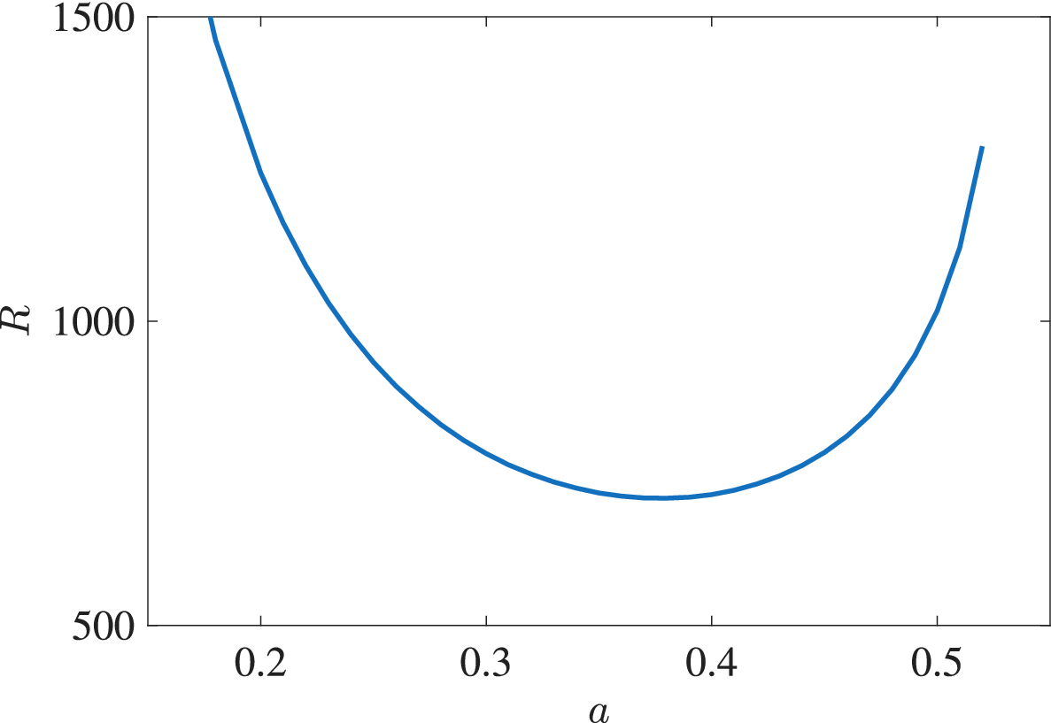
Part of the neutral curve on which $\mu _r=0$ is depicted in Figure 3. This curve was constructed by simple interpolation through neutral points separated in the wave-number domain by an increment of $\Delta a=0.01$ . However, the detailed structure of the curve is rather more intricate than is perhaps suggested by Figure 3. We have just noted that throughout the parameter space, there are short intervals where stationary modes exist with significantly different growth rates. What can happen is that if an interval of stationary modes lies below, but close to the smooth curve in Figure 3, then it is possible for one of the stationary modes to actually become unstable. The complete neutral curve can then only be ascertained by combining the form of the smooth neutral curve with the topology of the regions where stationary modes have $\mu _r=0$ .

Figure 3

Smoothed neutral curve for linear instability in the ( $a,R$ )-plane. Modes in the parameter regime above the curve are linearly unstable.

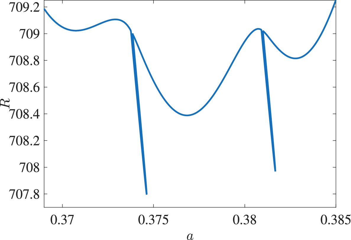
The rather intricate composite curve near the wave number $a=0.38$ is illustrated in Figure 4. The wavy upper section of the curve is a zoomed-in version of the global curve shown in Figure 3. On this section of the curve, the modes take the form of travelling waves with $\mu _i\not =0$ . However, we can see that the upper section is punctured by two thin “fingers”; these are stationary modes with $\mu _i=0$ . We can see that the critical disturbance (that is, the one that occurs at the smallest value $R=R_c$ ) is actually stationary; it has wave number $a\approx 0.3746$ with $R_c\approx 707.84$ . It should be noted that, for this particular value of $a$ , the stationary mode occurs at a lower $R$ than does the corresponding travelling form. However, this only occurs occasionally and, for most wave numbers, it is the travelling mode that is the first to become unstable. The fingers seem to have a length of about $1$ in $R$ -space, so are relatively short. It should also be emphasized that the finger-like structures shown near the minimum of the critical curve in Figure 4 are not restricted to this part of the curve. Strictly speaking, the smoothed form of the curve sketched in Figure 3 should be modified by stationary mode spikes that occur intermittently along the whole line. Significantly, these features are closely connected to the underlying nature of the instability and its spatio-temporal development, which we discuss further in Section 5.

Figure 4

Detailed form of the neutral curve over the range $0.368\leq a\leq 0.385$ .

Figure 4 Long description

A line graph where the horizontal X-axis is labeled ‘a’ and ranges from 0.368 to 0.385. The vertical Y-axis is labeled ‘R’ and ranges from 707.8 to 709.2. The data is represented by a blue curve that exhibits an oscillatory behavior with several peaks and troughs.

Starting from the left at a equals 0.368, the curve begins at R approximately 709.2 and descends to a local minimum near a equals 0.371. It then rises to a local maximum near a equals 0.373. At approximately a equals 0.374, there is a sharp vertical discontinuity where the curve drops abruptly from R equals 709 to R equals 707.8.

Following this drop, the curve rises again to form a broad U-shaped trough with a minimum at a equals 0.377 and R equals 708.4. It ascends to another local maximum at a equals 0.381. Immediately after this peak, a second sharp vertical discontinuity occurs, dropping the value from R equals 709 to approximately 708.

The final segment of the curve rises from this drop into a shallow trough centered at a equals 0.383 and ends with a steep upward trend reaching R equals 709.2 at the rightmost edge of the graph.

We mentioned in the introduction that the associated experimental investigations have suggested that $R_c\approx 275$ , which is considerably lower than the theoretical prediction based on Floquet theory. Several explanations might account for this discrepancy. One possibility is that although the curve sketched in Figures 3 and 4 constitutes one solution, there may be other neutral curves located elsewhere in the parameter space; however, extensive explorations by [Reference Blennerhassett and Bassom5] failed to detect any. We also point out that experiments are necessarily conducted within a finite apparatus, in contrast to the infinite plane layer used in the theoretical analysis.

This latter point prompted [Reference Blennerhassett and Bassom6] to investigate the stability of oscillatory flow in a finite channel. The flow configuration consists of two parallel plates separated by a distance $2d$ that oscillate synchronously with velocity $U_0\cos \omega t$ . If the dimensionless half-width of the channel is $h$ , the modified form of the basic Stokes flow becomes

$$ \begin{align*} U_B(y,\tau)=\Re\bigg\{ \frac{\cosh((1+i)y)}{\cosh((1+i))h)}\exp(i\tau) \bigg\}\equiv u_1(y)\exp(i\tau)+u_{-1}(y)\exp(-i\tau), \end{align*} $$

for $|y|\leq h$ . The perturbation equations are again given by system (2.3a), albeit with the modified form of $U_B$ and with the boundary conditions given by $\psi =\psi _y=0$ when $y=\pm h$ .

Once the perturbation equations apply over a finite domain, rather than on the semi-infinite region, the semi-analytical solution proposed in [Reference Hall20] is no longer available. Consequently, the calculations performed in [Reference Blennerhassett and Bassom6] were based on pseudo-spectral techniques as derived and described by Fornberg [Reference Fornberg18] or Trefethen [Reference Trefethen44]. The computations revealed that now two families of solutions were feasible. The first, which we will refer to as a wall mode, is concentrated near one of the oscillating walls and is the natural counterpart of the disturbance within a semi-infinite layer. However, the finite geometry also introduces a second structure centred around the middle of the channel; this structure has no counterpart within the semi-infinite layer. Thorough investigations showed that these centre modes are always stable for all values of $a$ and $R$ , so can be safely ignored for the purposes of identifying when the underlying flow becomes unstable.

Blennerhassett and Bassom [Reference Blennerhassett and Bassom6] could therefore focus on the wall modes and they monitored their properties as the channel width varied. As would be expected, when the channel is very wide, with $h\gtrapprox 16$ , the stability characteristics are essentially identical to those of the semi-infinite layer with $R_c\approx 708$ . As $h$ is reduced, the value of $R_c$ falls and appears to attain a minimum when $h\approx 5$ , for which $R_c\approx 645$ . While this is lower than the prediction for the semi-infinite problem, there remains a sizeable discrepancy with the experimental determinations of $R_c$ . In an attempt to more faithfully replicate the practical apparatus, Blennerhassett and Bassom [Reference Blennerhassett and Bassom6] extended their methods to account for perturbations to the Stokes layer that is established within a pipe oscillating along its axis. This basic flow can be expressed in terms of Bessel functions of order zero and the governing system for the disturbance needs to be adapted to properly account for the cylindrical geometry. The critical Reynolds number for pipe flow tends to be smaller than their counterparts for the channel case, but the smallest critical value was still almost twice the experimentally reported result.

The veracity of these various theoretical results based on Floquet theory has naturally been questioned, given the disparity with the carefully conducted experiments. In order to throw more light on this issue, Thomas et al. [Reference Thomas, Bassom, Blennerhassett and Davies38] conducted a series of direct numerical simulations based upon a velocity–vorticity formulation of the governing equations. This enabled the time evolution of disturbances to be tracked in an efficient way. In particular, it proved possible to locate the neutral stability curve for two-dimensional disturbances and this was found to be in excellent agreement with the outcomes of the Floquet studies. As a by-product, the two-dimensional neutral stability results were then used to validate the extension of the direct numerical solution code to describe three-dimensional disturbances that take the form of oblique waves.

The methods introduced in [Reference Thomas, Bassom, Blennerhassett and Davies38] were subsequently adapted in [Reference Thomas, Bassom, Blennerhassett and Davies39] to look at the stability of oscillatory Poiseuille flow in both channels and pipes. In these calculations, the underlying basic motion consists of a steady pressure-gradient-driven velocity field coupled with a purely oscillatory component generated either using an oscillatory pressure gradient or by harmonically oscillating the bounding surfaces. Both plane channel and circular pipe geometries were studied and neutral stability curves and critical conditions for instability computed for a selection of steady–unsteady velocity ratios, channel half-widths and pipe radii. The results obtained again confirm previous investigations into the effects of small amounts of periodic modulation on the linear stability of the underlying steady flow, but provided much more comprehensive information on the linear stability regions of unsteady parallel flows in channels and pipes.

These numerical methods were extended by [Reference Thomas, Bassom and Blennerhassett37] to probe the three-dimensional linear stability of the Stokes layer generated within a fluid contained inside a long oscillating cylinder. Critical parameters for instability were obtained for an extensive range of pipe radii and longitudinal and azimuthal wave numbers. We noted earlier that Squire’s theorem holds for an infinite plane Stokes layer, but the results established in [Reference Thomas, Bassom and Blennerhassett37] show that, for sufficiently small pipe diameters, three-dimensional perturbations are actually more unstable than their two-dimensional counterparts. By way of contrast, at larger radii, the three-dimensional disturbance modes are less important and the two-dimensional versions are dominant, so are expected to be observed in practice. These results have important implications for the constraints that should be imposed on experiments that are designed to exhibit shear modes in oscillatory flow.

4 The discrepancy between theory and experiment: a plausible explanation?

Thus far, we have seen that there remains a rather large difference in the critical conditions predicted by Floquet theory and those measured in the laboratory. In their calculations, Blennerhassett and Bassom [Reference Blennerhassett and Bassom5] had noted that a neutral disturbance mode, though periodic over the course of one complete period $0\leq \tau \leq 2\pi $ , undergoes intervals of rapid growth (together with corresponding times of rapid decay). If we adopt the magnitude of the wall vorticity $\zeta _{\mathrm {w}}:= |\zeta (0,\tau )|$ as an avatar for the size of the disturbance, then over the course of a cycle and with $R=255$ (close to experimental conditions) the greatest value of $\zeta _{\mathrm {w}}$ is about ten times its least. Once $R=500$ this ratio becomes 40, and near the theoretical critical $R=708$ it is almost 200. The implication is that if we allow for a maximum disturbance amplitude of 2% at critical conditions, the background noise in the wall vorticity would need to be less than about 0.01% if the predicted linear stability were to be observable experimentally. This requirement is unrealistically demanding; typical equipment, such as that described by Eckmann and Grotberg [Reference Eckmann and Grotberg17], reports noise levels of maybe a few per cent at best.

In an effort to assess the effect of noise on the stability of the plane Stokes layer, Thomas et al. [Reference Thomas, Blennerhassett, Bassom and Davies41] examined a generalisation of the problem of a Stokes layer between a pair of infinite flat plates separated by a dimensionless distance $2h$ . As a paradigm for wall noise, the plate velocities $U_w$ were set to be

(4.1) $$ \begin{align} U_w=U_0\cos\tau+U_0\delta( \alpha_p\cos p\tau+\beta_p\sin p\tau) \quad\mathrm{where}\ \alpha_p^2+\beta_p^2=1; \end{align} $$

here it has been supposed that the theoretical wall velocity $\cos \tau $ is perturbed by a second frequency $p$ . This effect may be interpreted as a component of noise. The size of this noise is measured by $\delta $ , while its phase relative to the main oscillation is controlled by adjusting $\alpha _p$ and $\beta _p$ as appropriate. Of course, in practical settings, the noise would be expected to comprise a spectrum of frequencies, but for simplicity this model includes just one. The numerical calculations were conducted for noise levels up to about 3%.

With the wall velocity as specified by (4.1), the scaled basic velocity profile is given by

$$ \begin{align*} U_{Bn}(y,\tau)=\Re\,\bigg\{ \frac{\cosh((1+i)y)}{\cosh((1+i)h)}\exp(i\tau) +\delta\frac{\cosh((1+i)y\sqrt{p})}{\cosh((1+i)h\sqrt{p})}(\alpha_p-i\beta_p) \exp(ip\tau) \bigg\}\,. \end{align*} $$

With this basic profile, the governing equation for the perturbation stream function $\psi $ becomes

$$ \begin{align*} \frac{\partial}{\partial\tau}{\mathcal{L}}\psi= \bigg\{ \frac12{\mathcal{L}} -\mu-iaRU_{Bn} \bigg\} {\mathcal{L}}\psi +iaR\bigg(\frac{\partial^2U_{Bn}}{\partial y^2}\bigg) \psi\,; \end{align*} $$

here we have introduced the linear operator

$$ \begin{align*}{\mathcal{L}}\equiv \frac{\partial^2}{\partial y^2}-a^2 \end{align*} $$

and seek solutions with

$$ \begin{align*}\psi=\psi'=0\quad\textrm{on } y=\pm h.\end{align*} $$

Numerical solutions were generated by using a velocity–vorticity formulation based on the strategy proposed by Davies and Carpenter [Reference Davies and Carpenter14].

It is far from clear at the outset which values of the frequency $p$ might prove to be significant. To ascertain the most likely candidates, a sensitivity analysis was conducted. This was done by linearising the problem in $\delta $ , whereupon we suppose that if

$$ \begin{align*}\psi(y,\tau)=\psi^{(0)}(y,\tau)+\delta \psi^{(1)}(y,\tau)+\cdots ,\end{align*} $$

then the corresponding Floquet exponent $\mu =\mu ^{(0)}+ \delta \mu ^{(1)}+\cdots $ . The problem for $\psi ^{(0)}$ replicates the eigenvalue problem solved in [Reference Blennerhassett and Bassom6] and then the governing problem for $\psi ^{(1)}$ is just a forced version of that for $\psi ^{(0)}$ . This can only admit a solution if a suitable solvability condition is satisfied, a constraint that can be derived using standard techniques based on the consideration of appropriate adjoint functions.

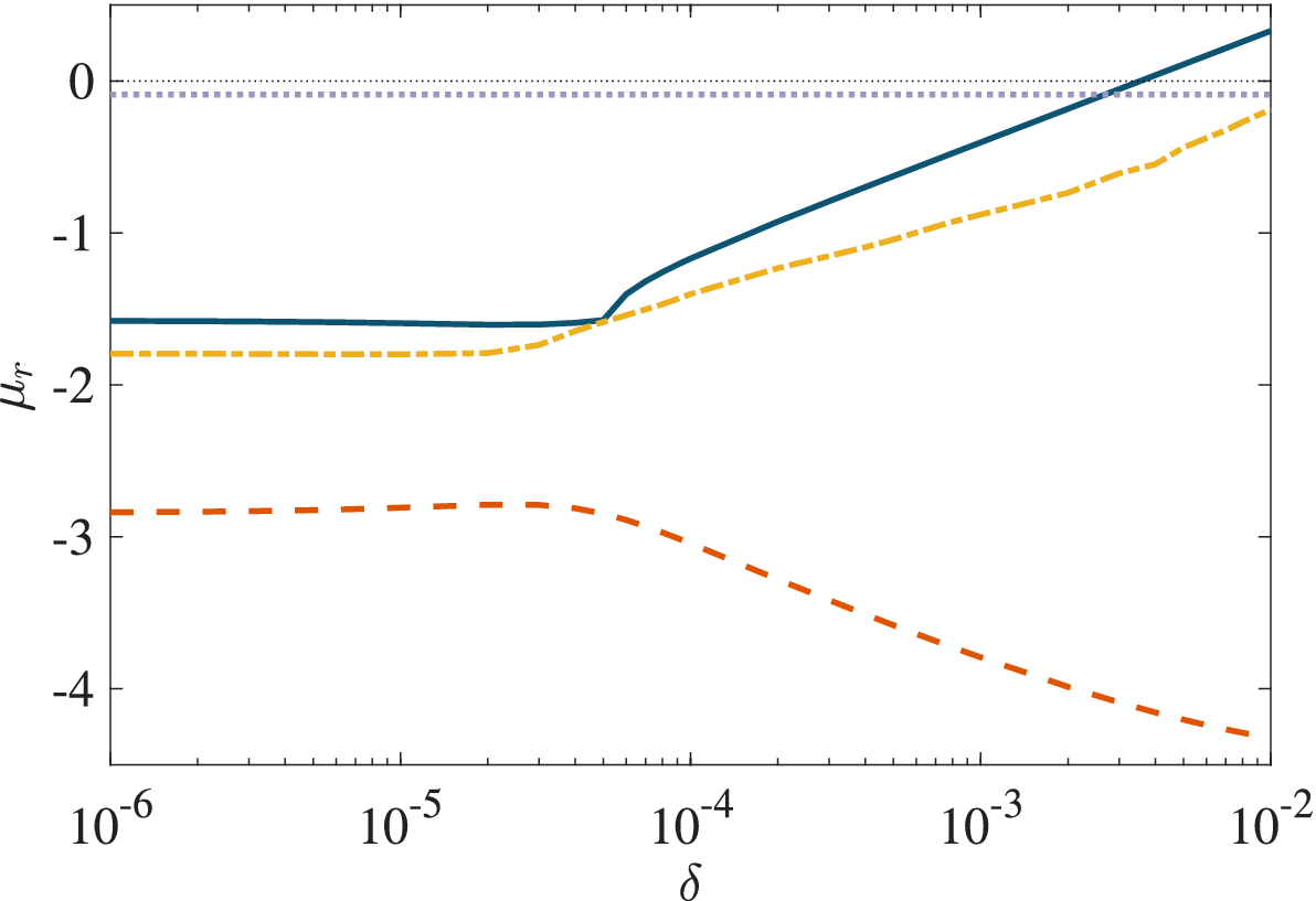
The outcome of this sensitivity analysis yielded the somewhat unexpected result that components of relatively high-frequency noise with $p$ around 50–80 are those that have the most effect on the value of $\mu $ . This informed a subsequent set of calculations for finite $\delta $ . Some representative results are shown in Figure 5, where we illustrate the effect of increasing the size of $\delta $ on the real part of the growth rate $\mu _r$ for both the wall and the centre modes in channels of width 5 and 16 at a Reynolds number $R=300$ . In the narrower channel, the wall mode is always more unstable than the centre mode; moreover, a noise level of a mere 1% is sufficient to make the previously stable flow unstable. This can be deduced from Figure 5 where the blue line is seen to cross over into the unstable $\mu _r>0$ region when $\delta \approx 2\times 10^{-3}$ . We emphasize that this small noise component is enough to drive the transition value of $R$ to less than half its theoretical value for the basic flow in the absence of noise. We also comment that although a 1% noise level is insufficient to make the wide channel unstable, the decay rate of the wall mode is very close to zero, having more than halved.

Figure 5

The real part of the Floquet exponent $\mu _r$ for the wall and centre modes when $R=300$ as the noise level $\delta $ is increased. The solid and dashed lines show the results for the wall mode and centre mode, respectively, for the narrow channel $h=5$ ; the wave number $a=0.41$ and the noise frequency $p=75$ . The chain and dotted lines are the wide channel $h=16$ counterparts with $a=0.38$ and $p=65$ .

Figure 5 Long description

The x-axis represents the noise level delta on a logarithmic scale ranging from 10 super minus 6 to 10 super minus 2. The y-axis represents mu sub r ranging from minus 4 to 0.

* A solid dark blue line (wall mode, h=5) starts at mu sub r approximately minus 1.6, remains flat until delta equals 4 times 10 super minus 5, then increases linearly on the log scale, crossing the zero line at delta approximately 3 times 10 super minus 3.

* A dotted purple line (centre mode, h=16) remains constant and horizontal just below the zero mark at mu sub r approximately minus 0.1 across the entire delta range.

* A dashed yellow line (centre mode, h=5) starts at mu sub r approximately minus 1.8, remains flat until delta equals 4 times 10 super minus 5, then increases linearly, ending near mu sub r minus 0.2.

* A dashed orange line (wall mode, h=16) starts at mu sub r approximately minus 2.8, remains flat until delta equals 4 times 10 super minus 5, then decreases steadily, ending at mu sub r approximately minus 4.3.

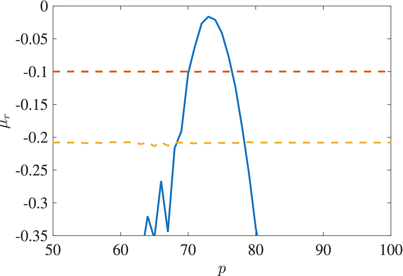
Another perspective on the role of relatively high-frequency noise is provided in Figure 6. Here we illustrate the real part $\mu _r$ for a wave number $a=0.41$ in a wide channel $h=16$ with $R=300$ . We remark that the noise amplitude is fixed at 1% ( $\delta =0.01$ ) and the frequency range $50\leq p\leq 100$ is considered. For $p$ below 50, or above about 85, the eigenvalues obtained are essentially those that would be found for a noise-free, purely oscillatory flow and the results for the wall mode are not visible within the range of $\mu _r$ shown in the figure. Once $p$ is above approximately 60, the wall mode begins to be substantially affected by the noise within the basic flow; $\mu _r$ starts to increase. The wall mode becomes more unstable than both the centre modes for $71\leq p \leq 76$ while, as seen previously, the centre mode eigenvalues remain almost completely unaffected. Again, $\mu $ for the wall mode does not quite reach the right-hand half of the complex plane; it seen in Figure 6 that although the real part of $\mu $ stays negative, it attains a maximum value of about $-0.02$ when $p=73$ , which suggests that the flow is then only very weakly stable.

Figure 6

The real part of $\mu $ for the three most unstable modes as a function of noise frequency $p$ when $h=16, a=0.41, \delta =0.01$ and $R=300$ . The dashed and dotted lines correspond to the first two centre mode disturbances, while the solid line indicates the growth rate of the wall mode.

Figure 6 Long description

The line graph uses a horizontal x-axis labeled p, ranging from 50 to 100, and a vertical y-axis labeled mu sub r, ranging from negative 0.35 to 0.

* A solid blue line representing the wall mode growth rate starts with jagged oscillations below negative 0.35 between p equals 60 and 70. It then rises sharply to a peak of approximately negative 0.02 at p equals 73, before descending steeply back below negative 0.35 by p equals 80.

* A dashed orange horizontal line representing the first centre mode disturbance remains constant at mu sub r equals negative 0.1 across the entire p range.

* A dotted yellow horizontal line representing the second centre mode disturbance remains constant at mu sub r equals negative 0.21 across the entire p range.

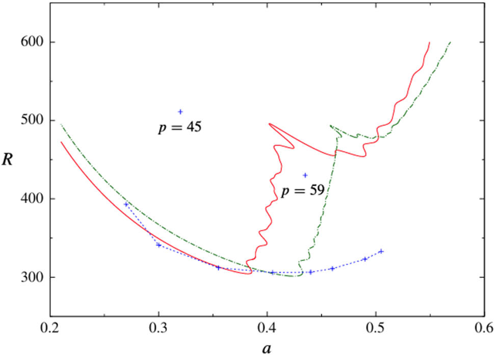
A global view of the effect of noise on the stability of the underlying oscillatory flow is provided by examining suitable neutral stability curves in the $(a,R)$ -plane. Some examples of the neutral stability curves for the noisy flow are shown in Figure 7. Three curves for the most unstable even mode disturbances are illustrated. Despite the slightly unusual shape of these neutral curves, the remarkable feature common to all of them is the surprisingly small value of the critical $R=R_c$ . For the wide channel $h=16$ , the model of the semi-infinite Stokes layer, we see $R_c\approx 305$ for noise frequencies of both 69 and 76. This is a reduction of over 400 compared with its theoretical value of $R_c\approx 708$ for the single-frequency flow. We also note that while the neutral curves drawn in Figure 7 are explicitly for disturbances that exhibit even symmetry about the centre of the channel, the neutral curves for odd modes are graphically indistinguishable.

Figure 7

The neutral curves for a wide channel $h=16$ and noise frequencies $p=69$ (solid curve) and $p=~76$ (dot-dashed curve) with amplitude $\delta =0.01$ . The points denoted by $+$ indicate critical conditions when the perturbation has frequency $p$ as labelled on the graph. The dotted line connects the critical conditions for frequencies $p=61, 63, 67, 79, 85, 91, 95$ and 105 reading from left to right.

Figure 7 Long description

A line graph with the horizontal x-axis labeled a, ranging from 0.2 to 0.6, and the vertical y-axis labeled R, ranging from 300 to 600.

* A solid red curve starts at a equals 0.21, R equals 475, descends to a minimum near a equals 0.38, R equals 305, and then rises sharply with a jagged, oscillating pattern to the right, ending near a equals 0.55, R equals 600.

* A green dot-dashed curve follows a similar path, starting slightly higher at a equals 0.21, R equals 500, reaching a minimum near a equals 0.43, R equals 300, and rising with a jagged pattern to end near a equals 0.57, R equals 600.

* A blue dotted line connects several blue plus symbols, forming a shallow U-shape across the bottom of the graph from a equals 0.27 to a equals 0.51.

* Two isolated blue plus symbols are labeled p equals 45 (located at approximately a equals 0.32, R equals 510) and p equals 59 (located at approximately a equals 0.43, R equals 430).

Superimposed on Figure 7 are the critical conditions (marked by $+$ signs) obtained for a range of other frequencies when $\delta =0.01$ . At this noise level, when $p=35$ , the value of $R_c$ is essentially unchanged from its size $R_c\approx 708$ in a noise-free environment. When $p\in [67,81]$ , we find that $R_c$ remains fairly constant at roughly 305. It is also observed that there is a large jump in the critical wave number between $p=59$ and $p=61$ . While these results apply when $\delta =0.01$ , we note that for $\delta =0.03$ the effect of varying the frequency follows a very similar pattern: when $p=49$ we obtain the critical conditions $a=0.42$ and $R_c=370$ , while with $p=75$ we have $a=0.46$ and $R=275$ .

The analysis summarized here has developed a procedure that has proved capable of explaining mathematically the pivotal role that a small element of high-frequency noise can play in determining the stability of oscillatory flow in a channel. While this can be seen theoretically, there is no obvious physical explanation that we can offer for how this could have been anticipated. There have been various attempts made to rationalize the wide discrepancy between the theoretical and experimentally determined values of the transition Reynolds number. Some arguments appeal to nonlinearity, while others suggest that there might be some premature tripping of the flow by wall roughness. Others have proposed scenarios similar to a bypass-type mechanism that can occur in the transition of steady boundary-layer flows. What is added here is convincing proof that even a small element of noise is more than enough to markedly alter the transition characteristics of the flow. Indeed, our results show that it might only be when the noise is reduced to ${\mathcal {O}}(0.01\%)$ that its effect can be ignored, at least for the Stokes layer. Even the most careful experiments claim that the inherent noise component can only be reduced to a value more than an order of magnitude greater than this.

Up to this stage, we have concentrated on the purely temporal response of a Stokes layer to a disturbance and have asked whether a spatially periodic form amplifies or decays. A related question seeks to understand how a perturbation might evolve both in space and time. We consider this aspect next.

5 Spatio-temporal development

The response of disturbances to the Stokes layer in the spatio-temporal $(x,\tau /2\pi )$ -plane is best studied following the approach of Ramage and his co-workers that has been detailed in [Reference Ramage31, Reference Ramage, Davies, Thomas and Togneri32, Reference Thomas, Davies, Bassom and Blennerhassett42]. The basis of this strategy is founded on the idea that disturbances can be decomposed into Fourier components, incorporating the discrete wave numbers

$$ \begin{align*}a=a_q\equiv q\Delta a \quad \textrm{for } q=0\cdots Q.\end{align*} $$

Since the governing system consists of linear equations, and as the base flow is streamwise homogeneous, the various Fourier components evolve independently of each other. This means that the complete spatio-temporal disturbance generated by a localized impulsive wall forcing can be reconstructed by a simple superposition of all Fourier components. For example, the vorticity perturbation can be written as

$$ \begin{align*} \zeta(x,y,\tau) = \sum_{q=0}^Q\zeta_q(y,\tau)\exp(ia_qx); \end{align*} $$

in this formula we have $x=x_q=q\Delta x$ with $\Delta x \equiv 2\pi /((Q+1)\Delta a)$ . The wave number spacing $\Delta a$ sets the spatial periodicity of the computational domain $2\pi /\Delta a$ , and was chosen sufficiently small so as to ensure the accurate resolution of the form of the disturbance; typically $\Delta a = 2.5\times 10^{-4}$ proved to be adequate for these purposes. Furthermore, the wave number range needs to be wide enough to capture both large- and small-scale behaviours. Practice tests showed that the maximum wave number $a_{\max }= Q\Delta a\approx 0.6$ was adequate. This is somewhat less than might have been anticipated at the outset. However, a larger $a_{\max }$ was not required since wave number components with $a\gtrapprox 0.6$ decay very rapidly indeed.

The governing equations were solved using the numerical scheme developed in [Reference Davies and Carpenter14] based upon a spectral discretisation in the wall-normal $y$ -direction with disturbances expanded in terms of Chebyshev polynomials. The semi-infinite domain $y\in [0,\infty )$ was mapped onto $\xi \in (0,1]$ using the transformation $\xi = s/(y+s)$ ; here the stretching parameter $s$ controls the distribution of points across the Stokes layer. The temporal evolution was computed using an implicit-explicit predictor–corrector scheme. The results described below were obtained using the value $s=4$ , $96$ Chebyshev polynomials and a time step $\Delta \tau = 0.1/R$ which ensures that there are $O(10^4)$ time steps per period of oscillation.

The typical spatio-temporal evolution of an impulsively generated disturbance is shown in Figure 8. The impulse is applied at $x_f=0$ and $R=715$ , which corresponds to a marginally unstable case. Figure 8 depicts contours of the logarithm of the wall-vorticity perturbation amplitude in the $(x,\tau /2\pi )$ -plane. There is clear evidence of the emergence of a family-tree-like structure. Immediately following the initial impulse when $\tau =0$ , a parent wave packet is formed and this propagates downstream in the positive $x$ -direction. During the first period of oscillation, this parent wave packet produces two child wave packets, which are initiated when there is a sign change in the wall shear stress $U_B'$ . One child packet propagates to the right, which corresponds to a negative-to-positive change in $U_B'$ ; the other moves to the left. Each child wave packet subsequently generates two further wave packets over the next period and this process then iterates, thereby generating a repeated branching behaviour that characterizes the formation of a growing family tree.

Figure 8

A spatio-temporal contour plot of the disturbance quantity $\ln |\zeta |$ at the wall. The calculations correspond to $R=715$ and a Stokes layer which is impulsively excited at $x_f=0$ .

Figure 8 Long description

A contour plot with three axes. The horizontal X-axis represents spatial distance x, ranging from -10000 to 10000. The vertical Y-axis represents time tau all over 2 pi, ranging from 0 to 11. A vertical color bar on the right indicates the magnitude of the natural log of the absolute value of zeta, ranging from -10 (dark blue) to 0 (dark red).

At the spatial origin x equals 0 and time tau equals 0, a disturbance originates and propagates outward. The data forms a V-shaped pattern that widens as time increases.

* The core of the disturbance consists of vertical, elongated elliptical structures.

* These structures are most intense (red and orange, values -2 to 0) along the right edge of the V-shape, particularly for positive x values between 0 and 10000.

* The left side of the V-shape (negative x values) shows lower intensity disturbances (cyan and blue, values -6 to -10).

* As time tau all over 2 pi increases from 0 to 11, the spatial extent of the disturbance grows from a single point at x equals 0 to a width spanning nearly the entire x-axis range at the top of the plot.

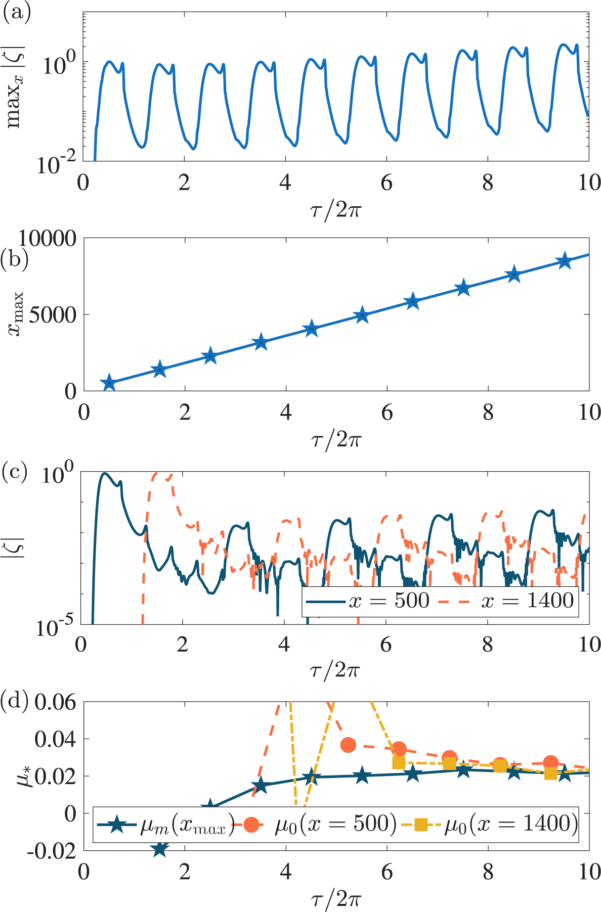
It is clear from Figure 8 that the disturbance maximum convects along the outermost wave packets on the right-hand side of the tree structure. The corresponding temporal evolution of the maximum wall-vorticity amplitude, $\max _x |\zeta |$ , is illustrated in Figure 9(a). From one oscillation period to the next, the disturbance amplitude undergoes a small but sustained increase, which is indicative of the onset of linear instability. An estimate of the growth rate can be derived using the formula

$$ \begin{align*} \mu_m(\tau)=\dfrac{1}{2\pi}\ln\bigg(\dfrac{\max_x|\zeta(x,0,\tau+2\pi)|}{\max_x|\zeta(x,0,\tau)|}\bigg)\,, \end{align*} $$

where $\max _x|\zeta |$ is evaluated at the midpoint of each oscillation cycle. The growth rate, as shown in Figure 9(d), approaches a positive constant as $\tau $ increases, and this is consistent with the Floquet exponent determined in [Reference Blennerhassett and Bassom5]. Increasing the Reynolds number leads to correspondingly larger growth rates and stronger instability.

Figure 9

The disturbance characteristics of the family-tree structure shown in Figure 8. (a) The temporal evolution of the maximum wall-vorticity perturbation amplitude, $\max _x |\zeta |$ . (b) The streamwise location $x_{\max }$ of this maximum measured at the midpoint of each wall cycle (stars). The corresponding line of best fit is shown by the solid line. (c) The temporal evolution of $|\zeta |$ at two locations: $x=500$ (solid) and $x=1400$ (dashed). (d) The growth rate $\mu _m$ of the disturbance maximum in (a) (solid), and pointwise growth rate, $\mu _0$ , at the locations in (c).

Figure 9 Long description

The four panels share a common x-axis representing time as tau all over 2 pi, ranging from 0 to 10.

Panel a: The y-axis is max sub x absolute value zeta on a logarithmic scale from 10 super minus 2 to 10 super 0. The blue line shows a periodic oscillating trend with peaks slightly increasing in magnitude over time.

Panel b: The y-axis is x sub max ranging from 0 to 10000. Blue stars represent data points at the midpoint of each cycle, connected by a solid blue line showing a perfectly linear increase from near 0 at tau all over 2 pi equals 0.5 to approximately 9000 at tau all over 2 pi equals 10.

Panel c: The y-axis is absolute value zeta on a logarithmic scale from 10 super minus 5 to 10 super 0. A solid blue line for x equals 500 shows an initial peak followed by lower-amplitude oscillations. A dashed orange line for x equals 1400 shows a delayed onset, peaking around tau all over 2 pi equals 1.5, then settling into oscillations that are higher in amplitude than the x equals 500 line.

Panel d: The y-axis is mu sub asterisk ranging from minus 0.02 to 0.06. A solid blue line with stars for mu sub m (x sub max) shows a steady increase toward a value of 0.02. Pointwise growth rates mu sub 0 are shown for x equals 500 (orange dashed line with circles) and x equals 1400 (yellow dashed line with squares), both exhibiting high initial fluctuations before converging toward the mu sub m value near 0.02.

The streamwise location of the disturbance maximum $x_{\max }$ is plotted in Figure 9(b). A distinct $\Lambda $ -spacing emerges between successive wave packets and the disturbance maximum propagates a distance $\Lambda \approx 850$ during each oscillation period. It was shown in [Reference Ramage, Davies, Thomas and Togneri32] that the spacing between adjacent wave packets is proportional to the Reynolds number.

The Stokes layer (2.1) is both time-periodic and anti-periodic in the sense that $U_B(y,\tau +2\pi )=U_B(y,\tau )$ and $U_B(y,\tau +\pi )=-U_B(y,\tau )$ . This symmetry structure is reflected in the staggered family-tree disturbance development and its associated temporal response. In particular, the wave-packet formation is approximately symmetric about $x=0$ , except for the outermost packet that contains the disturbance maximum. This symmetry, together with the staggered structure of the packets, leads to a separation of $2\Lambda $ between packets of commensurate size, thereby leading to an overall spatial periodicity of $2\Lambda $ .

The pointwise growth of the disturbance is monitored by fixing a streamwise location and then tracking the temporal development at that location. Figure 9(c) shows the evolution of $|\zeta |$ at the two locations $x=500$ and $x=1400$ . After an initial transient phase, the peak amplitudes occur alternately between oscillation cycles, which reflects the staggered wave-packet formation. Moreover, the disturbance amplitude increases every two oscillation periods, which demonstrates a sub-harmonic temporal growth with periodicity twice that of the basic state. The pointwise growth rate was calculated using

$$ \begin{align*} \mu_0(\tau)=\dfrac{1}{4\pi}\ln\bigg(\dfrac{|\zeta(x,0,\tau+4\pi)|}{|\zeta(x,0,\tau)}\bigg), \end{align*} $$

and the results are illustrated in Figure 9(d). As $\tau $ increases, the pointwise growth rates approach the same positive value associated with the disturbance maximum. This observation is consistent with an instability that exhibits absolutely unstable behaviour. Accordingly, we next consider the form of the absolute instability mechanisms that are responsible for the development of the family-tree structure.

5.1 Absolute instability

Pretty et al. [Reference Pretty, Davies and Thomas29] considered the stability of the Stokes layer using a modified form of the Briggs–Bers [Reference Briggs10] method to distinguish between convectively and absolutely unstable behaviour. Convective instability describes a disturbance that grows while propagating in one direction only, whereas absolute instability is characterized by growth at every spatial location. The approach follows [Reference Brevdo and Bridges9] for temporally oscillating flows, with Floquet theory used to account for the time-periodicity of the base flow. Given the periodicity properties of the Stokes layer, we can derive symmetry constraints that can help classify the type of instability that develops.

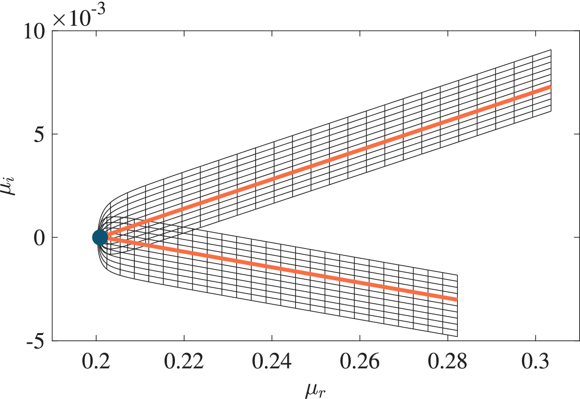
To identify absolute instability, properties were coupled to the cusp-map method [Reference Kupfer, Bers and Ram23] in which the streamwise wave number $\alpha \in \mathbb {C}$ is mapped onto the complex Floquet exponent $\mu $ -plane. Two types of cusps can arise, and these are associated with Floquet exponents $\mu =\mu _r+ik/2$ . If $k=0$ there is harmonic behaviour, whereas $k=1$ corresponds to a sub-harmonic structure. Figure 10 demonstrates a cusp structure when $R=750$ for which $\mu _r=0.2009$ and $\mu _i=0$ . The cusp occurs at a real-valued wave number $\alpha $ and, since $\mu _r>0$ , symmetry arguments imply pointwise growth and therefore absolute instability. This cusp is associated with $\mu _i=0$ and corresponds to the tip of a finger-like protrusion along the neutral stability curve and hence harmonic growth. Analogous cusp structures arise for $\mu _i \approx 1/2$ with $\mu _r>0$ , and these are associated with sub-harmonic growth.

Figure 10

Cusp formation in the complex $\mu $ -plane when $R=750$ . This solution corresponds to $\mu _i=0$ and the tip of a finger protrusion in Figure 11.

Figure 10 Long description

The horizontal X axis is labeled mu sub r and ranges from 0.2 to 0.3. The vertical Y axis is labeled mu sub i and ranges from minus 5 to 10, with a scale factor of 10 super minus 3 at the top left.

At the coordinate (0.2, 0), a large dark blue circular dot serves as the anchor point for a cusp. From this point, a grid-like structure composed of fine black lines expands to the right. The structure splits into two distinct branches:

* The upper branch follows a linear upward trend, centered around a thick orange line that reaches approximately mu sub i equals 7.5 at mu sub r equals 0.3.

* The lower branch follows a linear downward trend, centered around a thick orange line that reaches approximately mu sub i equals minus 3 at mu sub r equals 0.28.

The black grid lines form concentric parabolic curves near the cusp and transition into a rectangular mesh as the branches extend and diverge.

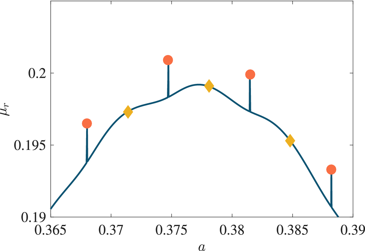
When $R=750$ , several cusps with positive real part $\mu _r>0$ are marked in Figure 11. Four cusps at the tips of fingers ( $\mu _i=0$ ) are shown by the red circular markers and three cusps with $\mu _i \approx 1/2$ are located about the mid-points between adjacent protrusions. The pointwise growth is therefore characterized by a combination of harmonic and sub-harmonic absolutely unstable modes. These features extend to other Reynolds numbers, including the critical value $R_c \approx 707.84$ , where a stationary disturbance first appears along a $\mu _i=0$ finger. This proves that the onset of instability coincides with the onset of absolute instability.

Figure 11

The Floquet growth rate $\mu _r$ as a function of wave number $a$ when $R=750$ . The red circle and yellow diamond markers highlight locations matched to absolutely unstable harmonic ( $\mu _i=0$ ) and sub-harmonic modes ( $\mu _i=1/2$ ), respectively.

Figure 11 Long description

The horizontal X axis represents wave number a, ranging from 0.365 to 0.39. The vertical Y axis represents the Floquet growth rate mu sub r, ranging from 0.19 to 0.2. A dark blue curve rises from the bottom left, peaks near a equals 0.378, and descends toward the bottom right.

Seven specific markers are plotted relative to this curve:

* Red circles represent absolutely unstable harmonic modes where mu sub i equals 0. These are located at a equals 0.368, 0.375, 0.382, and 0.388. Each red circle is positioned above the blue curve and connected to it by a vertical blue line segment.

* Yellow diamonds represent sub-harmonic modes where mu sub i equals 1 divided by 2. These are located at a equals 0.371, 0.378, and 0.385. These markers sit directly on the dark blue curve.

The curve shows a slight undulating behavior rather than a smooth parabola, with the highest growth rate occurring at the central yellow diamond marker.

Further work in this direction by Ramage et al. [Reference Ramage, Davies, Thomas and Togneri32] examined the effect of introducing a high-frequency component of noise into the basic flow. It will be recalled that [Reference Thomas, Blennerhassett, Bassom and Davies41] had previously shown that even a small noise element proportional to $\cos (p\tau )$ is sufficient to significantly reduce the critical Reynolds number for linear instability. For small amplitudes, the disturbance retains the family-tree structure and sub-harmonic growth, but a distinction needs to be drawn on whether $p$ is even or odd. When $p/2\in \mathbb {N}$ , an additional spatial asymmetry arises owing to a breakdown of the anti-periodicity of the oscillatory basic state, since the relation $U_B(y,\tau +\pi )=-U_B(y,\tau )$ no longer holds. The symmetry between positive and negative directions that characterizes the unmodified Stokes layer is then lost. As the amplitude of the high-frequency harmonic is increased, the family-tree formation is gradually modified and eventually becomes a single wave packet that alternates in space between successive cycles. Concurrently, the sub-harmonic behaviour observed in the unmodified Stokes layer is replaced by oscillations at the fundamental period of the modified base state. The overall effect is that absolutely unstable behaviour becomes evident at earlier times than in the canonical Stokes layer.

5.2 Skewed flows

The basic Stokes layer can be extended to include both acceleration and velocity skewness. This introduces asymmetry into the periodic base flow and the resulting profile is thought to be a good model for motions seen in coastal dynamics where wave propagation is characterized by skewness in the wave depth, wave height and wave period. The velocity skewness generates a wave characterized by a narrow, sharp crest together with a broad, flat trough, while acceleration skewness produces wave asymmetry.

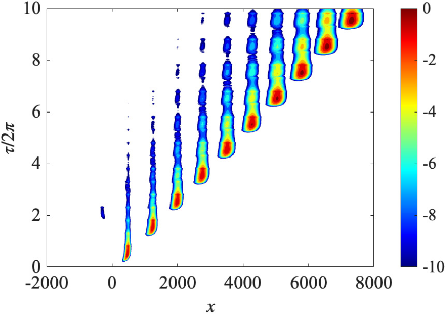
The linear stability of acceleration-skewed and velocity-skewed flows has been investigated in [Reference Thomas35, Reference Thomas36], respectively. Acceleration skewness tends to destabilize the Stokes layer and reduces the critical Reynolds number, while velocity skewness has the opposite effect. Further insight into the effect of skewness on linear instability is provided by the impulse response of disturbances in the spatio-temporal plane, as described in [Reference Thomas and Pretty43]. Figure 12 illustrates the typical behaviour observed in both acceleration-skewed and velocity-skewed flows for conditions matched to linear instability. While the overall structure is similar to the family-tree behaviour observed in the symmetric Stokes layer (see Figure 8), skewness introduces a marked asymmetry in the spatial development. The disturbance maximum again convects along the rightmost branch of the structure, but wave packets propagating to the left decay and ultimately dissipate. The consequence is that the characteristic sub-harmonic growth associated with the Stokes layer is lost. This behaviour arises because acceleration- and velocity-skewed flows are no longer anti-periodic, unlike the classical Stokes layer. As a result, the onset of linear instability in skewed flows corresponds to convective instability rather than the absolute instability observed for the Stokes layer. It is only at a much higher Reynolds number that sub-harmonic growth re-emerges and absolute instability sets in.

Figure 12

A spatio-temporal contour plot of the linear disturbance $\ln |\zeta |$ in an acceleration-skewed Stokes layer. Here $R=635$ and motion is impulsively excited at $x_f=0$ .

Figure 12 Long description

A contour plot with a horizontal x-axis ranging from -2000 to 8000 and a vertical y-axis labeled tau all over 2 pi ranging from 0 to 10. A color bar on the right indicates values from -10 in dark blue to 0 in dark red. The data consists of approximately ten distinct vertical wave packets or contours that propagate diagonally from the bottom-left toward the top-right. The first significant packet appears near x equals 500 and tau all over 2 pi equals 0. Each subsequent packet to the right starts at a higher tau value, creating a stepped diagonal progression. Within each packet, the core is red (highest value near 0) surrounded by concentric layers of yellow, green, and light blue, fading into a dark blue background (lowest value near -10). The packets broaden slightly in the x-direction as they move higher up the y-axis.