1 Introduction
In the past one and a half centuries, the Boltzmann equation has achieved great success in describing the dynamics of rarefied ideal gases, that is, the gas is sufficiently dilute that only binary collisions need to be taken into account (Chapman & Cowling Reference Chapman and Cowling1970). However, if the gas is compressed to the level that the molecular dimensions are comparable to the average distance between neighbouring molecules, the effect of finite molecular size must be considered (Ferziger & Kaper Reference Ferziger and Kaper1972). This is found in many applications, including high-pressure shock tubes (Petersen & Hanson Reference Petersen and Hanson2001), sonoluminescence (Brenner, Hilgenfeldt & Lohse Reference Brenner, Hilgenfeldt and Lohse2002), gas extraction in unconventional reservoirs (Wu et al. Reference Wu, Liu, Reese and Zhang2016; Sander, Pan & Connell Reference Sander, Pan and Connell2017) and the interfacial dynamics of liquid–vapour at supercritical pressures (Dahms et al. Reference Dahms, Manin, Pickett and Oefelein2013; Dahms & Oefelein Reference Dahms and Oefelein2015).
Enskog (Reference Enskog1922) was the first to extend the Boltzmann equation to dense gases of rigid spherical molecules by considering the non-local collisions and the increased collision frequency due to the finite size of the gas molecules (Chapman & Cowling Reference Chapman and Cowling1970; Ferziger & Kaper Reference Ferziger and Kaper1972). Similar to the Boltzmann equation, the Enskog equation can be solved numerically using a probabilistic or deterministic method. The pioneering work of solving the Enskog equation was carried out by Frezzotti & Sgarra (Reference Frezzotti and Sgarra1993) using a Monte Carlo quadrature method, and its accuracy was confirmed by comparison with the molecular dynamics (MD) simulation of the shock wave structure in a dense hard-sphere gas. Subsequently, inspired by the direct simulation Monte Carlo (DSMC) method for the Boltzmann equation, several probabilistic methods were developed by Alexander, Garcia & Alder (Reference Alexander, Garcia and Alder1995), Montanero & Santos (Reference Montanero and Santos1996) and Frezzotti (Reference Frezzotti1997b) to solve the Enskog equation. Recently, a fast spectral method (FSM) method was proposed by Wu, Zhang & Reese (Reference Wu, Zhang and Reese2015) to deterministically solve the generalized Enskog equation, which has spectral accuracy in computing the collision operator at reduced computational cost, and has been successfully applied to study the non-equilibrium dynamics of a dense gas under tight confinement (Wu et al. Reference Wu, Liu, Reese and Zhang2016). More recently, Sadr & Gorji (Reference Sadr and Gorji2017, Reference Sadr and Gorji2019) also developed the Fokker–Planck approximation of the Enskog equation for non-equilibrium dense gases, which was validated by comparison with the results of the Enskog model solved by the Monte Carlo method (Montanero & Santos Reference Montanero and Santos1996).
Although these methods for direct solution of the Enskog equation could provide reliable results, the computational costs are still formidable for practical applications. Therefore, it is beneficial to simplify the Enskog collision operator to achieve efficient computations with reasonable accuracy. The first attempt, although not designed for numerical simulations, was made in the derivation of transport coefficients such as viscosity and thermal conductivity, where the Enskog collision operator was expanded into a Taylor series of molecular diameter. The zeroth-order term gave the Boltzmann collision operator, and in the first-order terms the velocity distribution function (VDF) was approximated by the local equilibrium distribution function, while the other high-order terms were neglected (Chapman & Cowling Reference Chapman and Cowling1970). In developing the lattice Boltzmann model (LBM) for hydrodynamic flows of both liquid and gas, Luo (Reference Luo1998, Reference Luo2000) borrowed and simplified the Enskog equation by replacing the Boltzmann collision operator with a Bhatnagar–Gross–Krook (BGK) collision operator (Bhatnagar, Gross & Krook Reference Bhatnagar, Gross and Krook1954), while maintaining the first-order terms relevant to the density spatial derivative. Later, by including the long-range attractive force, the BGK–Enskog model was used to develop the LBM multiphase model by He & Doolen (Reference He and Doolen2002). However, the above LBM works only considered hydrodynamic flows. As a consequence of the inherent coupling between the discretized molecular velocity and the spatial grid in the standard LBM, the limited number of discrete velocities in LBM results in poor numerical stability, and its simulation is limited to low-speed flow (Guo & Shu Reference Guo and Shu2013). Hence, these LBM models are not appropriate for simulating compressible flows.
Subsequently, Guo, Zhao & Shi (Reference Guo, Zhao and Shi2005, Reference Guo, Zhao and Shi2006) proposed a simplified kinetic model for strongly inhomogeneous confined flow by considering the attractive force among molecules and the wall potential, from which the generalized hydrodynamic equations for fluid flows from the nanoscale to the macroscale were derived based on the Chapman–Enskog expansion. However, Guo et al. (Reference Guo, Zhao and Shi2005, Reference Guo, Zhao and Shi2006) only studied equilibrium flow properties with a no-slip boundary condition, so non-equilibrium effects were not properly considered. Here, we aim to propose an accurate and efficient model equation to describe rarefied flow of dense gases that underpin many technological developments.
In this work, a simplified model of the Enskog equation is to be developed on the basis of the Shakhov model for dense gases of monatomic rigid molecules, which is presented in § 2. In order to test its accuracy, the structure of a normal shock wave in a dense gas is calculated by the proposed model, and the results are compared to the solutions of the Enskog equation using the FSM, which are presented in § 3.
2 The Shakhov–Enskog equation
2.1 The Enskog equation
To describe non-equilibrium (rarefied) flow of dilute gases, the Boltzmann equation assumes that the collisions between molecules occur instantaneously and only two-body interaction exists between molecules. In the time between two collisions, the molecule is only affected by an external force, and its motion is independent of other molecules. The collisions between molecules are statistically independent. When the gases become dense, the space occupied by molecules needs to be considered, and molecular transport cannot be completely described by the free motion between two consecutive collisions.
Enskog (Reference Enskog1922) studied the transport of dense gases comprising rigid, elastic and spherical molecules, and developed the Enskog–Boltzmann equation with the following two arguments. First, when two molecules collide, their positions are not at the same point, but one molecular diameter apart. As binary collisions are assumed in the Enskog equation, it is only applicable for moderately dense gases. Second, the volume occupied by the gas molecules reduces the space of free movement of each molecule, and hence the number of collisions between molecules increases. As a further approximation, the collision operator of the Boltzmann equation can be modified and extended to the Enskog equation for hard-sphere molecules as (Chapman & Cowling Reference Chapman and Cowling1970)
 $$\begin{eqnarray}\frac{\unicode[STIX]{x2202}f}{\unicode[STIX]{x2202}t}+\unicode[STIX]{x1D743}\boldsymbol{\cdot }\unicode[STIX]{x1D735}_{x}\,f+\boldsymbol{a}\boldsymbol{\cdot }\unicode[STIX]{x1D735}_{\unicode[STIX]{x1D709}}\,f=\unicode[STIX]{x1D6FA},\end{eqnarray}$$
where  $f(\boldsymbol{x},\unicode[STIX]{x1D743},t)$ is the VDF of the molecular velocity
 $\unicode[STIX]{x1D743}$ at position
 $\boldsymbol{x}$ and time
 $t$,
 $m\boldsymbol{a}$ is the external body force (
 $m$ is the molecular mass), and
 $\unicode[STIX]{x1D735}_{x}$ and
 $\unicode[STIX]{x1D735}_{\unicode[STIX]{x1D709}}$ are the gradient operator with respect to the physical space and molecular velocity, respectively. On the right-hand side of (2.1),
 $\unicode[STIX]{x1D6FA}$ is the Enskog collision operator with the form
 $$\begin{eqnarray}\unicode[STIX]{x1D6FA}=\unicode[STIX]{x1D70E}^{2}\int \left\{\unicode[STIX]{x1D712}\left(\boldsymbol{x}+\frac{\unicode[STIX]{x1D70E}}{2}\boldsymbol{k}\right)f^{\prime }(\boldsymbol{x})f_{1}^{\prime }(\boldsymbol{x}+\unicode[STIX]{x1D70E}\boldsymbol{k})-\unicode[STIX]{x1D712}\left(\boldsymbol{x}-\frac{\unicode[STIX]{x1D70E}}{2}\boldsymbol{k}\right)f(\boldsymbol{x})f_{1}(\boldsymbol{x}-\unicode[STIX]{x1D70E}\boldsymbol{k})\right\}\boldsymbol{g}\boldsymbol{\cdot }\boldsymbol{k}\,\text{d}\boldsymbol{k}\,\text{d}\unicode[STIX]{x1D743}_{\mathbf{1}}.\end{eqnarray}$$
Here  $\unicode[STIX]{x1D70E}$ is the effective molecular diameter,
 $\boldsymbol{g}=\unicode[STIX]{x1D743}_{1}-\unicode[STIX]{x1D743}$ is the relative velocity of two colliding molecules, and
 $\boldsymbol{k}$ is the unit vector that specifies their relative position at the time of impact. In addition,
 $f^{\prime }(\boldsymbol{x})\equiv f(\boldsymbol{x},\unicode[STIX]{x1D743}^{\prime },t)$,
 $f_{1}^{\prime }(\boldsymbol{x})\equiv f(\boldsymbol{x},\unicode[STIX]{x1D743}_{1}^{\prime },t)$,
 $f_{1}(\boldsymbol{x})\equiv f(\boldsymbol{x},\unicode[STIX]{x1D743}_{1},t)$ and
 $f(\boldsymbol{x})\equiv f(\boldsymbol{x},\unicode[STIX]{x1D743},t)$, where the post-collision velocities
 $\unicode[STIX]{x1D743}^{\prime }$ and
 $\unicode[STIX]{x1D743}_{1}^{\prime }$ are related to the pre-collision molecular velocities
 $\unicode[STIX]{x1D743}$ and
 $\unicode[STIX]{x1D743}_{1}$ through
 $\unicode[STIX]{x1D743}^{\prime }=\unicode[STIX]{x1D743}+\boldsymbol{k}(\boldsymbol{g}\boldsymbol{\cdot }\boldsymbol{k})$ and
 $\unicode[STIX]{x1D743}_{1}^{\prime }=\unicode[STIX]{x1D743}_{1}-\boldsymbol{k}(\boldsymbol{g}\boldsymbol{\cdot }\boldsymbol{k})$.
In comparison with the Boltzmann equation, a radial distribution function (RDF)  $\unicode[STIX]{x1D712}$ is introduced in the Enskog collision operator (2.2) to include the effect of the physical dimensions of the molecules on the intermolecular collision frequency. The RDF depends on the local density
 $\unicode[STIX]{x1D70C}(\boldsymbol{x},t)$ and can be approximated by (Carnahan & Starling Reference Carnahan and Starling1969; Chapman & Cowling Reference Chapman and Cowling1970)
 $$\begin{eqnarray}\unicode[STIX]{x1D712}(\unicode[STIX]{x1D70C})=\frac{1-0.125b\unicode[STIX]{x1D70C}}{(1-0.25b\unicode[STIX]{x1D70C})^{3}}\end{eqnarray}$$
or
 $$\begin{eqnarray}\unicode[STIX]{x1D712}(\unicode[STIX]{x1D70C})=\frac{1-(11/8)b\unicode[STIX]{x1D70C}}{1-2b\unicode[STIX]{x1D70C}}.\end{eqnarray}$$
In (2.3) and (2.4),  $b=2\unicode[STIX]{x03C0}\unicode[STIX]{x1D70E}^{3}/3m$, which relates to the reduced density
 $\unicode[STIX]{x1D702}$ as
 $\unicode[STIX]{x1D702}=b\unicode[STIX]{x1D70C}/4$. Note that (2.4) is only used in this work for consistent comparison with the reported solutions of the Enskog equation obtained by the Monte Carlo method (Frezzotti & Sgarra Reference Frezzotti and Sgarra1993). In comparison with (2.4), the RDF defined by (2.3) agrees extremely well with the MD data given by Alder & Wainwright (Reference Alder and Wainwright1960) up to the phase transition. Therefore, equation (2.3) will be applied for the rest of the simulations. When
 $\unicode[STIX]{x1D70E}$ approaches zero,
 $\unicode[STIX]{x1D712}$ is unity, and the Enskog collision operator (2.2) reduces to that of the Boltzmann equation. It is apparent that direct numerical solution of the Enskog equation (2.1) is even more time-consuming than that of the Boltzmann equation, restricting its practical applications. Therefore, it is important to simplify the Enskog equation to improve computational efficiency while still satisfying the accuracy requirement for dense gases.
2.2 The Shakhov–Enskog model
Here, a kinetic model of the Enskog equation is derived for non-equilibrium flow of dense gases on the basis of the Shakhov model, which is able to represent a correct Prandtl number ( $Pr$) by expanding the Maxwellian velocity distribution function in the BGK model (Bhatnagar et al. Reference Bhatnagar, Gross and Krook1954). Assuming the gas flow is sufficiently smooth, the right-hand side of (2.1) can be approximated by expanding
 $\unicode[STIX]{x1D712}(\boldsymbol{x}\pm (\unicode[STIX]{x1D70E}/2)\boldsymbol{k})$,
 $f_{1}(\boldsymbol{x}\pm \unicode[STIX]{x1D70E}\boldsymbol{k})$ and
 $f_{1}^{\prime }(\boldsymbol{x}\pm \unicode[STIX]{x1D70E}\boldsymbol{k})$ in Taylor series around
 $\boldsymbol{x}$, retaining only the first-order derivatives; the Enskog equation without the external body force term can therefore be written as (Chapman & Cowling Reference Chapman and Cowling1970; Ferziger & Kaper Reference Ferziger and Kaper1972; Kremer Reference Kremer2010)
 $$\begin{eqnarray}\frac{\unicode[STIX]{x2202}f}{\unicode[STIX]{x2202}t}+\unicode[STIX]{x1D743}\boldsymbol{\cdot }\unicode[STIX]{x1D735}f=J^{0}(f\,f)+J_{a}^{1}(f\,f)+J_{b}^{1}(f\,f),\end{eqnarray}$$
where
 $$\begin{eqnarray}\left.\begin{array}{@{}c@{}}\displaystyle J^{0}(f\,f)=\unicode[STIX]{x1D712}\int [f^{\prime }f_{1}^{\prime }-f\,f_{1}]\unicode[STIX]{x1D70E}^{2}\boldsymbol{g}\boldsymbol{\cdot }\boldsymbol{k}\,\text{d}\boldsymbol{k}\,\text{d}\unicode[STIX]{x1D743}_{1},\\ \displaystyle J_{a}^{1}(f\,f)=\frac{\unicode[STIX]{x1D70E}}{2}\int \boldsymbol{k}\boldsymbol{\cdot }\unicode[STIX]{x1D735}\unicode[STIX]{x1D712}[f^{\prime }f_{1}^{\prime }+f\,f_{1}]\unicode[STIX]{x1D70E}^{2}\boldsymbol{g}\boldsymbol{\cdot }\boldsymbol{k}\,\text{d}\boldsymbol{k}\,\text{d}\unicode[STIX]{x1D743}_{1},\\ \displaystyle J_{b}^{1}(f\,f)=\unicode[STIX]{x1D70E}\unicode[STIX]{x1D712}\int \boldsymbol{k}\boldsymbol{\cdot }[f^{\prime }\unicode[STIX]{x1D735}f_{1}^{\prime }+f\unicode[STIX]{x1D735}f_{1}]\unicode[STIX]{x1D70E}^{2}\boldsymbol{g}\boldsymbol{\cdot }\boldsymbol{k}\,\text{d}\boldsymbol{k}\,\text{d}\unicode[STIX]{x1D743}_{1}.\end{array}\right\}\end{eqnarray}$$
In (2.6), the quantities  $f,~f_{1},~f^{\prime },~f_{1}^{\prime }$ and
 $\unicode[STIX]{x1D712}$ are evaluated at the point
 $\boldsymbol{x}$. Note that
 $J^{0}(f\,f)$ is a modification of the usual collision operator of the Boltzmann equation with a factor of
 $\unicode[STIX]{x1D712}$ in its numerator, which can therefore be simplified as that for the Boltzmann collision operator.
With the aim of simplifying the structure of  $J^{0}(f\,f)$ but maintaining its basic properties, simpler expressions for the collision term were introduced in the literature, which are known as the kinetic models. In principle, a kinetic model must fulfil the same properties as the original collision operator: (i) for all summation invariants
 $\unicode[STIX]{x1D74D}=(1,\unicode[STIX]{x1D743},\frac{1}{2}\unicode[STIX]{x1D709}^{2})^{\text{T}}$, the collision operator must satisfy the conservation laws, i.e.
 $$\begin{eqnarray}\int \unicode[STIX]{x1D74D}J^{0}(f\,f)\,\text{d}\unicode[STIX]{x1D743}=0;\end{eqnarray}$$
(ii) in equilibrium, the VDF should be a Maxwellian; and (iii) production of entropy is always positive, satisfying the  ${\mathcal{H}}$-theorem, i.e.
 $$\begin{eqnarray}\int \ln f\,J^{0}(f\,f)\,\text{d}\unicode[STIX]{x1D743}\leqslant 0.\end{eqnarray}$$
The same as a dilute gas, the gas molecules in a dense gas will also tend to approach equilibrium through collisions. Thereby, the kinetic model for dilute gases may be borrowed to simplify the Enskog equation. The Shakhov model is among the most popular kinetic models (Titarev Reference Titarev2018; Venugopal, Praturi & Girimaji Reference Venugopal, Praturi and Girimaji2019; Zhu, Zhong & Xu Reference Zhu, Zhong and Xu2019), although its  ${\mathcal{H}}$-theorem (2.8) has not been proved (Shakhov Reference Shakhov1968). Therefore, the Shakhov model relaxation operator is readily adopted to simplify
 $J^{0}(f\,f)$ (Shakhov Reference Shakhov1968), which reads
 $$\begin{eqnarray}J^{0}(f\,f)=-\frac{1}{\tilde{\unicode[STIX]{x1D70F}}}(f-f^{S}),\end{eqnarray}$$
with  $\tilde{\unicode[STIX]{x1D70F}}$ being the relaxation time of dense gases, and
 $f^{S}$ being the reference VDF expressed by the Maxwellian distribution function
 $f^{eq}$ and a heat flux correction term:
 $$\begin{eqnarray}f^{S}=f^{eq}\left[1+(1-Pr)\frac{\boldsymbol{c}\boldsymbol{\cdot }\boldsymbol{q}}{5p_{0}RT}\left(\frac{c^{2}}{RT}-5\right)\right].\end{eqnarray}$$
In (2.10), the Prandtl number  $Pr$ is set to be
 $2/3$ for monatomic gases;
 $\boldsymbol{c}=\unicode[STIX]{x1D743}-\boldsymbol{u}$ is the peculiar molecular velocity;
 $\boldsymbol{q}=\frac{1}{2}\int \boldsymbol{c}c^{2}f\,\text{d}\unicode[STIX]{x1D743}$ is the heat flux due to the translational motion of the gas molecules;
 $p_{0}=\unicode[STIX]{x1D70C}RT$ is the equation of state for an ideal gas, with
 $R$ being the specific gas constant; and
 $\unicode[STIX]{x1D70C}$,
 $\boldsymbol{u}$ and
 $T$ are the flow density, macroscopic velocity and temperature, respectively. The Maxwellian distribution function
 $f^{eq}$ is given by
 $$\begin{eqnarray}f^{eq}=\frac{\unicode[STIX]{x1D70C}}{(2\unicode[STIX]{x03C0}RT)^{3/2}}\exp \left(-\frac{c^{2}}{2RT}\right).\end{eqnarray}$$
In  $J_{a}^{1}(f\,f)$ and
 $J_{b}^{1}(f\,f)$, the VDFs can be approximated by the corresponding Maxwell distribution functions. Using
 $f^{eq\,\prime }f_{1}^{eq\,\prime }=f^{eq}f_{1}^{eq}$, one can obtain the formulation (Chapman & Cowling Reference Chapman and Cowling1970)
 $$\begin{eqnarray}\displaystyle \unicode[STIX]{x1D6FA}_{E}\equiv J_{a}^{1}(f^{eq}f^{eq})+J_{b}^{1}(f^{eq}f^{eq}) & = & \displaystyle -b\unicode[STIX]{x1D70C}\unicode[STIX]{x1D712}f^{eq}\{\boldsymbol{c}\boldsymbol{\cdot }[\unicode[STIX]{x1D735}\ln (\unicode[STIX]{x1D70C}^{2}\unicode[STIX]{x1D712}T)+{\textstyle \frac{3}{5}}(\unicode[STIX]{x1D701}^{2}-{\textstyle \frac{5}{2}})\unicode[STIX]{x1D735}\ln T]\nonumber\\ \displaystyle & & \displaystyle +\,{\textstyle \frac{2}{5}}[2\unicode[STIX]{x1D73B}\unicode[STIX]{x1D73B}\boldsymbol{ : }\unicode[STIX]{x1D735}\boldsymbol{u}+(\unicode[STIX]{x1D701}^{2}-{\textstyle \frac{5}{2}})\unicode[STIX]{x1D735}\boldsymbol{\cdot }\boldsymbol{u}]\},\end{eqnarray}$$
where  $\unicode[STIX]{x1D73B}=\boldsymbol{c}/\sqrt{2RT}$. In order to obtain (2.12), the integrations have been made with respect to
 $\boldsymbol{k}$ and
 $\unicode[STIX]{x1D743}_{1}$. It should be noted that, for dense gases, collisions between gas molecules also contribute to the transfer of momentum and energy.
Finally, the Enskog equation based on the Shakhov collision model with the absence of the external force can be derived as
 $$\begin{eqnarray}\frac{\unicode[STIX]{x2202}f}{\unicode[STIX]{x2202}t}+\unicode[STIX]{x1D743}\boldsymbol{\cdot }\unicode[STIX]{x1D735}f=-\frac{1}{\tilde{\unicode[STIX]{x1D70F}}}[f-f^{S}]+\unicode[STIX]{x1D6FA}_{E}.\end{eqnarray}$$
Once the VDF is obtained, the conservative variables  $\boldsymbol{W}\equiv (\unicode[STIX]{x1D70C},\unicode[STIX]{x1D70C}\boldsymbol{u},\unicode[STIX]{x1D70C}\unicode[STIX]{x1D716})^{\text{T}}$ are calculated as
 $$\begin{eqnarray}\boldsymbol{W}=\int \unicode[STIX]{x1D74D}f\,\text{d}\unicode[STIX]{x1D743}.\end{eqnarray}$$
The gas temperature is related to the total gas energy as  $\unicode[STIX]{x1D70C}\unicode[STIX]{x1D716}=\frac{1}{2}\unicode[STIX]{x1D70C}u^{2}+e_{k}$, with
 $e_{k}=3\unicode[STIX]{x1D70C}RT/2$ being the kinetic energy density.
The determination of the relaxation time parameter  $\tilde{\unicode[STIX]{x1D70F}}$ in (2.13) is critically important for the kinetic model, as it affects the momentum and heat transfer processes during the intermolecular collisions. Through the Chapman–Enskog expansion of (2.13), we can obtain the conservative equations for mass, momentum and energy as
 $$\begin{eqnarray}\displaystyle & \displaystyle \unicode[STIX]{x2202}_{t}\unicode[STIX]{x1D70C}+\unicode[STIX]{x1D735}\boldsymbol{\cdot }(\unicode[STIX]{x1D70C}\boldsymbol{u})=0, & \displaystyle\end{eqnarray}$$
 $$\begin{eqnarray}\displaystyle & \displaystyle \unicode[STIX]{x2202}_{t}(\unicode[STIX]{x1D70C}\boldsymbol{u})+\unicode[STIX]{x1D735}\boldsymbol{\cdot }(\unicode[STIX]{x1D70C}\boldsymbol{u}\boldsymbol{u})=-\unicode[STIX]{x1D735}p+\unicode[STIX]{x1D735}\boldsymbol{\cdot }(2\tilde{\unicode[STIX]{x1D70F}}p_{0}\unicode[STIX]{x1D64E}), & \displaystyle\end{eqnarray}$$
 $$\begin{eqnarray}\displaystyle & \displaystyle \unicode[STIX]{x2202}_{t}(e_{k})+\unicode[STIX]{x1D735}\boldsymbol{\cdot }(\boldsymbol{u}e_{k})=-p\unicode[STIX]{x1D735}\boldsymbol{\cdot }\boldsymbol{u}+\unicode[STIX]{x1D735}\boldsymbol{\cdot }(\unicode[STIX]{x1D706}\unicode[STIX]{x1D735}T)+2\tilde{\unicode[STIX]{x1D70F}}p_{0}\unicode[STIX]{x1D64E}\boldsymbol{ : }\unicode[STIX]{x1D735}\boldsymbol{u}, & \displaystyle\end{eqnarray}$$
 $p=p_{0}(1+b\unicode[STIX]{x1D70C}\unicode[STIX]{x1D712})$ is the hydrostatic pressure for a non-ideal gas,
 $\unicode[STIX]{x1D706}$ is the coefficient of thermal conductivity and
 $\unicode[STIX]{x1D64E}$ is the rate-of-shear tensor,
 $$\begin{eqnarray}S_{\unicode[STIX]{x1D6FC}\unicode[STIX]{x1D6FD}}=\frac{1}{2}\left(\frac{\unicode[STIX]{x2202}U_{\unicode[STIX]{x1D6FD}}}{\unicode[STIX]{x2202}x_{\unicode[STIX]{x1D6FC}}}+\frac{\unicode[STIX]{x2202}U_{\unicode[STIX]{x1D6FC}}}{\unicode[STIX]{x2202}x_{\unicode[STIX]{x1D6FD}}}\right)-\frac{1}{3}\unicode[STIX]{x1D735}\boldsymbol{\cdot }\boldsymbol{u}\unicode[STIX]{x1D6FF}_{\unicode[STIX]{x1D6FC}\unicode[STIX]{x1D6FD}},\end{eqnarray}$$
with  $U_{\unicode[STIX]{x1D6FC},\unicode[STIX]{x1D6FD}}$ being the components of the flow velocity, where
 $\unicode[STIX]{x1D6FC},\unicode[STIX]{x1D6FD}\in (x,y,z)$. As a consequence, it is readily seen that the coefficient of shear viscosity
 $\unicode[STIX]{x1D707}=\tilde{\unicode[STIX]{x1D70F}}p_{0}$; hence the relaxation time can be defined as
 $$\begin{eqnarray}\tilde{\unicode[STIX]{x1D70F}}=\frac{\unicode[STIX]{x1D707}}{p_{0}},\end{eqnarray}$$
where the viscosity coefficient is taken as  $\unicode[STIX]{x1D707}=\unicode[STIX]{x1D707}_{0}b\unicode[STIX]{x1D70C}[(b\unicode[STIX]{x1D70C}\unicode[STIX]{x1D712})^{-1}+0.8+0.7614b\unicode[STIX]{x1D70C}\unicode[STIX]{x1D712}]$ (Chapman & Cowling Reference Chapman and Cowling1970). Here, the coefficient of viscosity
 $\unicode[STIX]{x1D707}$ is obtained through the first-order Chapman–Enskog expansion of the Enskog equation (Chapman & Cowling Reference Chapman and Cowling1970), which accounts for both the kinetic and potential contributions. Therefore, the relaxation time of (2.17) may accurately describe the collisional transfer due to the non-local molecular collisions. Here
 $\unicode[STIX]{x1D707}_{0}(T)=\unicode[STIX]{x1D707}_{ref}(T/T_{1})^{0.5}$ is the viscosity coefficient for hard-sphere molecules, with
 $\unicode[STIX]{x1D707}_{ref}$ being the reference viscosity coefficient for dilute gases at temperature
 $T_{1}$.
Intuitively, since  $J_{0}$ is just replaced by the kinetic model for a dilute gas, the relaxation time may be inherited directly from the kinetic model, i.e.
 $$\begin{eqnarray}\tilde{\unicode[STIX]{x1D70F}}=\frac{\unicode[STIX]{x1D707}_{1}}{p_{0}},\end{eqnarray}$$
with  $\unicode[STIX]{x1D707}_{1}=\unicode[STIX]{x1D707}_{0}/\unicode[STIX]{x1D712}$. Note that the relaxation time of (2.18) is exactly the same as the one given by Luo (Reference Luo1998, Reference Luo2000) for the simplified Enskog model based on the BGK model (here denoted as the BGK–Enskog model) for isothermal low-speed flows. Later, for the BGK–Enskog model with the inclusion of the long-range attractive force for multiphase flows, He & Doolen (Reference He and Doolen2002) proposed another formula of relaxation time as
 $$\begin{eqnarray}\tilde{\unicode[STIX]{x1D70F}}=\frac{\unicode[STIX]{x1D707}_{2}}{p_{0}},\end{eqnarray}$$
with  $\unicode[STIX]{x1D707}_{2}=(1+0.4b\unicode[STIX]{x1D70C}\unicode[STIX]{x1D712})\unicode[STIX]{x1D707}_{0}/\unicode[STIX]{x1D712}$. Note that the viscosity coefficient
 $\unicode[STIX]{x1D707}_{2}$ is extracted from the first-order kinetic contributions to the pressure tensor, which neglects the potential contributions to the transport of momentum and energy during molecular collisions. Consequently, the influence of the non-local collisions on the momentum and heat transfer may not be well described. We will also carry out a numerical evaluation of these different formulations of relaxation time.
Note that when the Prandtl number in the Shakhov–Enskog model is set to unity,  $J_{0}(f\,f)$ will reduce to the collision operator of the BGK model, reading as
 $$\begin{eqnarray}J^{0}(f\,f)=-\frac{1}{\tilde{\unicode[STIX]{x1D70F}}}(f-f^{eq}).\end{eqnarray}$$
However, this BGK–Enskog model cannot properly describe the heat flux due to its inherited incorrect Prandtl number even for ideal gases. We will examine this model numerically as well by comparing with the Enskog equation and the Shakhov–Enskog model.
According to (2.13), the properties of the Shakhov–Enskog model depend solely on the Shakhov collision term  $J^{0}$ of (2.9) and
 $\unicode[STIX]{x1D6FA}_{E}$ of (2.12). While the Shakhov collision operator can capture non-equilibrium effects, (2.12) describes the collisional contribution to the transfer of gas momentum and energy due to the dense gas effects. When the reduced density
 $\unicode[STIX]{x1D702}$ approaches zero (i.e.
 $\unicode[STIX]{x1D712}=1$), the proposed model reduces to the Shakhov model. While other kinetic models for dilute gases can be adopted for
 $J^{0}$ of (2.9), the potential drawbacks of the Shakhov model are inherited, including the unproved
 ${\mathcal{H}}$-theorem of the Shakhov collision operator and the possible negative value of VDF. Additionally, as a model derived from the Enskog equation, the proposed Shakhov–Enskog model is also valid only for moderately dense gases.
3 Normal shock wave in dense gases
The propagation of a normal shock wave in a dense gas (Frezzotti & Sgarra Reference Frezzotti and Sgarra1993; de Haro & Garzó Reference de Haro and Garzó1995; Frezzotti Reference Frezzotti1997a; Montanero et al. Reference Montanero, de Haro, Garzo and Santos1998, Reference Montanero, de Haro, Santos and Garzo1999) is ideal to test whether the Shakhov–Enskog model can capture the dense and highly non-equilibrium effects, since it is a spatially one-dimensional problem where the boundary effect, i.e. the influence from solid walls, is absent. Attention is given to the calculation of the fully formed shock profiles, which appear stationary to an observer moving with the shock front. In the normal shock wave, the upstream and downstream equilibrium states are connected by the following Rankine–Hugoniot relationships (Frezzotti & Sgarra Reference Frezzotti and Sgarra1993):
 $$\begin{eqnarray}\left.\begin{array}{@{}c@{}}\unicode[STIX]{x1D70C}_{1}U_{1}=\unicode[STIX]{x1D70C}_{2}U_{2},\\ \unicode[STIX]{x1D70C}_{1}[U_{1}^{2}+RT_{1}(1+b\unicode[STIX]{x1D70C}_{1}\unicode[STIX]{x1D712}_{1})]=\unicode[STIX]{x1D70C}_{2}[U_{2}^{2}+RT_{2}(1+b\unicode[STIX]{x1D70C}_{2}\unicode[STIX]{x1D712}_{2})],\\ U_{1}^{2}+RT_{1}(5+2b\unicode[STIX]{x1D70C}_{1}\unicode[STIX]{x1D712}_{1})=U_{2}^{2}+RT_{2}(5+2b\unicode[STIX]{x1D70C}_{2}\unicode[STIX]{x1D712}_{2}),\end{array}\right\}\end{eqnarray}$$
where the flow variables with subscripts ‘1’ and ‘2’ represent the flow field upstream and downstream from the shock, respectively.
3.1 Algorithm and computational parameters set-up
In this study, the Enskog collision operator is calculated by the FSM (Wu et al. Reference Wu, Zhang and Reese2015). The FSM for solving the Enskog equation for low-speed flows has already been well studied by comparison with analytical solutions, and with the computational results of the Monte Carlo method and the molecular dynamics for several challenging cases (Wu et al. Reference Wu, Zhang and Reese2015, Reference Wu, Liu, Reese and Zhang2016). However, the capability of solving the Enskog equation by the FSM for the canonical normal shock wave in a dense gas remains unexplored. In the following, the results of the Enskog equation solved by the FSM are first validated by comparing with the solutions of the well-established MD and Monte Carlo methods; thereafter the proposed Shakhov–Enskog model is evaluated by comparing with the FSM solution of the Enskog equation directly. Therefore, we can ensure consistent comparison between the model equation and the Enskog equation due to data scarcity for non-equilibrium flow of dense gases in the literature.
Note that the case of interest is a one-dimensional problem (here the shock wave is assumed to be propagated along the  $x$-direction); hence, in order to reduce the computational cost, the variables along the other two directions can be reduced by making integration along these two axes; the details can be found in appendix A. Many available discrete velocity methods (DVMs) can solve the proposed model properly. In this work, the iterative implicit DVM, which is simple and efficient, is employed to solve (2.13). Given the value of
 $f$ at the
 $k$th time step, its value at the next iteration step is calculated by the following equation (Yang & Huang Reference Yang and Huang1995; Wu et al. Reference Wu, White, Scanlon, Reese and Zhang2013):
 $$\begin{eqnarray}\unicode[STIX]{x1D709}_{x}\frac{\unicode[STIX]{x2202}f^{k+1}}{\unicode[STIX]{x2202}x}=-\frac{1}{\tilde{\unicode[STIX]{x1D70F}}}[f^{k+1}-f^{S,k}]+\unicode[STIX]{x1D6FA}_{E}^{k},\end{eqnarray}$$
where the spatial derivative is approximated by the second-order upwind scheme. The details of FSM solving the Enskog equation can be found in Wu et al. (Reference Wu, Zhang and Reese2015). In order to accurately approximate the macroscopic flow moments on the velocity space at a few Mach numbers ( $Ma$) and various degree of denseness, the computational parameters such as the spatial mesh size and the discretization of molecular velocity space should be appropriately chosen, until no appreciable changes in the solutions are observed.
The upstream  $\unicode[STIX]{x1D70C}_{1}$ and
 $T_{1}$ are chosen as the reference values of density and temperature, respectively. The flow velocity is normalized by the most probable velocity
 $v_{m}=\sqrt{2RT_{1}}$. The upstream dimensionless parameter
 $E_{l}$, which was first introduced by Frezzotti & Sgarra (Reference Frezzotti and Sgarra1993) to represent the degree of denseness in the shock upstream, is defined as the ratio of the molecular diameter
 $\unicode[STIX]{x1D70E}$ to the reference mean free path
 $\unicode[STIX]{x1D706}_{1}=m/\sqrt{2}\unicode[STIX]{x03C0}\unicode[STIX]{x1D70E}^{2}\unicode[STIX]{x1D70C}_{1}\unicode[STIX]{x1D712}(\unicode[STIX]{x1D70C}_{1})$, and is related to the upstream density
 $\unicode[STIX]{x1D70C}_{1}$ by
 $$\begin{eqnarray}E_{l}=\frac{\unicode[STIX]{x1D70E}}{\unicode[STIX]{x1D706}_{1}}=\frac{3\sqrt{2}}{2}b\unicode[STIX]{x1D70C}_{1}\unicode[STIX]{x1D712}(\unicode[STIX]{x1D70C}_{1}).\end{eqnarray}$$
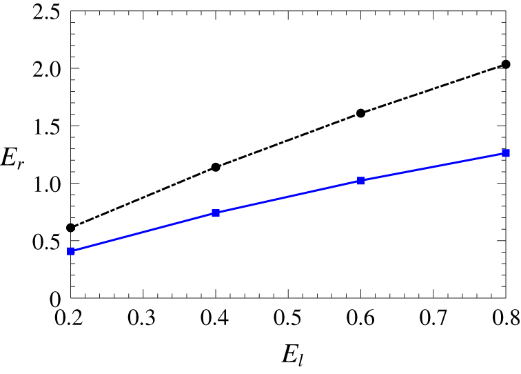
Accordingly, the downstream  $E_{r}$ can be obtained based on the downstream density
 $\unicode[STIX]{x1D70C}_{2}$, which actually represents the densest part of the shock wave. The values of
 $E_{r}$ are shown in figure 1, where the Mach number is equal to 2 and 4, respectively, with
 $E_{l}$ ranging from 0.2 to 0.8. Here, the Mach number is defined as
 $Ma=U_{1}/\sqrt{\unicode[STIX]{x1D6FE}RT_{1}}$, with
 $\unicode[STIX]{x1D6FE}=5/3$ being the specific heat ratio for monatomic gases. We can see from figure 1 that the mean free path of molecules ranges from half to twice the molecular diameter for the considered cases. Note that the reduced density
 $\unicode[STIX]{x1D702}$ is also often used to represent the degree of denseness in dense gases (Frezzotti Reference Frezzotti1998).
The downstream dimensionless parameter  $E_{r}$ for
 $Ma=2$ (solid line) and 4 (dash-dotted line) against the upstream
 $E_{l}$.

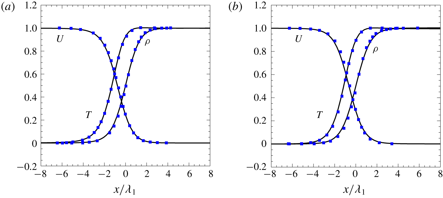
Comparison of the normalized  $\unicode[STIX]{x1D70C}$,
 $U$ and
 $T$, obtained from the Monte Carlo method by Frezzotti & Sgarra (Reference Frezzotti and Sgarra1993) (solid squares) and the FSM (solid line) of solving the Enskog equation at (a)
 $Ma=3$ and
 $E_{l}=0$, and (b)
 $Ma=4$ and
 $E_{l}=0.2$.
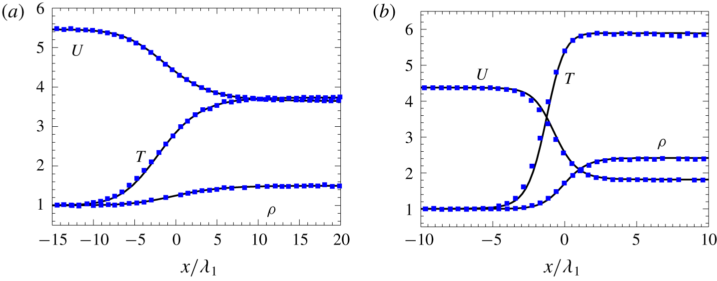
Comparison of  $\unicode[STIX]{x1D70C}$,
 $U$ and
 $T$, obtained from the MD method by Frezzotti (Reference Frezzotti1998) (solid squares) and the FSM of solving the Enskog equation (solid line) at (a)
 $Ma=3$,
 $V_{p}=1.8257$ and
 $E_{l}=2.9831$ (
 $\unicode[STIX]{x1D702}=0.2$), and (b)
 $Ma=4$,
 $V_{p}=2.5674$ and
 $E_{l}=0.4825$ (
 $\unicode[STIX]{x1D702}=0.05$). (Note that the original MD data of the velocity and the
 $x$-axis in Frezzotti (Reference Frezzotti1998) were presented in units of
 $RT_{1}$ and
 $m/\sqrt{2}\unicode[STIX]{x03C0}\unicode[STIX]{x1D70E}^{2}\unicode[STIX]{x1D70C}_{1}$, respectively.)
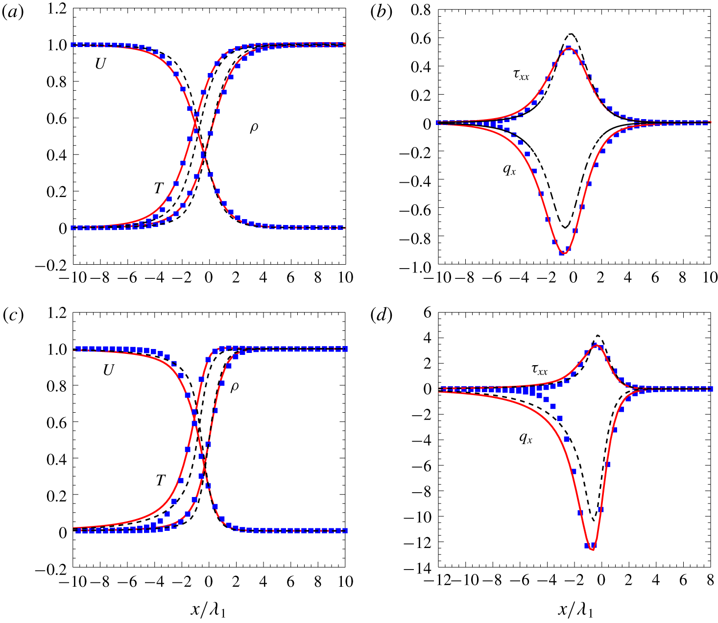
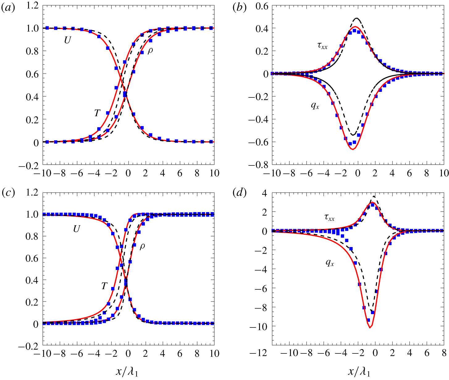
(a,c) The normalized  $\unicode[STIX]{x1D70C}$,
 $U$ and
 $T$; and (b,d) heat flux
 $q_{x}$ and shear stress
 $\unicode[STIX]{x1D70F}_{xx}$. Here
 $E_{l}=0$,
 $Ma=2$ (first row) and
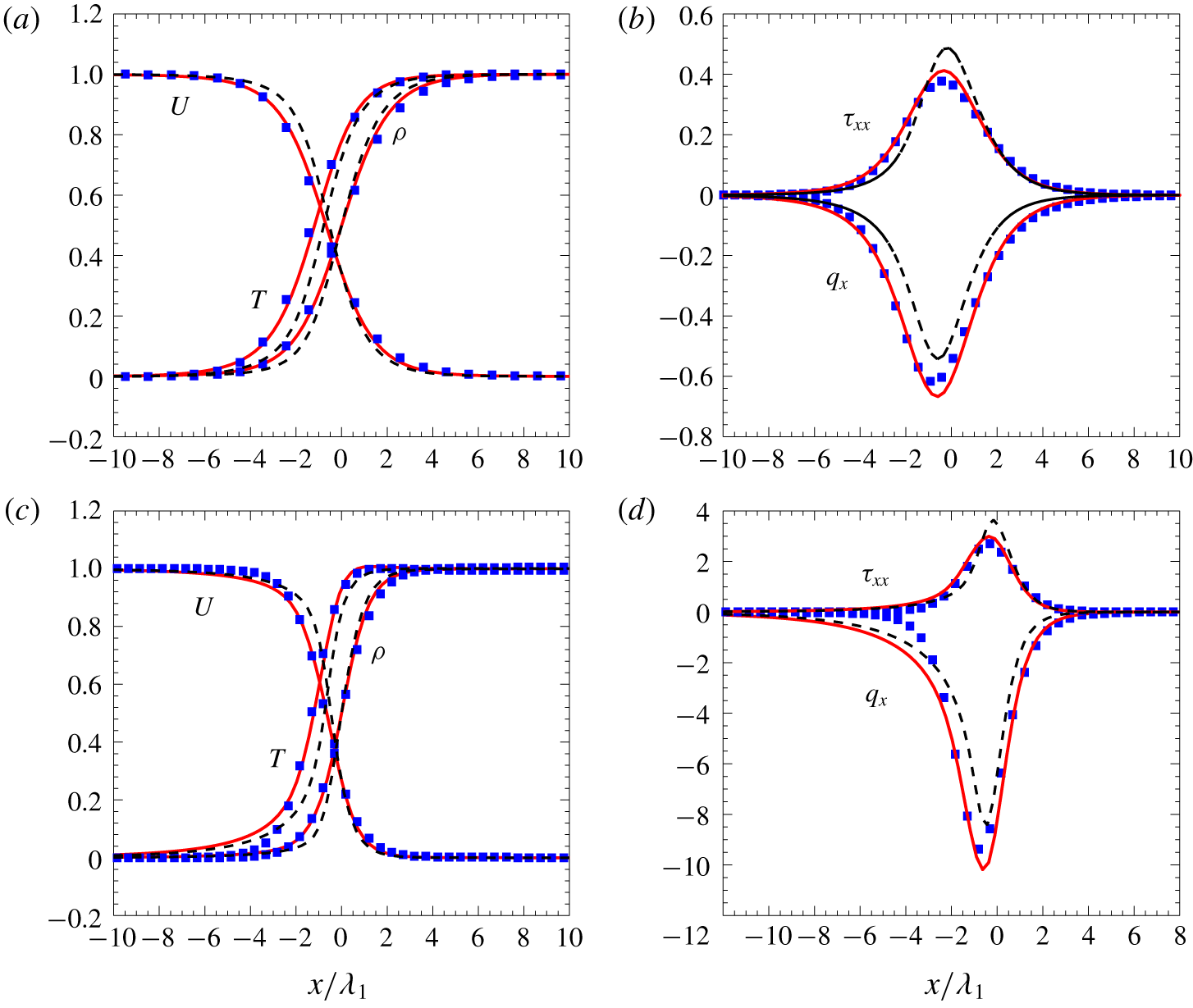
 $Ma=4$ (second row), obtained from the BGK–Enskog model (dashed line), the Shakhov–Enskog model (solid line) and the Enskog equation (solid squares).
In our simulations, the computational domain is set to be  $[-50,50]$ (in units of
 $\unicode[STIX]{x1D706}_{1}$), which is uniformly meshed by 200 points. The molecular velocity space truncated at
 $[-15,15]$ (in units of
 $v_{m}$) is discretized by the mid-point rule with 200 uniform points. The macroscopic quantities
 $W$ are normalized as
 $\bar{W}=(W-W_{1})/(W_{2}-W_{1})$, where the subscripts ‘1’ and ‘2’ denote the quantities upstream and downstream from the shock, respectively; the heat flux and shear stress are presented in units of
 $\unicode[STIX]{x1D70C}_{1}v_{m}^{3}/2$ and
 $\unicode[STIX]{x1D70C}_{1}v_{m}^{2}/2$, respectively. Note that, in what follows, the bar over
 $W$ has been removed for the sake of simplicity, and the
 $x$-axis has been shifted for all the considered quantities so that
 $\unicode[STIX]{x1D70C}(x=0)=(\unicode[STIX]{x1D70C}_{1}+\unicode[STIX]{x1D70C}_{2})/2$.
(a,c) The normalized  $\unicode[STIX]{x1D70C}$,
 $U$ and
 $T$; and (b,d) heat flux
 $q_{x}$ and shear stress
 $\unicode[STIX]{x1D70F}_{xx}$. Here,
 $E_{l}=0.2$,
 $Ma=2$ (first row) and
 $Ma=4$ (second row), obtained from the BGK–Enskog model (dashed line), the Shakhov–Enskog model (solid line) and the Enskog equation (solid squares). Note that the relaxation time given by (2.18) is used in both the BGK–Enskog and the Shakhov–Enskog models.
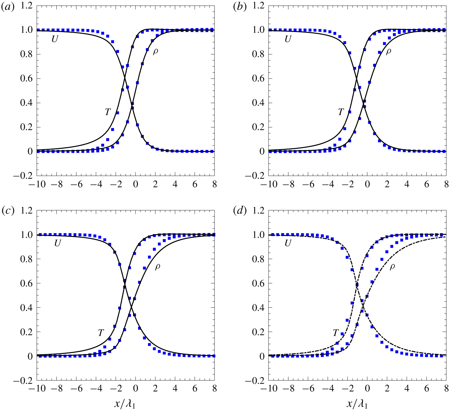
The profiles of normalized  $\unicode[STIX]{x1D70C}$,
 $U$ and
 $T$ at
 $Ma=2$: (a)
 $E_{l}=0.2$, (b)
 $E_{l}=0.4$, (c)
 $E_{l}=0.6$ and (d)
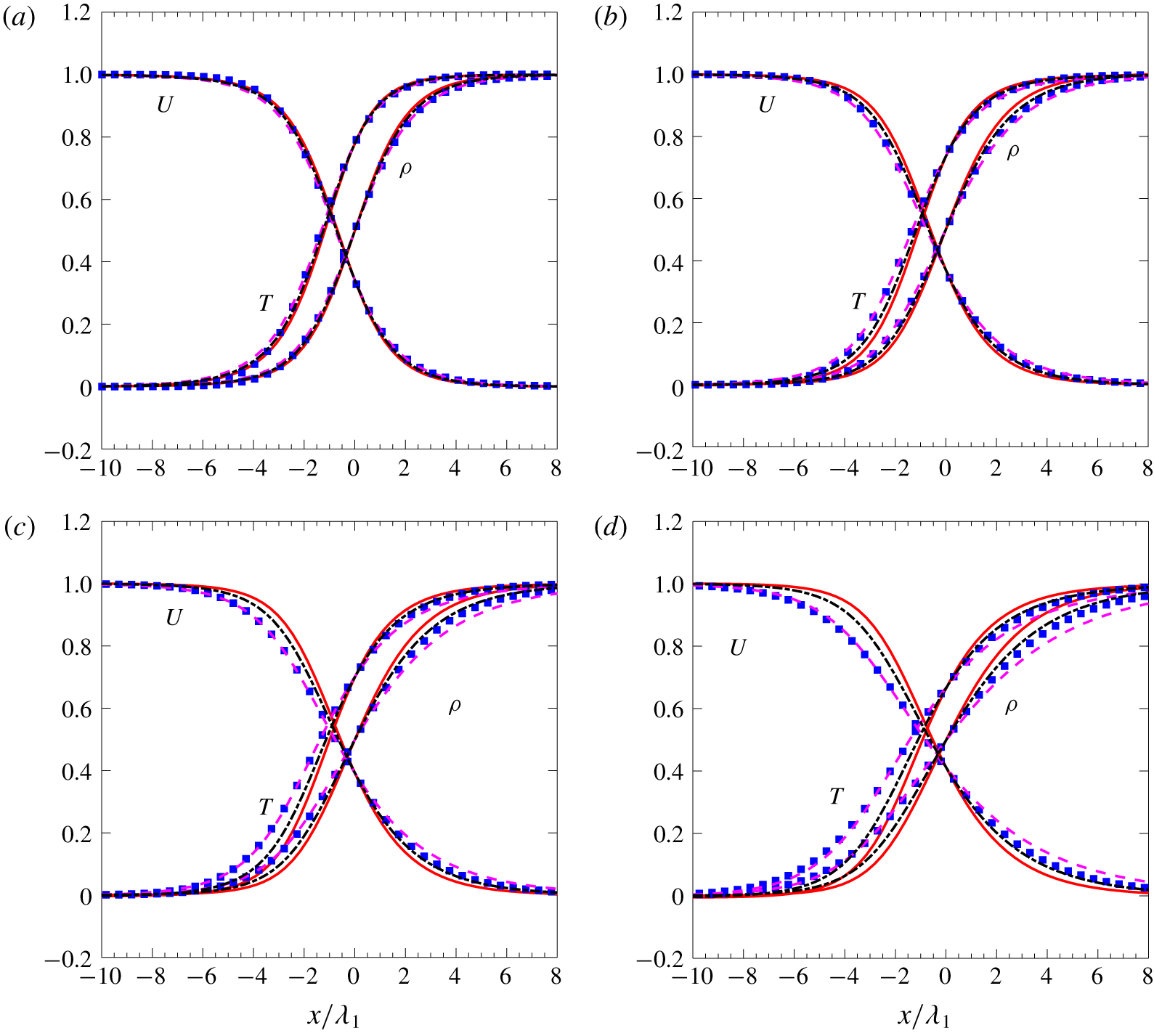
 $E_{l}=0.8$. The solid squares are the results from the Enskog equation, while the dashed, solid and dash-dotted lines are the results of the Shakhov–Enskog model with the relaxation time of (2.17), (2.18) and (2.19), respectively.

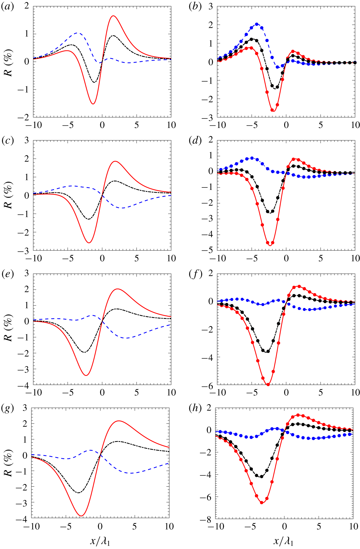
The relative difference  $R(\%)\,(R=100[W_{Shakhov{-}Enskog}/W_{Enskog}-1])$ for the density (left column) and the temperature (right column) at
 $Ma=2$: (a,b)
 $E_{l}=0.2$, (c,d)
 $E_{l}=0.4$, (e,f)
 $E_{l}=0.6$ and (g,h)
 $E_{l}=0.8$. Here
 $W_{Shakhov{-}Enskog}$ and
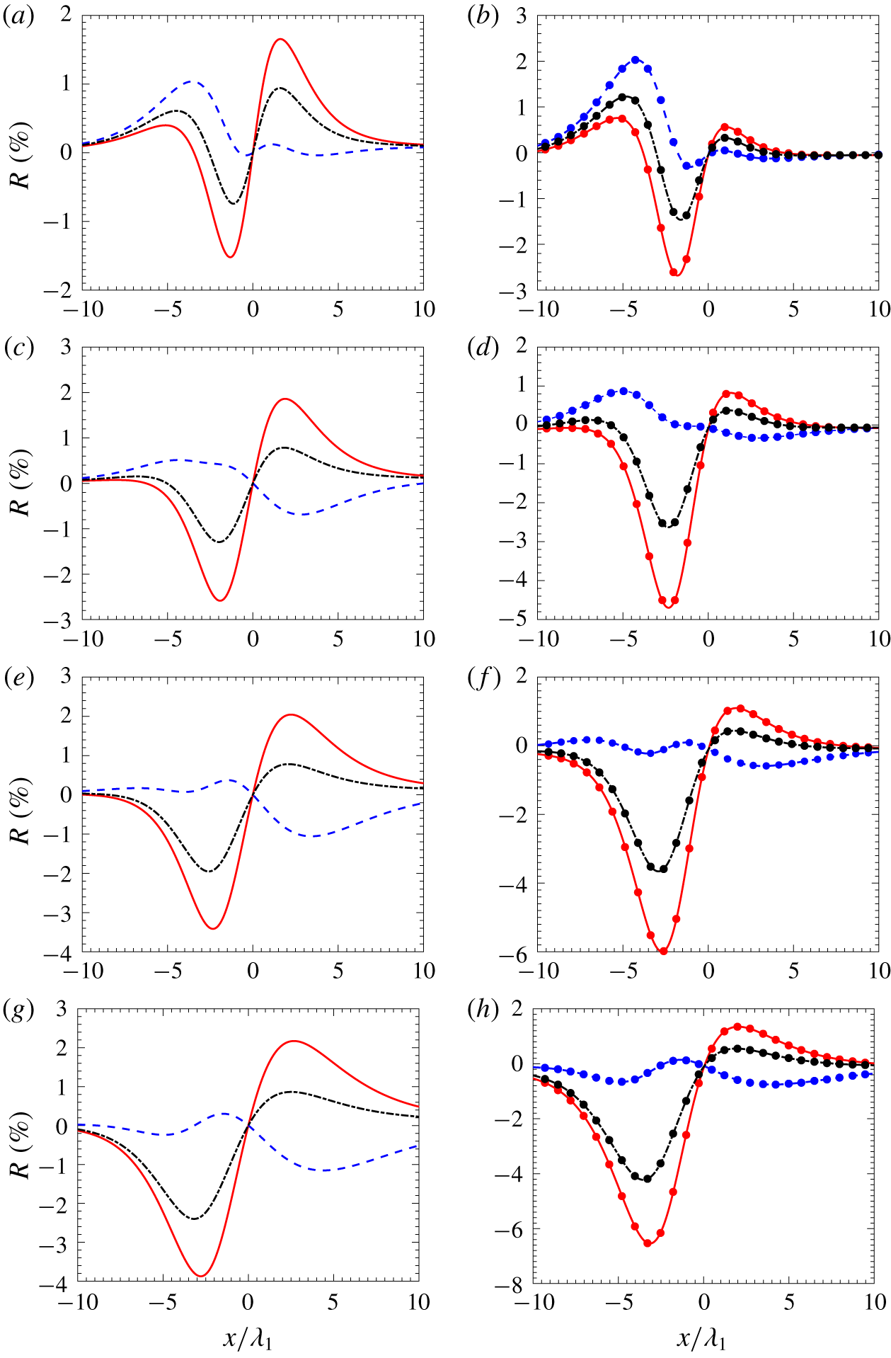
 $W_{Enskog}$ represent the results from the Shakhov–Enskog model and the Enskog equation, respectively. In the left column, the dashed, solid and dash-dotted lines are the relative density difference for the Shakhov–Enskog model using (2.17), (2.18) and (2.19), respectively. Accordingly, in the right column, these lines with the solid circles are the relative temperature difference.
The profiles of normalized  $\unicode[STIX]{x1D70C}$,
 $U$ and
 $T$ at
 $Ma=3$, with (a)
 $E_{l}=0.2$, (b)
 $E_{l}=0.4$, (c)
 $E_{l}=0.6$ and (d)
 $E_{l}=0.8$. The solid squares are the results from the Enskog equation, while the solid lines are the results of the Shakhov–Enskog model with the relaxation time of (2.17).

The profiles of normalized  $\unicode[STIX]{x1D70C}$,
 $U$ and
 $T$ at
 $Ma=4$, with (a)
 $E_{l}=0.2$, (b)
 $E_{l}=0.4$, (c)
 $E_{l}=0.6$ and (d)
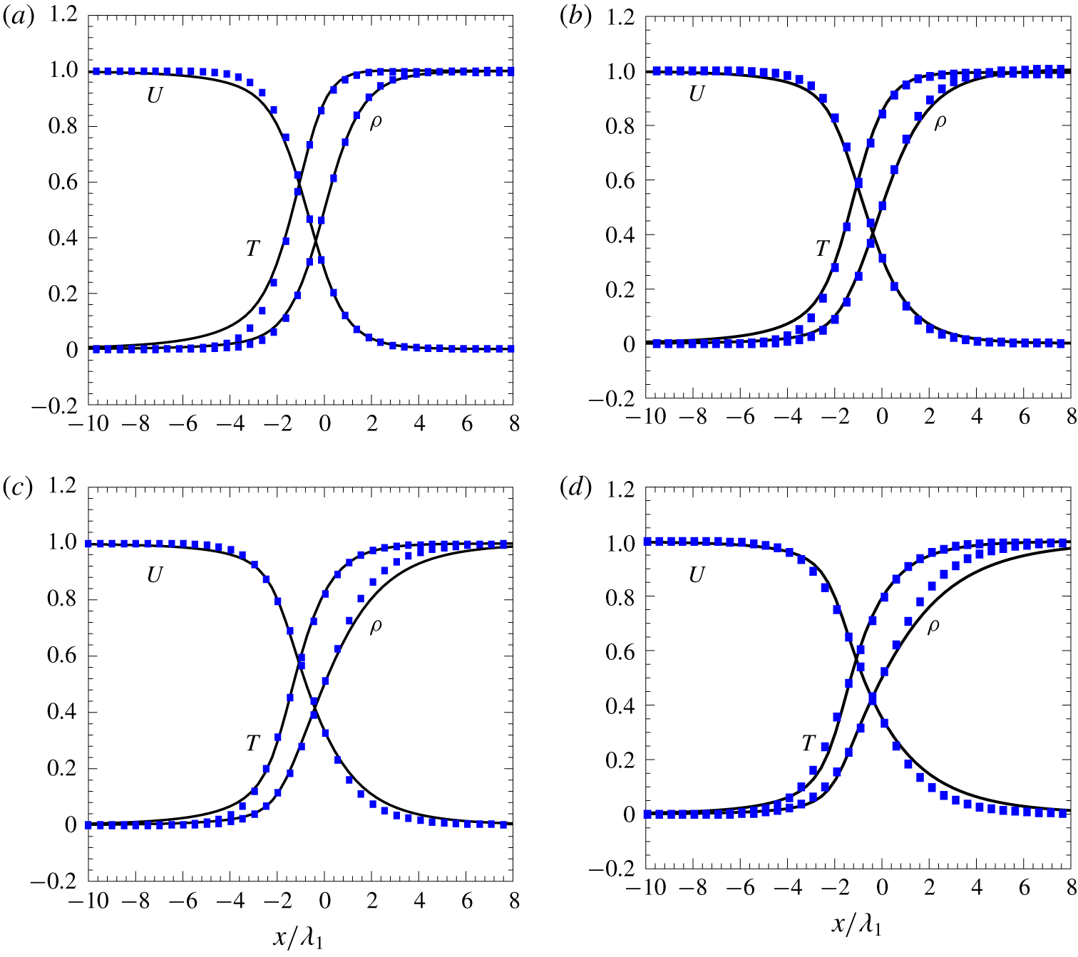
 $E_{l}=0.8$. The solid squares are the results from the Enskog equation, while the solid lines are the results of the Shakhov–Enskog model with the relaxation time of (2.17).

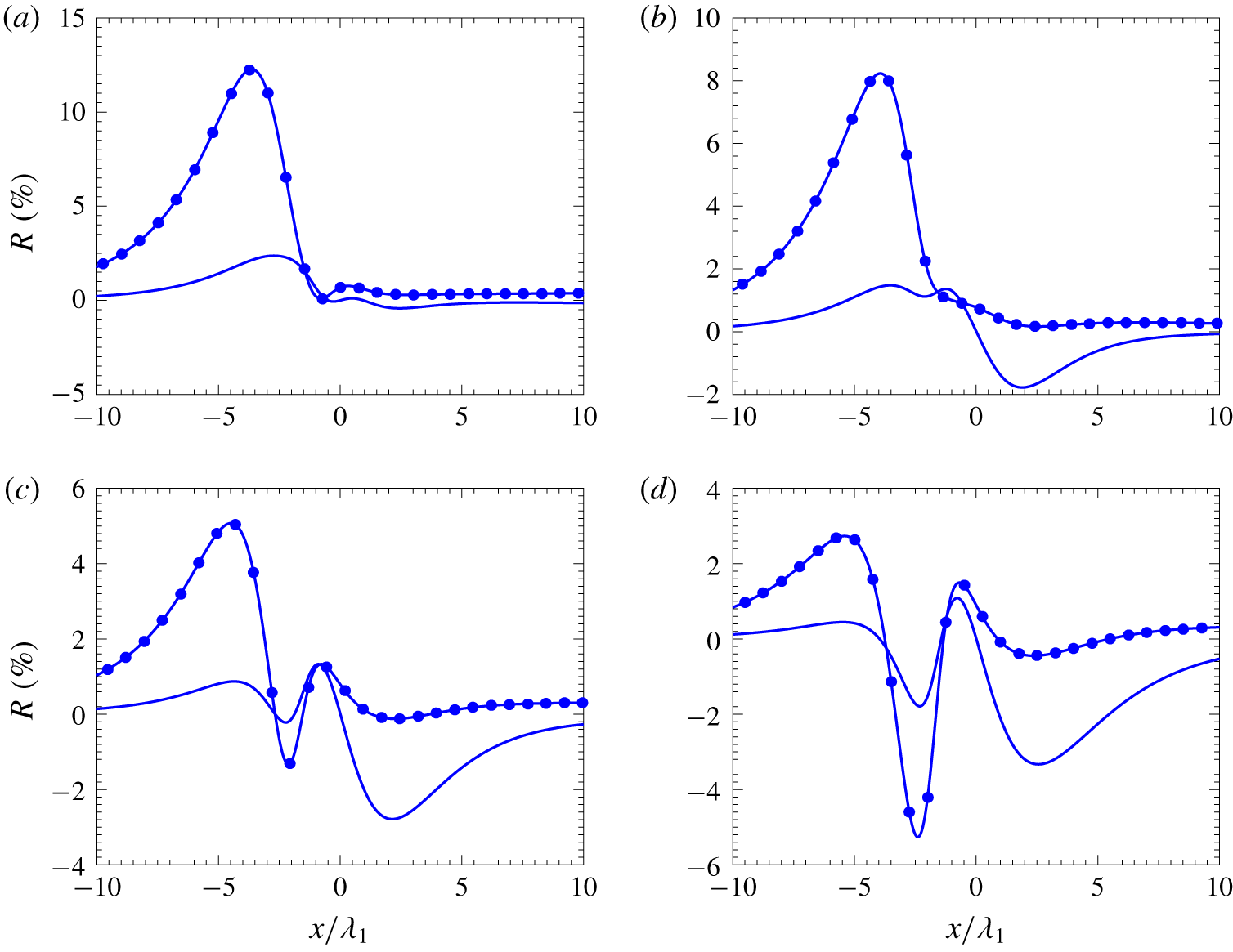
The relative difference in the macroscopic quantities  $R(\%)$ for
 $Ma=3$, obtained from the Shakhov–Enskog model using the relaxation time of (2.17): (a)
 $E_{l}=0.2$, (b)
 $E_{l}=0.4$, (c)
 $E_{l}=0.6$ and (d)
 $E_{l}=0.8$. The relative difference in the density and temperature are represented by the solid line and the solid line with solid circles, respectively.

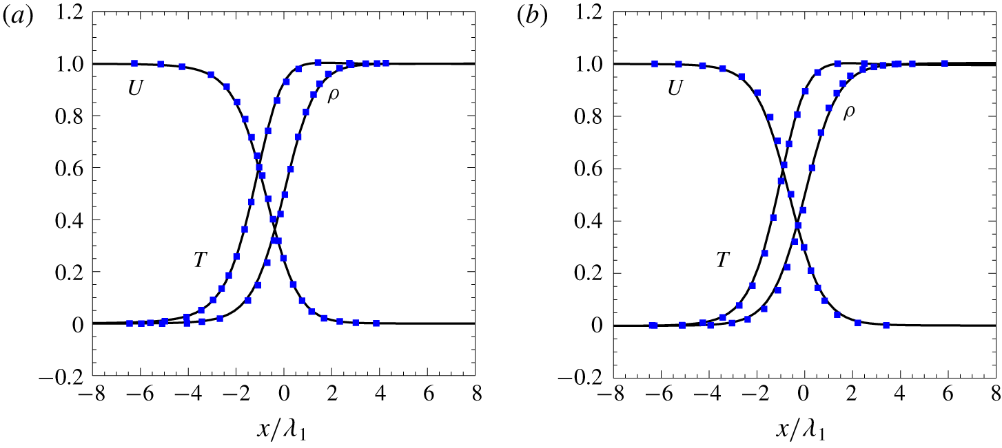
In order to evaluate accuracy of the FSM solving the Enskog equation for a normal shock wave, the normalized density, velocity and temperature computed from the Enskog equation are compared with those of the Monte Carlo method (Frezzotti & Sgarra Reference Frezzotti and Sgarra1993) as shown in figure 2, where the RDF of (2.4) is applied in this case for consistent comparison. Clearly, excellent agreement between these two methods is achieved for  $Ma=4$ in the limits both of a dilute gas
 $(E_{l}=0)$ and of a moderately dense gas of
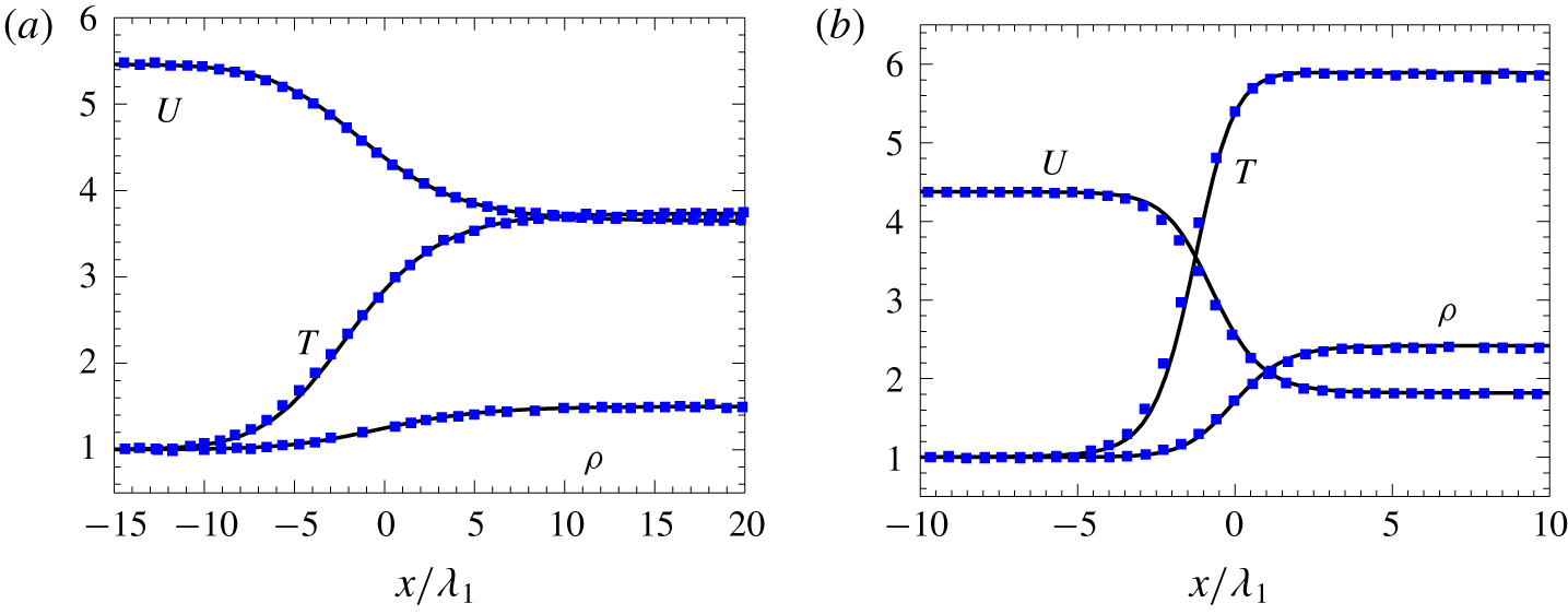
 $E_{l}=0.2$. Figure 3 shows the accuracy of the FSM solving the Enskog equation by comparing the computed macroscopic variables with the MD data (Frezzotti Reference Frezzotti1998). The MD simulation was conducted on a tube with two specularly reflecting endwalls, one of which is at rest, whereas the other one is a piston moving at a constant speed
 $V_{p}$. The piston velocity of
 $V_{p}=1.8257$ and 2.5674 can generate shocks moving at
 $Ma=3$ and 4, respectively, for which the upstreaming
 $E_{l}=2.9831$ (
 $\unicode[STIX]{x1D702}=0.2$) and
 $E_{l}=0.4825$ (
 $\unicode[STIX]{x1D702}=0.05$) are simulated. It is noted from figure 3 that, even for such a high degree of denseness, very good agreement between these two methods can be observed. Therefore, in what follows, solutions of the Enskog equation will serve as the benchmark to validate the proposed Shakhov–Enskog model. Note that (2.3) will be applied in the following simulations, since it strikes a balance between simplicity and accuracy (Frezzotti Reference Frezzotti1997a).
3.2 Comparison of the Shakhov–Enskog model and the BGK–Enskog model
The normalized macroscopic variables  $W$ in the limit case of dilute gases, i.e.
 $E_{l}=0$, for
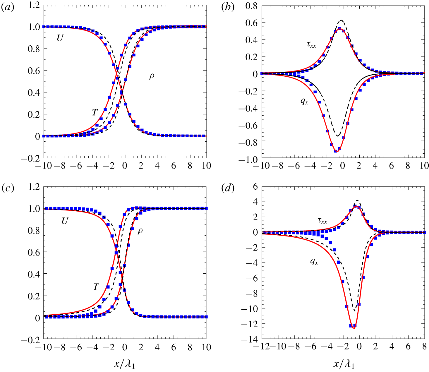
 $Ma=2$ and 4 computed from the Enskog equation, and the BGK–Enskog and Shakhov–Enskog models are shown in figures 4(a) and 4(c); the corresponding heat flux and translational shear stress are presented in figures 4(b) and 4(d). The shear stress due to the translational motion of gas molecules
 $\unicode[STIX]{x1D70F}_{xx}$ can be computed as
 $$\begin{eqnarray}\unicode[STIX]{x1D70F}_{xx}=\int c_{x}^{2}\,f\,\text{d}\unicode[STIX]{x1D743}-p_{0}.\end{eqnarray}$$
When  $E_{l}=0$ and
 $\unicode[STIX]{x1D712}$ is equal to unity, the collision operators of the Enskog equation, and the BGK–Enskog and Shakhov–Enskog models reduce to those of the Boltzmann equation, and the BGK and Shakhov models, respectively. We notice that visible deviations appear mainly upstream, where the degree of non-equilibrium is greater than that downstream due to the lower density before the shock. The BGK model shows a large discrepancy from the Enskog equation not only for the temperature and heat flux, which are directly relevant to the Prandtl number, but also for the density, velocity and shear stress, while the results of the Shakhov–Enskog model agree well with those of the Enskog equation. These findings are consistent with the previous studies of shock wave structure (Li & Zhang Reference Li and Zhang2008; Xu & Huang Reference Xu and Huang2011; Chen, Xu & Cai Reference Chen, Xu and Cai2015; Li et al. Reference Li, Peng, Zhang and Yang2015).
Similar phenomena can also be observed in figure 5 for  $Ma=2$ and 4 with
 $E_{l}=0.2$, except the early rising of temperature and heat flux upstream of the shock. This is due to the well-acknowledged cause that the relaxation time in the model equation, which is independent of the molecular velocity, becomes less accurate for high-Mach-number flows. This is also the reason that the temperature field and heat flux in the case of
 $Ma=4$ exhibit larger discrepancy than those of
 $Ma=2$, when compared with the corresponding results of the Enskog equation; see figures 4 and 5. For example, the maximum relative difference in the temperature for
 $Ma=2$ and 4 is approximately
 $3\,\%$ and
 $30\,\%$, respectively.
3.3 Evaluation of the Shakhov–Enskog model
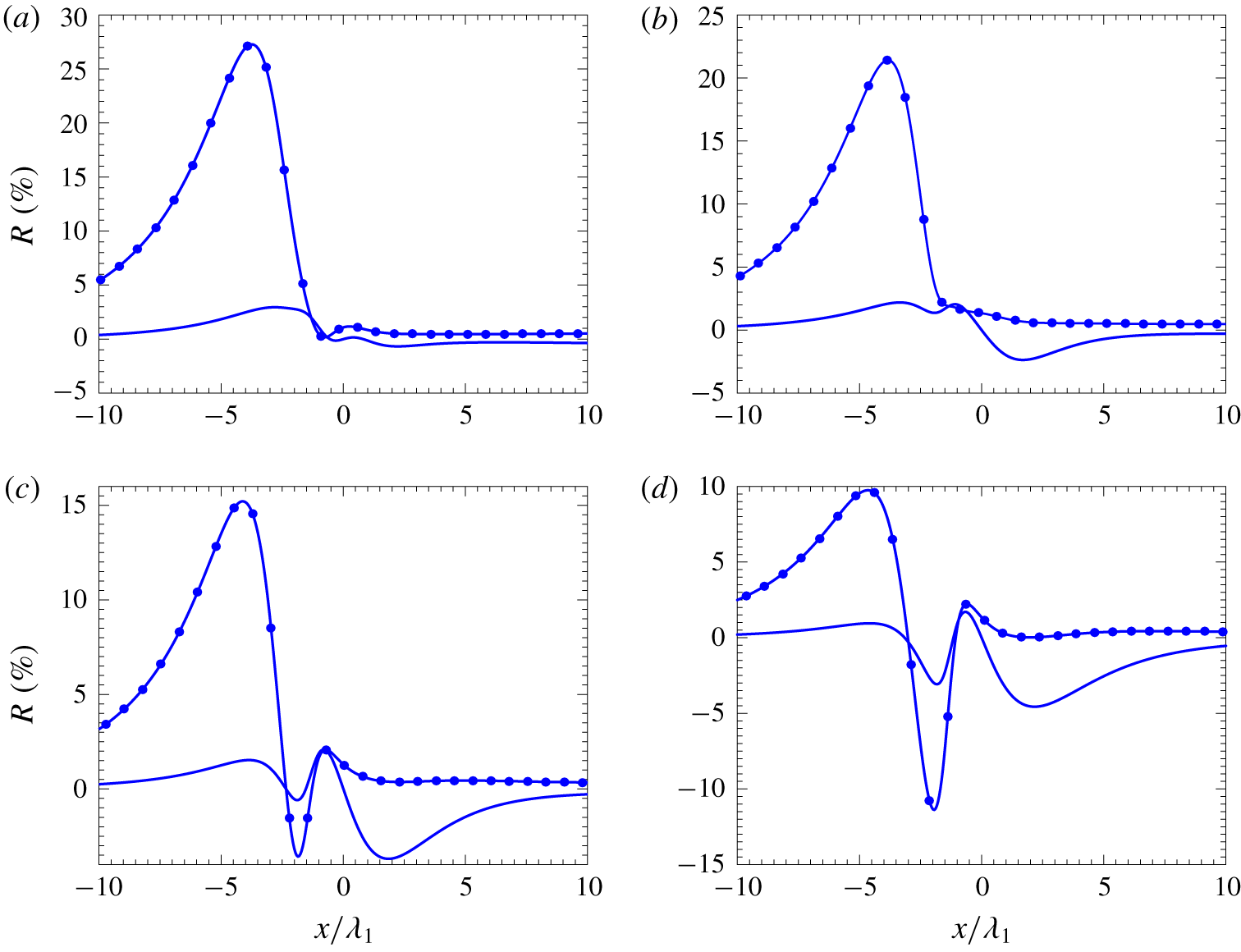
The relative difference in the macroscopic quantities  $R(\%)$ for
 $Ma=4$ obtained from the Shakhov–Enskog model using the relaxation time of (2.17): (a)
 $E_{l}=0.2$, (b)
 $E_{l}=0.4$, (c)
 $E_{l}=0.6$ and (d)
 $E_{l}=0.8$. The relative differences in the density and temperature are represented by the solid line and the solid line with solid circles, respectively.

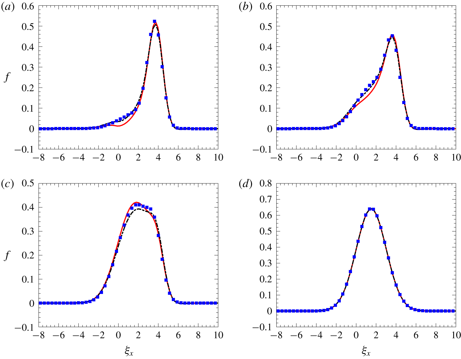
The marginal reduced velocity distribution function  $f$ as a function of the molecular velocity
 $\unicode[STIX]{x1D709}_{x}$ at
 $x/\unicode[STIX]{x1D706}_{1}=-1.5$ (a),
 $-0.5$ (b), 0.5 (c) and 10 (d). The solid squares are the results from the Enskog equation, while the dash-dotted and solid lines are the results of the Shakhov–Enskog model with the relaxation time of (2.17) and (2.18), respectively. The molecular velocity
 $\unicode[STIX]{x1D709}_{x}$ is in units of the most probable velocity
 $v_{m}$.

We now evaluate the Shakhov–Enskog model with different relaxation time  $\tilde{\unicode[STIX]{x1D70F}}$ by comparing with the Enskog equation. The normalized macroscopic variables for
 $Ma=2$ with
 $E_{l}$ from 0.2 to 0.8 are shown in figure 6(a–d). It can be seen that, when
 $E_{l}=0.2$, the results of the Shakhov–Enskog model with the relaxation time given by (2.17), (2.18) and (2.19), respectively, are in good agreement with the Enskog solutions. With the increase of
 $E_{l}$, the deviation of the Shakhov–Enskog model from the Enskog equation becomes more pronounced. We notice that, for the case
 $E_{l}=0.4$, the profiles calculated from the proposed model with the relaxation time of (2.18) show a more visible difference from those of the Enskog equation, while the results computed from the model with (2.17) and (2.19) still show a good agreement with the reference solutions. However, when
 $E_{l}\geqslant 0.6$, both (2.18) and (2.19) cannot reproduce acceptable shock structure profiles, particularly upstream, where the Shakhov–Enskog model clearly underestimates the macroscopic variables. When using (2.17), as expected, the kinetic model overall shows a better agreement with the Enskog equation for all values of
 $E_{l}$; in particular, the early rise of temperature upstream seems to be accurately captured by the Shakhov–Enskog model.
The performance of the Shakhov–Enskog model with different formulae for the relaxation time can be quantitatively explained by the relative difference in density and temperature, which is shown in the left and right columns of figure 7, respectively. Note that the relative difference in velocity has the same magnitude as that in density but with an opposite sign, which is not presented. It is clearly found that, in most of the region of the shock structure, the maximum relative difference in the macroscopic variables computed from the present model with (2.17) is less than  $2\,\%$, which is the smallest amongst these three formulae. When using the relaxation time of (2.18), the obtained temperature could differ from the Enskog solution by
 $6\,\%$ at
 $E_{l}=0.6$; meanwhile, the model with (2.19) can also overestimate the temperature by
 $4\,\%$ at
 $E_{l}=0.8$. The above results show that the proposed Shakhov–Enskog model with the relaxation time of (2.17), which adopts the viscosity coefficient accounting for both kinetic and potential contributions, as expected provides the best prediction of the shock structure. Therefore, unless otherwise stated, the relaxation time of (2.17) will be applied in the Shakhov–Enskog model in the following simulations.
The results obtained from the Shakhov–Enskog model with (2.17) and the Enskog equation are further presented in figures 8 and 9 for  $Ma=3$ and
 $Ma=4$, respectively. With the increase of
 $E_{l}$, despite the growing underestimate of the density near the shock front (
 $x/\unicode[STIX]{x1D706}_{1}>2$), overall good agreement between the two sets of results is observed. The same as the case of
 $Ma=2$, for such high-Mach-number flows, the conspicuous overestimate of the temperature by the present model arises before the shock front as well; this is due to the inherent drawback of the Shakhov model. Meanwhile, it is interesting to see that the overestimate of the temperature becomes less significant when the Mach number increases, which may be attributed to the reducing non-equilibrium effect due to the increase of
 $E_{l}$ at the upstream of the shock.
The discrepancy between the proposed model and the Enskog equation is further examined by the relative differences in the shock profiles, which are shown in figures 10 and 11 for the cases of  $Ma=3$ and 4, respectively. Note that the relative difference in the velocity is not presented here. We can see that the Shakhov–Enskog model can reproduce the density and velocity profiles accurately, with the overall relative difference being smaller than
 $4\,\%$ and
 $10\,\%$ for
 $Ma=3$ and 4, respectively, whereas there are large deviations in the temperature profile from the Enskog solution with a maximum relative difference up to
 $15\,\%$ and
 $30\,\%$, respectively, at
 $E_{l}=0.2$. Meanwhile, as clearly shown, the maximum difference of temperature is smaller at larger
 $E_{l}$. This deficiency of the proposed model is inherited from the Shakhov collision operator itself, instead of the Enskog equation. However, the relative difference in the density and velocity profiles is less than
 $5\,\%$, as shown in figures 7, 10 and 11, suggesting that the Shakhov–Enskog model can capture rarefaction effects reasonably well in dense gases. For very dense gases, where the molecules are nearly in constant contact, both the Enskog equation and its model become inaccurate, which is reflected in the results for large
 $E_{l}$.
The differential performance of the Shakhov–Enskog model when using different types of relaxation time can be essentially explained from the microscopic VDF. The parallel VDFs as a function of  $\unicode[STIX]{x1D709}_{x}$ at different locations of the shock are shown in figure 12, where the Shakhov–Enskog model with the relaxation time of (2.17) and (2.18) for
 $Ma=4$ and
 $E_{l}=0.4$ are examined as an example. The results are similar for the other parameters. It is noticed that the VDFs computed from the Shakhov–Enskog model with (2.17) are better than the model with (2.18), when compared with the Enskog equation, particularly in the region
 $\unicode[STIX]{x1D709}_{x}\in (-v_{m},2v_{m})$; see figure 12(a,b). In addition, as we see from figure 12(d), at
 $x/\unicode[STIX]{x1D706}_{1}=10$, where it is far from the shock centre, the proposed model can accurately reproduce VDF close to equilibrium. Note that one of the potential drawbacks inherited from the Shakhov collision operator, i.e. the negative value of VDF, does not appear in the above simulations.
4 Concluding remarks
In this work, a kinetic model has been proposed to simplify the Enskog equation for non-equilibrium flow of dense gases using the kinetic Shakhov model, which can recover the correct Prandtl number of monatomic dilute gases. The propagation of a normal shock wave in a dense gas is simulated to validate the proposed Shakhov–Enskog model against the FSM solution of the Enskog equation. In comparison with the BGK–Enskog model, the Shakhov–Enskog model with a correct Prandtl number agrees better with the Enskog equation, not only for the temperature and heat flux, which are directly relevant to the Prandtl number, but also for the density, velocity and shear stress.
The relaxation time of (2.17) accounts for both the kinetic and collisional contributions to the momentum and energy transfer, so the Shakhov–Enskog model can predict the shock profiles well. Surprisingly, with the use of (2.17), the early rising of temperature as observed in the dilute gases is also much improved.
In conclusion, the proposed Shakhov–Enskog model is capable of describing the momentum and energy transfer inside a shock, when the maximum local mean free path of the gas molecules is greater than the size of the gas molecules. More importantly, for all the simulations in this study, the computational cost for the DVM solution of the Shakhov–Enskog model is at least two orders less than the FSM solution of the Enskog equation. The current work does not consider the gas–surface interactions, which are an important but difficult research challenge for the surface-bounded non-equilibrium flow of dense gases. When the attractive force between molecules is properly considered, the Shakhov–Enskog model may also provide a new way of modelling the non-equilibrium behaviour of multiphase flows.
Acknowledgements
Financial support from the UK Engineering and Physical Sciences Research Council (EPSRC) under grants EP/M021475/1, EP/R041938/1 and EP/R029598/1 is gratefully acknowledged. This work is also supported by the College of Petroleum Engineering and Geosciences, King Fahd University of Petroleum and Minerals, Saudi Arabia.
Declaration of interests
The authors declare no competing interests.
Appendix A. Reduction of the Shakhov–Enskog model for one-dimensional case
Since only a one-dimensional shock wave is considered in this study, two reduced velocity distribution functions are introduced to cast the three-dimensional molecular velocity space  $(\unicode[STIX]{x1D709}_{x},\unicode[STIX]{x1D709}_{y},\unicode[STIX]{x1D709}_{z})$ into one dimension as
 $$\begin{eqnarray}\displaystyle & \displaystyle g=\int f(\boldsymbol{x},\unicode[STIX]{x1D743},t)\,\text{d}\unicode[STIX]{x1D709}_{y}\,\text{d}\unicode[STIX]{x1D709}_{z}, & \displaystyle\end{eqnarray}$$
 $$\begin{eqnarray}\displaystyle & \displaystyle h=\int (\unicode[STIX]{x1D709}_{y}^{2}+\unicode[STIX]{x1D709}_{z}^{2})f(\boldsymbol{x},\unicode[STIX]{x1D743},t)\,\text{d}\unicode[STIX]{x1D709}_{y}\,\text{d}\unicode[STIX]{x1D709}_{z}. & \displaystyle\end{eqnarray}$$
 $g$ and
 $h$ are obtained, the macroscopic variables can be computed as
 $$\begin{eqnarray}\unicode[STIX]{x1D70C}=\int g\,\text{d}\unicode[STIX]{x1D709}_{x},\quad \unicode[STIX]{x1D70C}U=\int \unicode[STIX]{x1D709}_{x}g\,\text{d}\unicode[STIX]{x1D709}_{x},\quad T=\frac{1}{3\unicode[STIX]{x1D70C}R}\int (c_{x}^{2}g+h)\,\text{d}\unicode[STIX]{x1D709}_{x},\end{eqnarray}$$
and the high-order moments of interest, i.e. the shear stress  $\unicode[STIX]{x1D70F}_{xx}$ and heat flux
 $q_{x}$, are given by
 $$\begin{eqnarray}\unicode[STIX]{x1D70F}_{xx}=\int c_{x}^{2}g-\unicode[STIX]{x1D70C}RT,\quad q_{x}=\frac{1}{2}\int c_{x}(c_{x}^{2}g+h)\,\text{d}\unicode[STIX]{x1D709}_{x}.\end{eqnarray}$$
The governing equations for the two reduced VDFs can be deduced from (2.13) as
 $$\begin{eqnarray}\displaystyle & \displaystyle \frac{\unicode[STIX]{x2202}g}{\unicode[STIX]{x2202}t}+\unicode[STIX]{x1D709}_{x}\frac{\unicode[STIX]{x2202}g}{\unicode[STIX]{x2202}x}=-\frac{1}{\tilde{\unicode[STIX]{x1D70F}}}[g-g^{S}]+J_{a,g}^{1}+J_{b,g}^{1}, & \displaystyle\end{eqnarray}$$
 $$\begin{eqnarray}\displaystyle & \displaystyle \frac{\unicode[STIX]{x2202}h}{\unicode[STIX]{x2202}t}+\unicode[STIX]{x1D709}_{x}\frac{\unicode[STIX]{x2202}h}{\unicode[STIX]{x2202}x}=-\frac{1}{\tilde{\unicode[STIX]{x1D70F}}}[h-h^{S}]+J_{a,h}^{1}+J_{b,h}^{1}, & \displaystyle\end{eqnarray}$$
 $g^{S}=g^{eq}+g_{Pr}$ and
 $h^{S}=h^{eq}+h_{Pr}$, with
 $$\begin{eqnarray}\displaystyle & \displaystyle g^{eq}=\frac{\unicode[STIX]{x1D70C}}{(2\unicode[STIX]{x03C0}RT)^{1/2}}\exp \left[-\frac{c_{x}^{2}}{2RT}\right], & \displaystyle\end{eqnarray}$$
 $$\begin{eqnarray}\displaystyle & \displaystyle h^{eq}=2RTg^{eq}, & \displaystyle\end{eqnarray}$$
 $$\begin{eqnarray}\displaystyle & \displaystyle g_{Pr}=(1-\Pr )\frac{c_{x}q_{x}}{5p_{0}RT}\left[\frac{c_{x}^{2}}{RT}-3\right]g^{eq}, & \displaystyle\end{eqnarray}$$
 $$\begin{eqnarray}\displaystyle & \displaystyle h_{Pr}=(1-\Pr )\frac{c_{x}q_{x}}{5p_{0}RT}\left[\frac{c_{x}^{2}}{RT}-1\right]h^{eq}, & \displaystyle\end{eqnarray}$$
 $$\begin{eqnarray}\displaystyle & \displaystyle J_{a,g}^{1}=-g^{eq}b\unicode[STIX]{x1D70C}c_{x}\unicode[STIX]{x2202}_{x}\unicode[STIX]{x1D712}, & \displaystyle\end{eqnarray}$$
 $$\begin{eqnarray}\displaystyle & \displaystyle J_{b,g}^{1}=-g^{eq}b\unicode[STIX]{x1D70C}\unicode[STIX]{x1D712}\left\{2c_{x}\unicode[STIX]{x2202}_{x}\ln \unicode[STIX]{x1D70C}+\frac{3}{5}\left[\frac{c_{x}^{2}}{RT}-1\right]\unicode[STIX]{x2202}_{x}u_{x}+\frac{3}{10}\left[\frac{c_{x}^{3}}{RT}+\frac{1}{3}c_{x}\right]\unicode[STIX]{x2202}_{x}\ln T\right\},\qquad & \displaystyle\end{eqnarray}$$
 $$\begin{eqnarray}\displaystyle & \displaystyle J_{a,h}^{1}=-h^{eq}b\unicode[STIX]{x1D70C}c_{x}\unicode[STIX]{x2202}_{x}\unicode[STIX]{x1D712}, & \displaystyle\end{eqnarray}$$
 $$\begin{eqnarray}\displaystyle & \displaystyle J_{b,h}^{1}=-h^{eq}b\unicode[STIX]{x1D70C}\unicode[STIX]{x1D712}\left\{2c_{x}\unicode[STIX]{x2202}_{x}\ln \unicode[STIX]{x1D70C}+\frac{3}{5}\left[\frac{c_{x}^{2}}{RT}-\frac{1}{3}\right]\unicode[STIX]{x2202}_{x}u_{x}+\frac{3}{10}\left[\frac{c_{x}^{3}}{RT}+\frac{7}{3}c_{x}\right]\unicode[STIX]{x2202}_{x}\ln T\right\},\qquad & \displaystyle\end{eqnarray}$$
 $\unicode[STIX]{x2202}_{x}$ denotes the derivative with respect to the
 $x$-axis. It is clear that the governing equation for
 $g$ and
 $h$ in (A 4) can be expressed in the following compact form:
 $$\begin{eqnarray}\frac{\unicode[STIX]{x2202}\unicode[STIX]{x1D719}}{\unicode[STIX]{x2202}t}+\unicode[STIX]{x1D709}_{x}\frac{\unicode[STIX]{x2202}\unicode[STIX]{x1D719}}{\unicode[STIX]{x2202}x}=-\frac{1}{\tilde{\unicode[STIX]{x1D70F}}}[\unicode[STIX]{x1D719}-\unicode[STIX]{x1D719}^{S}]+\unicode[STIX]{x1D6FA}_{E,\unicode[STIX]{x1D719}},\end{eqnarray}$$
where the symbol  $\unicode[STIX]{x1D719}$ is used to represent
 $g$ or
 $h$, and
 $\unicode[STIX]{x1D6FA}_{E,\unicode[STIX]{x1D719}}=J_{a,\unicode[STIX]{x1D719}}^{1}+J_{b,\unicode[STIX]{x1D719}}^{1}$. Finally, (A 7) is readily solved by the iterative implicit DVM described by (3.2).