The Jobs Model Forecast for 2008

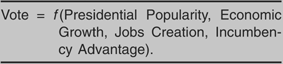
Theoretically, the model views the election as a referendum on the economic and political performance of the president's party, with that party itself having a built-in incumbency advantage. A unique feature of the model is that, as part of economic performance, it includes the actual number of new jobs created in the labor market. Given the nation's increasing income inequality, this distributional variable seems especially important. The overall model expresses itself verbally in Equation 1.

Table 1.

Equation 1: The Jobs Model

This equation, when measured and estimated with ordinary least squares (OLS) regression, over presidential elections, 1952–2004, is shown as Equation 2. Note that, because it is a forecasting equation, all independent variable measures are available well before the election itself.

Table 2.

Equation 2: The Jobs Model

Notes: V = presidential party share of the two-party vote. P = presidential popularity, as measured by the first Gallup Poll in July of the election year. G = gross national product, as percentage change (non-annualized) in GNP (constant dollars) from the fourth quarter of the year prior to the election to the second quarter of the election year, data from the Survey of Current Business. E = elected president running (scored 1) or not (scored 0.5). J = jobs growth, in percentage change in jobs over the first 3.5 years of the president's term; the entries are calculated as follows: (number employed in June of the election year − number employed in January of the inauguration year)/number employed in January of the inauguration year) × 100. The employment numbers are from the Civilian Labor Force (16 years and older), reported in the Bureau of Labor Statistics' Current Population Survey of Households (not seasonally adjusted). I = incumbent party advantage, scored 1 if the incumbent party candidate is the elected president (1956, 1972, 1980, 1984, 1992, 1996, 2004) or following a president who died in office (1948,1964), scored 0 if the incumbent party candidate has a tolerable relationship with the previous president (1952, 1976, 1988), scored −1 if the incumbent party candidate and the president are not united (1960, 1968, 2000): * = statistical significance at 0.05 onetail; the figures in parentheses are t-ratios: R-squared = the coefficient of multiple determination; the adjusted R-squared = the R-squared adjusted for degrees of freedom; SEE = the standard error of estimate; D-W = the Durbin-Watson statistic; N = the 14 presidential election observations, 1952–2004; e = error.

What does the Jobs Model forecast for 2008? We can answer that question by plugging in the relevant independent variable values, shown here as Equation 3: Bush popularity (P) = 31% (July 10–13); GNP change = 0.81%, E = 0.5, so (G × E) = 0.41%; J = 5.75%; I = 0 (George W. Bush and John McCain appear supportive of each other).Footnote ¹

Table 3.

Equation 3: The Jobs Model Forecast for 2008

This forecast means 56.57% of the two-party popular vote will go for Democratic Party candidate Barack Obama. If it comes to pass, it would render the incumbent party the biggest defeat ever experienced across the time period, exceeding even the Democratic loss to Dwight Eisenhower in 1952. The key force behind such a defeat, according to the model, is the extreme unpopularity of President Bush himself. With a mid-summer approval rating of 31%, he stands historically near the bottom of the approval ladder. We know that unpopular presidents can cause their party great suffering at the ballot box, and this is a stellar case in point. In addition to being blamed for Bush's shortcomings in office, the sagging economy helps Senator McCain not at all.Footnote ²

Ballot Box Racism? Estimating the ‘Cost’ of a Black Candidate

In his classic work on data analysis, Tufte (Reference Tufte1974, 63) vividly reminds us of the dangers of “spellbinding extrapolation.” This problem, extrapolating model forecasts well beyond the range of the model data, clearly presents itself here. In the post-World War II time series studied by presidential election forecasters, there have been no major-party candidates who are from a racial minority. Values on this important independent variable—race—have been set at a constant value—White. What happens when the value of this variable changes to Black? Here we try to arrive at some estimate of the effects of such a change in order to adjust, if necessary, our above forecast. This is not an easy task. We explore different scenarios, before arriving at some tentative conclusions.

One possibility is that no racial bias will factor into vote choice, in which case our model estimate would remain unchanged. A first test comes from examination of whether there was a “Bradley effect” in the polls and 2008 Democratic primary vote. In particular, perhaps the pre-election opinion poll estimate for Obama was above his actual vote share. Such a finding might arise from respondents succumbing to the “social desirability” of expressing favorable attitudes about Blacks. Thus, the pressure to yield up a socially desirable answer tends to push some to falsely declare support for Obama. Of course, this so-called Bradley effect may not have occurred in the 2008 primary polls, with respondents simply giving their “true” opinions, accompanied by the usual amount of error.

Suppose variable X is poll support for Obama before the primary, and Y is vote support for Obama in the primary. Then the main hypothesis concerns the difference of means,

where X = the average of the last pre-primary polls reported on the Real Clear Politics web site, by state. Typically, there were three or four such polls in each of these states, N = 30 (including the caucus states of Iowa and Nevada). Y = the percentage vote share in the Democratic nomination contest in that state.

Looking at the results, we observe that the Obama poll average = 41.2%, and the Obama vote average = 47.1%, for a difference of +5.8%. This difference is not statistically significant at 0.05 (and is even is the opposite direction hypothesized). These results continue to hold when the two caucus states are dropped, leaving a non-significant difference of +5.6%. While this is evidence against a Bradley effect, it implies that Obama was getting more support at the ballot box than at the polls. However, the polls also reported preferences for other candidates and for undecided voters, while the vote numbers do not include undecided voters.

Therefore, we calculated for Obama his percentage share of the two-leading candidates total, i.e., the Obama + Hillary Clinton total. In each state, Obama poll percentage share = Obama poll number/(Obama poll number + Clinton poll number). The Obama two-candidate average poll share = 48.8% (where N = 25, excluding states before Super Tuesday since John Edwards was still competing). The Obama vote average for these states = 48.2%, yielding a tiny difference of −0.55%, not statistically significant at 0.05. In these results, any traces of a racial effect from poll to primary are removed. Among Democratic primary voters there simply does not appear to be a race effect, for or against, influencing their stated preferences in the polls.

But, to say that respondents express their true preferences when faced with the choice of a Black candidate is not to say that they favor that candidate. Indeed, it may mean that respondents who do not like a Black candidate, strictly on racial grounds, simply feel free to declare that they will vote for White candidate X. In this way their racism is “hidden,” for they are merely recorded as favoring White candidate X. Assessing the level of this “hidden racism” is extremely difficult. Fortunately, Heerwig and McCabe (Reference Heerwig and McCabe2007) recently made an insightful attempt at such an assessment. They wish to get around possible social desirability bias, where respondents tend to answer favorably when queried directly: “Would you support a Black candidate for president?” For example, in the General Social Survey, as early as 1996, fully 92% of the respondents answered such a question affirmatively. Rather than simply posing this item and tallying the responses, Heerwig and McCabe (Reference Heerwig and McCabe2007) conduct a list experiment. In the control group, subjects were asked about their support for three political statements, while in the treatment group subjects were asked about these same three political statements, plus one more asking about willingness to support a generic Black presidential candidate. (The subjects were asked to report how many of the items on the list they support, but not which specific ones they support.)

Assuming random assignment, a comparison of the treatment and control group means estimates the “true” percentage of those willing to support a Black presidential candidate. The study, done in June 2007 on a representative national American sample, finds that “true support” to be 70%. That percentage is for the total sample. When it is restricted to voters, which are our focus, the figure rises to 77%. However, there is some reason to believe that this estimate is biased downward, because it averages in Democrats who are against Obama merely because on policy grounds they are for, say, Clinton or Edwards. Specifically, among Democrats in the total sample, only 60% say they would be able to vote for a Black presidential candidate, in contrast to 87% for Republicans. The low number for Democrats appears partly a function of their having in mind a concrete Black candidate—Obama—rather than an abstract generic Black candidate. (The survey was done in summer 2007, the period when Obama declared his candidacy.) In that context, the high number for Republicans (of 0.87) may be more accurate for the whole, since Republicans at the time of the survey likely had no serious Black candidate in mind (since no Black Republican had declared).

An observational, as opposed to an experimental, approach compares the “normal vote” for a White Democratic primary candidate to Obama's primary vote. We examine two similar Democratic primary races, matched on relevant characteristics, differing principally only on the race of the candidate. Specifically, we select the 2004 and the 2008 races for comparison for the following reasons: approximately the same number of candidates (2004 = 10; 2008 = 8); a clear frontrunner the year before the election (2004 = Howard Dean; 2008 = Hillary Clinton); the eventual winner first captured Iowa (2004 = John Kerry; 2008 = Obama); the winner captured the same percentage of the Iowa vote (2004 share = 2008 share).

The average vote by state for Obama = 52.6%, and for Kerry = 58.4%. (The vote average for Obama is slightly different from the previous analysis because the former restricted itself to states where poll data were available.) The difference is thus 5.8 percentage points in Kerry's favor (i.e., 58.4 − 52.6). This straightforward number might be employed to adjust our vote forecast. On the one hand, it could be argued that the difference among all voters (as opposed to just Democratic primary voters) would be larger than 5.8. On the other hand, Kerry clearly did not have an opponent as tough as Clinton, so perhaps the 5.8 difference should be smaller. There are good arguments, then, to increase or decrease the 5.8 figure. We compromise by leaving it as is, at 5.8. This suggests that the percentage willing to support a Black presidential candidate is something like 0.90, a higher number than those reported from the above social desirability experiment (Obama share/Kerry share = 52.6/58.4 = .90).

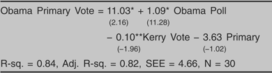
The foregoing gives us three possible correction values for our Equation 3 forecast of 56.57% of the two-party vote for Obama: 0.77, 0.87, and 0.90. If we simply multiply the Equation 3 forecast by each of these proportions, respectively, we arrive at the following revised estimates for the Obama share: 43.6%, 49.2%, and 50.9%. Which is more likely? To help answer that question, we combine information from the above polling data and the primary voting data (Kerry and Obama), to formulate and estimate (OLS) a model of the Obama vote, shown here in Equation 4.

Table 4.

Equation 4: Obama Primary Vote Model

Notes: Obama primary vote = the percentage of the state Democratic primary vote received by Obama; Obama poll = the average percentage support in the last pre-primary polls in the state; Kerry vote = the percentage of the state Democratic primary vote received by Kerry in 2004; Primary = 1 if primary contest, 0 if caucus contest); the statistics are defined as with Equation 2, and ** = statistical significance at 0.10, two-tail; N = 30 states.

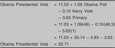
The results from Equation 4 confirm our earlier finding of no Bradley effect in the Democratic primaries, i.e., a 1-point increase in Obama's poll numbers leads to a 1-point increase in his vote. Further, the Kerry vote is a significant predictor of the Obama vote. Finally, the coefficient for the primary dummy has the expected sign, although it falls short of conventional significance levels. (The expectation was that Obama would do better in caucus states where voters could not express racist leanings in the privacy of a voting booth.) In sum, the model accounts rather well for the Obama vote, as expressed in the 2008 Democratic primaries. For heuristic purposes, we now make the bold assumption that the 2008 presidential contest in November replicates, in its parameters, the structure of Equation 4, using that model to provide an alternative 2008 forecast, shown here as Equation 5.

If the estimate of Equation 5 is correct, then the adjustment to our original model forecast involves a correction of something like .93 (i.e., 52.71/56.81 = 0.93). Including this correction, we now have explored four possible correction values: 0.77, 0.87, 0.90, and 0.93. We return to these choices, and a final consideration, in the conclusion.

Table 5.

Equation 5

Notes: Obama presidential vote = the estimated two-party popular vote share in the 2008 presidential contest; Obama Poll score = 46 = the national Gallup vote intention trialheat share for Obama in June; Kerry Vote score = 48.3 = the national popular vote share for Kerry in 2004; Primary score = 1 = popular vote contest rather than caucus contest.

In the meantime, Equation 5, and its forecast, may not be far-fetched. It is based overwhelmingly on the close empirical link we established between Obama state opinion poll performance and Obama vote performance in the primaries. Will national opinion polls predict national vote as well? Gallup and Rasmussen tracking polls over the months of June and July gave Obama a 4–6 point margin, on average (Abramowitz, Mann, and Sabato Reference Abramowitz, Mann and Sabato2008). The Equation 5 forecast falls within this range, predicting an Obama lead of 5.4 points over McCain. Of course, the critical question regards the accuracy of these mid-summer polls. (Their historical inaccuracy is a principal reason scholars such as ourselves forsook this vote intention approach to forecasting.) The correlation between the “trial-heat” items and the two-party popular vote, respectively, for June and July are 0.65 and 0.79 (Abramowitz Reference Abramowitz2008; Campbell Reference Campbell2008). Interestingly, the Pollyvote web site (http://www.pollyvote.com), which forecasts a presidential election by averaging competing methodologies (polls, expert surveys, Iowa Electronic Market, quantitative models), makes a July 21 forecast of 52% for Obama, very close to the 52.71% forecast of Equation 5.

Summary and Conclusion

Our Jobs Model forecasts that the Republicans, now incumbent in the White House, will experience a shattering defeat, indeed the greatest incumbent popular vote loss on record from 1948, garnering just 43.4% of the two-party popular vote. How accurate is this forecast? Consider simple statistical error. The standard error of estimate is 1.4; but adding even three times that amount to the point forecast would still predict a clear Republican loss (at 47.7%). Put another way, if Obama receives less than 50% of the popular vote, the Jobs Model would have registered an error of over 6.6 points. That would be the largest out-of-sample error in the data-set. It implies that there is less than a 1 in 14 chance that the model is wrong in forecasting an Obama victory.

Nevertheless, the Jobs Model is not a “shoo-in” for Obama, once ballot box racism is taken into account. By various estimates, Obama will lose a chunk of votes because he is Black, rather than White. This seems unavoidable. In the foregoing, we evaluated four possible correction values: 0.77, 0.87, 0.90, and 0.93. Which is closer to the truth? In order to avoid appearing arbitrary, we simply take the median of these four values (0.885) as the proportion of voters who will not take race itself into account. By that reckoning, Obama would win in a close contest (i.e., a 0.885 correction to the Jobs Model predicts an Obama two-party popular vote forecast of 50.1%).Footnote ³ But if the correction number is lower, by even a small amount, he could well lose. In any event, we expect the competition to be much closer than what is implied by our original, uncorrected Jobs Model.