2. Observations

For this paper, we make use of two types of data. The first are archival calibration observations that were primarily taken for pulsar observing projects. These files are folded observations of a pulsed noise source, which were taken in order to calibrate subsequent pulsar observations. These range from a few very short (few second duration) observations to one observed for almost 20 min. However, by far the majority had a duration of 2 min. These data files are in psrfits (Hotan et al. Reference Hotan, van Straten and Manchester2004) fold-mode data format, typically have 1 MHz frequency resolution and are integrated over a few minutes. We have chosen to make use of these files as (1) they are relatively small in volume and hence quick and easy to process and (2) provide almost daily snap-shots of the RFI environment over the entire band since the early observations with the receiver. We process these data using the pfits and psrchive software suites. Specifically we time- and polarisation- average using pam and then process the dat_offs and dat_scls psrfits tables in pfits_formBandpass to determine the averaged spectral bandpass throughout the calibration observation.

We record the meta-data (e.g. observation time and pointing direction) along with each spectrum and hence can determine the average signal strength in part of the band as a function of date, time-of-day, telescope Azimuth and Zenith, equatorial coordinates etc. While we do not calibrate into physical units, we do account for known large-scale attenuation changes caused by the addition (or subtraction) of attenuator physical components into the signal chain. All these observations are publicly available from the CSIRO Data Archive.Footnote ^a

It is not possible to use the calibration observations described above to test and demonstrate mitigation algorithms because they have been folded at the period of the switching noise source and channelised using a 2 048-pt transform before summing the resulting powers of the two polarisation states into 1 MHz channels. We therefore have also recorded a 16-bit voltage data stream of our UWL subband of interest. During this 10 s observation, taken on 10 August 2023 at UTC 02:41:26, the telescope was observing the bright pulsar PSR J0835 $-$ 4510 (also known as the Vela pulsar) and the corresponding data file was 10 GB in volume. Vela was chosen as it is the brightest known pulsar and we can detect individual pulses from this pulsar in our 10 s test data set. As most of our mitigation methods are based on thresholding we can use this observation to demonstrate that we can remove bright RFI, without removing the bright astronomical signal (and noting that other pulsars will be weaker and hence even less affected by thresholding rejection methods). The corresponding data file is stored in the dada format as offset binary encoding, 2 polarisation states interleaved in blocks of 2 048 voltage samples. Such data can be processed using the dspsr software (van Straten & Bailes Reference van Straten and Bailes2011), but we have also developed our own code (in C, Python and GnuRadio) for analysing these data.

3. Band integrated and long-term RFI characterisation

Even though Murriyang is not designed as a WiFi and Bluetooth receiver, and cannot point directly to the horizon (where the majority of these terrestrial signals originate), the RFI picked up in the side lobes do still impact observations. A typical Bluetooth transmitter outputs between 2.5 and 100 mW (Anees Reference Anees2024). If in the primary beam of the telescope (assuming 1 s integrations), such a signal could be detected from a range of $\simeq$ 83 000–520 000 km. Given the telescope’s focus cabin height of 58 m, the line of sight to the radio horizon is approximately 27.2 km. This places the town of Parkes, located 17.8 km away, well within range, and thus a potential source of RFI.

However, Murriyang has an elevation limit of 30.25 degrees and hence the signals from Parkes will be detected through the far side-lobes. In the far side-lobes with a gain of 0 dBi, the range a Bluetooth signal could be detected is reduced to $\simeq$ 7 300–46 500 km. The strongest individual signals are strongly correlated with the operating hours of the visitors’ centre (which typically receives up to around 100 000 visitors per year), from our own laboratories and on-site offices, and from the local farming community.

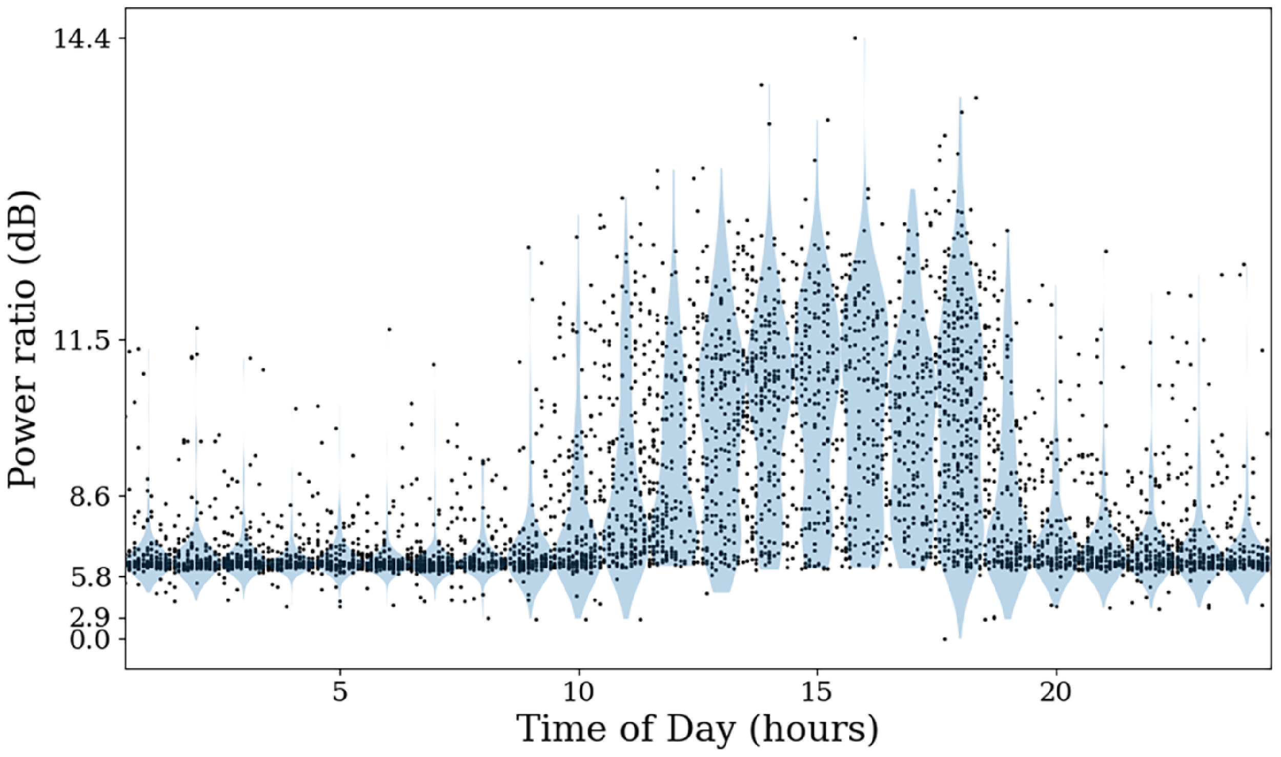
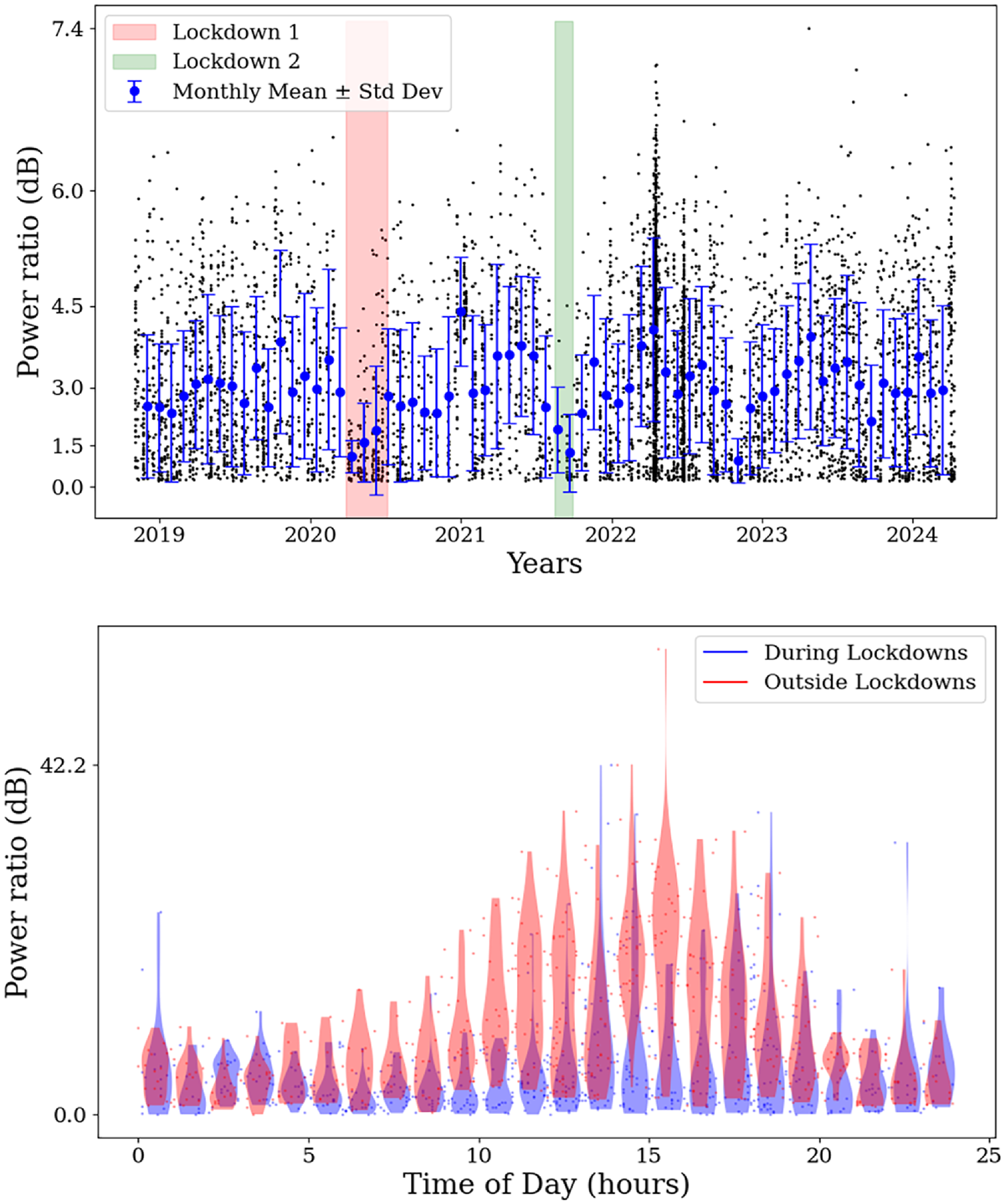
To investigate the origin of the 2 432 MHz subband RFI in greater detail, we analysed the archival calibrator observations by computing the average power across the subband as a function of time and pointing direction. As shown in Figure 1, there is a clear increase in received power during typical Australian business hours (9am–5pm). There was also a noticeable decrease in the intensity of RFI during periods when the Parkes telescope visitor centre and on-site offices were closed due to local COVID lockdowns. These can be seen in Figure 2, but even during such lockdowns some observations were affected by RFI suggesting, as expected, that not all the RFI originates from a single place. The lower panel in Figure 2 shows the decrease in power received during the first lockdown period. Note that this panel includes all data obtained during the specific time periods, whereas the top panel (and other related Figures) uses a restricted elevation angle from 40 $^{\circ}$ to 60 $^{\circ}$ .

Figure 1.

Violin plot showing the total measured power in the 2 432 MHz subband (as a ratio of the minimum power recorded) as a function of time of day, extracted from calibrator data files taken over the period of 5 years. It shows a distinct increase in the RFI around standard Australian business hours 9am–5pm.

Figure 2.

The top panel shows signal strength received in the 2 432 MHz subband (as a ratio of the minimum power recorded) over a period of 5 years, over a restricted elevation angle of 40 $^{\circ}$ –60 $^{\circ}$ . The Parkes Telescope visitor centre was closed due to lockdowns from the 27th March to 4th July 2020 (Lockdown 1) and 15 August to 27 September 2021 (Lockdown 2). The circles show the monthly mean received signal strength, as extracted from calibrator data files taken over the period of 5 years, with the bars showing $\pm$ 1 standard deviation. The coloured bars show the period of the lockdowns and a noticeable decrease in the intensity of the monthly mean of the RFI. The lower panel shows the comparison in power as a function of time of day, this time comparing the power during the first lockdown (April–June 2020) and the power from an equivalent date range outside of the lock-down period (April–June 2023). For this panel, we did not constrain the elevation angle to ensure an adequate number of observations for comparison.

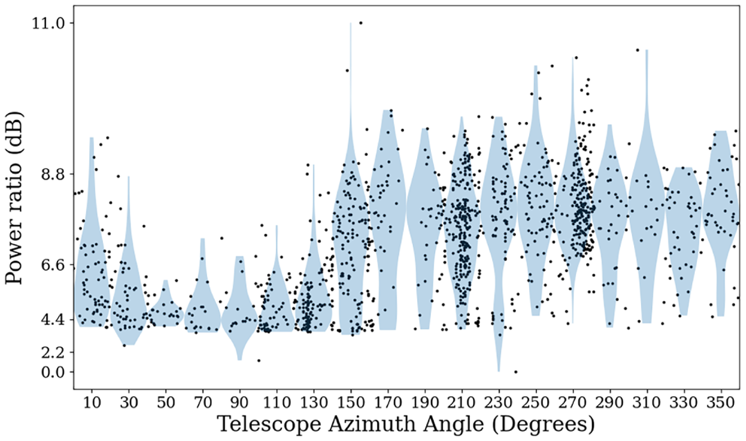
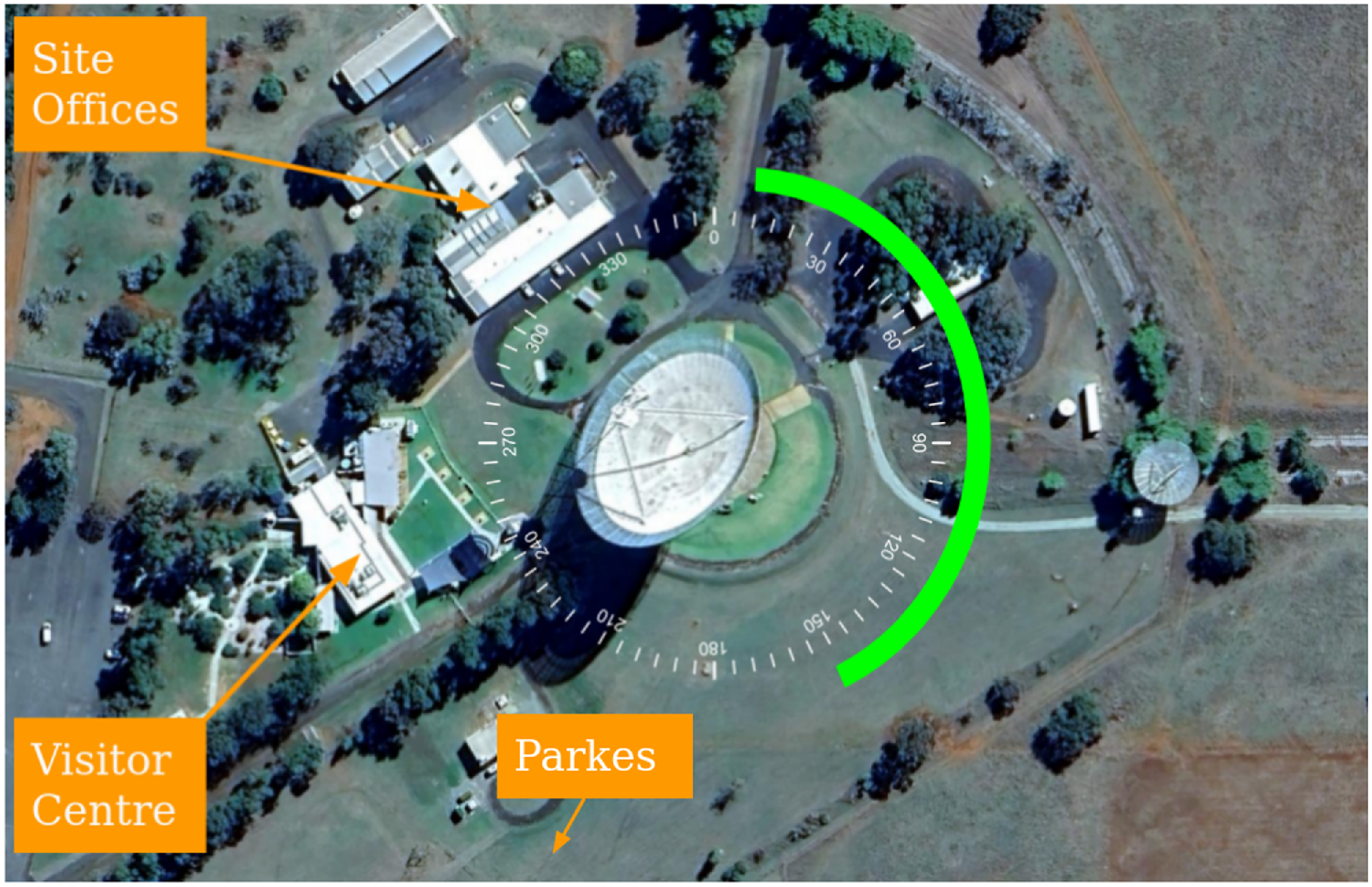
As shown in Figure 3, the RFI signal strength in the WiFi/Bluetooth bands shows a distinct directional bias to the West, which is in the direction of the town of Parkes, the Parkes Observatory Visitor Centre and Site Offices. Figure 4 shows a satellite image of the location of the various buildings and telescope on the observatory site. A noticeable drop in the power of the RFI received by the telescope can be seen from the angles E 40 $^{\circ}$ to E 140 $^{\circ}$ while conversely an increase in the power received can be seen between the angles of W 150 $^{\circ}$ to W 360 $^{\circ}$ . This is likely due to the 64 m reflector screening the prime focus from the RFI source and provides additional evidence that the likely culprits for the sources of RFI are the visitors centre, site offices and/or Parkes.

Figure 3.

Signal strength received by the telescope in the 2 432 MHz subband (as a ratio of the minimum power recorded) as a function of direction (in $20^\circ$ intervals), extracted from calibrator data files taken over the period of 5 years. This shows a significant, direction-dependent variation in power received, with significant increases to the West and relatively low levels in the range from 40–140 degrees E.

Figure 4.

Satellite image of the Parkes telescope site. The compass centred in the telescope shows that the location of the visitor centre (marked) is to the West of the telescope at W 240 $^{\circ}$ –W 275 $^{\circ}$ and the site office building is located between W 290 $^{\circ}$ and W 340 $^{\circ}$ . The green bar shows the range of angles from Figure 3 with the lowest received signal strength (Image: Google Earth).

Even though visitors to the Parkes Observatory site are asked to switch off their Bluetooth and WiFi-enabled devices, it is clear that many do not do so. Visitors may also be setting their phones to Flight Mode in good faith, unaware that on newer mobile handsets this no longer automatically disables Bluetooth and Wifi. In some instances, they may turn off a primary device (e.g. a phone) but not a secondary device (e.g. smart watch), which may result in the secondary device continuing to advertise and probe for connection. Noting that such devices are now ubiquitous, it is unrealistic to expect a pristine, RFI-free, site next to a visitor centre. For observations which require clean 2.4 GHz observations, night-time observations are less affected. However, as we will show below, we can recover much of the astronomical signal in this band even during the day-time.

4. Temporal and frequency resolved RFI characterisation

RFI caused by WiFi and Bluetooth should be characterised by their well-defined protocols. In the 2.4 GHz band, the most common Wireless Local Area Network (WLAN) standard used today is the IEEE 802.11 family, specifically 802.11 and 802.11b/g/n/ax. This WiFi band runs from 2.401 to 2.4835 GHz and is divided into 13 channels in Australia. Each channel is spaced 5 MHz apart. The channel width depends on the signalling method, with Direct Sequence Spread Spectrum (DSSS) using 22 MHz wide channels and Orthogonal Frequency-Division Multiplexing (OFDM) using 20 MHz wide channels. This results in 11 overlapping channels, with only three non-overlapping channels usable at once, usually channels 1, 6, and 11.

The maximum length of a WiFi packet is 2 304 bytes plus encryption. Depending on the encryption protocol this could add 8–20 bytes to this length resulting in maximum total package lengths of 2 312–2 324 bytes. The bit rate for WiFi varies with the generation, with ‘WiFi-0’ having a bit rate of 1–2 Mbps and ‘WiFi-7’ (the latest available protocol) having a theoretical bit rate of 46 Gbps. This results in a possible packet length of 2 324 $\unicode{x03BC}$ s for ‘WiFi-0’ and as short as 0.05052 $\unicode{x03BC}$ s for ‘WiFi-7’.

With the proliferation of Bluetooth connectable technology available today, the RFI is no longer limited to mobile phone handsets, but also includes wearable devices such as watches and fitness monitors, and also cars. Bluetooth transmits in one of two fashions: (1) the Basic Rate/Enhanced Data Rate (BR/EDR; also called Classic Bluetooth) which uses 79 $\times$ 1 MHz channels and (2) the Low Energy (LE; or BLE) which uses 40 $\times$ 2 MHz channels.Footnote ^b Both methods use frequency hopping to transmit data, switching channels pseudo-randomly 1 600 times per second in a connected state and 3 200 times per second in an inquiring state, resulting in packet lengths of 312–625 $\unicode{x03BC}$ s. This frequency hopping reduces signal interference with other Bluetooth signals in this highly used unlicensed portion of the ISM band, but can interfere with WiFi channels. Compared to WiFi, Bluetooth is short-ranged and used to establish Personal Area Networks (PAN) that are limited to 100 m for Class 1 Bluetooth devices and 30–40 m for Class 2 Bluetooth devices (generally available in commercial devices such as phones).

Bluetooth Low Energy advertising channels are used by devices to establish connections with other devices. There are three Primary Advertising Channels that are selected to minimise interference to the primary WiFi data channels. The three channels are Channel 37 centred on 2 402 MHz, Channel 38 centred on 2 426 MHz, and Channel 39 centred on 2 480 MHz. Advertising data is transmitted simultaneously on all three channels to increase the probability of receipt. Since all devices using Bluetooth Low Energy advertise for connection on the same three advertising channels, these channels usually contain a major part of the Bluetooth RFI. This also indicates the predominance of Bluetooth RFI appears to be coming from devices using the LE protocol.

4.1 Demodulating the Bluetooth signal

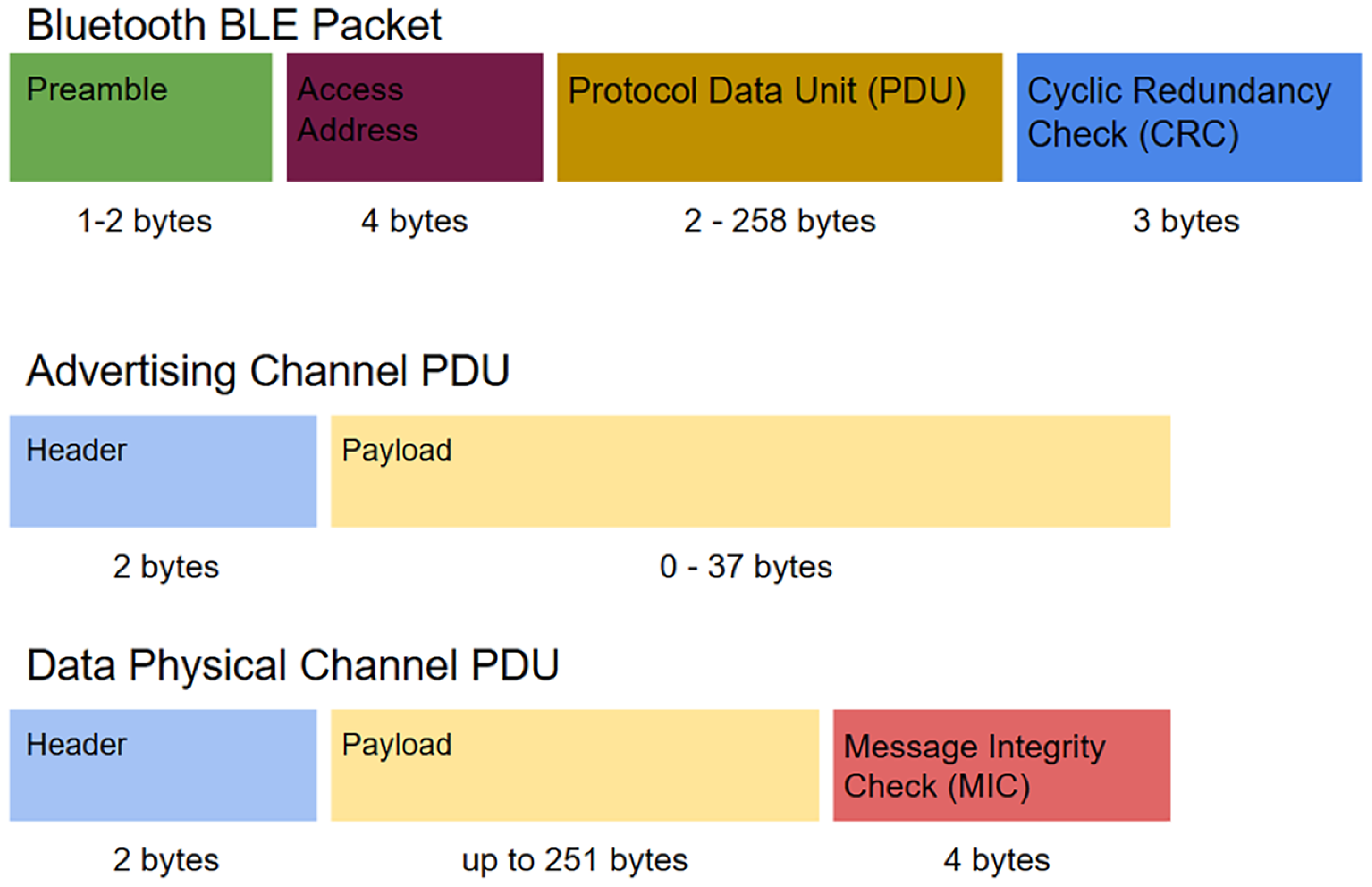
Bluetooth uses a Gaussian Frequency Shift (GFSK) modulation scheme to convert each channel’s carrier frequency to transfer binary information. This is done by modulating the carrier frequency by at least $\pm185$ KHz with an increase representing a 1 (mark) and a decrease representing a 0 (space) (Anees Reference Anees2024). Each Bluetooth packet is made up of four distinct parts: a preamble, access address, Protocol Data Unit (PDU) and a Cyclic Redundancy Check (CRC), see Figure 5. The PDU of the packet will differ based on whether the device is requesting a connection on an advertising channel or in a connected state and transferring data (see Figure 5). Regardless, the preamble of a packet is a string of alternating 1s and 0s whose purpose is, among other things, to set the symbol timing estimation which essentially informs the receiver of the bit rate transmission.

Figure 5.

The structure of different Bluetooth packets. At top is the whole packet structure, while the lower two parts show the different forms for the Protocol Data Unit (PDU) for the top figure.

The Bluetooth signal packets seen in our recorded data ranged in time from around 288 to 25 000 $\unicode{x03BC}$ s while the WiFi transmissions ranged in time from around 1 200 to 3 500 $\unicode{x03BC}$ s. Even though the Bluetooth protocol allows for transmissions between 312 and 625 $\mu$ s in length, our data shows that the majority of the Bluetooth packets lasts around 288 $\unicode{x03BC} s$ .

Figure 6.

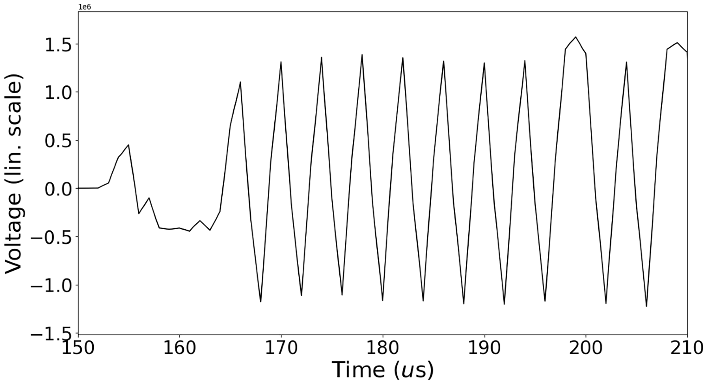
The beginning of a representative Bluetooth advertising packet after the signal has been demodulated. This shows the 2 402 MHz advertising channel (Channel 37) from 150 $\unicode{x03BC}$ s in our data. This shows the bits encoded as Gaussian Frequency Shift Keying from the central frequency. The preamble can be seen by the alternating marks (1s) and spaces (0s).

Figure 7.

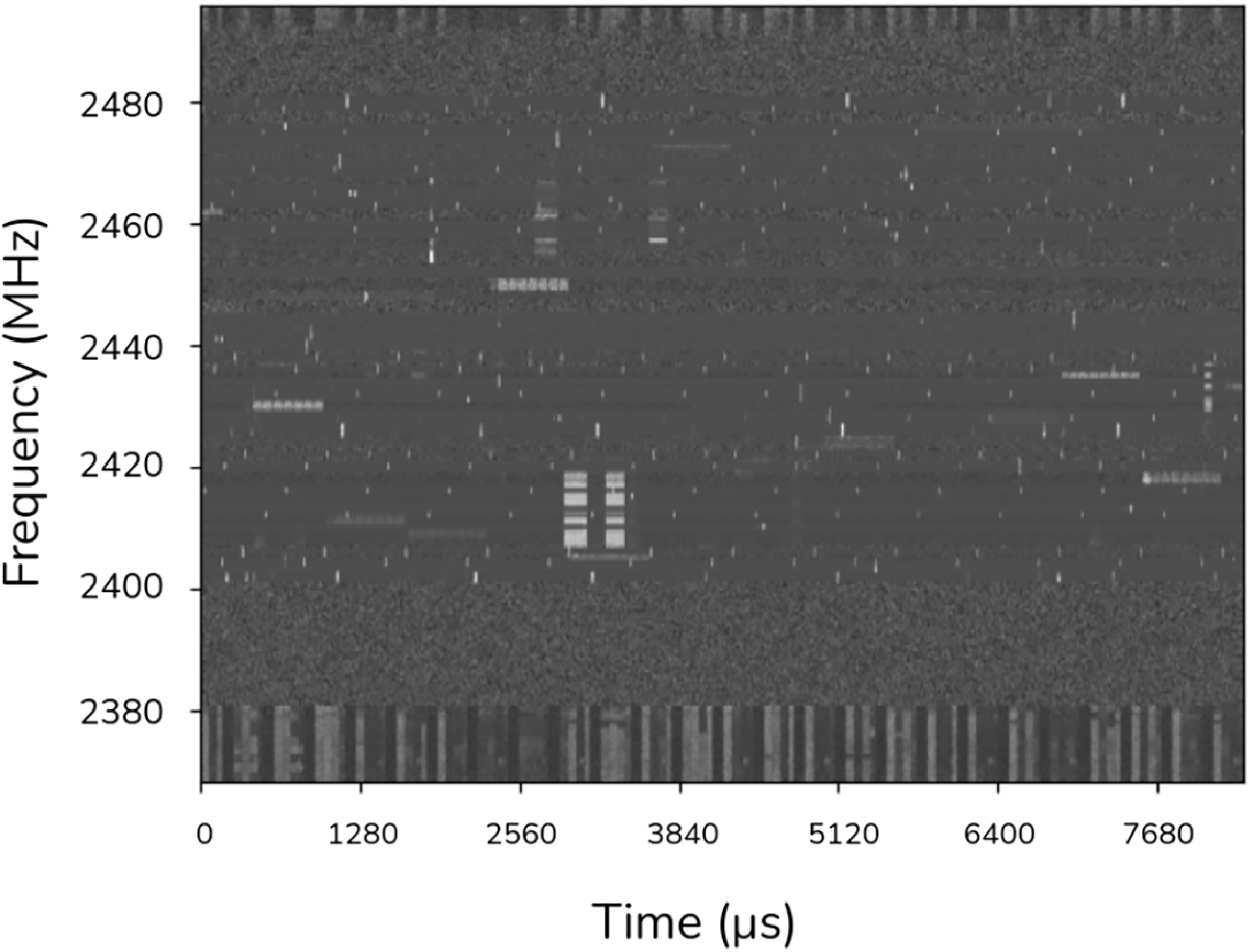
Dynamic spectrum of a 0.5 s sample of the channelised data from our observation. Visible in the data are samples of Bluetooth and Wifi. The narrow frequency band features (horizontal), both shorter and loner time spans, are Bluetooth signals. The intermediate time span signals over broader frequency ranges (vertical) are WiFi signals. The RFI in the lower frequency range is due to NBN and is aliased at the upper edge of the frequency band.

We developed tools to filter the incoming data stream to select a specific Bluetooth channel, identify regions containing transmission and then to demodulate the packet, see Appendix A. The code, working on each individual BLE channel, shifts the Bluetooth frequency channel to baseband, applies a bandwidth Finite Impulse Response (FIR) filter to the signal, downsamples the voltage data to closer to the bit rate of the Bluetooth signals, and finally performs a simple demodulation to obtain bits of information from the carrier frequency. As an example, Figure 6 shows the beginning of a representative demodulated packet with the triangular pattern indicating the 10101010 header information.

4.2 Characterising the components of the Parkes voltage data

WiFi and Bluetooth signals that are significantly brighter than any reasonable expectation for an astronomical signal could potentially be mitigated using a simple thresholding algorithm. In order to explore the relative brightnesses of the RFI, the telescope system, and the bright astronomical source in our test data (the Vela pulsar), we channelised the 10 s voltage data set with high time resolution (microsecond resolution), summed the polarisations and then inspected the resulting time-frequency output by eye. Figure 7 shows the distinct time and frequency signatures of the various RFI packets, the intermediate duration wider frequency RFI being WiFi packets, while the longer narrow frequency packets and the short duration narrow frequency packets are Bluetooth packets. The RFI covering the entire time period at the lower end of the frequency range is due to the NBN, and is also aliased in the upper end of the range. Within our 10 s of data the majority of the RFI appears to come from the BLE advertising channels (but not all; we see Bluetooth transmission across the 2 402–2 480 MHz band). Having demodulated each of the Bluetooth advertising channels, we note that the device addresses being transmitted indicate that the signals are from independent devices searching for other Bluetooth enabled devices.

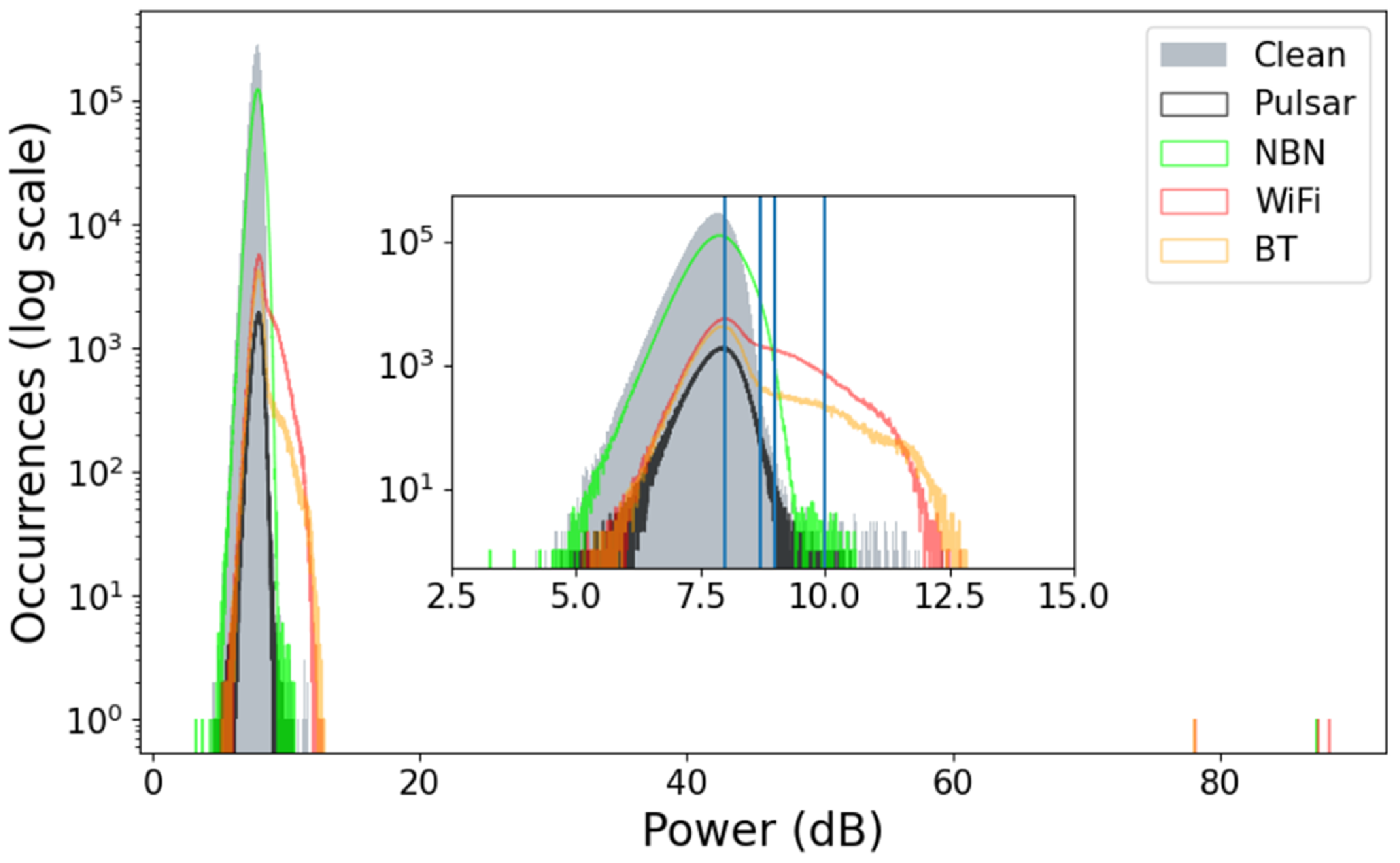
For a representative 1.3 s of data, we manually selected regions that were clearly dominated by the various signals of interest (WiFi, Bluetooth, NBN transmissions, the pulsar and clean parts of the band) and measured the power levels of the samples in each category. The results are shown in Figure 8. Note that this relatively-crude approach of manually selecting data blocks results in the inclusion of clean data in each RFI category, but is still informative. The RFI ranges in power from the level of the astronomical signal to orders of magnitudes higher.

Figure 8.

Histogram showing the number of samples received as a function of power in the the 2 432 MHz subband in the channelised time series. Both the x and y axes are on a log scale. Colours show some of the elements in 1.3 s of the channelised data including clean signal in solid grey, the pulsar signal in black, the NBN RFI in green, WiFi RFI in orange and Bluetooth RFI in yellow. As described in the text, all categories contain significant ‘contamination’ from clean samples, but the characteristic power levels of the brightest RFI can still be seen. The blue lines represent the voltage thresholds that were tested at 8, 8.69, 9 and 10 dB in Section 5.2.

We also note that the power levels are obtained from microsecond time resolution and hence include very short, very bright bursts of RFI.Footnote ^c

Clearly the very brightest WiFi and Bluetooth signals could be removed with a simple thresholding algorithm with no loss of astronomical data. However, more care is needed to distinguish the weaker RFI from astronomical signals.

5. Mitigation

In the standard astronomical data products available from the Parkes observatory (such as folding the data stream at the known period of a pulsar or calibrator, observing with high spectral resolution or with high time resolution), it is not currently possible to mitigate the Bluetooth and WiFi signals without simply flagging the majority of the band and hence losing the astronomical signal entirely in that band.

The primary receiver currently installed on the Parkes telescope is a single pixel feed, and hence we cannot use mitigation methods such as beam nulling (Fridman & Baan Reference Fridman and Baan2001). We also do not have a fully implemented system to apply mitigation methods that rely on a reference antenna(Kesteven et al. Reference Kesteven2005).

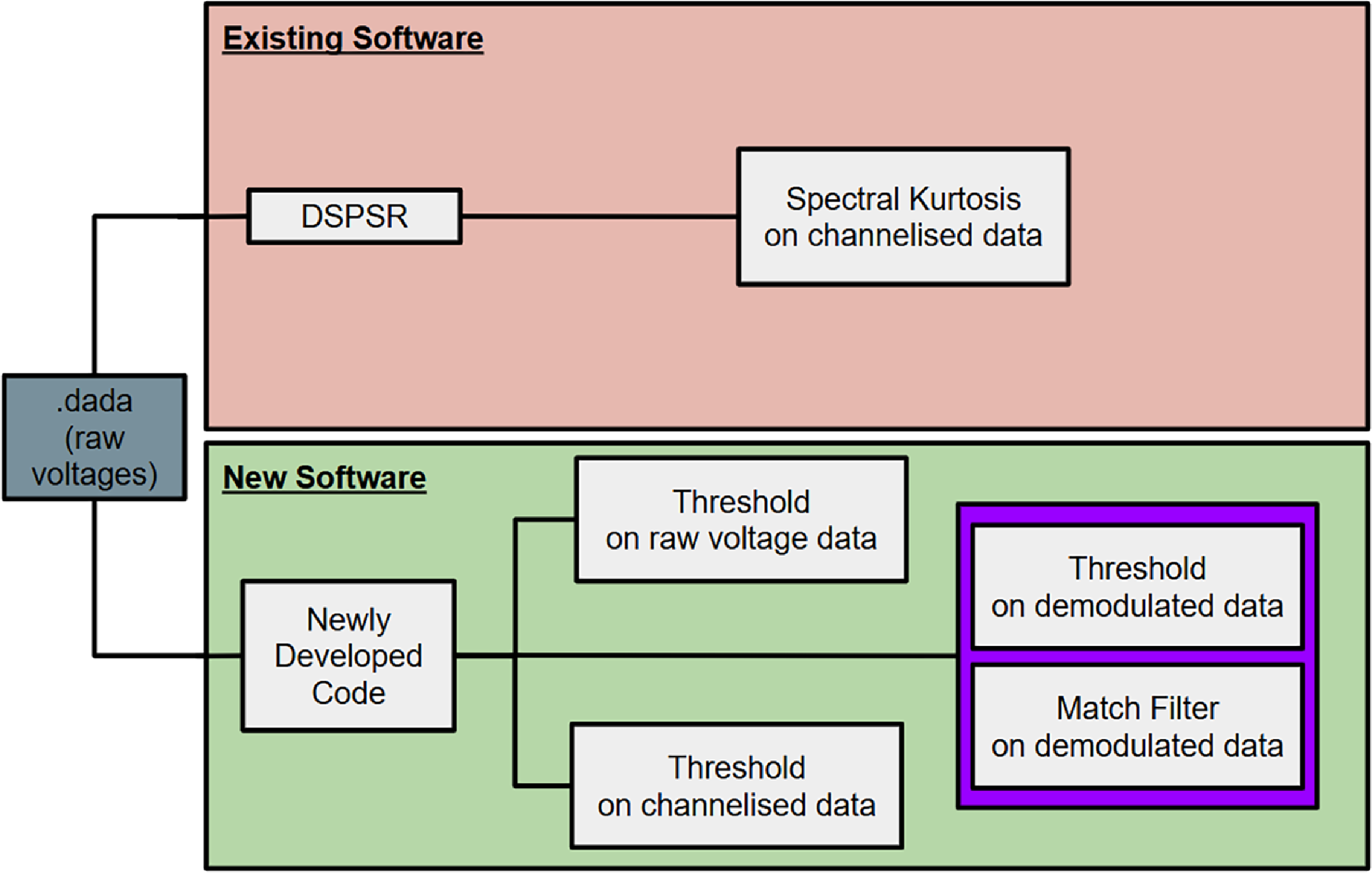
We therefore have to rely on software methods for mitigation of the processed data products. There are two general avenues for this approach: (1) use existing software for RFI mitigation or (2) develop new software. The existing software package used for real-time processing of data from the Parkes Telescope is DSPSR. DSPSR uses spectral kurtosis for the mitigation of RFI in data that is folded at the period of a known pulsar or calibrator. Our newly developed software package implements a number of other methods. Both DSPSR and the new package take voltage data streams as inputs, apply the mitigation algorithms and output astronomical data products. The range of existing and newly-developed options tested in this work are represented in the flowchart shown in Figure 9.

Figure 9.

Flowchart depicting general methods to approach the processing of the raw voltage data from Parkes observations. The Existing Software avenue includes the software package DSPSR and uses spectral kurtosis as the RFI mitigation method. Our new method uses software that mitigates RFI by applying a threshold to the channelised data, as well as applying filters to demodulated data streams.

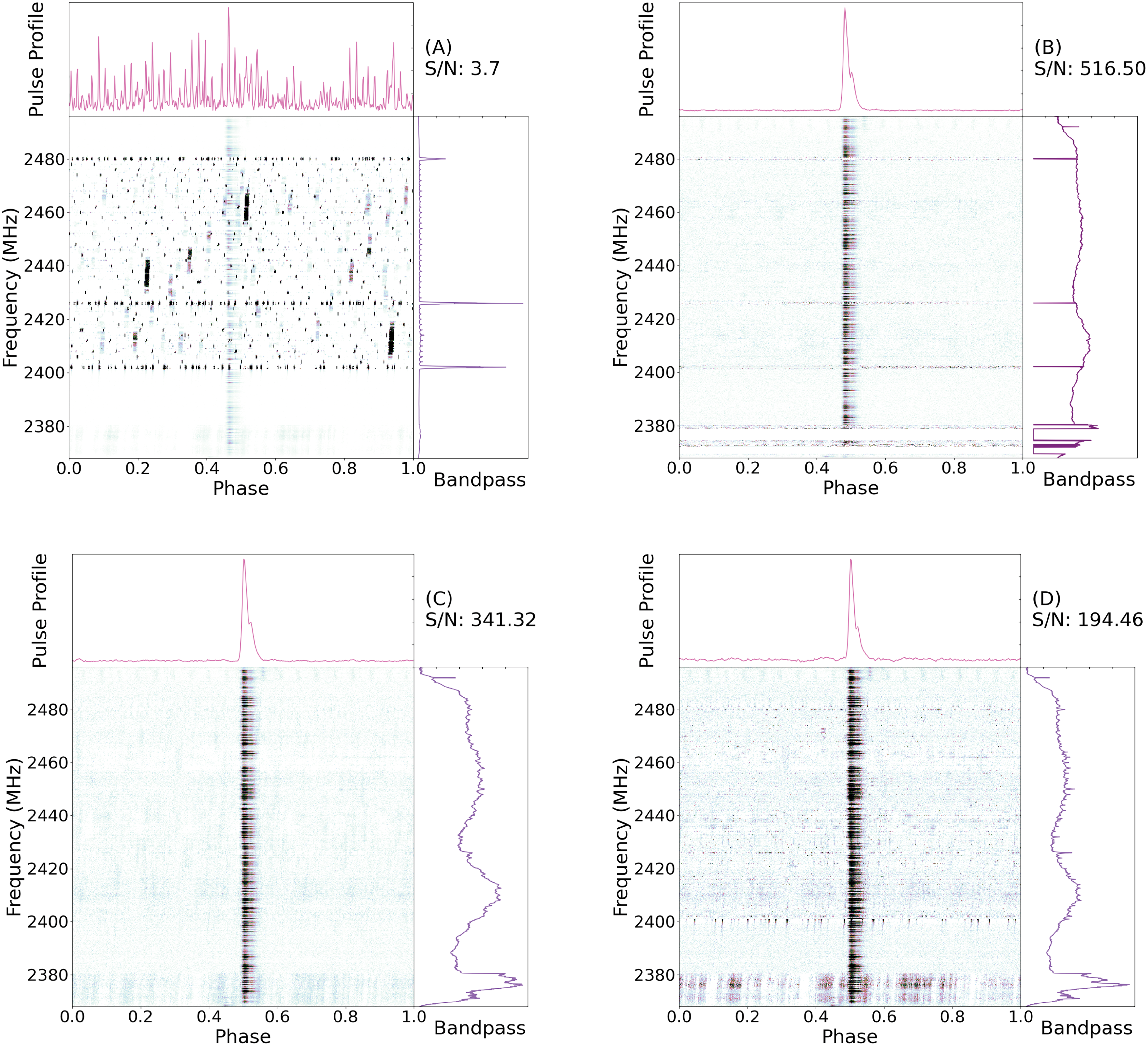
Throughout the following, we compare the effectiveness of the various mitigation methods by folding the full 10 s RFI-mitigated voltage data stream at the period of the Vela pulsar and measuring the resulting S/N of the pulse profile. We also display the folded pulse profile, phase-frequency diagram of the pulse profile, and the averaged (in time) frequency spectrum for all methods in Figure 10. For comparison purposes, Figure 10(A) shows the pulse profile without any mitigation (top panel). The pulse in this Figure is undetectable. The right-hand panel of the same figure shows the time-averaged bandpass with the three primary features being the Bluetooth advertising channels. The central panel shows the de-dispersed pulse profile in a frequency-phase plot. To indicate that the Vela pulsar is present we have had to choose a colour-scale in which the RFI is saturated. The S/N is determined as the sum of the pulse profile (with prior knowledge of the phase of the pulse) divided by the standard deviation of the baseline. In this case the S/N value is dominated by the RFI.

Figure 10.

The result of various mitigation methods. The power levels have been normalised. (A) The full 10 s of channelised data with no RFI-mitigation applied. The dynamic spectrum is overpowered by the RFI. There is no discernible pulse profile and bandpass in dominated by powerful channelised RFI. (B) The folded dynamic spectra, pulse profile and bandpass with the default DSPSR spectral kurtosis settings ( $N_{\sigma}$ ( $\sigma$ ) = 4.1; N = 2 688; with no time or freq. scrunching) implemented. (C) The 10 s of data after a 8.69 dB power threshold has been applied. As a result there is a prominent pulse visible in the dynamic spectrum. There is also a visible pulse profile and relatively smooth bandpass present. (D) The application of a combination of the averaged power threshold and the simple threshold on the demodulated data.

Figure 10. Long description

Panel A: A dynamic spectrum plot with no RFI mitigation applied. The x-axis represents phase ranging from 0.0 to 1.0, and the y-axis represents frequency in MHz from 2380 to 2480. The pulse profile at the top shows no discernible pulse, and the bandpass on the right is dominated by powerful channelized RFI. Panel B: A dynamic spectrum plot with default DSPSR spectral kurtosis settings applied. The x-axis represents phase ranging from 0.0 to 1.0, and the y-axis represents frequency in MHz from 2380 to 2480. The pulse profile at the top shows a clear pulse, and the bandpass on the right is relatively smooth. Panel C: A dynamic spectrum plot after applying an 8.69 dB power threshold. The x-axis represents phase ranging from 0.0 to 1.0, and the y-axis represents frequency in MHz from 2380 to 2480. The pulse profile at the top shows a prominent pulse, and the bandpass on the right is relatively smooth. Panel D: A dynamic spectrum plot with a combination of averaged power threshold and simple threshold on the demodulated data. The x-axis represents phase ranging from 0.0 to 1.0, and the y-axis represents frequency in MHz from 2380 to 2480. The pulse profile at the top shows a clear pulse, and the bandpass on the right is relatively smooth.

5.1 Spectral kurtosis

As a spectral kurtosis method is readily available via the DSPSR package, we demonstrate the effectiveness of this method first.Footnote ^d Spectral kurtosis ( $\widehat{SK}$ ) is the spectral variant of time-domain kurtosis (Dwyer Reference Dwyer1984; Vrabie et al. Reference Vrabie, Granjon and Serviere2003; Nita et al. Reference Nita, Gary, Liu, Hurford and White2007; Nita & Gary Reference Nita and Gary2010). Time-domain kurtosis measures the fourth statistical moment of a signal’s amplitude distribution to quantify its deviation from Gaussianity, and is commonly used for detecting transient acoustic events or diagnosing mechanical faults. In contrast, spectral kurtosis characterises the non-Gaussianity of signal power as a function of frequency, enabling the detection of impulsive or transient features in the spectrum. This property makes it a powerful and widely used tool for identifying radio frequency interference (RFI) in radio astronomy data.

DSPSR processes the raw voltage data by channelising it and then converting the signal to a detected power. The $\widehat{SK}$ estimator is computed from blocks of this detected power data to estimate its non-Gaussianity and determine whether to excise it. Since most RFI exhibits non-Gaussian statistics, with power values skewed to higher levels, the $\widehat{SK}$ estimator can identify regions affected by interference (Nita et al. Reference Nita, Gary, Liu, Hurford and White2007).

The key input parameters for the DSPSR spectral kurtosis algorithm are the number of samples (N) used to compute the statistical estimates, and the threshold, expressed in units of standard deviations ( $\sigma$ ), that determines whether a block of samples should be excised.

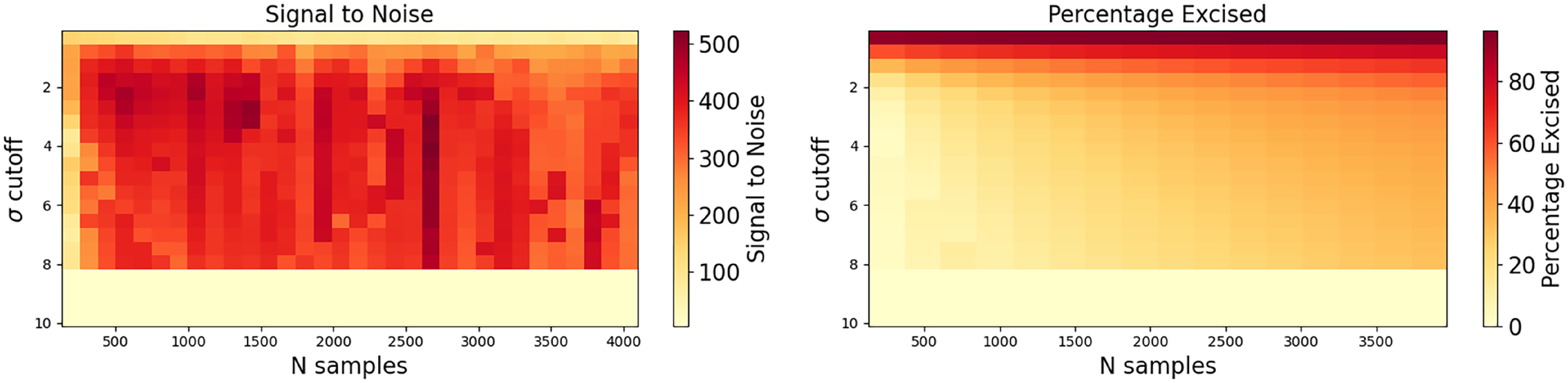
We applied the kurtosis method with a range of trial parameters on our 10-s voltage data stream. To compare the effectiveness of the algorithm we channelised the data into 2 048 channels (note that this gives us a sample resolution of 62.5 ms) and folded at the period of Vela with 512 bins. We then measured the signal-to-noise of the resulting pulse profile and obtained the percentage of the 10 s data that was removed. The results are shown in Figure 11.Footnote ^e In all cases the S/N of the pulse profile significantly exceeds that obtained with no mitigation applied. Comparing Figure 10(A) with (B) shows that this mitigation method allows the Vela pulsar to be easily detected with high S/N. This figure was obtained with 2 048 frequency channels and processed with the parameters that give the maximum S/N (516) in Figure 11, obtained with a sample size of 2 688 and a sigma threshold of 4.1. We note that this performance significantly exceeds that of the current DSPSR default settings ( $N=128$ ; $\sigma=3$ ), with a S/N in these trials of 121.

Figure 11.

Heat maps comparing the signal to noise ratios and percentage of data excised for the pulse profile output of DSPSR. Each frame shows the effect of varying the number of samples N and the threshold for excision $\sigma$ used for calculating spectral kurtosis of RFI. These were calculated using 2 048 frequency channels.

5.2 Simple power threshold

The simplest mitigation method is simply to inspect the 16-bit voltage data stream and skip blocks of data where the data values exceeds a given threshold. However, as the RFI signal hops in frequency we can significantly improve the algorithm by searching for strong signals in the known WiFi and Bluetooth bands after channelising and detecting the signal. For a given frequency channel, signals above a specified power threshold are then not included when binning the pulse profile.

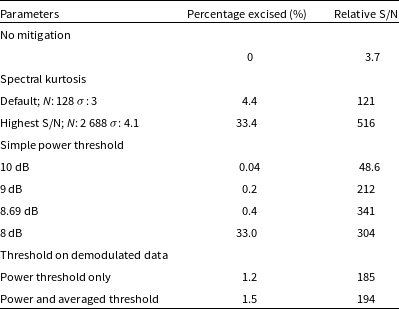
We tested several power thresholds (10, 9, 8.69, and 8 dB) defined as the ratio of the power to the minimum total power in the channelised data. The results are shown in Table 1. The folded pulse profile obtained using the highest S/N set of parameters is shown in Figure 10(C). We note that the resulting S/N of the profile is high and yet we only excise 0.4% of the data (significantly less than the kurtosis method). The reduction in S/N of the pulse profile using this method compared to the spectral kurtosis is because low-level interference remains and hence the noise level of the baseline is larger in this scenario.

Table 1.

This table compares the percentage of excised data and the relative signal to noise ratio for different mitigation methods tested.

Table 1. Long description

The table has 6 rows and 3 columns. The columns are labeled Parameters, Percentage excised (%), and Relative S/N. The rows are labeled with different mitigation methods and their corresponding values. Row 1: No mitigation, 0, 3.7. Row 2: Spectral kurtosis Default; N: 128 σ: 3, 4.4, 121. Row 3: Spectral kurtosis Highest S/N; N: 2 688 σ: 4.1, 33.4, 516. Row 4: Simple power threshold 10 dB, 0.04, 48.6. Row 5: Simple power threshold 9 dB, 0.2, 212. Row 6: Simple power threshold 8.69 dB, 0.4, 341. Row 7: Simple power threshold 8 dB, 33.0, 304. Row 8: Threshold on demodulated data Power threshold only, 1.2, 185. Row 9: Threshold on demodulated data Power and averaged threshold, 1.5, 194.