2.1 Characteristic scales

CSF is an incompressible Newtonian fluid with density $\unicode[STIX]{x1D70C}$ and kinematic viscosity $\unicode[STIX]{x1D708}$ similar to those of water. It fills the subarachnoid space of the spinal canal, a thin annular gap surrounding the spinal cord bounded internally by the pia mater and externally by the deformable dura membrane, as indicated in figure 1(d). The spinal canal is doubly slender, in that its length $L\sim 60{-}80~\text{cm}$ , characteristic perimeter $\ell _{c}\sim 2~\text{cm}$ and characteristic width $h_{c}\sim 0.2~\text{cm}$ satisfy the inequalities

(2.1) $$\begin{eqnarray}L\gg \ell _{c}\gg h_{c}.\end{eqnarray}$$

The associated total volume of CSF in the spinal canal is of the order of $V\sim L\ell _{c}h_{c}\sim 40{-}60~\text{cm}^{3}$ .

The fluctuating motion of CSF in and out of the spinal canal is associated with the periodic variation of the intracranial pressure, driven by the pulsating blood flow in the rigid cranial vault, of angular frequency $\unicode[STIX]{x1D714}$ . In addition to the pulsation associated with the arterial blood flow, it has also been observed in many radiological studies (Kao et al. Reference Kao, Guo, Liou, Hsiao and Chou2008; Dreha-Kulaczewski et al. Reference Dreha-Kulaczewski, Joseph, Merboldt, Ludwig, Gärtner and Frahm2015) that respiration also produces a modulation of the intracranial pressure, resulting in a smaller additional oscillation of the CSF in the spinal canal at a lower frequency (12–18 cycles per minute in adults). For simplicity and reduced complexity of the algebraic manipulations, our analysis assumes the cranial pressure to be a periodic function with angular frequency $\unicode[STIX]{x1D714}$ , equal to that of that of the cardiac cycle. The effects of the lower-frequency component associated with respiratory effects should be addressed in future work by considering a more general temporal variation of the intracranial pressure.

Because of the limited compliance of the spinal canal, measured by the small parameter $\unicode[STIX]{x1D700}$ defined in (1.1), the tidal volume that is displaced along the canal during each cardiac cycle, $\unicode[STIX]{x0394}V\simeq \unicode[STIX]{x1D700}V\simeq 1{-}2~\text{cm}^{3}$ , is much smaller than $V$ . Correspondingly, the periodic flow involves axial displacements of order $\unicode[STIX]{x1D700}L$ in times of order $\unicode[STIX]{x1D714}^{-1}$ , resulting in streamwise velocities of the CSF with characteristic values $u_{c}=\unicode[STIX]{x1D700}\unicode[STIX]{x1D714}L$ of the order of a few $\text{cm}~\text{s}^{-1}$ near the entrance, progressively decaying along the canal to vanish at its closed-end sacral region. The corresponding characteristic values of the azimuthal $w_{c}=\unicode[STIX]{x1D700}\unicode[STIX]{x1D714}\ell _{c}$ and transverse $v_{c}=\unicode[STIX]{x1D700}\unicode[STIX]{x1D714}h_{c}$ velocities are much smaller, a consequence of the slenderness of the canal.

2.2 The Eulerian velocity field

The Eulerian velocity field in the spinal canal was described in our recent paper (Sánchez et al. Reference Sánchez, Martínez-Bazán, Gutiérrez-Montes, Criado-Hidalgo, Pawlak, Bradley, Haughton and Lasheras2018) using the parameter $\unicode[STIX]{x1D700}\sim \unicode[STIX]{x0394}V/V\ll 1$ , defined in (1.1), as an asymptotically small quantity. A brief account of the associated asymptotic analysis is given in appendix A, where the previous treatment is generalized by allowing for a more general description of the compliance properties of the canal. The following paragraphs review the salient results that will be needed below in analysing the transport of the solute.

The slenderness of the flow is accounted for in defining a non-dimensional curvilinear coordinate system $(x,y,s)$ , with $x$ measuring the distance from the entrance scaled with $L$ , $y$ measuring the transverse distance from the pia mater scaled with $h_{c}$ , and $s$ measuring the azimuthal distance, normalized with the local perimeter (see figure 1 c,d for an indication of the coordinate system). The corresponding non-dimensional velocity components $(u,v,w)$ are scaled with the characteristic velocities $(u_{c},v_{c},w_{c})$ in the longitudinal, transverse and azimuthal directions respectively. The time is scaled with the period of the angular frequency $\unicode[STIX]{x1D714}^{-1}$ to give the dimensionless variable $t$ . Correspondingly, the velocity is $2\unicode[STIX]{x03C0}$ periodic in $t$ . The shape of the canal is described by the dimensionless inner perimeter $\ell (x)$ (scaled with $\ell _{c}$ ) and the width distribution $h(x,s,t)$ (scaled with $h_{c}$ ). The deformation of the dura membrane leads to small changes of the canal width $h=\bar{h}(x,s)+\unicode[STIX]{x1D700}h^{\prime }(x,s,t)$ , where $\bar{h}$ is the unperturbed canal width and $h^{\prime }(x,s,t)$ measures the time-dependent radial deformation, such that the transverse velocity satisfies $v=\unicode[STIX]{x2202}h^{\prime }/\unicode[STIX]{x2202}t$ at $y=h$ .

A straightforward order-of-magnitude analysis of the momentum conservation equation reveals the main characteristics of the CSF flow in the SAS of the spinal canal. The Strouhal number, measuring the relative importance of the local acceleration and the convective acceleration, is $\unicode[STIX]{x1D714}L/u_{c}=\unicode[STIX]{x1D714}\ell _{c}/w_{c}=\unicode[STIX]{x1D714}h_{c}/v_{c}=\unicode[STIX]{x1D700}^{-1}\gg 1$ , so that effects of inertia are small. The viscous time across the canal, $h_{c}^{2}/\unicode[STIX]{x1D708}$ , is of order $\unicode[STIX]{x1D714}^{-1}$ , yielding order-unity values of the Womersley number $\unicode[STIX]{x1D6FC}=h_{c}/(\unicode[STIX]{x1D708}/\unicode[STIX]{x1D714})^{1/2}\sim 1$ , with $\unicode[STIX]{x1D6FC}^{2}$ measuring the ratio of the local acceleration to the viscous forces. In the first approximation, therefore, the local acceleration balances the pressure and viscous forces, resulting in a linear unsteady lubrication problem with zero time-averaged velocity at any given point. The convective acceleration introduces a small relative correction of order $\unicode[STIX]{x1D700}$ to this oscillatory lubrication velocity. Because of the nonlinear nature of the inertial terms, this velocity correction, of order $\unicode[STIX]{x1D700}u_{c}=\unicode[STIX]{x1D700}^{2}\unicode[STIX]{x1D714}L$ in the axial direction, includes a steady component known as steady streaming (Riley Reference Riley2001).

The problem can be simplified in the slender-flow approximation (2.1) by consistently neglecting terms of order $(\ell _{c}/L)^{2}$ and $(h_{c}/L)^{2}$ when writing the conservation equations. Furthermore, to account for the deformation of the dura membrane and the resulting variable geometry, the distance to the pia mater is normalized with the local instantaneous width $h(x,s,t)$ to give the alternative transverse coordinate $\unicode[STIX]{x1D702}=y/h$ . The set of governing equations, given in appendix A, includes the mass conservation balance

(2.2) $$\begin{eqnarray}\frac{1}{\ell }\frac{\unicode[STIX]{x2202}}{\unicode[STIX]{x2202}x}(\ell u)-\frac{\unicode[STIX]{x2202}h}{\unicode[STIX]{x2202}x}\frac{\unicode[STIX]{x1D702}}{h}\frac{\unicode[STIX]{x2202}u}{\unicode[STIX]{x2202}\unicode[STIX]{x1D702}}+\frac{1}{h}\frac{\unicode[STIX]{x2202}v}{\unicode[STIX]{x2202}\unicode[STIX]{x1D702}}+\frac{1}{\ell }\frac{\unicode[STIX]{x2202}w}{\unicode[STIX]{x2202}s}-\frac{1}{\ell }\frac{\unicode[STIX]{x2202}h}{\unicode[STIX]{x2202}s}\frac{\unicode[STIX]{x1D702}}{h}\frac{\unicode[STIX]{x2202}w}{\unicode[STIX]{x2202}\unicode[STIX]{x1D702}}=0,\end{eqnarray}$$

along with the axial and azimuthal components of the momentum conservation equation. An additional constitutive equation must be introduced to relate the deformation of the canal $h^{\prime }(x,s,t)$ with the local pressure, with a linearly elastic model used for simplicity in the present analysis. The resulting problem is solved in the asymptotic limit $\unicode[STIX]{x1D700}\ll 1$ by introducing regular expansions of the form

(2.3) $$\begin{eqnarray}\left.\begin{array}{@{}c@{}}u=u_{0}(x,\unicode[STIX]{x1D702},s,t)+\unicode[STIX]{x1D700}u_{1}(x,\unicode[STIX]{x1D702},s,t)+\cdots \,,\\ v=v_{0}(x,\unicode[STIX]{x1D702},s,t)+\unicode[STIX]{x1D700}v_{1}(x,\unicode[STIX]{x1D702},s,t)+\cdots \,,\\ w=w_{0}(x,\unicode[STIX]{x1D702},s,t)+\unicode[STIX]{x1D700}w_{1}(x,\unicode[STIX]{x1D702},s,t)+\cdots \end{array}\right\}\end{eqnarray}$$

and

(2.4) $$\begin{eqnarray}h-\bar{h}(x,s)=\unicode[STIX]{x1D700}h^{\prime }(x,s,t)=\unicode[STIX]{x1D700}(h_{0}^{\prime }+\unicode[STIX]{x1D700}h_{1}^{\prime }+\cdots \,),\end{eqnarray}$$

with additional similar expansions introduced for the functions $p^{\prime }(x,t)$ and $\hat{p}(x,s,t)$ describing the streamwise and azimuthal pressure variations. As previously mentioned, the leading-order velocity component, determined by integration of an unsteady lubrication problem, has a zero time average $\langle u_{0}\rangle =\langle v_{0}\rangle =\langle w_{0}\rangle =0$ , with $\langle \cdot \rangle =(1/2\unicode[STIX]{x03C0})\int _{t}^{t+2\unicode[STIX]{x03C0}}\cdot \,\text{d}t$ , whereas the first-order correction, accounting for the effects of convective acceleration, includes non-zero steady-streaming components $(\langle u_{1}\rangle ,\langle v_{1}\rangle ,\langle w_{1}\rangle )$ . An analytic solution was found in Sánchez et al. (Reference Sánchez, Martínez-Bazán, Gutiérrez-Montes, Criado-Hidalgo, Pawlak, Bradley, Haughton and Lasheras2018) for the case of a harmonic intracranial pressure variation, such that the leading-order velocity components $u_{0}$ , $w_{0}$ and $v_{0}$ and wall deformation $h_{0}^{\prime }(x,s,t)$ are harmonic functions of the form

(2.5a-d ) $$\begin{eqnarray}u_{0}=\text{Re}(\text{i}\text{e}^{\text{i}t}U),\quad v_{0}=\text{Re}(\text{i}\text{e}^{\text{i}t}V),\quad w_{0}=\text{Re}(\text{i}\text{e}^{\text{i}t}W),\quad h_{0}^{\prime }=\text{Re}(\text{e}^{\text{i}t}H^{\prime }).\end{eqnarray}$$

The functions $U$ , $V$ , $W$ and $H$ , carrying the spatial dependence of the leading-order flow, are given in appendix A, along with integral expressions for the associated steady-streaming components $\langle u_{1}\rangle$ , $\langle v_{1}\rangle$ and $\langle w_{1}\rangle$ .

2.3 Fluid–particle trajectories

In view of the characteristics of the Eulerian velocity field, including harmonic leading-order components $(u_{0},v_{0},w_{0})$ and first-order corrections $(u_{1},v_{1},w_{1})$ that contain non-zero steady components $(\langle u_{1}\rangle ,\langle v_{1}\rangle ,\langle w_{1}\rangle )$ , it can be anticipated that, in addition to the small oscillations of dimensionless amplitude $\unicode[STIX]{x1D700}$ induced by the pulsatile component of the flow, the fluid particles undergo relative displacements of order unity in characteristic times of order $\unicode[STIX]{x1D700}^{-2}\unicode[STIX]{x1D714}^{-1}$ . We shall see that, besides the direct contribution resulting from the steady-streaming velocity $\langle \boldsymbol{v}_{1}\rangle =(\langle u_{1}\rangle ,\langle v_{1}\rangle ,\langle w_{1}\rangle )$ , this slow Lagrangian motion includes an additional contribution associated with the Stokes drift of the fluid particles, stemming from the non-uniformity of the harmonic leading-order velocity field $\boldsymbol{v}_{0}$ . This can be clarified by considering the motion of a fluid particle, whose trajectory is obtained by integration of

(2.6) $$\begin{eqnarray}\left.\begin{array}{@{}c@{}}{\displaystyle \frac{\text{d}x_{p}}{\text{d}t}}=\unicode[STIX]{x1D700}u(x_{p},\unicode[STIX]{x1D702}_{p},s_{p},t),\\ {\displaystyle \frac{\text{d}y_{p}}{\text{d}t}}=h{\displaystyle \frac{\text{d}\unicode[STIX]{x1D702}_{p}}{\text{d}t}}+\left({\displaystyle \frac{\unicode[STIX]{x2202}h}{\unicode[STIX]{x2202}t}}+{\displaystyle \frac{\unicode[STIX]{x2202}h}{\unicode[STIX]{x2202}x}}{\displaystyle \frac{\text{d}x_{p}}{\text{d}t}}+{\displaystyle \frac{\unicode[STIX]{x2202}h}{\unicode[STIX]{x2202}s}}{\displaystyle \frac{\text{d}s_{p}}{\text{d}t}}\right)\unicode[STIX]{x1D702}_{p}=\unicode[STIX]{x1D700}v(x_{p},\unicode[STIX]{x1D702}_{p},s_{p},t),\\ \ell {\displaystyle \frac{\text{d}s_{p}}{\text{d}t}}=\unicode[STIX]{x1D700}w(x_{p},\unicode[STIX]{x1D702}_{p},s_{p},t),\end{array}\right\}\end{eqnarray}$$

with initial conditions $(x_{p},\unicode[STIX]{x1D702}_{p},s_{p})=(x_{i},\unicode[STIX]{x1D702}_{i},s_{i})$ at $t=0$ .

It is convenient to exploit the existence of the two time scales $\unicode[STIX]{x1D714}^{-1}$ and $\unicode[STIX]{x1D700}^{-2}\unicode[STIX]{x1D714}^{-1}$ in a formal multiple-scale analysis that introduces a second time variable $\unicode[STIX]{x1D70F}=\unicode[STIX]{x1D700}^{2}t$ to describe the slow evolution of the fluid–particle location, with $x_{p}(t,\unicode[STIX]{x1D70F})$ , $\unicode[STIX]{x1D702}_{p}(t,\unicode[STIX]{x1D70F})$ , and $s_{p}(t,\unicode[STIX]{x1D70F})$ assumed to be periodic in the short time scale $t$ . This presumed time dependence is used to write (2.6) in the form

(2.7) $$\begin{eqnarray}\displaystyle & \displaystyle \frac{\unicode[STIX]{x2202}x_{p}}{\unicode[STIX]{x2202}t}+\unicode[STIX]{x1D700}^{2}\frac{\unicode[STIX]{x2202}x_{p}}{\unicode[STIX]{x2202}\unicode[STIX]{x1D70F}}=\unicode[STIX]{x1D700}u, & \displaystyle\end{eqnarray}$$

(2.8) $$\begin{eqnarray}\displaystyle & \displaystyle h\left(\frac{\unicode[STIX]{x2202}\unicode[STIX]{x1D702}_{p}}{\unicode[STIX]{x2202}t}+\unicode[STIX]{x1D700}^{2}\frac{\unicode[STIX]{x2202}\unicode[STIX]{x1D702}_{p}}{\unicode[STIX]{x2202}\unicode[STIX]{x1D70F}}\right)+\unicode[STIX]{x1D700}\left(\frac{\unicode[STIX]{x2202}h^{\prime }}{\unicode[STIX]{x2202}t}+\frac{\unicode[STIX]{x2202}h}{\unicode[STIX]{x2202}x}u+\frac{1}{\ell }\frac{\unicode[STIX]{x2202}h}{\unicode[STIX]{x2202}s}w\right)\unicode[STIX]{x1D702}_{p}=\unicode[STIX]{x1D700}v, & \displaystyle\end{eqnarray}$$

(2.9) $$\begin{eqnarray}\displaystyle & \displaystyle \ell \left(\frac{\unicode[STIX]{x2202}s_{p}}{\unicode[STIX]{x2202}t}+\unicode[STIX]{x1D700}^{2}\frac{\unicode[STIX]{x2202}s_{p}}{\unicode[STIX]{x2202}\unicode[STIX]{x1D70F}}\right)=\unicode[STIX]{x1D700}w. & \displaystyle\end{eqnarray}$$

The problem can be solved by introducing the expansions

(2.10) $$\begin{eqnarray}\left.\begin{array}{@{}rcl@{}}x_{p}\, & =\, & x_{0}(t,\unicode[STIX]{x1D70F})+\unicode[STIX]{x1D700}x_{1}(t,\unicode[STIX]{x1D70F})+\unicode[STIX]{x1D700}^{2}x_{2}(t,\unicode[STIX]{x1D70F})+\cdots \,,\\ \unicode[STIX]{x1D702}_{p}\, & =\, & \unicode[STIX]{x1D702}_{0}(t,\unicode[STIX]{x1D70F})+\unicode[STIX]{x1D700}\unicode[STIX]{x1D702}_{1}(t,\unicode[STIX]{x1D70F})+\unicode[STIX]{x1D700}^{2}\unicode[STIX]{x1D702}_{2}(t,\unicode[STIX]{x1D70F})+\cdots \,,\\ s_{p}\, & =\, & s_{0}(t,\unicode[STIX]{x1D70F})+\unicode[STIX]{x1D700}s_{1}(t,\unicode[STIX]{x1D70F})+\unicode[STIX]{x1D700}^{2}s_{2}(t,\unicode[STIX]{x1D70F})+\cdots \,.\end{array}\right\}\end{eqnarray}$$

Correspondingly, the Eulerian velocity components appearing in (2.7)–(2.9) must be expressed in the Taylor-expansion form

(2.11) $$\begin{eqnarray}\left.\begin{array}{@{}c@{}}u=u_{0}(\boldsymbol{x}_{0},t)+\unicode[STIX]{x1D700}\left[u_{1}(\boldsymbol{x}_{0},t)+x_{1}{\displaystyle \frac{\unicode[STIX]{x2202}u_{0}}{\unicode[STIX]{x2202}x}}(\boldsymbol{x}_{0},t)+\unicode[STIX]{x1D702}_{1}{\displaystyle \frac{\unicode[STIX]{x2202}u_{0}}{\unicode[STIX]{x2202}\unicode[STIX]{x1D702}}}(\boldsymbol{x}_{0},t)+s_{1}{\displaystyle \frac{\unicode[STIX]{x2202}u_{0}}{\unicode[STIX]{x2202}s}}(\boldsymbol{x}_{0},t)\right]+\cdots \,,\\ v=v_{0}(\boldsymbol{x}_{0},t)+\unicode[STIX]{x1D700}\left[v_{1}(\boldsymbol{x}_{0},t)+x_{1}{\displaystyle \frac{\unicode[STIX]{x2202}v_{0}}{\unicode[STIX]{x2202}x}}(\boldsymbol{x}_{0},t)+\unicode[STIX]{x1D702}_{1}{\displaystyle \frac{\unicode[STIX]{x2202}v_{0}}{\unicode[STIX]{x2202}\unicode[STIX]{x1D702}}}(\boldsymbol{x}_{0},t)+s_{1}{\displaystyle \frac{\unicode[STIX]{x2202}v_{0}}{\unicode[STIX]{x2202}s}}(\boldsymbol{x}_{0},t)\right]+\cdots \,,\\ w=w_{0}(\boldsymbol{x}_{0},t)+\unicode[STIX]{x1D700}\left[w_{1}(\boldsymbol{x}_{0},t)+x_{1}{\displaystyle \frac{\unicode[STIX]{x2202}w_{0}}{\unicode[STIX]{x2202}x}}(\boldsymbol{x}_{0},t)+\unicode[STIX]{x1D702}_{1}{\displaystyle \frac{\unicode[STIX]{x2202}w_{0}}{\unicode[STIX]{x2202}\unicode[STIX]{x1D702}}}(\boldsymbol{x}_{0},t)+s_{1}{\displaystyle \frac{\unicode[STIX]{x2202}w_{0}}{\unicode[STIX]{x2202}s}}(\boldsymbol{x}_{0},t)\right]+\cdots \,,\end{array}\right\}\end{eqnarray}$$

where the known functions $(u_{0},v_{0},w_{0}),(u_{1},v_{1},w_{1}),\ldots$ and their derivatives are evaluated at $\boldsymbol{x}_{0}=(x_{0},\unicode[STIX]{x1D702}_{0},s_{0})$ . Similarly, the canal perimeter $\ell (x)$ and width $h(x,s,t)$ must be expanded according to

(2.12) $$\begin{eqnarray}\ell =\ell (x_{0})+\unicode[STIX]{x1D700}x_{1}\frac{\unicode[STIX]{x2202}\ell }{\unicode[STIX]{x2202}x}(x_{0})+\cdots\end{eqnarray}$$

and

(2.13) $$\begin{eqnarray}h=\bar{h}(x_{0},s_{0})+\unicode[STIX]{x1D700}\left[h_{0}^{\prime }(x_{0},s_{0},t)+x_{1}{\displaystyle \frac{\unicode[STIX]{x2202}\bar{h}}{\unicode[STIX]{x2202}x}}(x_{0},s_{0})+s_{1}{\displaystyle \frac{\unicode[STIX]{x2202}\bar{h}}{\unicode[STIX]{x2202}s}}(x_{0},s_{0})\right]+\cdots \,,\end{eqnarray}$$

with similar expansions introduced for the known geometrical functions $\unicode[STIX]{x2202}h^{\prime }/\unicode[STIX]{x2202}t$ , $\unicode[STIX]{x2202}\bar{h}/\unicode[STIX]{x2202}x$ and $\unicode[STIX]{x2202}\bar{h}/\unicode[STIX]{x2202}s$ .

2.4 Lagrangian velocity in the spinal canal

Substituting (2.10)–(2.13) into (2.7)–(2.9) and collecting the terms that appear at different orders in powers of $\unicode[STIX]{x1D700}$ lead to a set of equations that can be solved sequentially. At the leading-order, $O(1)$ , the problem becomes

(2.14) $$\begin{eqnarray}\frac{\unicode[STIX]{x2202}x_{0}}{\unicode[STIX]{x2202}t}=\frac{\unicode[STIX]{x2202}\unicode[STIX]{x1D702}_{0}}{\unicode[STIX]{x2202}t}=\frac{\unicode[STIX]{x2202}s_{0}}{\unicode[STIX]{x2202}t}=0,\end{eqnarray}$$

which can be readily integrated to give the result $\boldsymbol{x}_{0}=[x_{0}(\unicode[STIX]{x1D70F}),\unicode[STIX]{x1D702}_{0}(\unicode[STIX]{x1D70F}),s_{0}(\unicode[STIX]{x1D70F})]$ , indicating that the leading-order terms evolve only in the long time scale, so that the fast oscillatory motion is restricted to the first-order corrections $\boldsymbol{x}_{1}=(x_{1},\unicode[STIX]{x1D702}_{1},s_{1})$ , as is consistent with the small stroke lengths of order $\unicode[STIX]{x1D700}$ of the Eulerian velocity field. The rate of change in the long time scale $\text{d}\boldsymbol{x}_{0}/\text{d}\unicode[STIX]{x1D70F}$ determines the time-averaged Lagrangian velocity components of the slow bulk motion according to

(2.15a-c ) $$\begin{eqnarray}u_{L}=\frac{\text{d}x_{0}}{\text{d}\unicode[STIX]{x1D70F}},\quad v_{L}=\frac{\text{d}y_{0}}{\text{d}\unicode[STIX]{x1D70F}}=\bar{h}\frac{\text{d}\unicode[STIX]{x1D702}_{0}}{\text{d}\unicode[STIX]{x1D70F}}+\unicode[STIX]{x1D702}_{0}\frac{\unicode[STIX]{x2202}\bar{h}}{\unicode[STIX]{x2202}x}\frac{\text{d}x_{0}}{\text{d}\unicode[STIX]{x1D70F}}+\unicode[STIX]{x1D702}_{0}\frac{\unicode[STIX]{x2202}\bar{h}}{\unicode[STIX]{x2202}s}\frac{\text{d}s_{0}}{\text{d}\unicode[STIX]{x1D70F}},\quad w_{L}=\ell \frac{\text{d}s_{0}}{\text{d}\unicode[STIX]{x1D70F}}\end{eqnarray}$$

to be obtained below by carrying the analysis to order $\unicode[STIX]{x1D700}^{2}$ .

At order $\unicode[STIX]{x1D700}$ we find

(2.16) $$\begin{eqnarray}\displaystyle & \displaystyle \frac{\unicode[STIX]{x2202}x_{1}}{\unicode[STIX]{x2202}t}=u_{0}, & \displaystyle\end{eqnarray}$$

(2.17) $$\begin{eqnarray}\displaystyle & \displaystyle \bar{h}\frac{\unicode[STIX]{x2202}\unicode[STIX]{x1D702}_{1}}{\unicode[STIX]{x2202}t}=v_{0}-\left({\displaystyle \frac{\unicode[STIX]{x2202}h_{0}^{\prime }}{\unicode[STIX]{x2202}t}}+{\displaystyle \frac{\unicode[STIX]{x2202}\bar{h}}{\unicode[STIX]{x2202}x}}u_{0}+{\displaystyle \frac{1}{\ell }}{\displaystyle \frac{\unicode[STIX]{x2202}\bar{h}}{\unicode[STIX]{x2202}s}}w_{0}\right)\unicode[STIX]{x1D702}_{0}, & \displaystyle\end{eqnarray}$$

(2.18) $$\begin{eqnarray}\displaystyle & \displaystyle \ell \frac{\unicode[STIX]{x2202}s_{1}}{\unicode[STIX]{x2202}t}=w_{0}. & \displaystyle\end{eqnarray}$$

Since the dependence on the short time scale $t$ enters above only through the harmonic functions $u_{0}[\boldsymbol{x}_{0}(\unicode[STIX]{x1D70F}),t]$ , $v_{0}[\boldsymbol{x}_{0}(\unicode[STIX]{x1D70F}),t]$ , $w_{0}[\boldsymbol{x}_{0}(\unicode[STIX]{x1D70F}),t]$ and $\unicode[STIX]{x2202}h_{0}^{\prime }/\unicode[STIX]{x2202}t[x_{0}(\unicode[STIX]{x1D70F}),s_{0}(\unicode[STIX]{x1D70F}),t]$ , given in (2.5), straightforward integration provides

(2.19) $$\begin{eqnarray}\displaystyle & \displaystyle x_{1}=\int u_{0}\,\text{d}t+\tilde{x}_{1}(\unicode[STIX]{x1D70F}), & \displaystyle\end{eqnarray}$$

(2.20) $$\begin{eqnarray}\displaystyle & \displaystyle \unicode[STIX]{x1D702}_{1}=\frac{1}{\bar{h}}\left[\int v_{0}\,\text{d}t-\left(h_{0}^{\prime }+\frac{\unicode[STIX]{x2202}\bar{h}}{\unicode[STIX]{x2202}x}\int u_{0}\,\text{d}t+\frac{1}{\ell }\frac{\unicode[STIX]{x2202}\bar{h}}{\unicode[STIX]{x2202}s}\int w_{0}\,\text{d}t\right)\unicode[STIX]{x1D702}_{0}\right]+\tilde{\unicode[STIX]{x1D702}}_{1}(\unicode[STIX]{x1D70F}) & \displaystyle\end{eqnarray}$$

(2.21) $$\begin{eqnarray}\displaystyle & \displaystyle s_{1}=\frac{1}{\ell }\int w_{0}\,\text{d}t+\tilde{s}_{1}(\unicode[STIX]{x1D70F}), & \displaystyle\end{eqnarray}$$

with

(2.22a-c ) $$\begin{eqnarray}\int u_{0}\,\text{d}t=\text{Re}(\text{e}^{\text{i}t}U),\quad \int v_{0}\,\text{d}t=\text{Re}(\text{e}^{\text{i}t}V),\quad \int w_{0}\,\text{d}t=\text{Re}(\text{e}^{\text{i}t}W),\end{eqnarray}$$

as follows from (2.5). The slowly varying terms $\tilde{x}_{1}$ , $\tilde{\unicode[STIX]{x1D702}}_{1}$ and $\tilde{s}_{1}$ appearing in (2.19)–(2.21), which represent small relative corrections of order $\unicode[STIX]{x1D700}$ to the long-time evolution of the fluid–particle location, are not to be further considered in the present development. They could be obtained by carrying the analysis to higher order if needed to compute the Lagrangian velocity $(u_{L},v_{L},w_{L})$ with increased accuracy.

The Lagrangian velocity components (2.15) are obtained by taking the time average of the trajectory equations that emerge at the following order. For instance, collecting terms of order $O(\unicode[STIX]{x1D700}^{2})$ in (2.7) provides

(2.23) $$\begin{eqnarray}\frac{\unicode[STIX]{x2202}x_{2}}{\unicode[STIX]{x2202}t}+\frac{\text{d}x_{0}}{\text{d}\unicode[STIX]{x1D70F}}=u_{1}+x_{1}\frac{\unicode[STIX]{x2202}u_{0}}{\unicode[STIX]{x2202}x}+\unicode[STIX]{x1D702}_{1}\frac{\unicode[STIX]{x2202}u_{0}}{\unicode[STIX]{x2202}\unicode[STIX]{x1D702}}+s_{1}\frac{\unicode[STIX]{x2202}u_{0}}{\unicode[STIX]{x2202}s},\end{eqnarray}$$

which leads to

(2.24) $$\begin{eqnarray}\displaystyle \frac{\text{d}x_{0}}{\text{d}\unicode[STIX]{x1D70F}} & = & \displaystyle \langle u_{1}\rangle +\left\langle \frac{\unicode[STIX]{x2202}u_{0}}{\unicode[STIX]{x2202}x}\int u_{0}\,\text{d}t\right\rangle +\frac{1}{\bar{h}}\left\langle \frac{\unicode[STIX]{x2202}u_{0}}{\unicode[STIX]{x2202}\unicode[STIX]{x1D702}}\int v_{0}\,\text{d}t\right\rangle +\frac{1}{\ell }\left\langle \frac{\unicode[STIX]{x2202}u_{0}}{\unicode[STIX]{x2202}s}\int w_{0}\,\text{d}t\right\rangle \nonumber\\ \displaystyle & & \displaystyle -\,\frac{\unicode[STIX]{x1D702}_{0}}{\bar{h}}\left(\left\langle \frac{\unicode[STIX]{x2202}u_{0}}{\unicode[STIX]{x2202}\unicode[STIX]{x1D702}}h_{0}^{\prime }\right\rangle +\frac{\unicode[STIX]{x2202}\bar{h}}{\unicode[STIX]{x2202}x}\left\langle \frac{\unicode[STIX]{x2202}u_{0}}{\unicode[STIX]{x2202}\unicode[STIX]{x1D702}}\int u_{0}\,\text{d}t\right\rangle +\frac{1}{\ell }\frac{\unicode[STIX]{x2202}\bar{h}}{\unicode[STIX]{x2202}s}\left\langle \frac{\unicode[STIX]{x2202}u_{0}}{\unicode[STIX]{x2202}\unicode[STIX]{x1D702}}\int w_{0}\,\text{d}t\right\rangle \right)\end{eqnarray}$$

upon taking the time average. The above equation includes products of harmonic functions, to be evaluated with use made of (2.5) and (2.22) together with the expressions given in appendix A for $U$ , $V$ , $W$ and $H$ . Using the relation

(2.25) $$\begin{eqnarray}\frac{1}{\ell }\frac{\unicode[STIX]{x2202}}{\unicode[STIX]{x2202}x}(\ell u_{0})-\frac{\unicode[STIX]{x2202}\bar{h}}{\unicode[STIX]{x2202}x}\frac{\unicode[STIX]{x1D702}_{0}}{\bar{h}}\frac{\unicode[STIX]{x2202}u_{0}}{\unicode[STIX]{x2202}\unicode[STIX]{x1D702}}+\frac{1}{\bar{h}}\frac{\unicode[STIX]{x2202}v_{0}}{\unicode[STIX]{x2202}\unicode[STIX]{x1D702}}+\frac{1}{\ell }\frac{\unicode[STIX]{x2202}w_{0}}{\unicode[STIX]{x2202}s}-\frac{1}{\ell }\frac{\unicode[STIX]{x2202}\bar{h}}{\unicode[STIX]{x2202}s}\frac{\unicode[STIX]{x1D702}_{0}}{\bar{h}}\frac{\unicode[STIX]{x2202}w_{0}}{\unicode[STIX]{x2202}\unicode[STIX]{x1D702}}=0,\end{eqnarray}$$

stemming at leading order from the continuity equation (2.2), along with integration by parts enables the above equation (2.24) to be written in the compact form

(2.26) $$\begin{eqnarray}\displaystyle u_{L}=\frac{\text{d}x_{0}}{\text{d}\unicode[STIX]{x1D70F}} & = & \displaystyle \langle u_{1}\rangle +\frac{1}{\bar{h}}\left\{\langle u_{0}h_{0}^{\prime }\rangle +\frac{1}{\ell }\frac{\unicode[STIX]{x2202}}{\unicode[STIX]{x2202}s}\left(\bar{h}\left\langle u_{0}\int w_{0}\,\text{d}t\right\rangle \right)\right\}\nonumber\\ \displaystyle & & \displaystyle +\,\frac{1}{\bar{h}}\frac{\unicode[STIX]{x2202}}{\unicode[STIX]{x2202}\unicode[STIX]{x1D702}}\left\langle u_{0}\left[\int v_{0}\,\text{d}t-\unicode[STIX]{x1D702}\left(h_{0}^{\prime }+\frac{1}{\ell }\frac{\unicode[STIX]{x2202}\bar{h}}{\unicode[STIX]{x2202}s}\int w_{0}\,\text{d}t\right)\right]\right\rangle .\end{eqnarray}$$

As expected, besides the steady-streaming velocity $\langle u_{1}\rangle$ , the Lagrangian velocity includes a Stokes-drift component arising from the interactions of the pulsating axial velocity with the pulsating azimuthal and transverse motion and also with the deformation of the canal. Similar manipulations of the corresponding equations for $\text{d}\unicode[STIX]{x1D702}_{0}/\text{d}\unicode[STIX]{x1D70F}$ and $\text{d}s_{0}/\text{d}\unicode[STIX]{x1D70F}$ lead to

(2.27) $$\begin{eqnarray}\displaystyle v_{L} & = & \displaystyle \langle v_{1}\rangle +\frac{1}{\ell }\frac{\unicode[STIX]{x2202}}{\unicode[STIX]{x2202}x}\left(\ell \left\langle v_{0}\int u_{0}\,\text{d}t\right\rangle \right)+\frac{1}{\ell }\frac{\unicode[STIX]{x2202}}{\unicode[STIX]{x2202}s}\left\langle v_{0}\int w_{0}\,\text{d}t\right\rangle \nonumber\\ \displaystyle & & \displaystyle -\,\frac{\unicode[STIX]{x1D702}}{\bar{h}}\frac{\unicode[STIX]{x2202}}{\unicode[STIX]{x2202}\unicode[STIX]{x1D702}}\left\langle v_{0}\left(h_{0}^{\prime }+\frac{\unicode[STIX]{x2202}\bar{h}}{\unicode[STIX]{x2202}x}\int u_{0}\,\text{d}t+\frac{1}{\ell }\frac{\unicode[STIX]{x2202}\bar{h}}{\unicode[STIX]{x2202}s}\int w_{0}\,\text{d}t\right)\right\rangle\end{eqnarray}$$

and

(2.28) $$\begin{eqnarray}\displaystyle w_{L} & = & \displaystyle \langle w_{1}\rangle +\frac{1}{\bar{h}}\left[\langle w_{0}h_{0}^{\prime }\rangle +\frac{\unicode[STIX]{x2202}}{\unicode[STIX]{x2202}x}\left(\bar{h}\left\langle w_{0}\int u_{0}\,\text{d}t\right\rangle \right)\right]\nonumber\\ \displaystyle & & \displaystyle +\,\frac{1}{\bar{h}}\frac{\unicode[STIX]{x2202}}{\unicode[STIX]{x2202}\unicode[STIX]{x1D702}}\left\langle w_{0}\left[\int v_{0}\,\text{d}t-\unicode[STIX]{x1D702}\left(h_{0}^{\prime }+\frac{\unicode[STIX]{x2202}\bar{h}}{\unicode[STIX]{x2202}x}\int u_{0}\,\text{d}t\right)\right]\right\rangle\end{eqnarray}$$

also exhibiting both the steady-streaming and the Stokes-drift components.

The Lagrangian velocities computed above will be seen to determine the convective transport of the solute in the long time scale $\unicode[STIX]{x1D70F}$ . The three components satisfy the mass conservation equation

(2.29) $$\begin{eqnarray}\frac{1}{\ell }\frac{\unicode[STIX]{x2202}}{\unicode[STIX]{x2202}x}(\ell u_{L})-\frac{\unicode[STIX]{x2202}\bar{h}}{\unicode[STIX]{x2202}x}\frac{\unicode[STIX]{x1D702}}{\bar{h}}\frac{\unicode[STIX]{x2202}u_{L}}{\unicode[STIX]{x2202}\unicode[STIX]{x1D702}}+\frac{1}{\bar{h}}\frac{\unicode[STIX]{x2202}v_{L}}{\unicode[STIX]{x2202}\unicode[STIX]{x1D702}}+\frac{1}{\ell }\frac{\unicode[STIX]{x2202}w_{L}}{\unicode[STIX]{x2202}s}-\frac{1}{\ell }\frac{\unicode[STIX]{x2202}\bar{h}}{\unicode[STIX]{x2202}s}\frac{\unicode[STIX]{x1D702}}{\bar{h}}\frac{\unicode[STIX]{x2202}w_{L}}{\unicode[STIX]{x2202}\unicode[STIX]{x1D702}}=0,\end{eqnarray}$$

which can be integrated across the canal to give

(2.30) $$\begin{eqnarray}\frac{1}{\ell }\frac{\unicode[STIX]{x2202}}{\unicode[STIX]{x2202}x}\left(\ell \bar{h}\int _{0}^{1}u_{L}\,\text{d}\unicode[STIX]{x1D702}\right)+\frac{1}{\ell }\frac{\unicode[STIX]{x2202}}{\unicode[STIX]{x2202}s}\left(\bar{h}\int _{0}^{1}w_{L}\,\text{d}\unicode[STIX]{x1D702}\right)=0\end{eqnarray}$$

relating the width-averaged values

(2.31) $$\begin{eqnarray}\int _{0}^{1}u_{L}\,\text{d}\unicode[STIX]{x1D702}=\int _{0}^{1}\langle u_{1}\rangle \,\text{d}\unicode[STIX]{x1D702}+\frac{1}{\bar{h}}\left[\int _{0}^{1}\langle h_{0}^{\prime }u_{0}\rangle \,\text{d}\unicode[STIX]{x1D702}+\frac{1}{\ell }\frac{\unicode[STIX]{x2202}}{\unicode[STIX]{x2202}s}\left(\bar{h}\int _{0}^{1}\left\langle u_{0}\int w_{0}\,\text{d}t\right\rangle \text{d}\unicode[STIX]{x1D702}\right)\right]\end{eqnarray}$$

and

(2.32) $$\begin{eqnarray}\int _{0}^{1}w_{L}\,\text{d}\unicode[STIX]{x1D702}=\int _{0}^{1}\langle w_{1}\rangle \,\text{d}\unicode[STIX]{x1D702}+\frac{1}{\bar{h}}\left[\int _{0}^{1}\langle h_{0}^{\prime }w_{0}\rangle \,\text{d}\unicode[STIX]{x1D702}+\frac{\unicode[STIX]{x2202}}{\unicode[STIX]{x2202}x}\left(\bar{h}\int _{0}^{1}\left\langle w_{0}\int u_{0}\,\text{d}t\right\rangle \text{d}\unicode[STIX]{x1D702}\right)\right]\end{eqnarray}$$

of the axial and azimuthal components of the time-averaged Lagrangian flow, also of interest in the following development.

3.1 Characteristic scales

The velocity field in the spinal canal determines the convective transport of the drug injected in the lumbar region. Besides the characteristic time associated with the pulsating flow $\unicode[STIX]{x1D714}^{-1}$ , we have seen that the time-averaged Lagrangian motion introduces a second characteristic time scale, the residence time $\unicode[STIX]{x1D700}^{-2}\unicode[STIX]{x1D714}^{-1}$ . Molecular diffusion is characterized by the solute diffusivity $\unicode[STIX]{x1D705}$ , typical values of which are of the order of $\unicode[STIX]{x1D705}\simeq 5\times 10^{-10}~\text{m}^{2}~\text{s}^{-1}$ for chemotherapy drugs such as methotrexate (Blasberg, Patlak & Fenstermacher Reference Blasberg, Patlak and Fenstermacher1975), with even larger values pertaining to the radioactive tracers used in exploratory radiological imaging. The associated Schmidt number $S=\unicode[STIX]{x1D708}/\unicode[STIX]{x1D705}$ , defined as the ratio of the kinematic viscosity to the molecular diffusivity, is very large, of the order of a few thousand. Diffusion occurs primarily in the direction transverse to the width of the canal, with associated characteristic times $h_{c}^{2}/\unicode[STIX]{x1D705}$ , whereas the times characterizing axial and azimuthal diffusion, given by $L^{2}/\unicode[STIX]{x1D705}$ and $\ell _{c}^{2}/\unicode[STIX]{x1D705}$ , are much longer owing to the slenderness of the flow, so that these processes play a negligible role and can be discarded in the description.

To anticipate the relative importance of diffusion in the transport of the solute along the SAS of the canal it is of interest to compare the two flow characteristic times $\unicode[STIX]{x1D714}^{-1}$ and $\unicode[STIX]{x1D700}^{-2}\unicode[STIX]{x1D714}^{-1}$ identified above with the diffusion time $h_{c}^{2}/\unicode[STIX]{x1D705}=S\unicode[STIX]{x1D6FC}^{2}\unicode[STIX]{x1D714}^{-1}$ , expressed in terms of the square of the Womersley number $\unicode[STIX]{x1D6FC}^{2}=\unicode[STIX]{x1D714}h_{c}^{2}/\unicode[STIX]{x1D708}$ , which as previously mentioned is of order unity for the CSF flow in the spinal canal. The comparison of the large values $S\sim 1000$ of the Schmidt number with the typical values of the parameter $\unicode[STIX]{x1D700}\sim 1/50$ suggests that the distinguished limit $S\sim \unicode[STIX]{x1D700}^{-2}$ applies under most conditions of interest for intrathecal drug delivery, for which the diffusion times $h_{c}^{2}/\unicode[STIX]{x1D705}$ are comparable to the characteristic residence time $\unicode[STIX]{x1D700}^{-2}\unicode[STIX]{x1D714}^{-1}$ of the fluid particles in the spinal canal. As a result, in the limit $S\sim \unicode[STIX]{x1D700}^{-2}$ the temporal variation of the solute concentration is determined by the combined effects of the time-averaged Lagrangian convection and the diffusion across the canal width. The latter will be seen to become dominant for solutes with smaller values of $S\ll \unicode[STIX]{x1D700}^{-2}$ , causing the solute concentration to be uniform across the canal at leading order and resulting in a simpler transport equation involving the width-averaged Lagrangian velocities $\int _{0}^{1}u_{L}\,\text{d}\unicode[STIX]{x1D702}$ and $\int _{0}^{1}w_{L}\,\text{d}\unicode[STIX]{x1D702}$ .

The variation of the solute concentration in the short time scale $\unicode[STIX]{x1D714}^{-1}$ occurs through small fluctuations of order $\unicode[STIX]{x1D700}$ . For solutes with Schmidt numbers $S\sim 1$ , the interactions of these non-uniform fluctuations with the pulsating velocity field will be shown to lead to an additional dispersion mechanism, with transport rates that are seen to be of the order of (although significantly smaller than) those of the time-averaged Lagrangian convection. We shall see that this shear-enhanced dispersion, which has been shown to be an important transport mechanism in applications involving oscillatory gaseous flow, such as pulmonary high-frequency ventilation (Grotberg Reference Grotberg1994), becomes less effective as the value of $S$ increases, and is entirely negligible for the Schmidt numbers typical of drugs delivered intrathecally, for which transport relies mainly on Lagrangian convection.

The analysis below will employ the asymptotic limit $\unicode[STIX]{x1D700}\ll 1$ to derive an equation for the transport of the solute in the long time scale $\unicode[STIX]{x1D700}^{-2}\unicode[STIX]{x1D714}^{-1}$ . The discussion in the preceding paragraphs indicates that the interactions of the solute diffusion with the flow are fundamentally different depending on the solute Schmidt number, with the two limiting cases $S\sim \unicode[STIX]{x1D700}^{-2}$ and $S\sim 1$ leading to different transport equations, given below in (3.9) and (3.33), respectively. As expected, both equations consistently reduce to the same simplified form (3.13) in the intermediate limit $1\ll S\ll \unicode[STIX]{x1D700}^{-2}$ .

3.2 Transport equation

For the curvilinear coordinates $(x,y,s)$ the transport equation for a solute of molecular diffusivity $\unicode[STIX]{x1D705}$ with concentration $c$ takes the form

(3.1) $$\begin{eqnarray}\frac{\unicode[STIX]{x2202}c}{\unicode[STIX]{x2202}t}+\unicode[STIX]{x1D700}\left(u\frac{\unicode[STIX]{x2202}c}{\unicode[STIX]{x2202}x}+v\frac{\unicode[STIX]{x2202}c}{\unicode[STIX]{x2202}y}+\frac{w}{\ell }\frac{\unicode[STIX]{x2202}c}{\unicode[STIX]{x2202}s}\right)=\frac{1}{\unicode[STIX]{x1D6FC}^{2}S}\frac{\unicode[STIX]{x2202}^{2}c}{\unicode[STIX]{x2202}y^{2}},\end{eqnarray}$$

where $\unicode[STIX]{x1D6FC}\sim 1$ is the Womersley number and $S$ is the Schmidt number. The diffusion term in the above equation involves only derivatives in the $y$ direction, a simplification that follows from the slenderness condition (2.1). Effects of second-order derivatives in the azimuthal and axial direction are anticipated to introduce corrections that are of order $(h_{c}/\ell _{c})^{2}$ and $(h_{c}/L)^{2}$ , respectively, which are not described in the present development, consistent with the lubrication approximation used in computing the velocity field. The analysis below will be performed for the case of impermeable bounding surfaces, yielding boundary conditions

(3.2) $$\begin{eqnarray}\frac{\unicode[STIX]{x2202}c}{\unicode[STIX]{x2202}y}=0\quad \text{at }y=0,h.\end{eqnarray}$$

The description of solute absorption on the surface of the pia mater and dura membrane, leading to modified boundary conditions at $y=0,h$ , is to be discussed in § 5.

It is convenient to rewrite the above problem in terms of the normalized transverse coordinate $\unicode[STIX]{x1D702}=y/h$ . Also, because of the anticipated slow evolution of the concentration in the canal, with characteristic transport times $\unicode[STIX]{x1D700}^{-2}\unicode[STIX]{x1D714}^{-1}$ , the problem is analysed with the two-time formalism used above in § 2.3 to describe fluid–particle trajectories, involving the long time scale $\unicode[STIX]{x1D70F}=\unicode[STIX]{x1D700}^{2}t$ in addition to the short time scale  $t$ . The resulting concentration field $c(x,\unicode[STIX]{x1D702},s,t,\unicode[STIX]{x1D70F})$ , assumed to be $2\unicode[STIX]{x03C0}$ periodic in $t$ , satisfies the transport problem

(3.3) $$\begin{eqnarray}\displaystyle & & \displaystyle \frac{\unicode[STIX]{x2202}c}{\unicode[STIX]{x2202}t}-\unicode[STIX]{x1D700}\frac{\unicode[STIX]{x2202}h^{\prime }}{\unicode[STIX]{x2202}t}\frac{\unicode[STIX]{x1D702}}{h}\frac{\unicode[STIX]{x2202}c}{\unicode[STIX]{x2202}\unicode[STIX]{x1D702}}+\unicode[STIX]{x1D700}^{2}\frac{\unicode[STIX]{x2202}c}{\unicode[STIX]{x2202}\unicode[STIX]{x1D70F}}+\unicode[STIX]{x1D700}\left[u\left(\frac{\unicode[STIX]{x2202}c}{\unicode[STIX]{x2202}x}-\frac{\unicode[STIX]{x2202}h}{\unicode[STIX]{x2202}x}\frac{\unicode[STIX]{x1D702}}{h}\frac{\unicode[STIX]{x2202}c}{\unicode[STIX]{x2202}\unicode[STIX]{x1D702}}\right)\right.\nonumber\\ \displaystyle & & \displaystyle \quad +\left.\frac{v}{h}\frac{\unicode[STIX]{x2202}c}{\unicode[STIX]{x2202}\unicode[STIX]{x1D702}}+\frac{w}{\ell }\left(\frac{\unicode[STIX]{x2202}c}{\unicode[STIX]{x2202}s}-\frac{\unicode[STIX]{x2202}h}{\unicode[STIX]{x2202}s}\frac{\unicode[STIX]{x1D702}}{h}\frac{\unicode[STIX]{x2202}c}{\unicode[STIX]{x2202}\unicode[STIX]{x1D702}}\right)\right]=\frac{1}{\unicode[STIX]{x1D6FC}^{2}Sh^{2}}\frac{\unicode[STIX]{x2202}^{2}c}{\unicode[STIX]{x2202}\unicode[STIX]{x1D702}^{2}};\quad \frac{\unicode[STIX]{x2202}c}{\unicode[STIX]{x2202}\unicode[STIX]{x1D702}}=0\quad \text{at }\unicode[STIX]{x1D702}=0,1\qquad\end{eqnarray}$$

as follows from (3.1).

The problem will be solved by expressing the solute concentration in the expansion form

(3.4) $$\begin{eqnarray}c=c_{0}+\unicode[STIX]{x1D700}c_{1}+\unicode[STIX]{x1D700}^{2}c_{2}+\cdots \,,\end{eqnarray}$$

consistent with (2.3) and (2.4). All expansion terms $c_{j}(x,\unicode[STIX]{x1D702},s,t,\unicode[STIX]{x1D70F})$ for $j=0,1,2,\ldots$ are assumed to be expressible in the form $c_{j}=\langle c_{j}\rangle +\tilde{c}_{j}$ , where the average in the short time scale $\langle c_{j}\rangle (x,\unicode[STIX]{x1D702},s,\unicode[STIX]{x1D70F})=(1/2\unicode[STIX]{x03C0})\int _{t}^{t+2\unicode[STIX]{x03C0}}c_{j}\,\text{d}t$ varies in the long time scale $\unicode[STIX]{x1D70F}$ , while the harmonic functions $\tilde{c}_{j}(x,\unicode[STIX]{x1D702},s,t,\unicode[STIX]{x1D70F})$ carry the pulsatile short-time dependence. Introducing (2.3), (2.4), and (3.4) into (3.3) and collecting terms in increasing powers of $\unicode[STIX]{x1D700}$ yield a series of problems that can be solved sequentially, as done below in the two distinguished limits $S=O(\unicode[STIX]{x1D700}^{-2})$ and $S=O(1)$ .

3.3 Solute transport for $S\sim \unicode[STIX]{x1D700}^{-2}$

We begin by considering the clinically significant case of large values of the Schmidt number $S\sim \unicode[STIX]{x1D700}^{-2}$ , corresponding to most drugs used in ITDD procedures. In this distinguished limit, the diffusion time across the canal $h_{c}^{2}/\unicode[STIX]{x1D705}$ is comparable to the characteristic residence time $\unicode[STIX]{x1D700}^{-2}\unicode[STIX]{x1D714}^{-1}$ , and therefore much larger than the oscillation time $\unicode[STIX]{x1D714}^{-1}\sim h_{c}^{2}/\unicode[STIX]{x1D708}$ , so that interactions between the short-time fluctuations of concentration and velocity do not lead to appreciable enhancement of the solute dispersion. We begin by rewriting the Schmidt number in (3.3) in the rescaled form

(3.5) $$\begin{eqnarray}\unicode[STIX]{x1D70E}=\unicode[STIX]{x1D700}^{2}S,\quad \text{with }\unicode[STIX]{x1D70E}\sim 1.\end{eqnarray}$$

At $O(1)$ the solution provides

(3.6) $$\begin{eqnarray}\frac{\unicode[STIX]{x2202}c_{0}}{\unicode[STIX]{x2202}t}=0\quad \rightarrow \quad c_{0}=c_{0}(x,\unicode[STIX]{x1D702},s,\unicode[STIX]{x1D70F}),\end{eqnarray}$$

indicating that at leading order the concentration evolves only in the long time scale. The short-time variation of the concentration is limited to the corrections $c_{1}$ , which are described by the problem that arises at the following order, given by

(3.7) $$\begin{eqnarray}\frac{\unicode[STIX]{x2202}c_{1}}{\unicode[STIX]{x2202}t}=-u_{0}\frac{\unicode[STIX]{x2202}c_{0}}{\unicode[STIX]{x2202}x}-\frac{w_{0}}{\ell }\frac{\unicode[STIX]{x2202}c_{0}}{\unicode[STIX]{x2202}s}-\left[v_{0}-\left(\frac{\unicode[STIX]{x2202}h_{0}^{\prime }}{\unicode[STIX]{x2202}t}+\frac{\unicode[STIX]{x2202}\bar{h}}{\unicode[STIX]{x2202}x}u_{0}+\frac{1}{\ell }\frac{\unicode[STIX]{x2202}\bar{h}}{\unicode[STIX]{x2202}s}w_{0}\right)\unicode[STIX]{x1D702}\right]\frac{1}{\bar{h}}\frac{\unicode[STIX]{x2202}c_{0}}{\unicode[STIX]{x2202}\unicode[STIX]{x1D702}}.\end{eqnarray}$$

Since the dependence on $t$ enters in (3.7) only through the harmonic functions $u_{0}$ , $v_{0}$ , $w_{0}$ and $\unicode[STIX]{x2202}h_{0}^{\prime }/\unicode[STIX]{x2202}t$ , to be evaluated using the expressions (2.5), straightforward integration provides

(3.8) $$\begin{eqnarray}\displaystyle c_{1} & = & \displaystyle -\!\int u_{0}\,\text{d}t\frac{\unicode[STIX]{x2202}c_{0}}{\unicode[STIX]{x2202}x}-\int w_{0}\,\text{d}t\frac{1}{\ell }\frac{\unicode[STIX]{x2202}c_{0}}{\unicode[STIX]{x2202}s}-\int v_{0}\,\text{d}t\frac{1}{\bar{h}}\frac{\unicode[STIX]{x2202}c_{0}}{\unicode[STIX]{x2202}\unicode[STIX]{x1D702}}\nonumber\\ \displaystyle & & \displaystyle +\left(h_{0}^{\prime }+\int u_{0}\,\text{d}t\frac{\unicode[STIX]{x2202}\bar{h}}{\unicode[STIX]{x2202}x}+\int w_{0}\,\text{d}t\frac{1}{\ell }\frac{\unicode[STIX]{x2202}\bar{h}}{\unicode[STIX]{x2202}s}\right)\frac{\unicode[STIX]{x1D702}}{\bar{h}}\frac{\unicode[STIX]{x2202}c_{0}}{\unicode[STIX]{x2202}\unicode[STIX]{x1D702}}+\langle c_{1}\rangle\end{eqnarray}$$

including the time-averaged value $\langle c_{1}\rangle (x,\unicode[STIX]{x1D702},s,\unicode[STIX]{x1D70F})$ and the harmonic functions $h_{0}^{\prime }$ , $\int u_{0}\,\text{d}t$ , $\int v_{0}\,\text{d}t$ , and $\int w_{0}\,\text{d}t$ given in (2.5) and (2.22).

The evolution equation for $c_{0}$ emerges at the following order. Collecting terms of $O(\unicode[STIX]{x1D700}^{2})$ in (3.3) and taking the time average leads, after significant algebra, to the convection–diffusion equation

(3.9) $$\begin{eqnarray}\frac{\unicode[STIX]{x2202}c_{0}}{\unicode[STIX]{x2202}\unicode[STIX]{x1D70F}}+u_{L}\left(\frac{\unicode[STIX]{x2202}c_{0}}{\unicode[STIX]{x2202}x}-\frac{\unicode[STIX]{x2202}\bar{h}}{\unicode[STIX]{x2202}x}\frac{\unicode[STIX]{x1D702}}{\bar{h}}\frac{\unicode[STIX]{x2202}c_{0}}{\unicode[STIX]{x2202}\unicode[STIX]{x1D702}}\right)+\frac{v_{L}}{\bar{h}}\frac{\unicode[STIX]{x2202}c_{0}}{\unicode[STIX]{x2202}\unicode[STIX]{x1D702}}+\frac{w_{L}}{\ell }\left(\frac{\unicode[STIX]{x2202}c_{0}}{\unicode[STIX]{x2202}s}-\frac{\unicode[STIX]{x2202}\bar{h}}{\unicode[STIX]{x2202}s}\frac{\unicode[STIX]{x1D702}}{\bar{h}}\frac{\unicode[STIX]{x2202}c_{0}}{\unicode[STIX]{x2202}\unicode[STIX]{x1D702}}\right)=\frac{1}{\unicode[STIX]{x1D6FC}^{2}\unicode[STIX]{x1D70E}\bar{h}^{2}}\frac{\unicode[STIX]{x2202}^{2}c_{0}}{\unicode[STIX]{x2202}\unicode[STIX]{x1D702}^{2}},\end{eqnarray}$$

involving the time-averaged Lagrangian velocities (2.26)–(2.28) and the rescaled Schmidt number $\unicode[STIX]{x1D70E}\sim 1$ defined in (3.5). Equation (3.9) is to be integrated for a given initial distribution $c_{0}=c_{i}(x,\unicode[STIX]{x1D702},s)$ with the boundary conditions $\unicode[STIX]{x2202}c_{0}/\unicode[STIX]{x2202}\unicode[STIX]{x1D702}=0$ at $\unicode[STIX]{x1D702}=0,1$ . An integral equation for the total amount of solute contained between a given section $x$ and the end of the canal follows from integrating (3.9) to yield

(3.10) $$\begin{eqnarray}\frac{\unicode[STIX]{x2202}}{\unicode[STIX]{x2202}\unicode[STIX]{x1D70F}}\left\{\int _{x}^{1}\left[\ell \int _{0}^{1}\left(\bar{h}\int _{0}^{1}c_{0}\,\text{d}\unicode[STIX]{x1D702}\right)\text{d}s\right]\text{d}x\right\}=\ell \int _{0}^{1}\bar{h}\left(\int _{0}^{1}u_{L}c_{0}\,\text{d}\unicode[STIX]{x1D702}\right)\text{d}s,\end{eqnarray}$$

involving the solute flux across section $x$

(3.11) $$\begin{eqnarray}\unicode[STIX]{x1D719}_{c}=\ell \int _{0}^{1}\left(\int _{0}^{1}u_{L}c_{0}\,\text{d}\unicode[STIX]{x1D702}\right)\bar{h}\,\text{d}s.\end{eqnarray}$$

It is also worth noting that one may alternatively write the problem (3.9) in the form

(3.12) $$\begin{eqnarray}\frac{\unicode[STIX]{x2202}c_{0}}{\unicode[STIX]{x2202}\unicode[STIX]{x1D70F}}+u_{L}\frac{\unicode[STIX]{x2202}c_{0}}{\unicode[STIX]{x2202}x}+v_{L}\frac{\unicode[STIX]{x2202}c_{0}}{\unicode[STIX]{x2202}y}+\frac{w_{L}}{\ell }\frac{\unicode[STIX]{x2202}c_{0}}{\unicode[STIX]{x2202}s}=\frac{1}{\unicode[STIX]{x1D6FC}^{2}\unicode[STIX]{x1D70E}}\frac{\unicode[STIX]{x2202}^{2}c_{0}}{\unicode[STIX]{x2202}y^{2}};\quad \frac{\unicode[STIX]{x2202}c_{0}}{\unicode[STIX]{x2202}y}=0\quad \text{at }y=0,\bar{h}(x,s),\end{eqnarray}$$

obtained from (3.9) by using the relation $y=\unicode[STIX]{x1D702}\bar{h}(x,y)$ to express $u_{L}$ , $v_{L}$ and $w_{L}$ as functions of $(x,y,s)$ . Despite the apparent simplicity of (3.12), the associated computational domain varies in time according to $0\leqslant y\leqslant h(x,s,t)$ , so that the more complicated equation (3.9), involving a transverse coordinate with normalized constant bounds $0\leqslant \unicode[STIX]{x1D702}\leqslant 1$ , offers advantages for computational purposes.

One can rewrite simpler descriptions of the above equation for extreme values of $\unicode[STIX]{x1D70E}=\unicode[STIX]{x1D700}^{2}S$ . For example, for $\unicode[STIX]{x1D70E}\gg 1$ , corresponding to tracers with $S\gg \unicode[STIX]{x1D700}^{-2}$ , diffusion is entirely negligible, with the result that the fluid particle conserves its initial concentration at all times. On the other hand, in the opposite limit $\unicode[STIX]{x1D70E}\ll 1$ corresponding to values $S\ll \unicode[STIX]{x1D700}^{-2}$ (but still sufficiently larger than unity for the analysis leading to (3.9) to remain valid), the transverse diffusion term on the right-hand side of (3.9) becomes dominant. Since $\unicode[STIX]{x2202}c_{0}/\unicode[STIX]{x2202}\unicode[STIX]{x1D702}=0$ at $\unicode[STIX]{x1D702}=0,1$ , it follows that the concentration of the solute is uniform across the width of the canal, with small departures of order $\unicode[STIX]{x1D70E}$ that need not be considered in the first-order approximation. In deriving an equation for $c_{0}(x,s,\unicode[STIX]{x1D70F})$ it is convenient to remove the singular diffusion term by integrating (3.9) from $\unicode[STIX]{x1D702}=0$ to $\unicode[STIX]{x1D702}=1$ taking into account the condition $\unicode[STIX]{x2202}c_{0}/\unicode[STIX]{x2202}\unicode[STIX]{x1D702}=0$ in evaluating the convective terms, leading to

(3.13) $$\begin{eqnarray}\frac{\unicode[STIX]{x2202}c_{0}}{\unicode[STIX]{x2202}\unicode[STIX]{x1D70F}}+\left(\int _{0}^{1}u_{L}\,\text{d}\unicode[STIX]{x1D702}\right)\frac{\unicode[STIX]{x2202}c_{0}}{\unicode[STIX]{x2202}x}+\left(\int _{0}^{1}w_{L}\,\text{d}\unicode[STIX]{x1D702}\right)\frac{1}{\ell }\frac{\unicode[STIX]{x2202}c_{0}}{\unicode[STIX]{x2202}s}=0\end{eqnarray}$$

involving the width-averaged Lagrangian velocity components (2.31) and (2.32). The predictive capability of this simple description is to be tested in § 4.3.

3.4 Solute transport for $S\sim 1$

Although the molecular diffusivities of the drugs used in ITDD are always much smaller than the kinematic viscosity, yielding large values of $S=\unicode[STIX]{x1D708}/\unicode[STIX]{x1D705}\gg 1$ , to investigate the role of Taylor dispersion it is of interest to consider the transport of solutes with $S\sim 1$ . In this distinguished limit the diffusion time across the canal $h_{c}^{2}/\unicode[STIX]{x1D705}$ is comparable to the oscillation time $\unicode[STIX]{x1D714}^{-1}\sim h_{c}^{2}/\unicode[STIX]{x1D708}$ , and therefore much smaller than the characteristic residence time $\unicode[STIX]{x1D700}^{-2}\unicode[STIX]{x1D714}^{-1}$ . As a result, the leading-order time-averaged solute concentration $\langle c_{0}\rangle (x,s,\unicode[STIX]{x1D70F})$ becomes independent of the transverse coordinate $\unicode[STIX]{x1D702}$ . We shall see that the small short-time fluctuations of the concentration described by the harmonic function $\tilde{c}_{1}$ are essential in the description, in that their interactions with the oscillating velocity provide an additional dispersion mechanism for the solute, described in the time-averaged transport equation for $\langle c_{0}\rangle (x,s,\unicode[STIX]{x1D70F})$ through apparent diffusion rates proportional to Taylor diffusivities.

At $O(1)$ the problem (3.3) becomes

(3.14a,b ) $$\begin{eqnarray}\frac{\unicode[STIX]{x2202}c_{0}}{\unicode[STIX]{x2202}t}=\frac{1}{\unicode[STIX]{x1D6FC}^{2}S\bar{h}^{2}}\frac{\unicode[STIX]{x2202}^{2}c_{0}}{\unicode[STIX]{x2202}\unicode[STIX]{x1D702}^{2}},\quad \frac{\unicode[STIX]{x2202}c_{0}}{\unicode[STIX]{x2202}\unicode[STIX]{x1D702}}=0\quad \text{at }\unicode[STIX]{x1D702}=0,1,\end{eqnarray}$$

with $c_{0}=\langle c_{0}\rangle +\tilde{c}_{0}$ . An equation for $\langle c_{0}\rangle$ follows from taking the time average of (3.14) to yield

(3.15a,b ) $$\begin{eqnarray}0=\frac{\unicode[STIX]{x2202}^{2}\langle c_{0}\rangle }{\unicode[STIX]{x2202}\unicode[STIX]{x1D702}^{2}},\quad \frac{\unicode[STIX]{x2202}\langle c_{0}\rangle }{\unicode[STIX]{x2202}\unicode[STIX]{x1D702}}=0\quad \text{at }\unicode[STIX]{x1D702}=0,1,\end{eqnarray}$$

which can be readily integrated to give $\unicode[STIX]{x2202}\langle c_{0}\rangle /\unicode[STIX]{x2202}\unicode[STIX]{x1D702}=0$ . The complex function $\tilde{C}_{0}$ that determines the leading-order harmonic contribution $\tilde{c}_{0}=\text{Re}(\text{e}^{\text{i}t}\tilde{C}_{0})$ is identically zero, as can be seen by integrating

(3.16) $$\begin{eqnarray}\text{i}\tilde{C}_{0}=\frac{1}{\unicode[STIX]{x1D6FC}^{2}S\bar{h}^{2}}\frac{\unicode[STIX]{x2202}^{2}\tilde{C}_{0}}{\unicode[STIX]{x2202}\unicode[STIX]{x1D702}^{2}},\quad \frac{\unicode[STIX]{x2202}\tilde{C}_{0}}{\unicode[STIX]{x2202}\unicode[STIX]{x1D702}}=0\quad \text{at }\unicode[STIX]{x1D702}=0,1.\end{eqnarray}$$

Consequently, at this order the solution reduces to

(3.17) $$\begin{eqnarray}c_{0}=\langle c_{0}\rangle =c_{0}(x,s,\unicode[STIX]{x1D70F}).\end{eqnarray}$$

At $O(\unicode[STIX]{x1D700})$ the transport problem (3.3) yields

(3.18a,b ) $$\begin{eqnarray}\frac{\unicode[STIX]{x2202}c_{1}}{\unicode[STIX]{x2202}t}+u_{0}\frac{\unicode[STIX]{x2202}c_{0}}{\unicode[STIX]{x2202}x}+\frac{w_{0}}{\ell }\frac{\unicode[STIX]{x2202}c_{0}}{\unicode[STIX]{x2202}s}=\frac{1}{\unicode[STIX]{x1D6FC}^{2}S\bar{h}^{2}}\frac{\unicode[STIX]{x2202}^{2}c_{1}}{\unicode[STIX]{x2202}\unicode[STIX]{x1D702}^{2}},\quad \frac{\unicode[STIX]{x2202}c_{1}}{\unicode[STIX]{x2202}\unicode[STIX]{x1D702}}=0\quad \text{at }\unicode[STIX]{x1D702}=0,1\end{eqnarray}$$

for the first-order correction $c_{1}$ . The leading-order velocity components satisfy $\langle u_{0}\rangle =\langle w_{0}\rangle =0$ , so that the time average of (3.18) provides

(3.19a,b ) $$\begin{eqnarray}0=\frac{\unicode[STIX]{x2202}^{2}\langle c_{1}\rangle }{\unicode[STIX]{x2202}\unicode[STIX]{x1D702}^{2}},\quad \frac{\unicode[STIX]{x2202}\langle c_{1}\rangle }{\unicode[STIX]{x2202}\unicode[STIX]{x1D702}}=0\quad \text{at }\unicode[STIX]{x1D702}=0,1,\end{eqnarray}$$

which readily yields $\langle c_{1}\rangle =\langle c_{1}\rangle (x,s,\unicode[STIX]{x1D70F})$ . The harmonic fluctuation $\tilde{c}_{1}$ , needed in the following development, is determined by integration of

(3.20a,b ) $$\begin{eqnarray}\frac{1}{\unicode[STIX]{x1D6FC}^{2}S\bar{h}^{2}}\frac{\unicode[STIX]{x2202}^{2}\tilde{c}_{1}}{\unicode[STIX]{x2202}\unicode[STIX]{x1D702}^{2}}-\frac{\unicode[STIX]{x2202}\tilde{c}_{1}}{\unicode[STIX]{x2202}t}=u_{0}\frac{\unicode[STIX]{x2202}c_{0}}{\unicode[STIX]{x2202}x}+\frac{w_{0}}{\ell }\frac{\unicode[STIX]{x2202}c_{0}}{\unicode[STIX]{x2202}s},\quad \frac{\unicode[STIX]{x2202}\tilde{c}_{1}}{\unicode[STIX]{x2202}\unicode[STIX]{x1D702}}=0\quad \text{at }\unicode[STIX]{x1D702}=0,1.\end{eqnarray}$$

The solution reduces simply to

(3.21) $$\begin{eqnarray}\tilde{c}_{1}=-\!\left(\int u_{0}\,\text{d}t\right)\frac{\unicode[STIX]{x2202}c_{0}}{\unicode[STIX]{x2202}x}-\left(\int w_{0}\,\text{d}t\right)\frac{1}{\ell }\frac{\unicode[STIX]{x2202}c_{0}}{\unicode[STIX]{x2202}s}\quad \text{for }S\gg 1,\end{eqnarray}$$

when the diffusion term in (3.20) becomes negligibly small, whereas in the general case $S\sim 1$ the solution is more complicated and requires consideration of the variation with $\unicode[STIX]{x1D702}$ of the axial and azimuthal velocity components $u_{0}=\text{Re}\left(\text{i}\text{e}^{\text{i}t}U\right)$ and $w_{0}=\text{Re}\left(\text{i}\text{e}^{\text{i}t}W\right)$ . The functions $U(x,\unicode[STIX]{x1D702},s)$ and $W(x,\unicode[STIX]{x1D702},s)$ , obtained in appendix A, can be used to write

(3.22a,b ) $$\begin{eqnarray}u_{0}=\text{Re}\left(\text{i}\text{e}^{\text{i}t}\frac{\text{d}P^{\prime }}{\text{d}x}G\right)\quad \text{and}\quad w_{0}=\text{Re}\left(\text{i}\text{e}^{\text{i}t}\frac{1}{\ell }\frac{\unicode[STIX]{x2202}\hat{P}}{\unicode[STIX]{x2202}s}G\right),\end{eqnarray}$$

where the dependence on $\unicode[STIX]{x1D702}$ is carried by the function

(3.23) $$\begin{eqnarray}G=1-\frac{\cosh \left[{\displaystyle \frac{\unicode[STIX]{x1D6FC}\bar{h}}{2}}{\displaystyle \frac{1+\text{i}}{\sqrt{2}}}\left(2\unicode[STIX]{x1D702}-1\right)\right]}{\cosh \left[{\displaystyle \frac{\unicode[STIX]{x1D6FC}\bar{h}}{2}}{\displaystyle \frac{1+\text{i}}{\sqrt{2}}}\right]}.\end{eqnarray}$$

The functions $P^{\prime }(x)$ and $\hat{P}(x,s)$ in (3.22), independent of $\unicode[STIX]{x1D702}$ , define the spatial variation of the leading-order pressure functions $p^{\prime }$ and $\hat{p}$ . Using (3.22) together with $\tilde{c}_{1}=\text{Re}(\text{e}^{\text{i}t}\tilde{C}_{1})$ in (3.20) yields

(3.24a,b ) $$\begin{eqnarray}\frac{1}{\unicode[STIX]{x1D6FC}^{2}S\bar{h}^{2}}\frac{\unicode[STIX]{x2202}^{2}\tilde{C}_{1}}{\unicode[STIX]{x2202}\unicode[STIX]{x1D702}^{2}}-\text{i}\tilde{C}_{1}=\text{i}G\left(\frac{\text{d}P^{\prime }}{\text{d}x}\frac{\unicode[STIX]{x2202}c_{0}}{\unicode[STIX]{x2202}x}+\frac{1}{\ell }\frac{\unicode[STIX]{x2202}\hat{P}}{\unicode[STIX]{x2202}s}\frac{1}{\ell }\frac{\unicode[STIX]{x2202}c_{0}}{\unicode[STIX]{x2202}s}\right),\quad \frac{\unicode[STIX]{x2202}\tilde{C}_{1}}{\unicode[STIX]{x2202}\unicode[STIX]{x1D702}}=0\quad \text{at }\unicode[STIX]{x1D702}=0,1\end{eqnarray}$$

which can be integrated to give

(3.25) $$\begin{eqnarray}\tilde{C}_{1}=-F\left(\frac{\text{d}P^{\prime }}{\text{d}x}\frac{\unicode[STIX]{x2202}c_{0}}{\unicode[STIX]{x2202}x}+\frac{1}{\ell }\frac{\unicode[STIX]{x2202}\hat{P}}{\unicode[STIX]{x2202}s}\frac{1}{\ell }\frac{\unicode[STIX]{x2202}c_{0}}{\unicode[STIX]{x2202}s}\right),\end{eqnarray}$$

where

(3.26) $$\begin{eqnarray}\displaystyle F & = & \displaystyle \frac{\unicode[STIX]{x1D706}}{2}\left[\left(\text{e}^{\unicode[STIX]{x1D706}}\int _{0}^{1}G\text{e}^{-\unicode[STIX]{x1D706}\unicode[STIX]{x1D702}}\,\text{d}\unicode[STIX]{x1D702}+\text{e}^{-\unicode[STIX]{x1D706}}\int _{0}^{1}G\text{e}^{\unicode[STIX]{x1D706}\unicode[STIX]{x1D702}}\,\text{d}\unicode[STIX]{x1D702}\right)\frac{\text{e}^{\unicode[STIX]{x1D706}\unicode[STIX]{x1D702}}+\text{e}^{-\unicode[STIX]{x1D706}\unicode[STIX]{x1D702}}}{\text{e}^{\unicode[STIX]{x1D706}}-\text{e}^{-\unicode[STIX]{x1D706}}}\right.\nonumber\\ \displaystyle & & \displaystyle +\left.\text{e}^{-\unicode[STIX]{x1D706}\unicode[STIX]{x1D702}}\int _{0}^{\unicode[STIX]{x1D702}}G\text{e}^{\unicode[STIX]{x1D706}\bar{\unicode[STIX]{x1D702}}}\,\text{d}\bar{\unicode[STIX]{x1D702}}-\text{e}^{\unicode[STIX]{x1D706}\unicode[STIX]{x1D702}}\int _{0}^{\unicode[STIX]{x1D702}}G\text{e}^{-\unicode[STIX]{x1D706}\bar{\unicode[STIX]{x1D702}}}\,\text{d}\bar{\unicode[STIX]{x1D702}}\right],\end{eqnarray}$$

with $\unicode[STIX]{x1D706}=(1+\text{i}/\sqrt{2})\sqrt{S}\unicode[STIX]{x1D6FC}\bar{h}(x,s)$ . The resulting expression for $\tilde{c}_{1}=\text{Re}(\text{e}^{\text{i}t}\tilde{C}_{1})$ can be cast in the compact form

(3.27) $$\begin{eqnarray}\tilde{c}_{1}=-\!\left(\int u_{a}\,\text{d}t\right)\frac{\unicode[STIX]{x2202}c_{0}}{\unicode[STIX]{x2202}x}-\left(\int w_{a}\,\text{d}t\right)\frac{1}{\ell }\frac{\unicode[STIX]{x2202}c_{0}}{\unicode[STIX]{x2202}s}\end{eqnarray}$$

by introducing the apparent velocities

(3.28a,b ) $$\begin{eqnarray}u_{a}=\text{Re}\left(\text{i}\text{e}^{\text{i}t}\frac{\text{d}P^{\prime }}{\text{d}x}F\right)\quad \text{and}\quad w_{a}=\text{Re}\left(\text{i}\text{e}^{\text{i}t}\frac{1}{\ell }\frac{\unicode[STIX]{x2202}\hat{P}}{\unicode[STIX]{x2202}s}F\right).\end{eqnarray}$$

Equation (3.26) can be approximated by

(3.29) $$\begin{eqnarray}\displaystyle F & = & \displaystyle G+S^{-1}(G-1)+S^{-1/2}(1+S^{-1})\tanh \left(\frac{1+\text{i}}{2\sqrt{2}}\unicode[STIX]{x1D6FC}\bar{h}\right)\nonumber\\ \displaystyle & & \displaystyle \times \,\left\{\exp \left[-\frac{1+\text{i}}{\sqrt{2}}\sqrt{S}\unicode[STIX]{x1D6FC}\bar{h}\unicode[STIX]{x1D702}\right]+\exp \left[-\frac{1+\text{i}}{\sqrt{2}}\sqrt{S}\unicode[STIX]{x1D6FC}\bar{h}(1-\unicode[STIX]{x1D702})\right]\right\}\end{eqnarray}$$

for large values of the Schmidt number $S\gg 1$ , indicating that $F=G$ as $S\rightarrow \infty$ , with the result that $u_{a}=u_{0}$ and $w_{a}=w_{0}$ , so that (3.27) reduces to (3.21) in that limit.

The transport equation for $c_{0}$ can be obtained from the analysis of (3.3) at $O(\unicode[STIX]{x1D700}^{2})$ . The solution can be derived directly by considering the global conservation equation

(3.30) $$\begin{eqnarray}\displaystyle & & \displaystyle \frac{\unicode[STIX]{x2202}}{\unicode[STIX]{x2202}t}\left(h\int _{0}^{1}c\,\text{d}\unicode[STIX]{x1D702}\right)+\unicode[STIX]{x1D700}^{2}\frac{\unicode[STIX]{x2202}}{\unicode[STIX]{x2202}\unicode[STIX]{x1D70F}}\left(h\int _{0}^{1}c\text{d}\unicode[STIX]{x1D702}\right)\nonumber\\ \displaystyle & & \displaystyle \quad +\,\frac{\unicode[STIX]{x1D700}}{\ell }\left[\frac{\unicode[STIX]{x2202}}{\unicode[STIX]{x2202}x}\left(\ell h\int _{0}^{1}uc\text{d}\unicode[STIX]{x1D702}\right)+\frac{\unicode[STIX]{x2202}}{\unicode[STIX]{x2202}s}\left(h\int _{0}^{1}wc\,\text{d}\unicode[STIX]{x1D702}\right)\right]=0,\end{eqnarray}$$

obtained by integrating (3.3) between $\unicode[STIX]{x1D702}=0$ and $\unicode[STIX]{x1D702}=1$ . Writing (3.30) for the two-time formalism and introducing the expansions (2.3), (2.4) and (3.4) provides

(3.31) $$\begin{eqnarray}\displaystyle & & \displaystyle \bar{h}\frac{\unicode[STIX]{x2202}c_{0}}{\unicode[STIX]{x2202}\unicode[STIX]{x1D70F}}+\left(\bar{h}\int _{0}^{1}\langle u_{1}\rangle \,\text{d}\unicode[STIX]{x1D702}+\int _{0}^{1}\langle h_{0}^{\prime }u_{0}\rangle \,\text{d}\unicode[STIX]{x1D702}\right)\frac{\unicode[STIX]{x2202}c_{0}}{\unicode[STIX]{x2202}x}+\left(\bar{h}\int _{0}^{1}\langle w_{1}\rangle \,\text{d}\unicode[STIX]{x1D702}+\int _{0}^{1}\langle h_{0}^{\prime }w_{0}\rangle \,\text{d}\unicode[STIX]{x1D702}\right)\frac{1}{\ell }\frac{\unicode[STIX]{x2202}c_{0}}{\unicode[STIX]{x2202}s}\nonumber\\ \displaystyle & & \displaystyle \quad +\,\frac{1}{\ell }\frac{\unicode[STIX]{x2202}}{\unicode[STIX]{x2202}x}\left(\ell \bar{h}\int _{0}^{1}\langle u_{0}\tilde{c}_{1}\rangle \,\text{d}\unicode[STIX]{x1D702}\right)+\frac{1}{\ell }\frac{\unicode[STIX]{x2202}}{\unicode[STIX]{x2202}s}\left(\bar{h}\int _{0}^{1}\langle w_{0}\tilde{c}_{1}\rangle \,\text{d}\unicode[STIX]{x1D702}\right)=0\end{eqnarray}$$

after taking the time average and accounting for the conditions $\unicode[STIX]{x2202}c_{0}/\unicode[STIX]{x2202}\unicode[STIX]{x1D702}=0$ and $\langle u_{0}\rangle =\langle w_{0}\rangle =0$ .

As can be inferred from observation of (2.31) and (2.32), the factors in the apparent convective terms in the first line of (3.31) correspond to the width-averaged Lagrangian velocity components $\int u_{L}\,\text{d}\unicode[STIX]{x1D702}$ and $\int w_{L}\,\text{d}\unicode[STIX]{x1D702}$ , except for the last Stokes-drift terms in (2.31) and (2.32), which are missing in (3.31). The integrals in the second line of (3.31) account for the interactions of the fluctuations of concentration with the fluctuations of velocity. When $S\gg 1$ the fluctuations of concentration, given in (3.21), are not affected by diffusion and the interactions described by the last two terms in (3.31) result in the missing contribution to the Stokes-drift convective transport, as can be seen by using (3.21) to write

(3.32) $$\begin{eqnarray}\displaystyle & & \displaystyle \frac{1}{\ell }\frac{\unicode[STIX]{x2202}}{\unicode[STIX]{x2202}x}\left(\ell \bar{h}\int _{0}^{1}\langle u_{0}\tilde{c}_{1}\rangle \,\text{d}\unicode[STIX]{x1D702}\right)+\frac{1}{\ell }\frac{\unicode[STIX]{x2202}}{\unicode[STIX]{x2202}s}\left(\bar{h}\int _{0}^{1}\langle w_{0}\tilde{c}_{1}\rangle \,\text{d}\unicode[STIX]{x1D702}\right)\nonumber\\ \displaystyle & & \displaystyle \quad =\frac{1}{\ell }\frac{\unicode[STIX]{x2202}}{\unicode[STIX]{x2202}s}\left(\bar{h}\int _{0}^{1}\left\langle u_{0}\int w_{0}\,\text{d}t\right\rangle \text{d}\unicode[STIX]{x1D702}\right)\frac{\unicode[STIX]{x2202}c_{0}}{\unicode[STIX]{x2202}x}+\frac{\unicode[STIX]{x2202}}{\unicode[STIX]{x2202}x}\left(\bar{h}\int _{0}^{1}\left\langle w_{0}\int u_{0}\,\text{d}t\right\rangle \text{d}\unicode[STIX]{x1D702}\right)\frac{1}{\ell }\frac{\unicode[STIX]{x2202}c_{0}}{\unicode[STIX]{x2202}s}.\nonumber\\ \displaystyle & & \displaystyle\end{eqnarray}$$

Consequently, in the limit $S\gg 1$ the transport equation (3.31) reduces to (3.13), which was derived earlier from (3.9) by considering values of $\unicode[STIX]{x1D70E}=\unicode[STIX]{x1D700}^{2}S\ll 1$ .

In the general case $S\sim 1$ , the effect of transverse diffusion modifies the short-time fluctuations $\tilde{c}_{1}$ , as described by (3.27). In this case, the interactions of these fluctuations with the fluctuations of velocity, described by the non-uniform velocity profiles $u_{0}$ and $w_{0}$ , lead to Taylor dispersion in the azimuthal and axial directions, providing an additional transport mechanism for the solute, supplemental to the convection associated with the time-averaged Lagrangian motion. Using (3.27) in evaluating in (3.31) the integrals containing $\tilde{c}_{1}$ and rearranging the result to isolate the effect of Taylor dispersion lead to

(3.33) $$\begin{eqnarray}\displaystyle & & \displaystyle \bar{h}\frac{\unicode[STIX]{x2202}c_{0}}{\unicode[STIX]{x2202}\unicode[STIX]{x1D70F}}+\bar{h}\left(\int _{0}^{1}u_{L}\,\text{d}\unicode[STIX]{x1D702}\right)\frac{\unicode[STIX]{x2202}c_{0}}{\unicode[STIX]{x2202}x}+\bar{h}\left(\int _{0}^{1}w_{L}\,\text{d}\unicode[STIX]{x1D702}\right)\frac{1}{\ell }\frac{\unicode[STIX]{x2202}c_{0}}{\unicode[STIX]{x2202}s}=\frac{1}{\ell }\frac{\unicode[STIX]{x2202}}{\unicode[STIX]{x2202}x}\left(\ell D_{xx}\frac{\unicode[STIX]{x2202}c_{0}}{\unicode[STIX]{x2202}x}\right)\nonumber\\ \displaystyle & & \displaystyle \quad +\,\frac{1}{\ell }\frac{\unicode[STIX]{x2202}}{\unicode[STIX]{x2202}x}\left(D_{xs}\frac{\unicode[STIX]{x2202}c_{0}}{\unicode[STIX]{x2202}s}\right)+\frac{1}{\ell }\frac{\unicode[STIX]{x2202}}{\unicode[STIX]{x2202}s}\left(D_{sx}\frac{\unicode[STIX]{x2202}c_{0}}{\unicode[STIX]{x2202}x}\right)+\frac{1}{\ell }\frac{\unicode[STIX]{x2202}}{\unicode[STIX]{x2202}s}\left(D_{ss}\frac{1}{\ell }\frac{\unicode[STIX]{x2202}c_{0}}{\unicode[STIX]{x2202}s}\right),\end{eqnarray}$$

involving the width-averaged Lagrangian velocities given in (2.31) and (2.32) along with the Taylor diffusivities

(3.34) $$\begin{eqnarray}\left.\begin{array}{@{}c@{}}D_{xx}(x,s)=\bar{h}\displaystyle \int _{0}^{1}\left\langle u_{0}\left(\displaystyle \int u_{a}\,\text{d}t\right)\right\rangle \text{d}\unicode[STIX]{x1D702},\\ D_{xs}(x,s)=\bar{h}\displaystyle \int _{0}^{1}\left\langle u_{0}\left(\displaystyle \int (w_{a}-w_{0})\,\text{d}t\right)\right\rangle \text{d}\unicode[STIX]{x1D702},\\ D_{sx}(x,s)=\bar{h}\displaystyle \int _{0}^{1}\left\langle w_{0}\left(\displaystyle \int (u_{a}-u_{0})\,\text{d}t\right)\right\rangle \text{d}\unicode[STIX]{x1D702},\\ D_{ss}(x,s)=\bar{h}\displaystyle \int _{0}^{1}\left\langle w_{0}\left(\displaystyle \int w_{a}\,\text{d}t\right)\right\rangle \text{d}\unicode[STIX]{x1D702}.\end{array}\right\}\end{eqnarray}$$

Since $u_{a}=u_{0}$ and $w_{a}=w_{0}$ for $S\gg 1$ , it is clear from the definitions (3.34) that all diffusivities vanish as $S\rightarrow \infty$ , so that (3.33) naturally reduces to (3.13) in this limit. An integral conservation equation, the counterpart of (3.10) for $S\sim 1$ , can be derived by integrating (3.33) to give

(3.35) $$\begin{eqnarray}\frac{\unicode[STIX]{x2202}}{\unicode[STIX]{x2202}\unicode[STIX]{x1D70F}}\left\{\int _{x}^{1}\left[\ell \int _{0}^{1}c_{0}\bar{h}\,\text{d}s\right]\text{d}x\right\}=\unicode[STIX]{x1D719}_{c},\end{eqnarray}$$

where

(3.36) $$\begin{eqnarray}\unicode[STIX]{x1D719}_{c}=\ell \int _{0}^{1}\left(\int _{0}^{1}u_{L}\,\text{d}\unicode[STIX]{x1D702}\right)c_{0}\bar{h}\,\text{d}s-\ell \int _{0}^{1}D_{xx}\frac{\unicode[STIX]{x2202}c_{0}}{\unicode[STIX]{x2202}x}\,\text{d}s-\int _{0}^{1}D_{xs}\frac{\unicode[STIX]{x2202}c_{0}}{\unicode[STIX]{x2202}s}\,\text{d}s\end{eqnarray}$$

is the solute flux across section $x$ .

4.1 Time-averaged Lagrangian velocity

The expressions given in (2.26)–(2.28) together with the leading-order Eulerian velocity components $u_{0}$ , $v_{0}$ , $w_{0}$ , wall deformation $h_{0}^{\prime }$ , and steady-streaming components $\langle u_{1}\rangle$ , $\langle v_{1}\rangle$ and $\langle w_{1}\rangle$ can be used to evaluate $(u_{L},v_{L},w_{L})$ . Figure 2(b) shows the resulting distributions at different sections $x$ for $\unicode[STIX]{x1D6FD}=0.5$ , $\unicode[STIX]{x1D6FC}=3$ and $k=0.5$ , with the width of the annular cross-section arbitrarily enlarged to facilitate visualization. As expected, the distributions of $u_{L}$ and $v_{L}$ are symmetric with respect to the symmetry plane of the canal, whereas $w_{L}$ is antisymmetric.

For the geometry investigated, steady streaming is the dominant contribution to the Lagrangian velocity, while the contribution of Stokes drift is comparatively smaller. This is apparent when comparing the distributions of axial and azimuthal Lagrangian velocity $u_{L}$ and $w_{L}$ shown in figure 2 with the distributions of $\langle u_{1}\rangle$ and $\langle w_{1}\rangle$ , given for these same conditions in figures 5 and 6 of Sánchez et al. (Reference Sánchez, Martínez-Bazán, Gutiérrez-Montes, Criado-Hidalgo, Pawlak, Bradley, Haughton and Lasheras2018). The comparison reveals that the Lagrangian velocity and the steady-streaming velocity display the same qualitative characteristics. In particular, the axial motion is directed towards the cranial vault (i.e. negative values of $u_{L}$ and $\langle u_{1}\rangle$ ) in the narrow part of the canal and towards the lumbar region in the wide part, with the azimuthal velocity being directed from the narrowest section $s=0$ to the widest section $s=0.5$ to accommodate the deceleration of the flow as the closed end is approached.

Figure 3.

(a) Maps show the distributions of the width-averaged axial and azimuthal Lagrangian velocity components for $\unicode[STIX]{x1D6FD}=0.5$ , $\unicode[STIX]{x1D6FC}=3$ and $k=0.5$ , while (b) shows the parametric variation of their root-mean-square values $\Vert \!\int _{0}^{1}u_{L}\,\text{d}\unicode[STIX]{x1D702}\Vert$ and $\Vert \!\int _{0}^{1}w_{L}\,\text{d}\unicode[STIX]{x1D702}\Vert$ , with the dots indicating the values corresponding to the distributions shown in (a).

The width-averaged axial and azimuthal components of the Lagrangian velocity $\int _{0}^{1}u_{L}\,\text{d}\unicode[STIX]{x1D702}$ and $\int _{0}^{1}w_{L}\,\text{d}\unicode[STIX]{x1D702}$ , which determine the convective transport of solutes with values of the Schmidt number $S\ll \unicode[STIX]{x1D700}^{-2}$ , as seen in the reduced transport equations (3.13) (for $1\ll S\ll \unicode[STIX]{x1D700}^{-2}$ ) and (3.33) (for $S\sim 1$ ), are plotted in figure 3(a) for the same conditions as figure 2. Parametric dependences on the three controlling parameters $\unicode[STIX]{x1D6FD}$ , $\unicode[STIX]{x1D6FC}$ and $k$ , are investigated in figure 3(b) by showing the variation of the root-mean-square values $\Vert \!\int _{0}^{1}u_{L}\,\text{d}\unicode[STIX]{x1D702}\Vert$ and $\Vert \!\int _{0}^{1}w_{L}\,\text{d}\unicode[STIX]{x1D702}\Vert$ (where $\Vert \cdot \Vert =[\int _{0}^{1}\int _{0}^{1}(\cdot )^{2}\,\text{d}s\,\text{d}x]^{1/2}$ ) with each individual parameter, while keeping the other two at the fixed constant values of figure 2.

The results in figure 3 indicate that for axisymmetric configurations, corresponding in the model to the case $\unicode[STIX]{x1D6FD}=0$ of concentric cylinders, the azimuthal motion is absent, and the resulting width-averaged axial velocity is strictly zero, as follows from the continuity equation (2.30). This feature of the solution underscores the important role of eccentricity, in that if the spinal canal had perfect axial symmetry, convective transport would be drastically limited. Non-zero values of $\int _{0}^{1}u_{L}\,\text{d}\unicode[STIX]{x1D702}$ and $\int _{0}^{1}w_{L}\,\text{d}\unicode[STIX]{x1D702}$ are found for any $\unicode[STIX]{x1D6FD}>0$ , with the motion being most pronounced for an intermediate value (i.e. $\unicode[STIX]{x1D6FD}\simeq 0.4$ for $\unicode[STIX]{x1D6FC}=3$ , and $k=0.5$ ). The existence of a maximum in the curves is partly attributable to the fact that, for increasing values of $\unicode[STIX]{x1D6FD}$ , the canal becomes narrower near $s=0$ , promoting the action of viscous forces there. The resulting local flow slows down, diminishing the contribution of this region to the net values of $\Vert \!\int _{0}^{1}u_{L}\,\text{d}\unicode[STIX]{x1D702}\Vert$ and $\Vert \!\int _{0}^{1}w_{L}\,\text{d}\unicode[STIX]{x1D702}\Vert$ , so that the variation of these two quantities with increasing $\unicode[STIX]{x1D6FD}$ shows a decline after reaching a maximum, as observed in figure 3.

The effect of viscous forces is measured in the problem through the Womersley number $\unicode[STIX]{x1D6FC}=h_{c}/(\unicode[STIX]{x1D708}/\unicode[STIX]{x1D714})^{1/2}$ . When this effect is dominant for $\unicode[STIX]{x1D6FC}\ll 1$ , the resulting pulsating flow is very slow and the associated Lagrangian motion, involving time-averaged products of fluctuations, becomes negligibly slow. In the opposite limit $\unicode[STIX]{x1D6FC}\gg 1$ effects of viscosity are confined to near-wall Stokes layers. The numerical evaluations reveal a persistent Lagrangian motion with associated root-mean-square velocities that approach finite values for $\unicode[STIX]{x1D6FC}\gg 1$ . It is of interest that, for intermediate values $\unicode[STIX]{x1D6FC}\sim 1$ , pertaining to spinal-canal flow conditions, the curves of $\Vert \!\int _{0}^{1}u_{L}\,\text{d}\unicode[STIX]{x1D702}\Vert$ and $\Vert \!\int _{0}^{1}w_{L}\,\text{d}\unicode[STIX]{x1D702}\Vert$ in figure 3 display a non-monotonic variation, with maxima reached at $\unicode[STIX]{x1D6FC}\simeq 4$ followed by local minima around $\unicode[STIX]{x1D6FC}\simeq 10$ .

The last column in figure 3 investigates the influence of the wavenumber $k$ , which measures the ratio of the canal length to the characteristic elastic wavelength, a parameter of order unity in the spinal canal, as shown by magnetic resonance imaging (MRI) measurements (Kalata et al. Reference Kalata, Martin, Oshinski, Jerosch-Herold, Royston and Loth2009). This parameter determines the amplitude of the tidal volume flux for the leading-order oscillatory flow, as shown in Sánchez et al. (Reference Sánchez, Martínez-Bazán, Gutiérrez-Montes, Criado-Hidalgo, Pawlak, Bradley, Haughton and Lasheras2018). The numerical computations reveal finite values of $\Vert \!\int _{0}^{1}u_{L}\,\text{d}\unicode[STIX]{x1D702}\Vert$ and $\Vert \!\int _{0}^{1}w_{L}\,\text{d}\unicode[STIX]{x1D702}\Vert$ for $k\ll 1$ , corresponding to canal deformations that are everywhere in phase with the cranial pressure variation. The Lagrangian velocities increase initially with increasing $k$ , but eventually decrease to vanish in the short-wavelength limit $k\gg 1$ , associated with vanishing tidal volume fluxes. The most vigorous Lagrangian motion is found around $k\simeq 1$ , associated with the peak in the amplitude of the tidal volume flux (see figure 2 in Sánchez et al. Reference Sánchez, Martínez-Bazán, Gutiérrez-Montes, Criado-Hidalgo, Pawlak, Bradley, Haughton and Lasheras2018).

The complicated parametric dependences of the Lagrangian motion revealed by the strong non-monotonic dependences shown in figure 3 emphasize the need for detailed descriptions of the geometry and elastic properties in future quantitative analyses of CSF flow in the spinal canal.

4.2 Taylor diffusivities in the spinal canal

The diffusion terms in (3.33) describe the dispersion resulting from the interactions of the short-time fluctuations of concentration and velocity, when the former are influenced by transverse diffusion. The relative contribution of this additional transport mechanism to the dispersion of the solute along the canal depends on the values of the Taylor diffusivities (3.34), to be compared with the width-averaged Lagrangian velocities, which determine in (3.33) the convective transport. For the model geometry considered here, the values of $\int _{0}^{1}u_{L}\,\text{d}\unicode[STIX]{x1D702}$ and $\int _{0}^{1}w_{L}\,\text{d}\unicode[STIX]{x1D702}$ are shown in figure 3(a) for $\unicode[STIX]{x1D6FD}=0.5$ , $\unicode[STIX]{x1D6FC}=3$ and $k=0.5$ . Corresponding distributions of $D_{xx}$ , $D_{xs}$ , $D_{sx}$ and $D_{ss}$ are given in figure 4 for $S=1$ .

Figure 4.

The distributions of the Taylor diffusivities for $\unicode[STIX]{x1D6FD}=0.5$ , $\unicode[STIX]{x1D6FC}=3$ , $k=0.5$ and $S=1$ .

A first observation from the numerical results is that, even for this case of very diffusive solutes with $S=1$ , the magnitude of the Taylor diffusivities is relatively small, compared with those of the width-averaged axial and azimuthal Lagrangian velocities. The axial diffusivity exhibits the largest values $D_{xx}\sim 0.1$ , while the other three diffusivities remain everywhere smaller than 0.01, with $D_{ss}$ showing the smallest values.

The spatial distributions of axial diffusivity $D_{xx}$ and azimuthal diffusivity $D_{ss}$ , symmetric about $s=0.5$ , show a strong correlation with the distributions of the amplitudes of the oscillatory velocity components $|u_{0}|$ and $|w_{0}|$ . Thus, the distribution of $D_{xx}$ is concentrated near the entrance in the widest part of the canal ( $s=0.5$ ), where the axial motion is more pronounced. Similarly, the distribution of $D_{ss}$ shows two longitudinal bands centred about $s\simeq 0.25$ and $s\simeq 0.75$ , corresponding to the peaks of the azimuthal velocity amplitude $|w_{0}|$ . Outside these distinct regions the diffusivities are found to be negligibly small, that being a result of the quadratic dependence of $D_{xx}$ and $D_{ss}$ on the fluctuations. The diffusivities $D_{xs}$ and $D_{sx}$ are antisymmetric about $s=0.5$ , and therefore show positive and negative values, with spatial distributions that tend to be more uniform than those of $D_{xx}$ and $D_{ss}$ .

Parametric dependences of the Taylor diffusivities are investigated in figure 5 by plotting their root-mean-square values. The plots are generated by varying one of the four controlling parameters $\unicode[STIX]{x1D6FD}$ , $\unicode[STIX]{x1D6FC}$ , $k$ and $S$ at a time, while keeping the other three constant and equal to the values employed in figure 4. Due to the absence of azimuthal motion in axisymmetric canals, for $\unicode[STIX]{x1D6FD}=0$ the only non-zero diffusivity is $D_{xx}$ . All diffusivities increase for increasing values of the eccentricity and reach their maximum values at $\unicode[STIX]{x1D6FD}=1$ . By way of contrast, the curves showing the variations with $\unicode[STIX]{x1D6FC}$ , $k$ and $S$ are non-monotonic, with diffusivities peaking at intermediate values of these controlling parameters. The computations with varying Schmidt number were extended up to $S=1000$ , a value representative of the drugs used in intrathecal delivery procedures. As can be seen, the resulting diffusivities are negligibly small for $S>100$ , indicating that shear-enhanced dispersion is ineffective under conditions of interest for therapeutical applications, for which the mean Lagrangian motion becomes the dominant transport mechanism. This is to be further assessed in the time-dependent computations given below.

Figure 5.

The parametric variation of the root-mean-square values of the Taylor diffusivities, with the dots indicating the values corresponding to the distributions shown in figure 4.

4.3 Numerical computations of solute dispersion

Once the time-averaged Lagrangian velocities and Taylor diffusivities are evaluated for given values of the governing parameters and geometry, the computation of the solute dispersion reduces to the integration of a linear transport equation, given in (3.9) for $\unicode[STIX]{x1D70E}=\unicode[STIX]{x1D700}^{2}S\sim 1$ and in (3.33) for $S\sim 1$ , with the simpler equation (3.13) applying in the intermediate case $1\ll S\ll \unicode[STIX]{x1D700}^{-2}$ . In these equations convective transport is driven by the time-averaged Lagrangian velocity, given by the sum of the steady-streaming and Stokes-drift components. Taylor dispersion emerges in (3.33) as an additional transport mechanism for solutes with $S\sim 1$ . Although this mechanism in principle can be important, in view of the relative magnitude of the width-averaged velocities $\int _{0}^{1}u_{L}\,\text{d}\unicode[STIX]{x1D702}$ and $\int _{0}^{1}w_{L}\,\text{d}\unicode[STIX]{x1D702}$ , shown in figure 3, and the much smaller Taylor diffusivities, shown in figures 4 and 5, it can be anticipated that, even for $S\sim 1$ , convection largely dominates the transport of the solute under most conditions, as verified in the integrations below. The only exception is that of perfectly axisymmetric canals (i.e. with $\bar{h}=\bar{h}(x)$ and $\unicode[STIX]{x1D6FE}=\unicode[STIX]{x1D6FE}(x)$ ), for which the azimuthal motion is absent, with the result that the width-averaged axial velocity along the closed-end canal is identically zero, as follows from (2.30), so that (3.33) reduces to

(4.1) $$\begin{eqnarray}\bar{h}\frac{\unicode[STIX]{x2202}c_{0}}{\unicode[STIX]{x2202}\unicode[STIX]{x1D70F}}=\frac{1}{\ell }\frac{\unicode[STIX]{x2202}}{\unicode[STIX]{x2202}x}\left(\ell D_{xx}\frac{\unicode[STIX]{x2202}c_{0}}{\unicode[STIX]{x2202}x}\right).\end{eqnarray}$$

This case, of some academic interest, is analysed separately in appendix B. The results are, however, of limited practical relevance for solute transport in the spinal canal, because of the lack of axial symmetry therein. For that reason, the remaining computations shown here consider instead an eccentric canal, a geometry that is more relevant in connection with ITDD applications.

Figure 6.

Distributions of width-averaged concentration $\int _{0}^{1}c_{0}\,\text{d}\unicode[STIX]{x1D702}$ at different instants of time as obtained numerically for $\unicode[STIX]{x1D6FD}=0.5$ , $\unicode[STIX]{x1D6FC}=3$ and $k=0.5$ by integration of (3.9) with $\unicode[STIX]{x1D70E}=10$ (a) and $\unicode[STIX]{x1D70E}=1$ (b), by integration of (3.13) (c) and by integration of (3.33) with $S=1$ (d). The axial distribution of the average concentration at each canal section $\int _{0}^{1}\bar{h}\int _{0}^{1}c_{0}\,\text{d}\unicode[STIX]{x1D702}\,\text{d}s$ is indicated along the right side of each panel.

Figure 7.

The variation with time of the solute flux $\unicode[STIX]{x1D719}_{c}(\unicode[STIX]{x1D70F})$ at three different sections $x=(0,0.25,0.5)$ for $\unicode[STIX]{x1D6FD}=0.5$ , $\unicode[STIX]{x1D6FC}=3$ and $k=0.5$ . The value of $\unicode[STIX]{x1D719}_{c}$ for $S=1$ (thin dot-dashed curves) and $S=50$ (thick dot-dashed curves) was evaluated from (3.36), whereas that for $1\ll S\ll \unicode[STIX]{x1D700}^{-2}$ (thick solid curves) was evaluated from (4.2) and that for $\unicode[STIX]{x1D70E}=\unicode[STIX]{x1D700}^{2}S=1$ (thick dashed curves) and $\unicode[STIX]{x1D70E}=\unicode[STIX]{x1D700}^{2}S=10$ (thin dashed curves) was evaluated from (3.11).

The results given in figures 6 and 7 correspond to an eccentricity $\unicode[STIX]{x1D6FD}=0.5$ , a Womersley number $\unicode[STIX]{x1D6FC}=3$ , and a non-dimensional wavenumber $k=0.5$ . The corresponding Lagrangian velocity components and associated width-averaged values displayed in figures 2 and 3, whereas the Taylor diffusivities for $S=1$ are shown in figure 4. The numerical computations, employing a second-order central finite-difference approximation for the spatial discretizations and a Runge–Kutta $4/5$ method for the time advancement, consider a solute delivered at $\unicode[STIX]{x1D70F}=0$ in a localized region centred about $x=0.75$ . The resulting distributions of width-averaged concentration $\int _{0}^{1}c_{0}\,\text{d}\unicode[STIX]{x1D702}$ as a function of $x$ and $s$ at different instants of time are shown in figure 6 for different solute diffusivities. For improved clarity, the azimuthal coordinate in the plots is extended beyond the range $0<s<1$ , with values of $\int _{0}^{1}c_{0}\,\text{d}\unicode[STIX]{x1D702}$ at $s<0$ corresponding to those at $1+s$ and values at $s>1$ corresponding to those at $s-1$ . The axial distribution of the averaged concentration at each section $x$ , computed according to 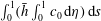$\int _{0}^{1}(\bar{h}\int _{0}^{1}c_{0}\,\text{d}\unicode[STIX]{x1D702})\,\text{d}s$ , is indicated on the side of each individual panel.

Results of integrations of (3.9) for $\unicode[STIX]{x1D70E}=\unicode[STIX]{x1D700}^{2}S=10$ and $\unicode[STIX]{x1D70E}=\unicode[STIX]{x1D700}^{2}S=1$ are shown in figures 6(a) and 6(b), respectively, while figure 6(c) shows results for $1\ll S\ll \unicode[STIX]{x1D700}^{-2}$ , obtained from (3.13), and figure 6(d) shows results for $S=1$ , computed with use of (3.33). With the characteristic value of $\unicode[STIX]{x1D700}$ being of order $\unicode[STIX]{x1D700}\sim 1/50$ and the Schmidt number of drugs typically used in ITDD procedures being of order $S\sim 1000$ , it appears that the conditions investigated in figure 6(b) are directly relevant to drug dispersion in the spinal canal, while the results for $\unicode[STIX]{x1D70E}=\unicode[STIX]{x1D700}^{2}S=10$ , corresponding to Schmidt numbers of order $S\sim 25\,000$ , are representative of transport of radioactive or fluorescence tracers, used in clinical studies. On the other hand, the results for $S=1$ , corresponding to mixing of two gases, are included to illustrate effects of Taylor dispersion and the intermediate case $1\ll S\ll \unicode[STIX]{x1D700}^{-2}$ is included to test the predictive capability of the simplified transport equation (3.13).

For all of the computations shown in figure 6 the initial concentration is given by the Gaussian distribution $c_{i}=\exp [-16^{2}(x-0.75)^{2}]$ . The integration of (3.9) employs the boundary conditions $\unicode[STIX]{x2202}c_{0}/\unicode[STIX]{x2202}\unicode[STIX]{x1D702}=0$ at $\unicode[STIX]{x1D702}=0,1$ , corresponding to impermeable bounding surfaces. Additionally, a boundary condition must be specified for $c_{0}$ at the open boundary $x=0$ . Since convection is the only axial transport mechanism in (3.9), the appropriate condition is determined by the sign of $u_{L}$ at $x=0$ , indicated by blue (upward) and red (downward) colours in the upper left circular plot of figure 2. In regions of upward flow (negative values of $u_{L}$ ) the concentration is given by that within the canal at earlier times, whereas in regions of downward flow (positive values of $u_{L}$ ) the concentration is that found outside the canal, assumed to be $c_{0}=0$ in our integrations. The same boundary conditions are used at the canal entrance $x=0$ when integrating (3.13). On the other hand, the presence of Taylor dispersion in (3.33), involving second-order spatial derivatives, necessitates introduction of suitable modified boundary conditions at the entrance $x=0$ , but not at the closed end $x=1$ , because there the diffusion rate vanishes as a result of the zero values of $D_{xx}$ , $D_{xs}$ and $D_{sx}$ , which are apparent in the plots of figure 4. As discussed by Hydon & Pedley (Reference Hydon and Pedley1993) in connection with axial dispersion in a channel with oscillating walls, the determination of the entry conditions requires in principle consideration of the flow outside the canal, which would be dependent upon the specific geometry found there. To avoid this complicating aspect of the problem, in the integrations reported in figure 6(d) we chose a simplified computational strategy, in which the axial diffusive transport across the boundary at $x=0$ is eliminated, and in which the axial convective transport is treated as described before, i.e. in regions of inflow the concentration is set to zero, whereas in regions of outflow it is determined by its value within the canal at earlier times.

A notable finding of the numerical integrations in figure 6 is the striking qualitative agreement of the different transport patterns, that being a result of the dominant effect of convection driven by the Lagrangian motion, with the axial velocity $u_{L}$ largely determining the evolution of the solute in all cases. As expected from the distributions of $u_{L}$ shown in figure 3, regardless of the Schmidt number the solute is transported rapidly towards the canal entrance along the preferential path $s=0$ (or $s=1$ ), corresponding to the narrow part of the canal where we find large negative values of  $u_{L}$ .

The extent of the effects of Taylor dispersion can be assessed by comparing the snapshots in figure 6(d), corresponding to $S=1$ , with the dispersion-free results shown in figure 6(c) for the same rescaled times. As can be seen, even for this large diffusivity case $S=1$ , the differences between both sets of computations are not significant, and are mainly observed in the solute distribution in the low velocity region near the closed end, where the effect of Taylor dispersion tends to spread the solute concentration. Additional results of integrations of (3.33) for $S=50$ , not shown in figure 6, gave solute distributions that are virtually indistinguishable from those shown in figure 6(c). These findings, consistent with the quantitative results in figure 5, indicate that Taylor dispersion, which is known to play a central role in axial dispersion in axisymmetric or planar configurations, contributes negligibly to the transport of drugs delivered intrathecally in the spinal canal.

As previously discussed, for $S\ll \unicode[STIX]{x1D700}^{-2}$ the solute concentration is uniform across the width of the canal in the first approximation, while in the opposite case $S\gg \unicode[STIX]{x1D700}^{-2}$ molecular diffusion is entirely negligible, so that each fluid particle conserves its initial concentration. An intermediate behaviour is found in the distinguished limit $S\sim \unicode[STIX]{x1D700}^{-2}$ , the case considered in figure 6(a,b), where transverse molecular diffusion is significant, although it is not able to uniformize completely the solute concentration. As a result, the solute located initially near the bounding surfaces $\unicode[STIX]{x1D702}=0$ and $\unicode[STIX]{x1D702}=1$ , where the velocity is small, tends to remain at the initial location, an effect that is clearly visible in the computations for $\unicode[STIX]{x1D70E}=\unicode[STIX]{x1D700}^{2}S=10$ in figure 6(a). Away from the walls the solute is convected by the flow, so that the resulting transport pattern in figure 6(a,b) is similar to figure 6(c).

To provide a more direct quantitative assessment of the effects of the Schmidt number on solute dispersion, the value of the solute flux $\unicode[STIX]{x1D719}_{c}$ was computed at three different sections $x=(0,0.25,0.5)$ for the solute evolutions of figure 6 and also for additional computations with $S=50$ based on (3.33). The value of $\unicode[STIX]{x1D719}_{c}(x,\unicode[STIX]{x1D70F})$ is evaluated from (3.11) in the integrations for $\unicode[STIX]{x1D70E}=\unicode[STIX]{x1D700}^{2}S=10$ and $\unicode[STIX]{x1D70E}=\unicode[STIX]{x1D700}^{2}S=1$ and from (3.36) in the integrations for $S=1$ and $S=50$ , with the simpler expression

(4.2) $$\begin{eqnarray}\unicode[STIX]{x1D719}_{c}=\ell \int _{0}^{1}\left(\int _{0}^{1}u_{L}\,\text{d}\unicode[STIX]{x1D702}\right)c_{0}\bar{h}\,\text{d}s\end{eqnarray}$$

applying in the intermediate limit $1\ll S\ll \unicode[STIX]{x1D700}^{-2}$ . The results are represented in figure 7.

Since the solute migrates towards the canal entrance, the corresponding values of $\unicode[STIX]{x1D719}_{c}$ are negative. The curves at different sections display the expected delay associated with the distance from the injection location ( $x=0.75$ ). The differences in the temporal variation of the solute flux between the extreme values of the Schmidt number $\unicode[STIX]{x1D700}^{2}S=10$ and $S=1$ can be attributed to their distinct convective transport. For the least diffusive case ( $\unicode[STIX]{x1D700}^{2}S=10$ ) the concentration of each fluid particle remains almost constant, so that particles located initially near the centre of the canal $\unicode[STIX]{x1D702}=0.5$ , where the velocity is higher, tend to move faster, whereas those near the bounding surfaces $\unicode[STIX]{x1D702}=(0,1)$ move more slowly. By way of contrast, for $S=1$ the concentration, uniform in $\unicode[STIX]{x1D702}$ , is convected with the width-averaged velocity, smaller than the peak velocity found near the centre. As a result, for $\unicode[STIX]{x1D700}^{2}S=10$ the flux $\unicode[STIX]{x1D719}_{c}$ increases earlier than that for $S=1$ , because of the rapid motion of the fluid particles near the centre of the canal, but reaches a peak value that is significantly lower, because near-wall fluid particles take a long time to move from the initial location. The differences between the other three curves ( $S=50$ , $1\ll S\ll \unicode[STIX]{x1D700}^{2}$ and $\unicode[STIX]{x1D70E}=\unicode[STIX]{x1D700}^{2}S=1$ ) are much smaller, with associated predictions of solute flux differing typically by approximately 10 %. This quantitative agreement suggests that the simplified transport model (3.13), involving only convection driven by the width-averaged Lagrangian velocities, can provide a sufficiently accurate description for many purposes. Additional computations involving canals with more complicated geometries would be needed to ascertain the level of accuracy to be expected in predictive studies for ITDD applications.