


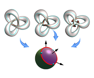

1. Introduction
The dynamics of an ideal flow is governed by the three-dimensional (3-D) incompressible Euler equation. We apply the spherical Clebsch mapping (Kuznetsov & Mikhailov Reference Kuznetsov and Mikhailov1980) to develop the spin Euler equation based on the spin vector – a unit vector encoding vortex lines – instead of the velocity. Given a smooth initial spin vector with proper boundary conditions, the spin Euler equation is equivalent to the classical Euler equation. The spin Euler equation facilitates a viable Lagrangian study of fluid dynamics, as the isosurface of a spin-vector component is a vortex surface (Yang & Pullin Reference Yang and Pullin2010; Yang, Xiong & Lu Reference Yang, Xiong and Lu2023). On the other hand, a globally smooth spin vector may not exist for a given velocity field with vorticity nulls or unclosed vortex lines. Hence the spin Euler equation admits only a subset of initial conditions of the Euler equation.
The present study employs the spin Euler equation to examine the possibility of a finite-time singularity in ideal flows. One of the outstanding open problems in fluid mechanics is whether smooth initial data can lead to finite-time singularities in the ideal flow. This problem is closely related to the existence and smoothness of solutions to the Navier–Stokes equation (e.g. Fefferman Reference Fefferman2001; Doering Reference Doering2009; Wei Reference Wei2016; Ayala & Protas Reference Ayala and Protas2017).
The regularity of the incompressible Euler equation has been studied extensively. Various criteria for blowup and non-blowup, based on different quantities and techniques, have been reviewed by Chae (Reference Chae2008), Gibbon (Reference Gibbon2008) and Drivas & Elgindi (Reference Drivas and Elgindi2023). Several criteria relate the occurrence of singularity to the growth of the vorticity  $\boldsymbol {\omega }$, which plays a vital role in fluid dynamics. The Beale–Kato–Majda (BKM) criterion establishes a sufficient condition for the regularity in terms of
 $\boldsymbol {\omega }$ (Beale, Kato & Majda Reference Beale, Kato and Majda1984). The geometric criterion of Constantin, Fefferman & Majda (Reference Constantin, Fefferman and Majda1996) relates the regularity of the velocity to the smoothness of the vorticity direction. Moreover, there are some refined analytical criteria for blowup (e.g. Planchon Reference Planchon2003; Zhou & Lei Reference Zhou and Lei2013).
The regularity of the incompressible Euler equations has also been investigated by large-scale numerical simulations. Brachet et al. (Reference Brachet, Meiron, Orszag, Nickel, Morf and Frisch1983, Reference Brachet, Meneguzzi, Vincent, Politano and Sulem1992) and Bustamante & Brachet (Reference Bustamante and Brachet2012) conducted numerical studies of the evolution of the inviscid Taylor–Green flow, and showed a near-exponential growth of the maximum vorticity over time, with regions of the high vorticity predominantly confined within thin, sheet-like structures. The formation of vortex sheets reduces the three-dimensionality, which suppresses the formation of a finite-time singularity (Constantin et al. Reference Constantin, Fefferman and Majda1996; Drivas & Elgindi Reference Drivas and Elgindi2023).
As the regularity of the two-dimensional (2-D) Euler equations was established (Yudovich Reference Yudovich1963; Majda & Bertozzi Reference Majda and Bertozzi2002), subsequent numerical studies focused primarily on the carefully designed initial condition that would enhance the vorticity growth. However, different vorticity growth trends were observed in the numerical simulations with different initial conditions or even the same initial condition.
For the two perturbed anti-parallel vortex tubes, Kerr (Reference Kerr1993, Reference Kerr2005) found  $\| \boldsymbol {\omega } \|_\infty \sim (t_0-t)^{-1}$, which provided strong evidence in favour of blowup, whereas Hou & Li (Reference Hou and Li2007) and Hou (Reference Hou2009) obtained a high-resolution numerical solution that is still regular beyond the presumed blowup time
 $t_0$, and exhibited a maximum vorticity growth slower than double-exponential. The analysis was subsequently revisited in Bustamante & Kerr (Reference Bustamante and Kerr2008), who proposed a hypothesis of vorticity growth
 $\| \boldsymbol {\omega } \|_\infty \sim (t_0-t)^{-\gamma }$, with
 $\gamma >1$, and in Kerr (Reference Kerr2013), who reported a double-exponential growth.
The vorticity growth of  $\| \boldsymbol {\omega } \|_\infty \sim (t_0-t)^{-1}$ was also observed in Grauer, Marliani & Germaschewski (Reference Grauer, Marliani and Germaschewski1998) using a perturbed cylindrical shear flow, and in Orlandi, Pirozzoli & Carnevale (Reference Orlandi, Pirozzoli and Carnevale2012) using the collision of two Lamb dipoles. Agafontsev, Kuznetsov & Mailybaev (Reference Agafontsev, Kuznetsov and Mailybaev2015, Reference Agafontsev, Kuznetsov and Mailybaev2017) reported that the vorticity grows exponentially in time in a shear flow with random perturbations. Moreover, Ricca, Samuels & Barenghi (Reference Ricca, Samuels and Barenghi1999) suggested that the vortex knot is a useful configuration for studying singularity formation, and also pointed out the lack of study on the evolution of vortex knots or links with finite thickness in ideal flows.
Several studies examined the Kida–Pelz flow (Kida Reference Kida1985; Boratav & Pelz Reference Boratav and Pelz1994; Pelz Reference Pelz2001), which is another highly symmetric flow for investigating the formation of potential finite-time singularity. Grafke et al. (Reference Grafke, Homann, Dreher and Grauer2008) compared different numerical methods applied to a Kida–Pelz flow in spectral and real spaces, and found no evidence of blowup at the times predicted by previous studies, which was confirmed by Hou & Li (Reference Hou and Li2008). They also observed that the vorticity increases exponentially along the Lagrangian trajectory.
Furthermore, there are several studies that are not based on the Euler equation for investigating potential finite-time singularities in ideal flows. Campolina & Mailybaev (Reference Campolina and Mailybaev2018) developed a model identical to the Euler equations by imitating the calculus on a 3-D logarithmic lattice. This model for ideal flows elucidates the emergence of singularities as a manifestation of a chaotic attractor in a renormalized dynamical system. Their results implied that the direct numerical simulations (DNS) with the available resolution are inadequate for the analysis of singularity formation for the Euler equation. By employing a level-set representation for the vorticity field, Constantin (Reference Constantin2001a,Reference Constantinb) and Deng, Hou & Yu (Reference Deng, Hou and Yu2005) established global existence theorems for a wide range of initial values, and revealed the geometric structures of plausible blowup scenarios, for the 3-D Euler equations and the 3-D Lagrangian averaged Euler equations.
In the present study, we investigate the Lagrangian dynamics and regularity of the spin Euler equation, and derive a new non-blowup condition for ideal flows. The DNS were conducted for solving the spin Euler equation with the pseudo-spectral method in various inviscid vortical flows. The outline of the present paper is as follows. Section 2 introduces the spin Euler equation and derives the non-blowup condition. Section 3 describes numerical set-ups and methods. Section 4 elucidates Lagrangian dynamics of ideal flows and assesses the non-blowup criterion. Some conclusions are drawn in § 5.
2. Theoretical framework of the spin Euler equation
2.1. Introduction to the spin Euler equation
The 3-D incompressible Euler equation is
 \begin{equation} \partial_t\boldsymbol{u} + \boldsymbol{u}\boldsymbol{\cdot}\boldsymbol{\nabla}\boldsymbol{u} ={-} \boldsymbol{\nabla} p, \end{equation}
with  $\boldsymbol {\nabla }\boldsymbol {\cdot }\boldsymbol {u} = 0$, where
 $\boldsymbol {u}$ is the velocity, and
 $p$ is the pressure.
By applying the spherical Clebsch mapping with a Hamiltonian structure (Kuznetsov & Mikhailov Reference Kuznetsov and Mikhailov1980), (2.1) is transformed into a Lagrangian form
 \begin{equation} \partial_t\boldsymbol{s} + \boldsymbol{u}\boldsymbol{\cdot}\boldsymbol{\nabla}\boldsymbol{s} = \boldsymbol{0}, \end{equation}
where  $\boldsymbol {s}$ is of class
 $C^k$,
 $k\ge 1$. Note that
 $\boldsymbol {u}$ can be obtained from
 $\boldsymbol {s}$, which is discussed further in (3.1). Here, the Hopf fibration (Hopf Reference Hopf1931)
 \begin{equation} \boldsymbol{s} = (a^2+b^2-c^2-d^2, 2(bc-ad), 2(ac+bd)) \end{equation}
with  $|\boldsymbol {s}|=1$ establishes a correspondence between the unit spin vector
 $\boldsymbol {s}\in \mathbb {S}^2$ and a two-component wave function
 $\boldsymbol {\psi }=[\psi _1,\psi _2]^{\mathrm {T}}\in \mathbb {S}^3$ (Chern et al. Reference Chern, Knöppel, Pinkall, Schröder and Weißmann2016; Chern Reference Chern2017), where
 $\psi _1=a+\mathrm {i} b$ and
 $\psi _2=c+\mathrm {i} d$ are complex functions of real-valued potentials
 $a,b,c, d$, and
 $\mathrm {i}$ denotes the imaginary unit. The Clebsch potentials
 $a,b,c,d$ are subject to the constraint
 $a\,\Delta b-b\,\Delta a+c\,\Delta d-d\,\Delta c=0$, which ensures the incompressibility
 $\boldsymbol {\nabla }\boldsymbol {\cdot }\boldsymbol {u}=0$.
Then the velocity and vorticity  $\boldsymbol {\omega }\equiv \boldsymbol {\nabla }\times \boldsymbol {u}$ can be re-expressed by
 $\boldsymbol {u} = a\,\boldsymbol {\nabla } b - b\,\boldsymbol {\nabla } a\, +$
 $c\,\boldsymbol {\nabla } d - d\,\boldsymbol {\nabla } c$ and
 \begin{align} \boldsymbol{\omega} &= \tfrac{1}{4}\varepsilon_{ijk}s_i\,\boldsymbol{\nabla} s_j\times \boldsymbol{\nabla} s_k \nonumber\\ &= \tfrac{1}{2}\left(s_1\,\boldsymbol{\nabla} s_2\times\boldsymbol{\nabla} s_3 + s_2\,\boldsymbol{\nabla} s_3\times\boldsymbol{\nabla} s_1 + s_3\,\boldsymbol{\nabla} s_1\times\boldsymbol{\nabla} s_2 \right), \end{align}
respectively, where  $\varepsilon _{ijk}$ is the Levi–Civita symbol. The derivation of (2.4) is detailed in Appendix A. Note that
 $\boldsymbol {s}$ remains a gauge invariant in the transformation from the velocity to ‘magnetization’ (Chorin Reference Chorin1994).
From the perspective of vortex dynamics, the spin vector encodes vortex lines and surfaces (Chern et al. Reference Chern, Knöppel, Pinkall, Schröder and Weißmann2016; Chern Reference Chern2017; Yang et al. Reference Yang, Xiong and Lu2023). Isosurfaces of one component of  $\boldsymbol {s}$ are a family of vortex surfaces. Correspondingly, intersections of isosurfaces of two components of
 $\boldsymbol {s}$ are a family of vortex lines.
We consider the quaternion form (Gibbon & Holm Reference Gibbon and Holm2007) of the two-component wave function  $\boldsymbol {\psi }=a+\boldsymbol {i}b+\boldsymbol {j}c+\boldsymbol {k}d$, where
 $\{\boldsymbol {i},\boldsymbol {j},\boldsymbol {k}\}$ are the basis vectors of the imaginary part of the quaternion. The velocity and spin vector are then given by
 $\boldsymbol {u}=(\boldsymbol {\nabla }\bar {\boldsymbol {\psi }}\boldsymbol {i\psi } - \bar {\boldsymbol {\psi }}\boldsymbol {i}\,\boldsymbol {\nabla }\boldsymbol {\psi })/2$ and
 $\boldsymbol {s}=\bar {\boldsymbol {\psi }}\boldsymbol {i\psi }$, respectively, where
 $\bar {\boldsymbol {\psi }}$ denotes the quaternion conjugate of
 $\boldsymbol {\psi }$. Then we derive
 \begin{align} \boldsymbol{u}\boldsymbol{\cdot}\boldsymbol{\nabla}\boldsymbol{s} &= \tfrac{1}{2}\left(\boldsymbol{\nabla}\bar{\boldsymbol{\psi}}\boldsymbol{i\psi}\boldsymbol{\cdot} \boldsymbol{\nabla}\bar{\boldsymbol{\psi}}\boldsymbol{i\psi} - |\boldsymbol{\nabla}\boldsymbol{\psi}|^2 + |\boldsymbol{\nabla}\boldsymbol{\psi}|^2 - \bar{\boldsymbol{\psi}}\boldsymbol{i}\,\boldsymbol{\nabla}\boldsymbol{\psi}\boldsymbol{\cdot}\bar{\boldsymbol{\psi}}\boldsymbol{i}\,\boldsymbol{\nabla}\boldsymbol{\psi}\right) \nonumber\\ &= \tfrac{1}{2}\left(\boldsymbol{s}\,\boldsymbol{\nabla}\bar{\boldsymbol{\psi}}\boldsymbol{\cdot}\boldsymbol{i}\,\boldsymbol{\nabla}\boldsymbol{\psi} -\boldsymbol{\nabla}\bar{\boldsymbol{\psi}}\boldsymbol{\cdot}\boldsymbol{i}\,\boldsymbol{\nabla}\boldsymbol{\psi}\boldsymbol{s}\right) = \boldsymbol{s}\times\boldsymbol{m}, \end{align}
where  $\boldsymbol {m} \equiv \boldsymbol {\nabla }\bar {\boldsymbol {\psi }}\boldsymbol {\cdot }\boldsymbol {i}\,\boldsymbol {\nabla }\boldsymbol {\psi }$ is a pure quaternion (i.e. a vector in
 $\mathbb {R}^3$) and can be expanded as
 $\boldsymbol {m}=\boldsymbol {i}m_1+\boldsymbol {j}m_2+\boldsymbol {k}m_3$, with
 \begin{equation} \left.\begin{aligned}
m_1 &= |\boldsymbol{\nabla} a|^2 + |\boldsymbol{\nabla} b|^2
- |\boldsymbol{\nabla} c|^2 - |\boldsymbol{\nabla} d|^2, \\
m_2 &= 2(\boldsymbol{\nabla}
b\boldsymbol{\cdot}\boldsymbol{\nabla} c -
\boldsymbol{\nabla} a\boldsymbol{\cdot}\boldsymbol{\nabla}
d), \\ m_3 &= 2(\boldsymbol{\nabla}
a\boldsymbol{\cdot}\boldsymbol{\nabla} c +
\boldsymbol{\nabla} b\boldsymbol{\cdot}\boldsymbol{\nabla}
d). \end{aligned}\right\}
\end{equation}
Thus we rewrite  $\boldsymbol {u}\boldsymbol {\cdot }\boldsymbol {\nabla }\boldsymbol {s}= \boldsymbol {s}\times \boldsymbol {m}$ with an effective field
 $\boldsymbol {m}=(m_1,m_2,m_3)$.
In general,  $\boldsymbol {m}$ cannot be represented solely in terms of
 $\boldsymbol {s}$, because the Hopf mapping (2.3) is non-invertible. However, given
 $\boldsymbol {s}$ with a boundary condition, we can obtain
 $\boldsymbol {u}$ by calculating
 $\boldsymbol {\omega }$ with (2.4) and applying the generalized Biot–Savart law, and then obtain
 $\boldsymbol {s}\times \boldsymbol {m}$ at any point in
 $\mathbb {R}^3$ by (2.5).
Substituting (2.5) into (2.2), we obtain the spin Euler equation
 \begin{equation} \partial_t\boldsymbol{s} + \boldsymbol{s}\times\boldsymbol{m} = \boldsymbol{0}. \end{equation}
This is equivalent to the original incompressible Euler equation (2.1). In contrast to (2.2), (2.7) characterizes the evolution of  $\boldsymbol {s}$ by its precession about
 $\boldsymbol {m}$ rather than the convection with
 $\boldsymbol {u}$. The spin Euler equation (2.7) can be more suitable to study fluid dynamics from a Lagrangian perspective than its original form (2.1), because the isosurfaces of
 $s_i$,
 $i=1,2,3$, are vortex surfaces consisting of vortex lines (Yang & Pullin Reference Yang and Pullin2010, Reference Yang and Pullin2011; Yang et al. Reference Yang, Xiong and Lu2023). From the Helmholtz vorticity laws, the surfaces are material surfaces for all
 $t\ge 0$ in Euler flows.
Therefore, solving the spin Euler equation (2.7) is similar to a vortex method (Yang et al. Reference Yang, Xiong, Zhang, Feng, Liu and Zhu2021; Nabizadeh et al. Reference Nabizadeh, Wang, Ramamoorthi and Chern2022; Xiong et al. Reference Xiong, Wang, Wang and Zhu2022) for simulating ideal flows. Since the primary variable  $\boldsymbol {s}$ of (2.7) has unit length, the fixed magnitude of
 $\boldsymbol {s}$ can avoid the numerical blowup arising from numerical instabilities.
In particular, the spin Euler equation contains the inherent Lagrangian vortex dynamics via level sets of  $s_i$ (i.e. vortex surfaces). This can facilitate the regularity analysis of the Euler equation, similar to the level set representation of
 $\boldsymbol {\omega }$ (Constantin Reference Constantin2001a,Reference Constantinb; Deng et al. Reference Deng, Hou and Yu2005).
Note that the initial conditions  $\boldsymbol {s}_0$ of (2.7) for simulating ideal flows are a subset of the classical Euler equations, because finding a globally smooth
 $\boldsymbol {s}_0$ for a given vorticity field
 $\boldsymbol {\omega }_0$ remains an open problem. Currently, a useful approximation of
 $\boldsymbol {s}_0$ can be obtained using the numerical optimization (Chern et al. Reference Chern, Knöppel, Pinkall and Schröder2017) and the Poincaré recurrence theorem (Poincaré Reference Poincaré1890).
The spin Euler equation is also equivalent to a special case of the Landau–Lifshitz equation with a specific effective magnetic field  $\boldsymbol {m}$, revealing a possible connection between ideal flow and magnetic crystal. As sketched in figure 1, the spin vector (or magnetization)
 $\boldsymbol {s}$ in (2.3) at each point in space precesses around the effective magnetic field
 $\boldsymbol {m}$ in (2.6). More discussion is provided in Appendix B.
The domain is discretized on a uniform grid. The smallest lattice configuration, consisting of  $2^3$ grid points, is sketched. (a) Schematic of a
 $2^3$ lattice of spin vectors, where the orientation of
 $\boldsymbol {s}$ fully characterizes the ideal flow by (2.4). (b) At each grid point, the spin vector
 $\boldsymbol {s}$ in (2.3) precesses around an ‘effective magnetic field’
 $\boldsymbol {m}$ in (2.6).

2.2. Non-blowup condition of the spin Euler equation
Next, we discuss the regularity of the spin Euler equation. The derivation for the non-blowup condition is outlined below and detailed in Appendix C. First, we estimate the upper bound of  $\| \boldsymbol {\omega } \|_p$ in terms of
 $\| \boldsymbol {\nabla }\boldsymbol {s} \|_{2p}$,
 $p\ge 1$, as
 \begin{equation} \|\boldsymbol{\omega}\|_{p} \le \tfrac{1}{2}\,\|\boldsymbol{\nabla}\boldsymbol{s}\|_{{2p}}^2, \end{equation}
where the  $L^p$-norm is defined in Appendix C. Then we estimate the growth of
 $\| \boldsymbol {\nabla }\boldsymbol {s} \|_{2p}$ as
 \begin{equation} \partial_t\| \boldsymbol{\nabla}\boldsymbol{s} \|_{{2p}}^{2p} \le 2p\,\| \boldsymbol{m} \|_{1}\,\| \Delta\boldsymbol{s} \|_{\infty}^p, \end{equation}
and the upper bound of  $\| \boldsymbol {m} \|_1$ in terms of
 $\| \boldsymbol {\nabla }\boldsymbol {s} \|_2$ and
 $\| \Delta \boldsymbol {s} \|_\infty$ as
 \begin{equation} \| \boldsymbol{m} \|_{1}\le \tfrac{1}{4}\,\| \boldsymbol{\nabla}\boldsymbol{s} \|_{2}^2\left(\sqrt{6} + \sqrt{2}C_\omega\,\| \Delta\boldsymbol{s} \|_{\infty} \right), \end{equation}
where  $C_\omega$ is a positive constant. Finally, substituting (2.9) and (2.10) into (2.8), we obtain a sufficient condition for bounded
 $\| \boldsymbol {\omega } \|_p$ as
 \begin{equation} \int_0^t\| \Delta\boldsymbol{s}(\,\cdot\,,\tau) \|_{\infty}^{p+1}\,{\rm d}\tau < \infty, \quad \forall p\ge 1. \end{equation}
In summary, we obtain a non-blowup condition (2.11) of the spin Euler equation (equivalent to the original Euler equation with well-posed initial conditions), which guarantees a bounded  $\| \boldsymbol {\omega } \|_{p}$. It implies that if the solution loses regularity beyond a certain time, then the Laplacian of the spin vector must grow unboundedly. The transport equation and the estimation of the norm of
 $\Delta \boldsymbol {s}$ are discussed further in Appendix D.
3. Numerical set-up
We conduct the DNS of three ideal flows with different initial conditions in a periodic cube of side  $2{\rm \pi}$ on
 $N^3$ (up to
 $1536^3$) uniform grid points, by solving the spin Euler equation (2.2) with the pseudo-spectral method as
 \begin{equation} \left.\begin{aligned}
&\dfrac{\partial\boldsymbol{s}}{\partial t} =
\mathcal{F}^{{-}1}\left[\dfrac{1}{|\boldsymbol{\kappa}|^2}\,\mathrm{i}\mathcal{F}
\left(\dfrac{1}{4}\,\varepsilon_{ijk}s_i\,\boldsymbol{\nabla}
s_j\times \boldsymbol{\nabla} s_k \right)
\times\boldsymbol{\kappa}
\right]\boldsymbol{\cdot}\boldsymbol{\nabla}\boldsymbol{s},\\[9pt]
&\boldsymbol{s}(\boldsymbol{x},t=0) =
\boldsymbol{s}_0(\boldsymbol{x}). \end{aligned}\right\}
\end{equation}
Here,  $\boldsymbol {u}$ is calculated from
 $\boldsymbol {\omega }$ with (2.4) by the Biot–Savart law in Fourier space (Xiong & Yang Reference Xiong and Yang2020),
 $\boldsymbol {\kappa }$ denotes the wavenumber vector,
 $\boldsymbol {s}_0$ is a smooth initial condition, and
 $\mathcal {F}$ is the Fourier transform operator with its inverse form
 $\mathcal {F}^{-1}$. The high-order Fourier smoothing method (Hou & Li Reference Hou and Li2007; Bustamante & Kerr Reference Bustamante and Kerr2008) is used to suppress the Gibbs phenomenon. The temporal evolution is integrated using an explicit second-order Runge–Kutta scheme with adaptive time steps in physical space. The time step is selected to ensure that the Courant–Friedrichs–Lewy number is smaller than 0.3 for numerical stability and accuracy. In the numerical implementation,
 $\boldsymbol {s}$ is normalized at every time step to ensure
 $|\boldsymbol {s}|=1$.
We consider two types of initial conditions. For the first type, the initial vorticity is concentrated in a thin closed vortex tube, such as the trefoil knot (Yao, Yang & Hussain Reference Yao, Yang and Hussain2021; Zhao & Scalo Reference Zhao and Scalo2021; Zhao et al. Reference Zhao, Yu, Chapelier and Scalo2021) and Hopf link (Aref & Zawadzki Reference Aref and Zawadzki1991; Kivotides & Leonard Reference Kivotides and Leonard2021; Yao et al. Reference Yao, Shen, Yang and Hussain2022). Under the self-induced velocity, such vortex tubes can be gradually stretched, twisted and flattened, and form nearly singular vortical structures.
We use the rational map (Kedia et al. Reference Kedia, Foster, Dennis and Irvine2016; Tao et al. Reference Tao, Ren, Tong and Xiong2021) to construct smooth  $\boldsymbol {s}_0$. A small twist is applied to the vortex tube by setting
 $P=\alpha$ (Tao et al. Reference Tao, Ren, Tong and Xiong2021), and
 $Q=\alpha ^3+\beta ^2$ and
 $Q=\alpha ^2+\beta ^2$ are chosen for the trefoil knot and the Hopf link, respectively. Here,
 $(P,Q)$ are a pair of complex polynomial functions, and
 $(\alpha,\beta )$ is a mapping of the coordinate system from the Euclidean space
 $\mathbb {R}^3$ to the two-component complex space
 $\mathbb {C}^2$. The function pair
 $(P,Q)$ is normalized and subjected to a divergence-free projection, yielding a two-component wave function
 $\boldsymbol {\psi }_0=[\psi _{1,0},\psi _{2,0}]^{\mathrm {T}}$ that matches the initial field. The initial spin vector
 $\boldsymbol {s}_0$ and vorticity
 $\boldsymbol {\omega }_0$ are then obtained from (2.3) and (2.4), respectively. Additionally, we re-scale the time as
 $t^*=t/(L_0^2/\varGamma )$, with the initial mean length
 $L_0=2\sqrt {2}{\rm \pi} ^{3/2}/\| \boldsymbol {\nabla }\boldsymbol {s}(\cdot,0) \|_{2}$ and the circulation
 $\varGamma$. The trefoil knot has
 $L_0=0.749$ and
 $\varGamma =5.05$, and the Hopf link has
 $L_0=0.773$ and
 $\varGamma =5.24$.
The second type is a modified Taylor–Green (MTG) initial condition (Meng & Yang Reference Meng and Yang2023), with
 \begin{equation} \boldsymbol{s}_0=(\cos x\cos y\cos z,\sqrt{1-\cos^2x\cos^2y\cos^2z}\,\cos 2z,\sqrt{1-\cos^2x\cos^2y\cos^2z}\,\sin 2z) \end{equation}
and
 \begin{equation} \boldsymbol{\omega}_0=(\cos x\sin y\cos z,-\sin x\cos y\cos z,0). \end{equation}
Note that  $\boldsymbol {s}_0$ for this MTG initial condition is different from
 $\boldsymbol {s}_0$ for the standard Taylor–Green initial condition (Taylor & Green Reference Taylor and Green1937; Brachet et al. Reference Brachet, Meiron, Orszag, Nickel, Morf and Frisch1983, Reference Brachet, Meneguzzi, Vincent, Politano and Sulem1992; Bustamante & Brachet Reference Bustamante and Brachet2012); the former in (3.2) has a negligible singularity, and the latter has a weak singularity (Meng & Yang Reference Meng and Yang2023). This highly symmetric MTG flow would not exhibit a finite-time singularity, and this non-blowup case is used to validate the criterion in (2.11). The re-scaling time is
 $t^*=t$. The parameters for all cases are listed in table 1.
DNS cases and parameters.

To evaluate the numerical resolution, we define  $\mathcal {R}(t^*)\equiv 1/(h\,\| \boldsymbol {\nabla }\boldsymbol {s}(\cdot,t^*) \|_{\infty })$, the ratio of the minimum resolved scale to the grid spacing
 $h$. A finer resolution has a larger
 $\mathcal {R}$. The evolution of
 $\mathcal {R}$ for the three initial conditions is shown in figures 2(a)–2(c). Our numerical tests suggest that
 $\mathcal {R}\ge 2$ can be the criterion for well resolving the smallest scale of (3.1). The largest numbers of grid points in the simulation are
 $N^3=1536^3$ for the trefoil knot and the Hopf link, and
 $N^3=1024^3$ for the MTG flow. Based on the criterion, the largest time
 $T_\mathcal {R} \equiv t^*|_{\mathcal {R}=2}$ of the simulation with the satisfactory resolution is given in table 1 for each case.
Evolution of (a–c)  $\mathcal {R}(t^*)\equiv 1/(h\,\| \boldsymbol {\nabla }\boldsymbol {s}(\cdot,t^*) \|_{\infty })$, (d–f)
 $\| \boldsymbol {u} \|_{2}^2/\| \boldsymbol {u}_0 \|_{2}^2$ and (g–i) the helicity, for the (a,d,g) trefoil knot, (b,e,h) Hopf link and (c,f,i) MTG flow, with different grid resolutions. The vertical dashed lines with different colours mark the time with
 $\mathcal {R}=2$ for each resolution. The simulations are well-resolved on the left of the dashed lines.

Additionally, the resolution can be assessed by the conservation of the total energy  $\| \boldsymbol {u} \|_{2}^2$ and the helicity
 $\mathcal {H}=\int _{\mathcal {D}}\boldsymbol {u}\boldsymbol {\cdot }\boldsymbol {\omega }\,{\rm d} V$ (Moreau Reference Moreau1961; Moffatt Reference Moffatt1969; Meng, Shen & Yang Reference Meng, Shen and Yang2023), which are two invariants of the Euler equations. The energy loss is less than 1‰ for
 $\mathcal {R}\ge 2$ in figures 2(d)–2(f), and the helicity is also well conserved in figures 2(g)–2(i).
4. Validation of non-blowup conditions for the spin Euler equation
4.1. Evolution of vortex surfaces
The DNS of the spin Euler equation (2.7) are carried out to investigate Lagrangian dynamics of ideal flows listed in table 1, and to validate the non-blowup criterion (2.11). To illustrate the Lagrangian vortex dynamics, figure 3 shows the top view of the isosurface of  $s_1=0.5$ (i.e. vortex surface) for the trefoil knot at
 $t^*=0$, 0.9 and 1.8. Note that isosurfaces of
 $s_2$ and
 $s_3$ can show similar structures (Tao et al. Reference Tao, Ren, Tong and Xiong2021), and the isosurfaces of
 $|\boldsymbol {\omega }|$ (not shown) fail to capture the complete vortex tube as visualized by
 $s_1$ (as discussed in Xiong & Yang Reference Xiong and Yang2019; Shen et al. Reference Shen, Yao, Hussain and Yang2023).
(a–c) Evolution of the isosurface of  $s_1=0.5$ (vortex surfaces) colour-coded by
 $|\boldsymbol {\omega }|$ for the trefoil knot at
 $t^*=0$, 0.9 and 1.8 in the top view. Some vortex lines (cyan) are integrated and plotted on the isosurfaces. (d) The vortex surface for
 $s_1=0.5$, the region enclosed by this vortex surface, and the three cyan vortex lines are mapped to the red circle, the purple spherical cap within the red circle, and the three cyan points on the Bloch sphere
 $\mathbb {S}^2$, respectively.

Near the three crossings of the initial vortex knot, adjacent parts of the vortex tube are nearly orthogonal. Driven by the self-induced velocity with the Biot–Savart law, the vortex tube and vortex lines are stretched and twisted. The adjacent parts of the vortex knot approach each other, and they are progressively flattened and rolled up, instead of undergoing the vortex reconnection in viscous flows (Yao & Hussain Reference Yao and Hussain2022). The regions with large vorticity magnitude  $|\boldsymbol {\omega }|$ are rapidly stretched into spiral sheets with strong twist.
In figure 3, the evolving vortex surfaces and lines preserve their initial mapping to the red circle and cyan points on  $\mathbb {S}^2$, respectively, due to the Lagrangian nature of the spin Euler equation. Namely, the vortex topology is preserved in ideal flows. In addition, figure 4 shows the top view of the isosurface of
 $s_1=0.5$ for the Hopf link at
 $t^*=0$, 0.88 and 2.19. The structural evolution is similar to that of the trefoil knot.
Evolution of the isosurface of  $s_1=0.5$ (vortex surface) colour-coded by
 $|\boldsymbol {\omega }|$ for the Hopf link at
 $t^*=0$, 0.88 and 2.19 in the top view. Some vortex lines (cyan) are integrated and plotted on the isosurfaces.

Figure 5 plots the contour of  $|\boldsymbol {\omega }|$ on the
 $x$–
 $y$ plane at
 $z=2.55$, and on the
 $y$–
 $z$ plane at
 $x=3.24$ for the trefoil knot, along with the contour lines of
 $s_1$. These planes intersect the point with the largest
 $|\boldsymbol {\omega }|$, so their contours show the most intense swirling motion. In figure 5(b), ‘vorticity pancakes’ (Brachet et al. Reference Brachet, Meneguzzi, Vincent, Politano and Sulem1992) form in the regions of large
 $|\boldsymbol {\omega }|$ among highly stretched and curved vortex surfaces. These structures appear when the vortex surfaces approach each other and undergo strong deformation. The formation of the high-vorticity region within sheet-like structures was observed in the collapse of vortex pairs (e.g. Pumir & Siggia Reference Pumir and Siggia1990; Kerr Reference Kerr1993) and Taylor–Green and Kida–Pelz flows (Yang & Pullin Reference Yang and Pullin2010). Furthermore, we observe the energy spectra with the
 $k^{-3}$ scaling (not shown) in the evolution of the trefoil knot and Hopf link, consistent with the result for the collision of two Lamb dipoles in Orlandi et al. (Reference Orlandi, Pirozzoli and Carnevale2012).
Contour of the vorticity magnitude and contour lines (white) of  $s_1$ for the trefoil knot on (a) the
 $x$–
 $y$ plane at
 $z=2.55$, and (b) the
 $y$–
 $z$ plane at
 $x=3.24$, at
 $t^*=1.8$. The planes intersecting the point with the largest
 $|\boldsymbol {\omega }|$ contain the most intense swirling motion in the flow.

In the highly symmetric MTG flow, a finite-time singularity may not occur according to the theoretical analysis (Constantin et al. Reference Constantin, Fefferman and Majda1996). Figure 6 plots the evolution of the isosurfaces of  $s_1=0.8$ (red) and
 $s_1=-0.8$ (blue) for the MTG flow. A pair of vortex blobs are compressed and flattened into pancakes. Since the vortex surface is compressed in a quasi-2-D configuration, preserving the smoothness
 $\boldsymbol {\nabla }(\boldsymbol {\omega }/|\boldsymbol {\omega }|)$ of the vorticity direction (Constantin et al. Reference Constantin, Fefferman and Majda1996), the MTG flow does not exhibit a finite-time singularity, even though the vorticity grows rapidly (Brachet et al. Reference Brachet, Meneguzzi, Vincent, Politano and Sulem1992).
Evolution of the isosurfaces of  $s_1=0.8$ (red) and
 $s_1=-0.8$ (blue) in the MTG flow: (a)
 $t^{*}=0$, (b)
 $t^{*}=2$, (c)
 $t^{*}=4$.

The comparison of the two types of ideal flows implies that the Euler equation cannot form a singularity in a 2-D process. Constantin et al. (Reference Constantin, Fefferman and Majda1996) proved that if  $\boldsymbol {u}$ remains uniformly bounded and
 $\boldsymbol {\omega }/|\boldsymbol {\omega }|$ stays
 $C^1$, then no singularity can occur. In other words, the vorticity must change its direction very rapidly to form a potential singularity. Note that if a singularity occurs at a vorticity null for all
 $t^*< t_b^*$ (e.g. Elgindi Reference Elgindi2021), then the vorticity direction becomes discontinuous at the time of singularity. The MTG flow vortex lines near the vorticity nulls maintain a quasi-2-D smooth shape, which contradicts the necessary blowup conditions. Hence the MTG flow does not exhibit finite-time singularities. By contrast, the trefoil knot and Hopf link have large vortex-line curvature in figures 3(c) and 4(c), with a rapid change in the vorticity direction.
4.2. Assessment of the non-blowup criterion
We apply (2.11) to the three ideal flows to test the non-blowup criterion based on the spin Euler equation, and compare our criterion to the BKM criterion (Beale et al. Reference Beale, Kato and Majda1984) by examining growth rates of the maximum vorticity and Laplacian spin vector. Before  $t^* = T_\mathcal {R}$,
 $\| \boldsymbol {\omega } \|_{\infty }$ increases by a factor of approximately 16 for the trefoil knot and the Hopf link in figure 7. Both
 $\| \boldsymbol {\omega } \|_{\infty }$ and
 $\| \Delta \boldsymbol {s} \|_{\infty }$ exhibit the nearly double-exponential growth for the trefoil knot and Hopf link. The double-exponential growth of
 $\| \boldsymbol {\omega } \|_{\infty }$ is consistent with the results in Hou & Li (Reference Hou and Li2007) and Kerr (Reference Kerr2013). As the number of grid points increases (up to
 $1536^3$), the growth rate of
 $\| \Delta \boldsymbol {s} \|_{\infty }$ appears to remain constant for the trefoil knot and Hopf link.
Evolution of (a–c) the maximum vorticity and (d–f) the maximum Laplacian spin vector, for (a,d) the trefoil knot, (b,e) the Hopf link and (c,f) MTG flow, with different grid resolutions, respectively. Note that we plot  $\ln \ln (50\| \boldsymbol {\omega } \|_{\infty })$ for the MTG flow, where the factor 50 is used to avoid complex values of the logarithm. The vertical dashed lines with different colours mark the time with
 $\mathcal {R}=2$ for each resolution. The simulations are well-resolved on the left of the dashed lines (shaded in corresponding colours).

The present criterion has some advantages that  $\ln \ln \| \Delta \boldsymbol {s} \|_{\infty }$ grows more slowly than
 $\ln \ln \| \boldsymbol {\omega } \|_{\infty }$ (4–6 times slower), and exhibits better convergence with the mesh resolution. Therefore,
 $\Delta \boldsymbol {s}$ appears to be resolved more easily than
 $\boldsymbol {\omega }$ with the same numerical accuracy. Moreover, the duration of the linear stage for
 $\ln \ln \| \Delta \boldsymbol {s} \|_\infty$ exceeds that for
 $\ln \ln \| \boldsymbol {\omega } \|_\infty$ more than five-fold.
The highly symmetric MTG flow shows no evidence of a finite-time singularity. The profile of  $\ln \ln \| \Delta \boldsymbol {s} \|_\infty$ in figure 7(f) clearly bends downwards before
 $t^* = T_\mathcal {R}$ with
 $N^3=1024^3$. The growth rate of
 $\| \Delta \boldsymbol {s} \|_\infty$ is weaker than double-exponential, whereas the growth of
 $\| \boldsymbol {\omega } \|_\infty$ remains double-exponential in figure 7(c) when
 $t^*< T_{\mathcal {R}}$. Therefore, the criterion based on
 $\Delta \boldsymbol {s}$ can effectively identify the flows that are unlikely to develop a finite-time singularity.
Assuming that the double-exponential growth is bounded in a finite time  $t$, the time integral of
 $\| \Delta \boldsymbol {s} \|_\infty ^{p+1}$ becomes
 \begin{equation} \int_0^t\| \Delta \boldsymbol{s}(\,\cdot\,,\tau) \|_{\infty}^{p+1}\,{\rm d}\tau \le \frac{(\mathrm{e}^{c_1t}-1)\exp[(p+1)\,\mathrm{e}^{c_1t+c_2}]}{c_1\mathrm{e}^{c_1t}}, \end{equation}
with constants  $c_1$ and
 $c_2$. According to the non-blowup condition (2.11), the Euler equation can avoid singularity formation in finite time for the double-exponential growth of
 $\| \Delta \boldsymbol {s} \|_\infty$.
4.3. Difference of non-blowup criteria
We highlight the major difference between (2.11) and the BKM criterion, and explain why  $\| \Delta \boldsymbol {s} \|_{\infty }$ grows more slowly than
 $\| \boldsymbol {\omega } \|_{\infty }$. Figure 8 plots the trajectories of
 $\arg \max |\boldsymbol {\omega }|$ and
 $\arg \max |\Delta \boldsymbol {s}|$, colour-coded by
 $t^*$, and their projections on the
 $x$–
 $y$ plane for the trefoil knot and Hopf link. The trajectories of
 $\arg \max |\boldsymbol {\omega }|$ and
 $\arg \max |\Delta \boldsymbol {s}|$ starting from the same locations do not collapse, implying that the present criterion is distinct from the BKM criterion.
Three groups of trajectories of the maximum points of  $|\boldsymbol {\omega }|$ (from blue to green) and
 $|\Delta \boldsymbol {s}|$ (from red to yellow) during
 $t^*\in [0,2.2]$ for (a) the trefoil knot and (b) the Hopf link, along with their projections on the
 $x$–
 $y$ plane (shaded in grey). The two trajectories of maximum
 $|\boldsymbol {\omega }|$ and
 $|\Delta \boldsymbol {s}|$ in each group start at the same location.

The continuous trajectory of  $\arg \max |\Delta \boldsymbol {s}|$ is more tractable than the discontinuous one of
 $\arg \max |\boldsymbol {\omega }|$ in figure 8. Figure 9 illustrates the
 $z$-coordinates of the maximum
 $|\boldsymbol {\omega }|$ and
 $|\Delta \boldsymbol {s}|$, the Lagrangian trajectory of particles that locate at the position of the maximum values at
 $t^*=0$, and the evolution of the centroid positions
 $z_c = \int _{s_1\ge 0}z\,{\rm d}V /\int _{s_1\ge 0}\,{\rm d}V$ of the trefoil knot and Hopf link. We find that
 $\arg \max |\Delta \boldsymbol {s}|$ remains continuous over time and moves at a constant speed in the
 $z$-direction in both flows, which is close to the Lagrangian velocity of the particle at the location of
 $\arg \max |\Delta \boldsymbol {s}|$ (or
 $\arg \max |\boldsymbol {\omega }|$) at
 $t^*=0$. This implies that the maximum
 $|\Delta \boldsymbol {s}|$ could have some Lagrangian nature.
Evolution of the  $z$-direction coordinates of the maximum points of
 $|\boldsymbol {\omega }|$ and
 $|\Delta \boldsymbol {s}|$, the Lagrangian tracing particle located at the maximum point at
 $t^*=0$, and the centroid position for (a) the trefoil knot and (b) the Hopf link.

By contrast,  $\arg \max |\boldsymbol {\omega }|$ exhibits a sharp jump at
 $t^*=1.26$ for the trefoil knot and
 $t^*=1.98$ for the Hopf link. The speed of
 $\arg \max |\boldsymbol {\omega }|$ in the
 $z$-direction is close to that of the centroid of the vortex at early times. During the growth of
 $|\boldsymbol {\omega }|$, the locus of the peak vorticity exhibits a notable displacement, converging to
 $\arg \max |\Delta \boldsymbol {s}|$ (marked in a dashed box in figure 9).
We examine the correlation and distribution of the values of  $|\Delta \boldsymbol {s}|$ and
 $|\boldsymbol {\omega }|$, normalized by their respective maxima, for the trefoil knot at
 $t^*=1.8$ and the Hopf link at
 $t^*=2.19$. The scatter plots in figure 10 show a low positive correlation between
 $|\Delta \boldsymbol {s}|/\| \Delta \boldsymbol {s} \|_{\infty }$ and
 $|\boldsymbol {\omega }|/\| \boldsymbol {\omega } \|_{\infty }$, with correlation coefficients
 $\rho =0.675$ for the trefoil knot, and
 $\rho =0.627$ for the Hopf link. Therefore, the criterion based on
 $\Delta \boldsymbol {s}$ in (2.11) has a notable statistical difference from that based on
 $\boldsymbol {\omega }$.
Scatter plots of  $|\Delta \boldsymbol {s}|$ and
 $|\boldsymbol {\omega }|$ normalized with their maximum values for (a) the trefoil knot at
 $t^*=1.8$, and (b) the Hopf link at
 $t^*=2.19$, along with the correlation coefficients
 $\rho$ and linear fits (dashed lines) of data points. The scattered points are coloured from purple to red by the density of data points.

The probability density functions (p.d.f.s) of the normalized values of  $|\Delta \boldsymbol {s}|$ and
 $|\boldsymbol {\omega }|$ for the trefoil knot at
 $t^*=1.8$ and the Hopf link at
 $t^*=2.19$ are shown in figure 11. For both configurations, the p.d.f. profiles of
 $|\Delta \boldsymbol {s}|/\| \Delta \boldsymbol {s} \|_{\infty }$ are smoother than those of
 $|\boldsymbol {\omega }|/\| \boldsymbol {\omega } \|_{\infty }$, and they obey a Pareto distribution (Arnold Reference Arnold2015) with the
 $-2$ power law except for very large values, indicating that the extreme values at a few locations can dominate norms of
 $\Delta \boldsymbol {s}$ and
 $\boldsymbol {\omega }$.
P.d.f.s of normalized  $|\Delta \boldsymbol {s}|$ and
 $|\boldsymbol {\omega }|$ for (a) the trefoil knot at
 $t^*=1.8$, and (b) the Hopf link at
 $t^*=2.19$.

5. Conclusions
We develop a new framework for describing ideal flows using the spin Euler equation (2.7). The spin Euler equation can be considered as a special Landau–Lifshitz equation with an effective magnetic field  $\boldsymbol {m}$ in (2.6), implying a possible connection between the ideal flow and magnetic material.
Compared to the classical Euler equation, the spin Euler equation provides a feasible approach to study Lagrangian fluid dynamics, because the isosurfaces of a spin-vector component are vortex surfaces and material surfaces for all  $t\ge 0$. In particular, we derive a non-blowup condition (2.11) for the spin Euler equation – if the solution becomes singular at some finite time, then
 $|\Delta \boldsymbol {s}|$ must become unbounded. Moreover, the ideal flow dynamics is formulated as a Hamiltonian simulation of a quantum mechanical system using the spin Euler equation, which can inspire the development of relevant quantum algorithms (Meng & Yang Reference Meng and Yang2023).
On the other hand, the spin Euler equation does not seem to admit arbitrary velocity fields as initial conditions. The theoretical construction of a globally smooth  $\boldsymbol {s}_0$ for a given velocity field remains an open problem, and it can be approximated only numerically at present.
We conduct the DNS of three ideal flows of the trefoil knot, Hopf link and MTG by solving (3.1) using the pseudo-spectral method, and compare the BKM criterion with the present one. The evolution of the vortex surface (isosurface of  $s_1$) illustrates that the regions with large
 $|\boldsymbol {\omega }|$ are rapidly stretched into spiral sheets for the trefoil knot and Hopf link.
For the trefoil knot and Hopf link, the double-exponential growth of  $\| \Delta \boldsymbol {s} \|_{\infty }$ is more pronounced than that of
 $\| \boldsymbol {\omega } \|_{\infty }$, and
 $\ln \ln \| \Delta \boldsymbol {s} \|_{\infty }$ grows at a rate 4–6 times slower than
 $\ln \ln \| \boldsymbol {\omega } \|_{\infty }$. The duration of the double-exponential growth stage for
 $\| \Delta \boldsymbol {s} \|_\infty$ exceeds that for
 $\| \boldsymbol {\omega } \|_\infty$ by more than five times. According to the non-blowup condition (2.11), the Euler equation can avoid the singularity formation at finite time if the growth rate of
 $\| \Delta \boldsymbol {s} \|_\infty$ is lower than double-exponential at late times.
The highly symmetric MTG flow can avoid finite-time singularities due to the formation of quasi-2-D vortex surfaces from theoretical analysis (Constantin et al. Reference Constantin, Fefferman and Majda1996). The growth rate of  $\| \Delta \boldsymbol {s} \|_\infty$ is lower than double-exponential at late times, whereas the growth rate of
 $\| \boldsymbol {\omega } \|_\infty$ remains double-exponential. Thus the present criterion based on
 $\Delta \boldsymbol {s}$ appears to be more sensitive than the BKM criterion based on
 $\boldsymbol {\omega }$ in detecting the flows that are incapable of producing finite-time singularities.
The present non-blowup criterion based on  $|\Delta \boldsymbol {s}|$ is distinct from the BKM criterion based on
 $|\boldsymbol {\omega }|$. By tracing the maxima of
 $|\Delta \boldsymbol {s}|$ and
 $|\boldsymbol {\omega }|$ for vortex knots and link, we find that the trajectory for
 $|\Delta \boldsymbol {s}|$ is continuous and consistent with the tracer particle, benefited from the Lagrangian nature of the spin Euler equation. In contrast, the trajectory for
 $|\boldsymbol {\omega }|$ with a large jump deviates from the Lagrangian trajectory. Furthermore,
 $|\Delta \boldsymbol {s}|$ and
 $|\boldsymbol {\omega }|$ have only a low positive correlation coefficient.
In future work, the bound estimate of  $|\Delta \boldsymbol {s}|$ requires further refinement, and the duration in the simulation can be prolonged with more computational resources for examining longer growth behaviour of
 $\| \Delta \boldsymbol {s} \|_\infty$. Furthermore, the spin Euler equation can be recast as a nonlinear Schrödinger equation that is useful in quantum computing of fluid dynamics (Meng & Yang Reference Meng and Yang2023).
Acknowledgements
The authors thank S. Xiong for helpful discussion. Numerical simulations were carried out on the TH-2A supercomputer in Guangzhou, China.
Funding
This work has been supported by the National Natural Science Foundation of China (grant nos 11925201 and 11988102), the National Key R&D Program of China (grant no. 2020YFE0204200), and the Xplorer Prize.
Declaration of interests
The authors report no conflict of interest.
Author contributions
Y.Y. and Z.M. designed the research. Z.M. performed the research. Y.Y. and Z.M. discussed the results and wrote the manuscript. Both authors have given approval for the manuscript.
Appendix A. Spherical Clebsch representation of the vorticity
Chern (Reference Chern2017) applied exterior calculus and quaternion formulation to derive the spherical Clebsch representation of  $\boldsymbol {\omega }$ in (2.4). Here, we re-express this derivation using regular calculus. Note that equivalent forms of (2.4) appeared in Faddeev (Reference Faddeev1976) and Kuznetsov & Mikhailov (Reference Kuznetsov and Mikhailov1980) without derivation.
First, we express the vorticity using Clebsch potentials by taking the curl of the velocity as
 \begin{equation} \boldsymbol{\omega} = \boldsymbol{\nabla}\times(a\,\boldsymbol{\nabla} b - b\,\boldsymbol{\nabla} a + c\,\boldsymbol{\nabla} d - d\,\boldsymbol{\nabla} c) = 2(\boldsymbol{\nabla} a\times\boldsymbol{\nabla} b + \boldsymbol{\nabla} c\times\boldsymbol{\nabla} d). \end{equation}
Then we take gradient of the three components of the spin vector as
 \begin{equation} \left.\begin{aligned}
\boldsymbol{\nabla} s_1 &= 2(a\,\boldsymbol{\nabla} a +
b\,\boldsymbol{\nabla} b - c\,\boldsymbol{\nabla} c -
d\,\boldsymbol{\nabla} d), \\ \boldsymbol{\nabla} s_2 &=
2(b\,\boldsymbol{\nabla} c + c\,\boldsymbol{\nabla} b -
a\,\boldsymbol{\nabla} d - d\,\boldsymbol{\nabla} a), \\
\boldsymbol{\nabla} s_3 &= 2(a\,\boldsymbol{\nabla} c +
c\,\boldsymbol{\nabla} a + b\,\boldsymbol{\nabla} d +
d\,\boldsymbol{\nabla} b). \end{aligned}\right\}
\end{equation}
Combining  $\boldsymbol {\nabla } s_1\times \boldsymbol {\nabla } s_2$,
 $\boldsymbol {\nabla } s_2\times \boldsymbol {\nabla } s_3$ and
 $\boldsymbol {\nabla } s_3\times \boldsymbol {\nabla } s_1$, and using the normalization condition
 $a^2+b^2+c^2+d^2=1$, yields
 \begin{align} &s_3\,\boldsymbol{\nabla} s_1\times\boldsymbol{\nabla} s_2 + s_1\,\boldsymbol{\nabla} s_2\times\boldsymbol{\nabla} s_3 + s_2\,\boldsymbol{\nabla} s_3\times\boldsymbol{\nabla} s_1\nonumber\\ &\quad = 4(c^2+d^2)\,\boldsymbol{\nabla} a\times\boldsymbol{\nabla} b + 4(ad-bc)\,\boldsymbol{\nabla} a\times \boldsymbol{\nabla} c - 4(ac+bd)\,\boldsymbol{\nabla} a\times \boldsymbol{\nabla} d \nonumber\\ &\qquad + 4(ac+bd)\,\boldsymbol{\nabla} b\times\boldsymbol{\nabla} c + 4(ad-bc)\,\boldsymbol{\nabla} b\times\boldsymbol{\nabla} d + 4(a^2+b^2)\,\boldsymbol{\nabla} c\times \boldsymbol{\nabla} d. \end{align}
Taking the gradient of the normalization condition yields
 \begin{equation} a\,\boldsymbol{\nabla} a+b\,\boldsymbol{\nabla} b+c\,\boldsymbol{\nabla} c+d\,\boldsymbol{\nabla} d=\boldsymbol{0}. \end{equation}
From (A4) and outer products of two of  $\boldsymbol {\nabla } a$,
 $\boldsymbol {\nabla } b$,
 $\boldsymbol {\nabla } c$ and
 $\boldsymbol {\nabla } d$, we have
 \begin{equation} \left.\begin{aligned}
& b\,\boldsymbol{\nabla} a\times \boldsymbol{\nabla} b +
c\,\boldsymbol{\nabla} a\times\boldsymbol{\nabla} c +
d\,\boldsymbol{\nabla} a\times \boldsymbol{\nabla} d =
\boldsymbol{0}, \\ & a\,\boldsymbol{\nabla} a\times
\boldsymbol{\nabla} b - c\,\boldsymbol{\nabla}
b\times\boldsymbol{\nabla} c - d\,\boldsymbol{\nabla}
b\times \boldsymbol{\nabla} d = \boldsymbol{0}, \\
& a\,\boldsymbol{\nabla} a\times \boldsymbol{\nabla} c +
b\,\boldsymbol{\nabla} b\times \boldsymbol{\nabla} c -
d\,\boldsymbol{\nabla} c\times \boldsymbol{\nabla} d =
\boldsymbol{0}, \\ & a\,\boldsymbol{\nabla} a\times
\boldsymbol{\nabla} d + b\,\boldsymbol{\nabla} b\times
\boldsymbol{\nabla} d + c\,\boldsymbol{\nabla} c\times
\boldsymbol{\nabla} d = \boldsymbol{0}.
\end{aligned}\right\}
\end{equation}
Substituting (A5) into (A3) yields
 \begin{align} &s_3\,\boldsymbol{\nabla} s_1\times\boldsymbol{\nabla} s_2 + s_1\,\boldsymbol{\nabla} s_2\times\boldsymbol{\nabla} s_3 + s_2\,\boldsymbol{\nabla} s_3\times\boldsymbol{\nabla} s_1\nonumber\\ &\quad= 4(a^2+b^2+c^2+d^2)\,\boldsymbol{\nabla} a\times\boldsymbol{\nabla} b + 4(a^2+b^2+c^2+d^2)\,\boldsymbol{\nabla} c\times \boldsymbol{\nabla} d\nonumber\\ &\quad= 4(\boldsymbol{\nabla} a\times \boldsymbol{\nabla} b + \boldsymbol{\nabla} c\times \boldsymbol{\nabla} d). \end{align}
Finally, substituting (A6) into (A1) yields (2.4), i.e.
 \begin{equation} \boldsymbol{\omega} = \tfrac{1}{2}\left(s_1\,\boldsymbol{\nabla} s_2\times\boldsymbol{\nabla} s_3 + s_2\,\boldsymbol{\nabla} s_3\times\boldsymbol{\nabla} s_1 + s_3\,\boldsymbol{\nabla} s_1\times\boldsymbol{\nabla} s_2 \right). \end{equation}
Appendix B. Comparison of the spin Euler system and the isotropic Heisenberg spin system
It is interesting that the spin Euler equation (2.7) can be considered as the Landau–Lifshitz equation
 \begin{equation} \partial_t\boldsymbol{s} + \boldsymbol{s}\times\boldsymbol{H}_{eff} = \boldsymbol{0} \end{equation}
without a damping term (Landau & Lifshitz Reference Landau and Lifshitz1935), which is used to analyse magnetodynamic processes in magnetic materials. Equation (B1) is also recognized as the Heisenberg model with various applications (Lakshmanan & Porsezian Reference Lakshmanan and Porsezian1990; Porsezian & Lakshmanan Reference Porsezian and Lakshmanan1991; Kamppeter et al. Reference Kamppeter, Leonel, Mertens, Gouvêa, Pires and Kovalev2001). The Landau–Lifshitz equation plays an important role in elucidating magnetization dynamics, analogous to the role of the Navier–Stokes equation in fluid dynamics.
The mean spin of electrons, i.e. the magnetization (or spin vector)  $\boldsymbol {s}$ at the macroscopic scale, determines the unit volume magnetic dipole moment in magnetic crystals. A continuous function
 $\boldsymbol {s}(\boldsymbol {x},t)$ describes the macroscopic magnetization dynamics in the limit of vanishing lattice partition size, if the angle between the spin vectors of neighbouring lattice atoms in a crystal is sufficiently small (Heisenberg Reference Heisenberg1928). This resembles the continuum assumption in fluid mechanics, but unlike isotropic fluids, most crystal structures are anisotropic.
In (B1),  $\boldsymbol {H}_{eff}$ is the effective magnetic field, corresponding to (minus) the
 $L^2$-derivative of the magnetic energy of the material with respect to
 $\boldsymbol {s}$. This implies a deep connection between the ideal flow and magnetic material. The spin Euler equation has
 $\boldsymbol {H}_{eff}=\boldsymbol {m}$, where the magnetic energy of a material is replaced by the total kinetic energy of a fluid. Therefore, the ideal flow might be physically interpreted as a specific magnetic material by (2.7).
We then discuss the similarity and difference between the spin Euler system in (2.7) and the isotropic Heisenberg spin system in (B1) with  $\boldsymbol {H}_{eff}=\Delta \boldsymbol {s}$. After some algebra, we find
 \begin{equation} \boldsymbol{m} = \tfrac{1}{2}\,\Delta\boldsymbol{s} + \boldsymbol{m}', \end{equation}
where the term
 \begin{align} \boldsymbol{m}' &= ({-}a\,\Delta a-b\,\Delta b+c\,\Delta c+d\,\Delta d, a\,\Delta d+d\,\Delta a-b\,\Delta c-c\,\Delta b, \nonumber\\ &\quad - a\,\Delta c-c\,\Delta a-b\,\Delta d-d\,\Delta b ) \end{align}
highlights the difference between the spin Euler system and the Heisenberg spin system. Projecting  $\boldsymbol {m}'$ onto
 $\boldsymbol {s}$ yields
 \begin{equation} \boldsymbol{s}\boldsymbol{\cdot}\boldsymbol{m}' ={-}(a\,\Delta a+b\,\Delta b+c\,\Delta c+d\,\Delta d) = |\boldsymbol{\nabla}\boldsymbol{\psi}|^2 \ge 0, \end{equation}
i.e. the angle between  $\boldsymbol {m}'$ and
 $\boldsymbol {s}$ is acute or normal.
As sketched in figure 12, the range of the angle  $\theta \equiv \arccos ((\boldsymbol {s} \boldsymbol {\cdot } \boldsymbol {H}_{eff})/|\boldsymbol {H}_{eff}|)$ between
 $\boldsymbol {s}$ and
 $\boldsymbol {H}_{eff}$ depends on the spin system. The isotropic Heisenberg spin system has
 $\theta \in [{\rm \pi} /2,{\rm \pi} ]$ with
 \begin{equation} \boldsymbol{s} \boldsymbol{\cdot} \boldsymbol{H}_{eff} = \boldsymbol{s} \boldsymbol{\cdot} \Delta \boldsymbol{s} ={-}|\boldsymbol{\nabla} \boldsymbol{s}|^2 \le 0, \end{equation}
whereas the spin Euler system has  $\theta \in [0,{\rm \pi} ]$ with
 \begin{equation} \boldsymbol{s} \boldsymbol{\cdot} \boldsymbol{H}_{eff} = \boldsymbol{s} \boldsymbol{\cdot} \left(\tfrac{1}{2}\,\Delta \boldsymbol{s} + \boldsymbol{m}' \right) = |\boldsymbol{u}|^2 - \tfrac{1}{4}\,|\boldsymbol{\nabla} \boldsymbol{s}|^2. \end{equation}
Assuming that  $\boldsymbol {H}_{eff}$ is directed to the north pole,
 $\boldsymbol {s}$ in the isotropic Heisenberg spin system is confined to the southern hemisphere, whereas there is no such restriction in the spin Euler system due to the additional term
 $\boldsymbol {m}'$. Therefore, the spin Euler system for ideal flows can have greater degrees of freedom and more complex dynamics than the isotropic Heisenberg spin system for magnetic crystals.
Schematic of orientations of the spin vector  $\boldsymbol {s}$ and the effective field
 $\boldsymbol {H}_{eff}$ in (a) the isotropic Heisenberg spin system, and (b) the spin Euler system. The variation of
 $\Delta \boldsymbol {s}$ is restricted to the southern hemisphere (shaded in blue), whereas
 $\boldsymbol {m}'$ is restricted to the northern hemisphere (shaded in red).

Appendix C. Derivation for the non-blowup condition of the spin Euler equation
We provide the detailed derivation for the non-blowup condition (2.11) of the spin Euler equation. By taking the double inner product of  $\boldsymbol {\nabla }\boldsymbol {s}$ and the gradient of (2.7), and multiplying by
 $p\,|\boldsymbol {\nabla }\boldsymbol {s}|^{2(p-1)}$, we obtain
 \begin{equation} \partial_t|\boldsymbol{\nabla}\boldsymbol{s}|^{2p} = 2p\,|\boldsymbol{\nabla}\boldsymbol{s}|^{2(p-1)}\,\boldsymbol{\nabla}\boldsymbol{s}:(\boldsymbol{\nabla}\boldsymbol{m}\times\boldsymbol{s}), \end{equation}
where  $p\ge 1$ is a constant, the double inner product is defined as
 $\boldsymbol{\mathsf{A}}:\boldsymbol{\mathsf{B}}\equiv A_{ij}B_{ij}$ with two second-order tensors
 $\boldsymbol{\mathsf{A}}$ and
 $\boldsymbol{\mathsf{B}}$, and the vector product of the second-order tensor
 $\boldsymbol {\nabla }\boldsymbol {m}$ and the vector
 $\boldsymbol {s}$ is defined as
 $\boldsymbol {\nabla }\boldsymbol {m}\times \boldsymbol {s}\equiv \varepsilon _{ljk}\,\partial _im_js_k\,\boldsymbol {e}_i\boldsymbol {e}_l$ with the basis
 $\{\boldsymbol {e}_1,\boldsymbol {e}_2,\boldsymbol {e}_3\}$. Using the identity
 $\boldsymbol {s}\boldsymbol {\cdot }\Delta \boldsymbol {s}=-|\boldsymbol {\nabla }\boldsymbol {s}|^2$ for the unit vector
 $\boldsymbol {s}$, we have
 \begin{equation} |\boldsymbol{\nabla}\boldsymbol{s}|^2 \le |\Delta\boldsymbol{s}|. \end{equation}
Integrating (C1) over a periodic domain  $\mathcal {D}$ or a domain bounded by solid wall boundaries, and using (C2), yields
 \begin{align} \left|\partial_t\int_{\mathcal{D}}|\boldsymbol{\nabla}\boldsymbol{s}|^{2p} \,{\rm d}V\right| &= 2p\left|\int_{\mathcal{D}}|\boldsymbol{\nabla}\boldsymbol{s}|^{2(p-1)}\,\boldsymbol{\nabla}\boldsymbol{s}:(\boldsymbol{\nabla}\boldsymbol{m}\times\boldsymbol{s})\,{\rm d}V\right| \nonumber\\ &\le 2p\,\| \Delta\boldsymbol{s} \|_{\infty}^{p-1}\left|\int_{\mathcal{D}}\left[\boldsymbol{\nabla} \boldsymbol{\cdot}(\boldsymbol{\nabla}\boldsymbol{s}\boldsymbol{\cdot}(\boldsymbol{m}\times\boldsymbol{s})) + \boldsymbol{m}\boldsymbol{\cdot}(\boldsymbol{\nabla}\boldsymbol{\cdot}(\boldsymbol{\nabla}\boldsymbol{s}\times\boldsymbol{s})) \right]{\rm d}V\right|\nonumber\\ &= 2p\,\| \Delta\boldsymbol{s} \|_{\infty}^{p-1}\left|\displaystyle\unicode{x222F}_{\partial\mathcal{D}}\frac{\partial\boldsymbol{s}}{\partial n}\boldsymbol{\cdot}(\boldsymbol{m}\times\boldsymbol{s})\,{\rm d}S \right.\nonumber\\ &\quad + \left.\int_{\mathcal{D}}[\Delta\boldsymbol{s}\boldsymbol{\cdot}(\boldsymbol{s}\times\boldsymbol{m}) + \boldsymbol{\nabla}\boldsymbol{s}:(\boldsymbol{\nabla}\boldsymbol{s}\times\boldsymbol{m})]\,{\rm d}V\right|\nonumber\\ &= 2p\,\| \Delta\boldsymbol{s} \|_{\infty}^{p-1}\left|\int_{\mathcal{D}}\boldsymbol{m}\boldsymbol{\cdot}(\Delta\boldsymbol{s}\times\boldsymbol{s}) \,{\rm d}V\right|, \end{align}
where the Neumann boundary condition  $\partial \boldsymbol {s}/\partial n|_{\partial \mathcal {D}}=\boldsymbol {0}$ is imposed on the solid wall boundary. Applying the Hölder inequality to (C3) yields
 \begin{equation} \partial_t\| \boldsymbol{\nabla}\boldsymbol{s} \|_{{2p}}^{2p} \le 2p\,\| \boldsymbol{m} \|_{1}\,\| \Delta\boldsymbol{s} \|_{\infty}^p. \end{equation}
Here, the  $L^p$-norm of a function
 $f$ is defined as
 \begin{equation} \|\, f \|_{p} \equiv
\begin{cases}
\left(\displaystyle\int\nolimits_{\mathcal{D}}|\,f|^p\,{\rm
d}V \right)^{1/p}, & 1\le p<\infty, \\[10pt]
\mathrm{esssup}\,|\,f|, & p=\infty. \end{cases}
\end{equation}
We estimate the upper bound of  $\| \boldsymbol {\omega } \|_{p}$ in terms of
 $\| \boldsymbol {\nabla }\boldsymbol {s} \|_{{2p}}$. From (2.4), using
 $|\boldsymbol {s}|=1$ and basic inequalities, we obtain
 \begin{align} |\boldsymbol{\omega}|&\le \tfrac{1}{2}(|\boldsymbol{\nabla} s_1|\,|\boldsymbol{\nabla} s_2| + |\boldsymbol{\nabla} s_2|\,|\boldsymbol{\nabla} s_3| + |\boldsymbol{\nabla} s_3|\,|\boldsymbol{\nabla} s_1|)\nonumber\\ &\le \tfrac{1}{2}\left[\tfrac{1}{2}(|\boldsymbol{\nabla} s_1|^2+|\boldsymbol{\nabla} s_2|^2) + \tfrac{1}{2}(|\boldsymbol{\nabla} s_2|^2+|\boldsymbol{\nabla} s_3|^2) + \tfrac{1}{2}(|\boldsymbol{\nabla} s_3|^2+|\boldsymbol{\nabla} s_1|^2)\right]\nonumber\\ &= \tfrac{1}{2}|\boldsymbol{\nabla}\boldsymbol{s}|^2, \end{align}
so that
 \begin{equation} \|\boldsymbol{\omega}\|_{p} \le \tfrac{1}{2}\,\|\boldsymbol{\nabla}\boldsymbol{s}\|_{{2p}}^2. \end{equation}
Then we estimate the upper bound of  $\| \boldsymbol {m} \|_{1}$ in terms of
 $\| \boldsymbol {\nabla }\boldsymbol {s} \|_{{2}}$ and
 $\| \Delta \boldsymbol {s} \|_{\infty }$. Substituting (C6) into (2.6), we have
 \begin{align} |\boldsymbol{m}|^2&=
|\boldsymbol{\nabla} a|^4 + |\boldsymbol{\nabla} b|^4 +
|\boldsymbol{\nabla} c|^4 + |\boldsymbol{\nabla} d|^4 +
2\,|\boldsymbol{\nabla} a|^2\,|\boldsymbol{\nabla} b|^2 +
2\,|\boldsymbol{\nabla} c|^2\,|\boldsymbol{\nabla}
d|^2\nonumber\\ &\quad - 2\,|\boldsymbol{\nabla}
a|^2\,|\boldsymbol{\nabla} c|^2 - 2\,|\boldsymbol{\nabla}
a|^2\,|\boldsymbol{\nabla} d|^2 - 2\,|\boldsymbol{\nabla}
b|^2\,|\boldsymbol{\nabla} c|^2 - 2\,|\boldsymbol{\nabla}
b|^2\,|\boldsymbol{\nabla} d|^2\nonumber\\ &\quad +
4[(\boldsymbol{\nabla}
b\boldsymbol{\cdot}\boldsymbol{\nabla} c)^2 +
(\boldsymbol{\nabla} a\boldsymbol{\cdot}\boldsymbol{\nabla}
d)^2 - 2(\boldsymbol{\nabla} b\boldsymbol{\cdot}
\boldsymbol{\nabla} c)(\boldsymbol{\nabla}
a\boldsymbol{\cdot}\boldsymbol{\nabla} d)]\nonumber\\
&\quad + 4[(\boldsymbol{\nabla}
a\boldsymbol{\cdot}\boldsymbol{\nabla} c)^2 +
(\boldsymbol{\nabla} b\boldsymbol{\cdot}\boldsymbol{\nabla}
d)^2 + 2(\boldsymbol{\nabla}
a\boldsymbol{\cdot}\boldsymbol{\nabla}
c)(\boldsymbol{\nabla}
b\boldsymbol{\cdot}\boldsymbol{\nabla} d)]\nonumber\\ &\le
(|\boldsymbol{\nabla} a|^2 + |\boldsymbol{\nabla} b|^2 +
|\boldsymbol{\nabla} c|^2 + |\boldsymbol{\nabla} d|^2)^2
\nonumber\\ &\quad + 8[(\boldsymbol{\nabla}
a\boldsymbol{\cdot}\boldsymbol{\nabla}
c)(\boldsymbol{\nabla}
b\boldsymbol{\cdot}\boldsymbol{\nabla} d) -
(\boldsymbol{\nabla} a\boldsymbol{\cdot}\boldsymbol{\nabla}
d) (\boldsymbol{\nabla}
b\boldsymbol{\cdot}\boldsymbol{\nabla} c)]\nonumber\\ &=
|\boldsymbol{\nabla}\boldsymbol{\psi}|^4 +
8(\boldsymbol{\nabla} a\times\boldsymbol{\nabla}
b)\boldsymbol{\cdot}(\boldsymbol{\nabla}
c\times\boldsymbol{\nabla} d)\nonumber\\ &=
\left(\frac{1}{4}\,|\boldsymbol{\nabla}\boldsymbol{s}|^2 +
|\boldsymbol{u}|^2 \right)^2 +
4\left(\frac{|\boldsymbol{\omega}|^2}{4} - |
\boldsymbol{\nabla} a\times\boldsymbol{\nabla} b|^2 -
|\boldsymbol{\nabla} c\times\boldsymbol{\nabla} d|^2
\right)\nonumber\\ &\le
\frac{1}{8}\,|\boldsymbol{\nabla}\boldsymbol{s}|^4 +
2\,|\boldsymbol{u}|^4 + |\boldsymbol{\omega}|^2\nonumber\\
&\le \frac{3}{8}\,|\boldsymbol{\nabla}\boldsymbol{s}|^4 +
2\,|\boldsymbol{u}|^4,
\end{align}
so that
 \begin{align} |\boldsymbol{m}| &\le \left(\tfrac{3}{8}\,|\boldsymbol{\nabla}\boldsymbol{s}|^4 + 2\,|\boldsymbol{u}|^4\right)^{1/2}\nonumber\\ &= \left[\left(\tfrac{\sqrt{6}}{4}\,|\boldsymbol{\nabla}\boldsymbol{s}|^2 + \sqrt{2}\,|\boldsymbol{u}|^2 \right)^2 - \sqrt{3}\,|\boldsymbol{\nabla}\boldsymbol{s}|^2\,|\boldsymbol{u}|^2 \right]^{1/2}\nonumber\\ & \le \tfrac{\sqrt{6}}{4}\,|\boldsymbol{\nabla}\boldsymbol{s}|^2 + \sqrt{2}\,|\boldsymbol{u}|^2. \end{align}
Integrating (C9) over the domain  $\mathcal {D}$ yields
 \begin{equation} \|\boldsymbol{m}\|_{1}\le \tfrac{\sqrt{6}}{4}\,\|\boldsymbol{\nabla}\boldsymbol{s}\|_{{2}}^2 + \sqrt{2}\,\| \boldsymbol{u} \|_{2}^2. \end{equation}
By virtue of the Sobolev–Poincaré inequality (Moffatt & Tsinober Reference Moffatt and Tsinober1992),
 \begin{equation} \| \boldsymbol{u} \|_{2}^2 \le C_\omega\,\| \boldsymbol{\omega} \|_{2}^2 \end{equation}
holds, with a positive constant  $C_\omega$ independent of
 $\boldsymbol {u}$. Combining (C2), (C7), (C10) and (C11), we derive
 \begin{align} \| \boldsymbol{m} \|_{1} &\le \tfrac{\sqrt{6}}{4}\,\|\boldsymbol{\nabla}\boldsymbol{s}\|_{{2}}^2 +\sqrt{2}C_\omega\,\| \boldsymbol{\omega} \|_{2}^2 \nonumber\\ &\le \tfrac{\sqrt{6}}{4}\,\|\boldsymbol{\nabla}\boldsymbol{s}\|_{{2}}^2 + \tfrac{\sqrt{2}}{4}C_\omega\,\| \boldsymbol{\nabla}\boldsymbol{s} \|_{4}^4 \nonumber\\ &\le \tfrac{\sqrt{6}}{4}\,\|\boldsymbol{\nabla}\boldsymbol{s}\|_{{2}}^2 + \tfrac{\sqrt{2}}{4}C_\omega\,\| \boldsymbol{\nabla}\boldsymbol{s} \|_{2}^2\,\| \Delta\boldsymbol{s} \|_{\infty} \nonumber\\ &= \tfrac{1}{4}\,\| \boldsymbol{\nabla}\boldsymbol{s} \|_{2}^2\left(\sqrt{6} + \sqrt{2}C_\omega\,\| \Delta\boldsymbol{s} \|_{\infty} \right). \end{align}
Finally, substituting (C12) into (C4) and applying the Hölder inequality, we have
 \begin{equation} \frac{1}{\| \boldsymbol{\nabla}\boldsymbol{s} \|_{{2p}}^2}\,\partial_t\| \boldsymbol{\nabla}\boldsymbol{s} \|_{{2p}}^{2p} \le \frac{p}{2}\,\mu^{(p-1)/p}(\mathcal{D})\left(\sqrt{6} + \sqrt{2}C_\omega\,\| \Delta\boldsymbol{s} \|_{\infty} \right)\| \Delta\boldsymbol{s} \|_{\infty}^p, \end{equation}
where  $\mu (\mathcal {D})$ is the finite measure of domain
 $\mathcal {D}$. Integrating (C13) over time yields
 \begin{equation} \| \boldsymbol{\nabla}\boldsymbol{s}(\,\cdot\,,t) \|_{2}^2 \le C_s\exp\left(\tfrac{1}{2}\int_0^t\left(\sqrt{6} + \sqrt{2}C_\omega\,\| \Delta\boldsymbol{s}(\,\cdot\,,\tau) \|_{\infty} \right)\| \Delta\boldsymbol{s}(\,\cdot\,,\tau) \|_{\infty}\,{\rm d}\tau \right) \end{equation}
for  $p=1$, with a constant
 $C_s = \exp (\| \boldsymbol {\nabla }\boldsymbol {s}(\cdot,0) \|_{2}^2 )$, and
 \begin{equation} \| \boldsymbol{\nabla}\boldsymbol{s}(\,\cdot\,,t) \|_{{2p}}^{2(p-1)} \!\le \frac{p-1}{2}\,\mu^{(p-1)/p}(\mathcal{D})\int_0^t \left(\sqrt{6} \!+\! \sqrt{2}C_\omega\,\| \Delta\boldsymbol{s}(\,\cdot\,,\tau) \|_{\infty} \right)\| \Delta\boldsymbol{s}(\,\cdot\,,\tau) \|_{\infty}^p\,{\rm d}\tau \end{equation}
for  $p>1$.
As the Hölder inequality leads to
 \begin{equation} \int_0^t \| \Delta\boldsymbol{s}(\,\cdot\,,\tau) \|_{\infty}^p\,{\rm d}\tau \le t^{1/(p+1)}\left(\int_0^t \| \Delta\boldsymbol{s}(\,\cdot\,,\tau) \|_{\infty}^{p+1}\,{\rm d}\tau\right)^{p/(p+1)}, \end{equation}
we have
 \begin{align} &\int_0^t\left(\sqrt{6} + \sqrt{2}C_\omega\,\| \Delta\boldsymbol{s}(\,\cdot\,,\tau) \|_{\infty} \right)\| \Delta\boldsymbol{s}(\,\cdot\,,\tau) \|_{\infty}^p\,{\rm d}\tau\nonumber\\ &\quad \le \sqrt{6}t^{1/(p+1)}\left(\int_0^t \| \Delta\boldsymbol{s}(\,\cdot\,,\tau) \|_{\infty}^{p+1}\,{\rm d}\tau\right)^{p/(p+1)} + \sqrt{2}C_\omega\int_0^t \| \Delta\boldsymbol{s}(\,\cdot\,,\tau) \|_{\infty}^{p+1}\,{\rm d}\tau \nonumber\\ &\quad \le C_p(t)\int_0^t \| \Delta\boldsymbol{s}(\,\cdot\,,\tau) \|_{\infty}^{p+1}\,{\rm d}\tau, \quad \forall p\ge 1, \end{align}
where  $C_p(t)=\sqrt {6}t^{1/(p+1)}+\sqrt {2}C_\omega$ is a finite coefficient when
 $t<\infty$. Using (C7), (C14) and (C17), the
 $L^1$-norm of the vorticity can be estimated by
 \begin{equation} \| \boldsymbol{\omega} \|_{1} \le \frac{C_s}{2}\exp\left(\frac{C_1(t)}{2}\int_0^t \| \Delta\boldsymbol{s}(\,\cdot\,,\tau) \|_{\infty}^{2}\,{\rm d}\tau \right). \end{equation}
Moreover, using (C7), (C15) and (C17), the  $L^{p}$-norm (
 $p>1$) of the vorticity can be estimated by
 \begin{equation} \| \boldsymbol{\omega} \|_{p} \le \frac{1}{2}\left(\frac{p-1}{2}\,\mu^{(p-1)/p}(\mathcal{D})\,C_p(t)\int_0^t\| \Delta\boldsymbol{s}(\,\cdot\,,\tau) \|_{\infty}^{p+1}\,{\rm d}\tau \right)^{1/(p-1)}. \end{equation}
From (C18) and (C19), we obtain a sufficient condition for bounded  $\| \boldsymbol {\omega } \|_{p}$ as
 \begin{equation} \int_0^t\| \Delta\boldsymbol{s}(\,\cdot\,,\tau) \|_{\infty}^{p+1}\,{\rm d}\tau < \infty, \quad \forall p\ge 1, \end{equation}
i.e. (2.11). Note that it is straightforward to deduce the special case of (C20) with  $p=2$ from (C6) using the BKM theorem (Beale et al. Reference Beale, Kato and Majda1984).
Appendix D. Upper bound estimation for  $\| \Delta {s} \|$

We show an attempt to estimate the upper bound of  $|\Delta \boldsymbol {s}|$, which is an important ingredient in the non-blowup criterion in (2.11). Taking the inner product of
 $\Delta \boldsymbol {s}$ and the Laplacian of (2.7) yields the evolution equation for
 $|\Delta \boldsymbol {s}|$:
 \begin{equation} \partial_t|\Delta\boldsymbol{s}|^2 + 2\,\Delta\boldsymbol{s}\boldsymbol{\cdot}\Delta(\boldsymbol{s}\times\boldsymbol{m}) = 0. \end{equation}
Integrating (D1) over  $\mathcal {D}$ yields
 \begin{align} \partial_t\| \Delta\boldsymbol{s} \|_{2}^2 &={-}2\int_{\mathcal{D}} \varepsilon_{jrs}\,\Delta s_j\,\frac{\partial}{\partial x_k}\left(\frac{\partial s_r}{\partial x_k}\,m_s + s_r\,\frac{\partial m_s}{\partial x_k}\right){\rm d} V \nonumber\\ &={-}2\unicode{x222F}_{\partial\mathcal{D}}\varepsilon_{jrs}n_k\,\Delta s_j \left(\frac{\partial s_r}{\partial x_k}\,m_s + s_r\,\frac{\partial m_s}{\partial x_k}\right){\rm d} S\nonumber\\ &\quad + 2\int_{\mathcal{D}}\varepsilon_{jrs}\,\frac{\partial\Delta s_j}{\partial x_k}\left(\frac{\partial s_r}{\partial x_k}\,m_s + s_r\,\frac{\partial m_s}{\partial x_k}\right){\rm d} V \nonumber\\ &= 2\unicode{x222F}_{\partial\mathcal{D}} \varepsilon_{jrs}n_k\,\frac{\partial\Delta s_j}{\partial x_k}\,s_rm_s\,{\rm d}S - 2\int_{\mathcal{D}}\varepsilon_{jrs}\,\Delta^2 s_js_r\,m_s\,{\rm d}V \nonumber\\ &={-}2\int_{\mathcal{D}} \Delta^2\boldsymbol{s}\boldsymbol{\cdot}(\boldsymbol{s}\times\boldsymbol{m})\,{\rm d}V. \end{align}
Applying the Hölder inequality to (D2), we obtain
 \begin{align} \partial_t\| \Delta\boldsymbol{s} \|_{2}^2 &\le \tfrac{1}{2}\left( \sqrt{6}\,\| \Delta\boldsymbol{s} \|_{1} + \sqrt{2}C_\omega\,\| \Delta\boldsymbol{s} \|_{2}^2\right)\| \Delta^2\boldsymbol{s} \|_{\infty} \nonumber\\ &\le \tfrac{1}{2}\left(\sqrt{6}\mu^{1/2}(\mathcal{D})\,\| \Delta\boldsymbol{s} \|_{2} + \sqrt{2}C_\omega\,\| \Delta\boldsymbol{s} \|_{2}^2\right)\| \Delta^2\boldsymbol{s} \|_{\infty}, \end{align}
which yields
 \begin{equation} \partial_t\| \Delta\boldsymbol{s} \|_{2} \le \tfrac{1}{4}\left(\sqrt{6}\mu^{1/2}(\mathcal{D}) + \sqrt{2}C_\omega\| \Delta\boldsymbol{s} \|_{2} \right)\| \Delta^2\boldsymbol{s} \|_{\infty}. \end{equation}
Integrating (D4) over time yields
 \begin{equation} \| \Delta\boldsymbol{s} \|_{2} \le C_{s1}\exp\left(\frac{\sqrt{2}C_\omega}{4}\int_0^t \| \Delta^2\boldsymbol{s}(\,\cdot\,,\tau) \|_{\infty}\,{\rm d}\tau \right) + C_{s2}, \end{equation}
with constants
 \begin{equation} C_{s1} = \frac{1}{\sqrt{2}C_\omega}\left(\sqrt{6}\mu^{1/2}(\mathcal{D}) + \sqrt{2}C_\omega\,\| \Delta\boldsymbol{s}(\,\cdot\,,0) \|_{2}\right), \quad C_{s2} ={-}\frac{\sqrt{3}\mu^{1/2}(\mathcal{D})}{C_\omega}. \end{equation}
The inequality (D5) implies a closure problem in the bound estimation – the growth of the  $L^2$-norm of
 $\Delta \boldsymbol {s}$ depends on its higher-order derivatives. In addition, using the identity
 \begin{equation} \Delta\boldsymbol{s}\boldsymbol{\cdot}\Delta(\boldsymbol{s}\times\boldsymbol{m}) = \Delta\boldsymbol{s}\boldsymbol{\cdot}(\boldsymbol{s}\times\Delta\boldsymbol{m}) + 2\,\boldsymbol{\nabla}\boldsymbol{s}:(\boldsymbol{\nabla}\boldsymbol{m}\times\Delta\boldsymbol{s}), \end{equation}
we estimate the growth rate of the  $L^\infty$-norm of
 $\Delta \boldsymbol {s}$ as
 \begin{equation} \partial_t\| \Delta\boldsymbol{s} \|_\infty \le \| \Delta\boldsymbol{m} \|_\infty + \| \boldsymbol{\nabla}\boldsymbol{m} \|_\infty\,\| \Delta\boldsymbol{s} \|_\infty^{1/2}. \end{equation}
However, it appears to be challenging to estimate  $\| \Delta \boldsymbol {m} \|_\infty$ and
 $\| \boldsymbol {\nabla }\boldsymbol {m} \|_\infty$ in terms of
 $\| \Delta \boldsymbol {s} \|_\infty$. Thus the estimations of (D5) and (D8) need to be improved in future work.



