


Does control of patronage significantly increase a political party's probability of winning elections? Perhaps surprisingly, at least for the United States we do not know the answer to this question.
Theoretically, it seems hard to believe that the answer could be anything but “Yes.” Patronage jobs constitute a valuable resource for the party in power. As Pollock (Reference Pollock1937, 32) notes, “Employees who are politically appointed are naturally expected to attend political meetings, make speeches, canvass voters, and do all the other things involved in political activity.” Parties also use patronage for “raising campaign funds through the assessment of public employees. ‘Two per cent clubs’ manage to squeeze large sums of money out of politically appointed employees to help defray campaign costs. The public pay roll is thus used in an indirect way to pay party expenses.” Maranto and Johnson (2007, 79) state the claim succinctly: “Before the 1950s, U.S. political appointments were primarily to help the incumbent party win elections as ‘spoils’ patronage.”Footnote 1
On the other hand, electoral considerations are not necessarily the primary factor affecting party leaders' decisions regarding how to distribute patronage (e.g., Sorauf Reference Sorauf1959; Wilson Reference Wilson1961; Johnston Reference Johnston1979). Many patronage jobs may be used to maintain party organizations or be consumed as rents. Party bosses must often provide loyal lieutenants or key factional leaders with patronage, even if this is not the most efficient allocation from a vote-maximization perspective, in order to maintain their position as bosses. Surveys of patronage recipients often find that they were not particularly active in politics either before or after receiving their jobs (e.g., Sorauf Reference Sorauf1956; Johnston Reference Johnston1979).Footnote 2 Furthermore, if jobs are not allocated to maximize votes, patronage could even have a negative effect on a party's electoral support by alienating those who do not receive jobs.Footnote 3 Pollock (Reference Pollock1937, 30) writes that “for every appointment which is made, perhaps a dozen disappointed persons are made to grumble—the one appointed in many cases becoming an ingrate.”Footnote 4
This paper provides evidence that patronage does—or did—help U.S. parties in power retain power. To our knowledge, this is the first paper to do so. We study the U.S. states over a 110-year period, 1885–1995. Within this period there was large variation in the timing of civil service reform across states, and thus large variation in the demise of state-level patronage. Illinois and Wisconsin adopted general civil service laws in 1905, whereas Mississippi and Montana did not do so until 1976. The period studied therefore includes about 20 years before 1905 and 20 years after 1976.Footnote 5 We exploit this variation to estimate the degree to which control over patronage jobs affected a political party's probability of winning future elections.
In the first set of empirical analyses in this paper, we ask two simple questions: First, if a party wins control of the state legislature at time t, does that party have a higher probability of maintaining control of the legislature over the next few elections, at times t + 1, t + 2, etc.? Second, and more importantly, is the probability of maintaining control of the legislature over the next few elections even higher under a patronage system than it is after the adoption of civil service reforms? We also study elections to statewide executive offices at t + 1, t + 2, etc., in addition to control of the state legislature.
Our estimates indicate that the answer to both questions is “Yes,” and that the effects of patronage are large. Consider a party that barely wins control of the state legislature at time t. The probability that this party continues to control the legislature over the next four elections is about 25 percentage points higher under a patronage system than under a civil service system. We find a similarly large difference in the probability of winning future elections for statewide executive offices. Overall, the evidence is consistent with the hypothesis that political parties in U.S. states were able to use patronage to increase the probability of maintaining control of their state legislatures and also to increase the probability of winning other statewide executive offices.
In the second part of the paper, we examine whether parties that control the legislature for several years are better able to take advantage of patronage. We refer to these parties as entrenched parties. Scholars have speculated that entrenched parties have an advantage through the patronage system. For example, Sorauf (Reference Sorauf1959, 118) writes,
[J]ust as it takes money to make money, it takes political power to achieve greater power. The party long out of office and desperately in need of new reservoirs of strength is precisely the party that, should it suddenly find itself in office, would be least able to use patronage for rebuilding. Weak parties lack the discipline, the trained leadership, and the surplus of potential jobholders to use the system to their maximum advantage.
However, there is little systematic evidence that experience in controlling the government confers an additional electoral advantage.
Thus, we ask another simple question: Is the higher probability of maintaining control of the legislature over the next few elections that we observe for winning control of the legislature at time t under patronage even higher if the winning party also controlled the legislature for several years prior to t?
Our estimates indicate that entrenched parties have an electoral advantage under the patronage system relative to nonentrenched parties. Under a patronage system, the probability an entrenched party maintains control over the subsequent elections is more than 30 percentage points higher than that for a nonentrenched party. After the introduction of civil service, we find little evidence that entrenched parties maintained their electoral advantage.
We also provide some evidence that this entrenched party advantage under patronage may be related to entrenched parties' ability to win “very close” elections. Prior to the general civil service reforms, entrenched parties won about three out of four close elections. Under civil service the entrenched parties did not have any advantage in winning these close elections. It is difficult to know why this is the case, but one possibility is that incumbent parties are selective in using the electoral resources available to them under a patronage system, and use these resources especially in elections that are expected to be close. Another possibility is that outright vote fraud is associated with patronage regimes.
DATA AND BACKGROUND
Main Variables
Our main dependent variables are election outcomes: party control of state legislative houses and party control of various statewide executive offices.Footnote 6 Data on the share of seats won by each party in each state legislature are from Dubin (Reference Dubin2007). Data on the share of statewide offices won by each party are from a variety of sources.Footnote 7
The main independent variables are dummy variables indicating which party controls each legislative chamber, and a dummy variable indicating which states have adopted general civil service reforms and which have not. The data on civil service reform are discussed subsequently. The legislative control dummy is constructed using the data in Dubin (Reference Dubin2007). We also conduct analyses that incorporate control of the governor's office in addition to control of the legislature. We describe these in more detail in the next section.
Before proceeding to the data analysis, we discuss three issues. First, we provide an overview of civil service reform at the state level to highlight the sources of variation in one of our key independent variables. Second, we discuss other reforms that may have insulated state government employees from political pressures—in particular, the Hatch Act. Third, we discuss our reasons for focusing attention on state legislatures when thinking about the partisan value of patronage.
The Spread of General Civil Service Laws in U.S. States
Most students of U.S. politics are taught at least the broad outlines of civil service reform at the federal level—that it began in 1883 with the Pendleton Act and then steadily expanded over the next four decades until, by 1922, about 80% of federal employees were under the civil service. However, the history of reform at the state and local levels is more obscure. One basic fact that does not appear to be widely known is that most states implemented general civil service laws relatively recently. Only nine states had a general civil service law in 1936, and a majority of states did not adopt such a law until after 1950.Footnote 8 Figure 1 shows the timeline.Footnote 9 Thus, comprehensive civil service reform at the state level lagged behind the federal civil service by many decades—patronage in state government was widespread well into the 20th century. Unlike primary elections, the direct election of U.S. senators, and women's suffrage, it was not even a progressive-era reform.Footnote 10
The Timing of the Civil Service Reform for Each State and the Total Number of States Implementing a Civil Service Reform by Decade

In the 1930s the federal government pressured all states to adopt limited civil service reforms. Specifically, in 1939 an amendment to the Social Security Act required states to enact merit-based personnel systems for state and local government employees working in welfare, health, and unemployment compensation agencies as a condition for receiving federal grants-in-aid.Footnote 11 A few states enacted more sweeping reforms around this time, but most did not (see Figure 1).
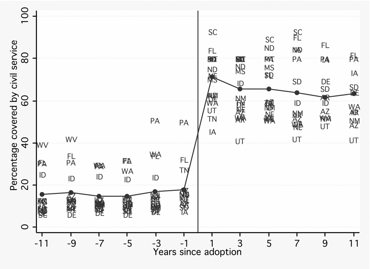
Figure 2 makes it clear that these partial reforms were quite limited in scope. For each state that passed a general civil service law after 1960, we calculated the percentage of full-time state employees covered under the state's civil service for the 11 years before and after the passage of the law.Footnote 12 Figure 2 shows these percentages as well as the average (the solid line). On average, prior to the passage of a general civil service law, less than 20% of the state employees were covered by civil service systems. After the passage of such a law, this jumped to an average of more than 60%.
The Share of Workers Covered by Civil Service Provisions as a Function of Years before and after a State's Passage of a Comprehensive Civil Service Reform

The scattered evidence available suggests that the states that passed general civil service laws before 1960 also exhibited a substantial increase in the percentage of employees covered under civil service after the reforms were passed. The 1905 civil service law in Wisconsin covered about 52% of state employees in 1908 and 63% in 1918; the 1921 law in Maryland covered about 69% in 1925; the 1908 law in New Jersey covered about 80% by 1922; the 1937 law in Arkansas covered about 67%; the 1937 law in Michigan and the 1939 law in Rhode Island both covered more than 80% in 1940; the 1939 laws in Alabama and Minnesota each covered about 80%; and the 1940 law in Louisiana covered about 85% of state employees. All of these represented large changes, because the baseline coverage rates were zero.
Figure 2 shows that in most states, the percent of employees covered is almost a step function, rising sharply with the passage of a general civil service reform. In a few states the expansion of the civil service was more gradual. For example, in Pennsylvania, the first law passed soon after the Social Security Act mandate mentioned previously. The governor extended the civil service by an executive order in 1956, adding about 13,000 positions and bringing the percentage of state employees covered to about 40% by 1961. In 1963 the state passed a major reform that increased the percentage covered to over 50%.
The exisiting literature focuses on four main arguments to explain why civil service reforms would be adopted: (1) shifting societal demands for public versus private interests and the success of progressive antimachine groups/politicians; (2) increasing transaction costs of managing patronage machines; (3) rising private sector wages that made patronage jobs undesirable; and (4) increasing political competitiveness raising the costs of the patronage system.Footnote 13 This fourth explanation is a potential concern for our identification strategy, which assumes that the reforms are exogenous to electoral outcomes. However, in the Specification section, we discuss why the research design we employ addresses some of the potential biases that could arise from a correlation between civil service reform and secular trends in political competition.
Like most “good government” laws, comprehensive civil service reforms were rarely repealed after being adopted. In a few rare incidents the “dominant” party, or a faction of it, repealed or weakened the reform.Footnote 14 In the analyses that follow we consider a state as having a comprehensive civil service law only after the “permanent” reform went into effect. There are several plausible explanations for the rare incidence of repealed civil service reforms. First, as noted, it seems generally difficult to retract legislation that is associated with “clean” government. This is also true for many of the progressive reforms that were enacted around the turn of the 20th century—e.g., the Australian ballot, direct primaries, and direct election of Senators. These were almost never retracted, even though they often did not obviously favor incumbents. Another plausible explanation is that the reform creates an interest group of civil service workers that strongly oppose repeal (e.g., Johnson and Libecap Reference Johnson and Libecap1994).
Hatch Act and Collective Bargaining
During the period when states were introducing civil service reforms, the Hatch Act amendment and public sector collective bargaining were also introduced. The Hatch Act in particular is widely perceived to have limited the ability of politicians to exploit patronage appointments for electoral gains. We include variables to capture the Hatch Act amendment and public sector bargaining in the analyses in the Robustness Checks section, to make sure that we do not incorrectly attribute any increase in political insulation of state employees that resulted from these measures to the introduction of civil service reform. In this section we briefly discuss how both of these measures could have significantly weakened the use of state patronage for electoral purposes.
The Hatch Act, which prohibits federal government employees from engaging in certain political activities, was amended in 1940 to extend the provisions of the Act to any state and local government employees who work in areas financed by federal government loans or grants.Footnote 15 State and local employees covered by the Hatch Act may not run for public office in partisan elections, use their official authority to interfere with or affect the results of an election or nomination, or directly or indirectly coerce contributions from subordinates in support of a political party or candidate. They are allowed to run for public office in nonpartisan elections, campaign for and hold office in political clubs and organizations, actively campaign for candidates for public office in partisan and nonpartisan elections, and contribute money to political organizations and attend political fundraising functions.Footnote 16
In principle, the Hatch Act would have constrained the use of patronage for electoral gain in states that had not yet adopted general civil service reforms by 1940. Whether the Hatch Act amendments were successful in limiting state employees' electioneering activities is not clear. Many scholars argue that violations of the Hatch Act were common. McKean (Reference McKean1949, 322–23) writes,
[I]t does not take much acquaintance among politicians to discover that they [the Hatch Acts] are widely evaded or violated. . . . In a vast variety of subtle ways it is possible for an employee to use his official discretion to influence elections, and he can covertly take a fairly active part in politics. . . . Some states have “Little Hatch Acts,” and others have provisions in their civil service laws to the same effect. Like the federal statutes, these too are often evaded and violated.
States sometimes choose to pay fines rather than dismiss employees for violations of the act. For example, Utah paid $42,000 in fines in 1960 rather than fire three employees of the State Highway Department for urging department employees to contribute to a Republican fund-raising dinner (Gordon, Richardson, and Williams Reference Gordon, Richardson and Williams1962).
Public sector collective bargaining may have also weakened the ability of politicians to use state patronage for electoral gains. The introduction of collective bargaining, especially provisions in labor contracts that specified procedures for terminating state employees, meant that politicians were more constrained in their ability to require that state government employees work for or contribute to the party as a condition for their employment. States introduced public sector collective bargaining provisions in the latter half of the 20th century, which is in most cases after they had already introduced civil service reforms. Klingner (Reference Klingner, Kellough and Nigro2006) notes that collective bargaining only “began in earnest in the public sector in 1960s and 1970s.”Footnote 17 In a few cases, however, collective bargaining agreements predated general civil service laws; and in other cases they may have strengthened the effects of these laws (Kramer Reference Kramer1962).
Why Focus on State Legislatures?
As noted earlier, in the main analyses (in Results), when defining partisan control of state government, we focus on control of state legislatures. In supplemental analyses (discussed in Robustness Checks), we explore alternative and more complicated definitions of control that include the governor and other elected statewide executive offices. In this section, we provide theoretical arguments that help justify our decision to focus on the state legislatures in our main analysis.
Ideally, we would like a measure of control that incorporates two factors: (1) who has the strongest influence over patronage appointments; and (2) who has the strongest incentives to use these appointments for electoral gain.
Regarding the first factor, officials in the executive branch typically have formal authority over appointments and dismissals of state government employees. However, in all states, the legislature holds the ultimate power to make all laws, and the legislature also holds the power of the purse. Thus, all other state officials must bargain with the legislature to get anything done. This fact is noted and discussed most frequently with regards to gubernatorial leadership—how governors obtain, or fail to obtain, legislative approval of their policy agendas. Zink (Reference Zink1951, 775) lays out the logic clearly:
It is very difficult for a governor to carry through a very ambitious program of legislation in most states without making some use of the patronage power. If a different type of person is elected to the legislature at some future time it may not be necessary to resort to offering jobs, promising political advancement and otherwise dangling favors before the eyes of those who make the laws. But under the present setup, the majority of those who get themselves elected to the seats in a state legislature expect to be rewarded for their services beyond the salary and honor attached to their office.
In a similar vein, Jewell (Reference Jewell1962, 120) states that “In most states the dispensing of jobs offers the governor one of his best opportunities to influence legislators; this is more important to most governors than to the President.” Nixon (Reference Nixon1948, 417) writes, “A governor bent on such a purpose [influencing the legislature] must make use of large amounts of both wisdom and patronage to succeed.”Footnote 18
Regarding the second factor—the incentives to use patronage to win elections—for most of U.S. history individual state legislators did not have the resources to run “personal” reelection campaigns, and were forced instead to rely on the party organization and the popularity of prominent party leaders. Even today this is true in many states. Legislators therefore have a strong incentive to use patronage for partisan electoral gain. Keefe (Reference Keefe and Heard1966, 45–46) writes,
Few matters have more intrinsic interest for legislatures than matters of personnel. For one thing, policy may be at stake. . . . More important, usually, is patronage. Where state merit systems are comprehensive, legislatures may see the civil service as a vast wasteland. But when jobs can be made available for supporters, legislative interest runs high; access to patronage may prove to be a critical resource in the life of the legislator.
Moreover, in the era of strong party organizations, most observers emphasized the importance of county organizations, and state legislators tended to have close ties to their counties.Footnote 19 The result, at least for a state with enough desirable patronage jobs, is predictable: “The patronage agency, then, is under continuing pressure by the county chairmen and some state legislators for jobs and is always well supplied with applicants for certain kinds of positions. The problem faced by the patronage administrator, therefore, is how to allocate his resources in the face of demands placed upon him” (Tucker, Reference Tucker1969, 82). Merriam and Gosnell (Reference Merriam and Gosnell1949, 211) echo this assessment, especially with respect to nonurban machines: “The rural boss system is based chiefly upon patronage and minor spoils of various types, and it connects with the state organization through the state legislature, where votes are needed.”Footnote 20
Finally, incorporating the executive branch in measuring partisan control over patronage is complicated because of the “plural executive.” Governors did not have monopoly control over all appointments. In most states during the period we study, the lieutenant governor, secretary of state, attorney general, treasurer, auditor or comptroller, and public school superintendent were typically separately elected officials. In many states one or more of the following commissioners were also elected: public utilities, agriculture, insurance, state lands, mines, taxes, highways, and public works. In some states administration was further decentralized by the existence of numerous independent boards or commissions, whose heads were chosen by the governor with the consent of the state senate, or in some cases directly by the legislature (i.e., the “New Jersey Plan”). Prior to the adoption of the civil service law, these officials often controlled the patronage jobs under their administration and bargained separately with the legislature in the allocation of this patronage. Carpenter and Stafford (Reference Carpenter and Stafford1936, 49) note that “The governor is seriously handicapped by the dispersion of executive power among constitutional officers, over whose appointment and removal he seldom has any control.”Footnote 21 We attempt to address this complex division of authority in our supplemental analysis by including partisan affiliations of elected downballot statewide executives in our measure of party control of state government.
THE EFFECT OF PATRONAGE ON ELECTION OUTCOMES
Specification
As noted earlier, under a patronage system the party that wins control of government should be able to use patronage to win future elections. We assess this prediction empirically by asking the following questions. Suppose that a party wins control of the legislature in state s in the election at time t. What is the probability that this party continues to control the state legislature by winning the elections at times t + 1, t + 2, t + 3, and so on? Is this probability higher if state s is under a patronage system rather than a civil service system?
A party controls the legislature after an election at time t if it holds majorities in both houses. If control is split across the houses, or if there is an exact tie in one house and the major legislative positions were divided, then neither party controls the legislature at time t. These cases are dropped from the analysis. Our basic specification is simple:

The dependent variable V st is the future election outcome under study from the point of view of the party that controls the legislature in state s at time t. The main variable of interest is P st, a dummy variable defined as P st=1 if state s is operating under a patronage system at time t and P st=0 if state s is operating under a general civil service law. The variable M st captures the size of the majority party's strength among voters at time t. The αs's and γt's are state and year fixed effects, respectively.Footnote 22
The majority party's underlying strength, M st, is a function of many factors including the distribution of partisanship among voters, the effects of gerrymandering and malapportionment on the mapping between votes and seats, and valence advantages for majority party candidates. Thus, to measure M st, we use the share of lower house seats won at time t by the party controlling the state legislature at time t, minus 50%.Footnote 23 We focus on the lower houses because they are relatively large, with a median size of 100 seats. Also, almost all lower houses have two-year terms in which all seats are up for election every two years.Footnote 24 By contrast, upper house seat shares are a relatively noisy measure of majority party strength. Upper houses are small, so seat shares are lumpy—the median number of seats in our sample is only 35 and the average is 37. Moreover, in most states upper houses have staggered four-year terms, with only half of the seats up for election every two years. Thus, it may easily be the case that the particular seats up for election in any given year are not representative of the state as a whole.
We should emphasize that although our measure of majority party strength, M st, is constructed using the lower house only, our measure of majority party control in each state and each period is based on control of both houses.
There are two additional concerns regarding the functional form in equation (1). First, because the dependent variable V st is dichotomous, the relationship between V st and M st is probably nonlinear. To capture this, in some specifications we set k > 1.
Second, it is likely that the relationship between V st and patronage, P st, varies with M st. In particular, we expect the effects of patronage on winning future elections to be larger when M st is smaller. In a state where political competition is lopsided because of the distribution of voter partisanship and other factors—e.g., a southern state before 1964 with a disproportionate number of loyal Democratic voters, or one of the northern states before 1930 with a disproportionate number of loyal Republicans—the dominant party will win at time t, and at times t + 1, t + 2, etc., regardless of whether or not they have access to patronage. In more competitive situations, however, where both parties have a reasonable chance of winning, control of the patronage apparatus may make a difference.
We deal with this second concern in three ways. First, we drop all extremely lopsided cases, in which the majority party won more than 80% of the seats in either the lower or upper house. These are cases where we expect the effect of patronage to be near zero. Moreover, adding these cases could potentially increase bias if we did not make additional adjustments to the functional form, which are likely to reduce efficiency. If we add the lopsided cases, estimates imply that the effect of patronage on winning future elections is even larger than what we report later—i.e., our estimates of β1 are even larger than what we report later. Second, in equation (1), we allow the effect of patronage on V st to vary with M st. This is captured in the ∑k=1K β3kP stM stk term.
The third approach to dealing with this heterogeneity, which is our preferred approach, is to focus on cases where the majority party in state s at time t was determined by a relatively close election.Footnote 25 These are the cases where we expect patronage to matter the most.Footnote 26 Because we use narrow windows to define close elections, we do not include state fixed effects, year fixed effects, or lower house seat share in these specifications.
If β1>0, then the party controlling the legislature at time t is more likely to win subsequent elections under a patronage regime than under the civil service when the lower house is evenly divided.Footnote 27,Footnote 28
We study four dependent variables: (i) a dummy variable indicating that the party in control at t also won control of the state legislature in each of the subsequent eight years beginning at t + 1; (ii) the share of statewide offices won by the party in control at t during the eight years beginning at t + 1; (iii) a dummy variable indicating that the party in control at t won control of the state legislature in the subsequent four years beginning at t + 1; and (iv) the share of statewide offices won by the party in control at t during the four years beginning at t + 1. The first two variables capture relatively long-term effects. We use an eight-year window because most upper houses in state legislatures have four-year terms and most statewide offices are four-year terms—thus, for most states the variables cover two full election-cycles. Also, variable (i) captures four lower-house elections. The second two variables capture more short-term effects—typically, one full election cycle in the state legislature and the next election of statewide officials.Footnote 29
We study the period from 1885 to 1995. Because there may be important changes in the political structure right before and after the civil service reforms, we exclude the six years directly before and after the adoption of the general civil service reform law in each state.Footnote 30
As equation (1) makes clear, our strategy for identifying the effect of patronage is a differences-in-differences approach, exploiting the fact that different states adopted general civil service reforms at different times.
Of course, this approach rests on the assumption that the timing of civil service reforms is exogenous to expected future election outcomes. Although many of the existing explanations for the reforms do not rely on factors explicitly linked to future electoral outcomes, some recent explanations discussed earlier do link the introduction of civil reforms to increasing political competition in the years leading up to the reforms.
Thus, an association between the introduction of civil service reforms and the length of partisan control of state legislatures may simply be capturing a trend toward increasing political competition that is independent of the reforms. When a state's elections are not competitive, we would naturally expect the same party that wins control of the state legislature in any given election to remain in control as long as elections remain uncompetitive. If elections in this same state become competitive, then we naturally expect a decline in the probability of a party continuing to control the legislature in future elections. Thus, even if civil service reforms were exogenous and political competition were increasing over time, we would expect to observe a stronger correlation between winning control of the state legislature in a given election and future control of the state legislature under a patronage system as compared to a civil service system.
Four aspects of our research design address this concern. First, we exploit the variation in when states introduced civil service reforms and include year fixed effects in order to avoid biases that may arise from trends in political competition common to all states. Second, we attempt to control for the majority party's strength in each year by including M st in our specifications, either in a linear or in a polynomial form. Thus, even if different states became competitive at different times, and if the reforms were endogenous to the level of competition, the M st terms should help account for potential trends in political competition.
Third, we focus on cases where parties win control of the state legislature by narrow margins. This makes the set of state–year cases pre- and post-civil service reform more comparable—i.e., the samples of state–years identified as close cases are politically competitive in both periods. To test whether the pre and post cases have similar levels of political competition, we examine whether there is a significant difference in the normal vote in state–year cases used in our analysis. We measure the normal vote using all available statewide offices plus the U.S. Senate and President. For each state and year, we compute the average of the two-party vote share for all available races from the point of view of the party in control of the state legislature. The difference in this normal vote between the pre- and post-reform periods is neither substantively nor statistically significant.
Finally, we exclude elections a few years before and after the reforms. State politicians may have been responding to short-term changes in political competition in the years leading up to the reforms. This could bias toward finding a relationship between patronage and electoral outcomes if there is a sharp decline in political competition in the years leading to and following the introduction of civil service reforms. If the party that passes the reform also receives an electoral bonus, then this could actually bias away from finding a relationship beween patronage and control of state government.
Results
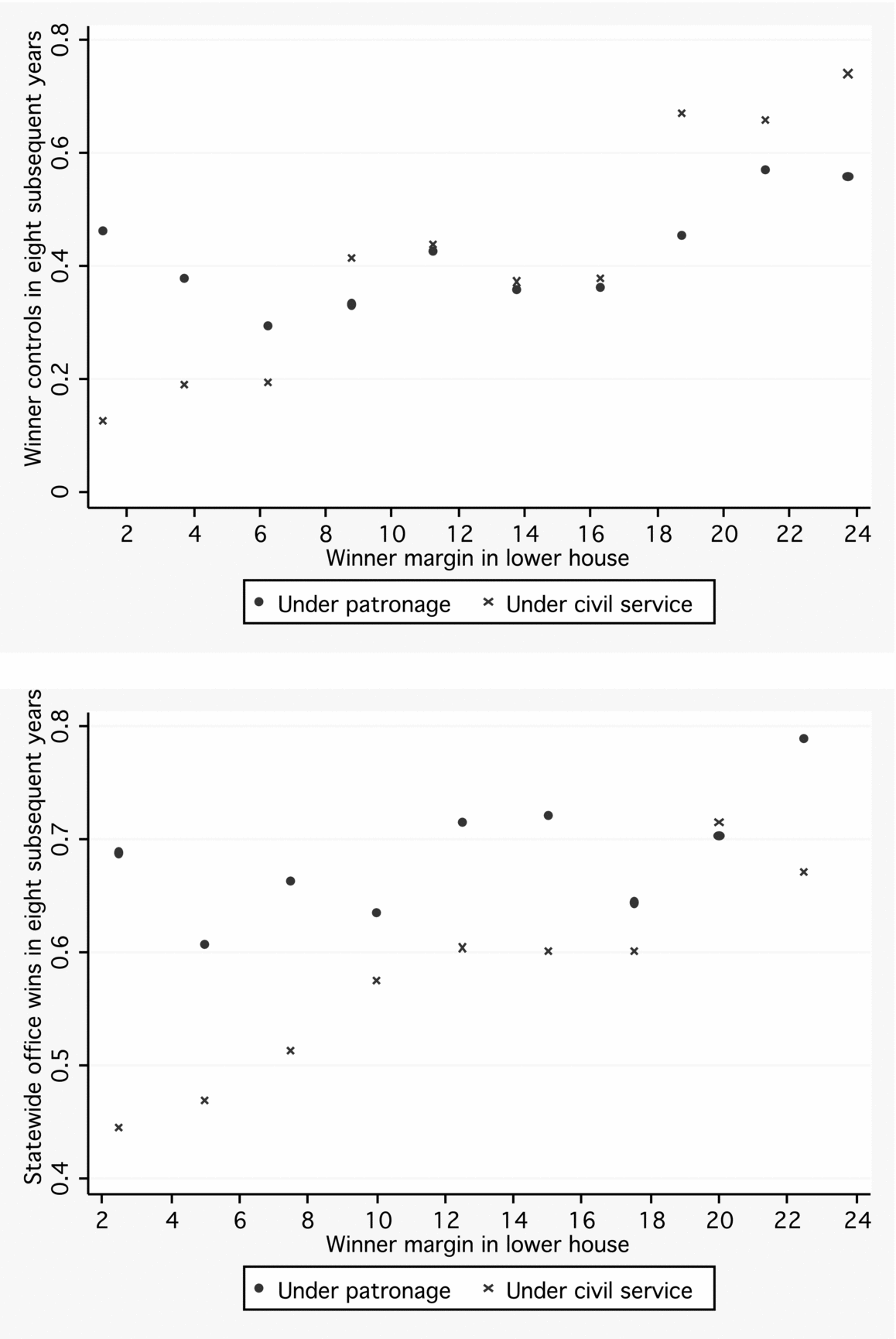
We begin with a graphical analysis, shown in Figures 3a and 3b. These figures show binned averages of two outcome variables as a function of the winning party's margin in the lower house at time t. The outcome variable in Figure 3a is an indicator for whether the party that controlled the legislature at time t also won control of the state legislature in each of the subsequent eight years (four elections) beginning at t + 1. The outcome variable in Figure 3b is the share of statewide offices won by the party in control at t during the eight years beginning at t + 1. The figures show that winning full control by winning the lower house had a different effect on future electoral success for elections before and after the introduction of civil service reforms. Note that in both figures, for the bins closest to the threshold, which cover margins of 0 to 7%, the incumbent party always does better under a patronage system than under a civil service system. This is consistent with the main predictions discussed earlier. In Figure 3b the incumbent party does better under a patronage system even for a broader range of margins.
(a) Binned averages of the share of parties maintaining full control of the legislature for 8 subsequent years as a function of the win margin in the lower house. (b) Binned averages of the share of wins statewide elections during 8 subsequent years for the party in full control of the legislature as a function of the win margin in the lower house. The win margin is defined in seat share. The bandwidth is 2 percentage points.

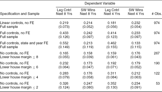
Table 1 presents the main regression results. Each column corresponds to one of the four dependent variables described earlier. The top panel studies the full sample. The rows in this panel show specifications with different sets of regressors. The bottom panel only uses observations where the winner at t won the lower house by a fairly close margin. Each row corresponds to a different threshold for determining close elections. Each entry shows the estimated coefficient on Patronage Dummy, i.e., β1 from equation (1), with the estimated standard error below in parentheses. The number of observations is shown in the last column.
Patronage and Election Outcomes 1885–1995

Notes: Each column presents estimates of the coefficient on the Patronage variable with the dependent variable listed at the top of each column. Rows (1)–(3) present estimates of β1 from equation (1) including both close and non-close elections. Rows (4)–(7) present estimates of the coefficient on the Patronage variable focusing on close elections. The estimates in row (1) include the Margin variable and the Margin variable interacted with the Patronage variable. Rows (2) and (3) include a third-order polynomial of the Margin variable as well as its interaction with the Patronage variable. Row (3) also includes state and year fixe deffects. Robust standard errors are in parentheses. In rows (1)–(3) the standard errors are clustered by state.
To see what the coefficients mean, consider, for example, the first column and sixth row. The point estimate of 0.28 implies that when the winning party of a lower house election at t has a seat share advantage of four percentage points or less, the probability that the winning party continues to control the state legislature over the next eight years is about 28 percentage points higher under patronage than under the civil service.
In virtually all cases, the estimated coefficient on Patronage Dummy is statistically significant and substantively large, with the point estimates ranging from about 0.16 to about 0.34 in the bottom panel. Note also that in all columns, the estimated coefficient on Patronage Dummy falls as the threshold used to define close races increases—i.e., as increasingly lopsided cases are added. This probably reflects the fact that we are adding cases where one party has a nontrivial advantage in voter loyalty, so patronage per se is less important for winning. Importantly, patronage is correlated not only with future legislative victories, but also with winning control of statewide offices (columns (2) and (4)). This is important because it indicates that the coefficients for the legislative dependent variables do not simply capture an effect of gerrymandering or malapportionment. Statewide offices are, by definition, not districted, so they cannot be gerrymandered or malapportioned.Footnote 31
Overall, then, the results in Table 1 are consistent with the hypothesis that parties were able to use patronage to help win elections. As expected, the estimated coefficient on Patronage Dummy is largest when comparing cases where state legislative election outcomes are close.
Robustness Checks
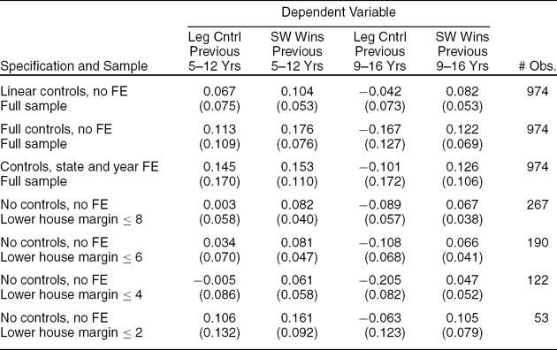
Table 2 presents a set of “placebo” tests. The structure is the same as in Table 1, but the dependent variables refer to elections prior to the election at time t, rather than elections after time t. Winning at time t should have no systematic causal effect on winning prior to time t. In the first two columns of the table the dependent variable is defined in terms of legislative control (column (1)) or statewide office victories (column (2)) that occur between years t − 12 and t − 5. In columns (3) and (4) of the table the dependent variables cover control and victories for years t − 16 and t − 9. Note that we do not include the most recent past—i.e., years t − 5 and t − 1—because we use these years to define “entrenched parties” in the analyses that follow.
Placebo Regressions

Notes: Each column presents estimates of the coefficient on the Patronage variable with the dependent variable listed at the top of each column. Rows (1)–(3) present estimates of β1 from equation (1) including both close and nonclose elections. Rows (4)–(7) present estimates of the coefficient on the Patronage variable focusing on close elections. The estimates in row (1) include the Margin variable and the Margin variable interacted withthe Patronage variable. Rows (2) and (3) include a third-order polynomial of the Margin variable as well as its interaction with the Patronage variable. Row (3) also includes state and year fixed effects. Robust standard errors are in parentheses. In rows (1)–(3) the standard errors are clustered by state.
The estimated coefficients in Table 2 are uniformly lower than those in Table 1 and some are even negative, and none are statistically significant at the standard 5% level. A few of the coefficients are large—e.g., those in the last row of columns (1) and (2)—but we take comfort in the fact that the estimates are relatively unstable as we move from row to row within columns. In particular, none of the columns have consistently large coefficients. Thus, overall these results increase our confidence that the estimates in Table 1 are not just picking up something spurious—e.g., differential changes in voter partisanship across states that are correlated with civil service reform.
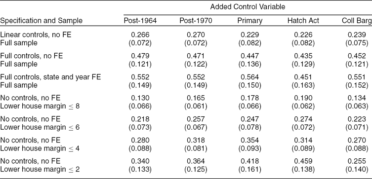
We also ran the previous regressions including five additional variables. The first variable captures the “reapportionment revolution” due to Baker v. Carr and related Supreme Court decisions. Malapportionment is one potentially easy way for a party to remain in power—it can create state legislative districts such that the areas where the supporters of the opposing party tend to live are underrepresented and the areas where its supporters live are overrepresented. The decision in Reynolds v. Sims (1964) made this practice illegal. We measure this simply with a post-1964 dummy variable. This variable also effectively captures the era of the “personal incumbency advantage.” If individual incumbents have a large personal advantage, then the party that wins more seats at time t may continue to win at time t + 1, etc. simply because it has more incumbents, each of whom has a personal advantage. Most previous work finds a large personal incumbency advantage emerging by the late 1960s.Footnote 32 The second variable captures direct primary elections. Many progressive reformers argued that the direct primary would weaken the party machines. Under primaries, machine leaders would no longer have control over nominations, so that aspiring politicians would no longer be forced to work for the machine. We measure this with a dummy variable that is 1 for years when a state had mandatory primary elections and 0 otherwise. The third variable is an indicator for pre- and post-Hatch Act adoption and prior to civil service reform. As discussed previously, the Hatch Act may have had a dampening effect on the use of patronage by prohibiting certain state employees from engaging in election-related activities.Footnote 33 Finally, we include a dummy variable for the introduction of provisions allowing collective bargaining by public sector employees.Footnote 34
We present the results of these analyses in Table 3. In none of these cases does the additional variable substantially affect the estimate of the coefficient on the Patronage Dummy variable. The coefficient on Patronage Dummy remains statistically significant in virtually all specifications, and the additional variable is never large or statistically significant itself.
Including Additional Control Variables

Notes: Dependent variable: Legislative Control, next eight years. Each column presents estimates of the coefficient on the Patronage variable including an additional control variable listed at the top of each column. Rows (1)–(3) present estimates of β1 from equation (1) including both close and non-close elections. Rows (4)–(7) present estimates of the coefficient on the Patronage variable focusing on close elections. The estimates in row (1) include the Margin variable and the Margin variable interacted with the Patronage variable. Rows (2) and (3) include a third-order polynomial of the Margin variable as well as its interaction with the Patronage variable. Row (3) also includesstate and year fixed effects. Robust standard errors are in parentheses. In rows (1)–(3) the standard errors are clustered by state. See Table 1 for sample sizes.
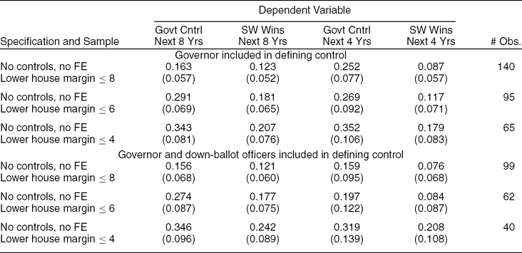
A further robustness check is to consider alternative definitions of state government control, especially definitions that include control of the governor's office and statewide offices. We estimate the baseline specification limiting the sample to those observations in which the party controlling the legislature also holds the governorship. We then further limit the sample to observations where the party controlling the legislature holds two thirds of the elected statewide executive offices in addition to the governorship. The results are presented in the Appendix, Table A.1. The estimated coefficient on Patronage Dummy is positive and statistically significant in all but two cases. In fact, in most specifications the estimate is even larger than the analogous coefficient in Table 1, although the differences are quite small.
ENTRENCHED VERSUS NONENTRENCHED PARTIES
In this section we examine whether the electoral advantage from controlling the legislature under a patronage system is larger for parties with recent experience as the majority party. We refer to parties that have been in power continuously for a disportionate portion of the years prior to an election as entrenched parties. Although some scholars, such as Sorauf (Reference Sorauf1959), might find the claim that entrenched parties will have an additional electoral advantage under a patronage system as being intuitive and perhaps even obvious, the rationale underlying this claim is often not clearly articulated and, at least to our knowledge, there is no systematic evidence that this entrenched party advantage exists. Thus, we begin by discussing some of the factors that could lead entrenched parties to have an electoral advantage under a patronage system. We then present the specification and results.
Theoretical Considerations
An entrenched party typically enjoys an intrinsic electoral advantage over its opponents, because of factors such as imbalance in the distribution of ideological positions, policy preferences, or party attachments among voters. Although this intrinsic advantage exists under both patronage and civil service systems, we present four factors that could theoretically provide entrenched parties an electoral advantage under a patronage system relative to nonentrenched parties.
First, entrenched parties are likely to have a monetary resource advantage over other parties under a patronage system. By definition, an entrenched party will tend to be in power more often than other parties. If party organizations can extract part of their patronage appointees' salaries, then an entrenched party will be able to accumulate these resources over a longer time period compared to the weaker party.Footnote 35
Second, entrenched parties are more likely to attract high-quality employees—specifically, employees with electioneering talent. Suppose that the entrenched party is in power, say, 75% of the time, whereas the weaker party is only in power 25% of the time. In this situation the expected value of the same wage—the wage of the government job times the probability of holding the job—is three times as large when offered by the entrenched party as compared to the weaker party. So, when bidding for talented workers, the entrenched party should win against the weaker party most if not all of the time.
Third, entrenched parties under patronage will benefit from having more opportunities for on-the-job learning. Electioneering is labor-intensive, and effective party workers must develop networks of friends and acquaintances who can be persuaded to vote for the party and, in some cases, to donate time and money to get others to vote. Developing and maintaining these networks, and learning effective tools of persuasion, takes time and effort. Because the entrenched party is in power more often than other parties, its workers should have larger stocks of human capital than workers of other parties. Furthermore, to the extent that acquiring electioneering skills is costly, supporters of the entrenched party have a stronger incentive to acquire such skills, as they tend to have more opportunities to actually use this capital.
Finally, another human capital–related reason entrenched parties may benefit from patronage is that their appointees are likely to have acquired more experience in providing government services. Again, by definition, the entrenched party is in power more often than other parties, so under the patronage system its workers will, on average, have acquired more on-the-job human capital than those of the weaker party. To the extent that this experience leads to better provision of government services, voters may have a preference for the appointees of an entrenched party.
We must note one caveat. It is not obvious that the marginal benefits of winning the election at time t—which is the quantity we estimate—are monotonically increasing in the amount of time that an entrenched party has been in power. For example, a party that has been entrenched for a long period of time may have accumulated enough resources from the partisan state employees that losing control for one term may have a smaller impact on its future reelection chances. In addition, a party that has been out of power for a long period of time and suddenly finds itself in office may have difficulty removing the entrenched party's workers without losing significant amounts of human capital.
Specification Issues
For each state s, and each time t, a party is considered to be entrenched if it held control of the legislature in state s for several consecutive years prior to t. We use three different criteria for classifying a party as entrenched: (1) full control of the state legislature during the prior two years; (2) full control during the prior four years; (3) full control during the prior six years. In all cases we use the same criterion for classifying a party as nonentrenched, which is that the party was not in control of the state legislature in the year prior to the election at time t.Footnote 36
Earlier, we found that the electoral advantage from legislative control in patronage systems is most pronounced when “close” elections are examined. Thus, in this analysis, we focus on cases where the seat margin in the lower house election in state s at time t was relatively small. We employ the same specification used to estimate the coefficients in the lower panel of Table 1, but now we include a dummy variable for whether the party that wins the election at time t is entrenched and an interaction term between this dummy variable and the Patronage Dummy variable. The results using the full sample and a specification similar to equation (1) are substantively very similar to our findings focusing on close elections.Footnote 37 Our specification is

where V st is the election outcome under study from the point of view of the party that controls the legislature in state s at time t. I st is the Entrenched Party Dummy, which is equal to 1 if the party winning control of the legislature in state s at time t also controlled the legislature for the previous four years and 0 otherwise. P st is the Patronage Dummy variable, which is equal to 1 if state s is operating under a patronage system at time t and 0 otherwise. Note that β2 is the relative electoral advantage enjoyed by the entrenched party from holding a majority of the seats in house j at time t, compared to the advantage enjoyed by a nonentrenched party under the civil service system.Footnote 38 The main parameter of interest, β1, is the relative electoral advantage enjoyed by the entrenched party under the patronage system, which helps us capture the relative advantage versus both entrenched parties under civil service, β2, and nonentrenched parties under patronage, β3.Footnote 39 Given the arguments in the previous section, we expect β1 to be positive.
The dependent variables are the same, as is the time period studied. We run the regressions in the subsample of close lower house elections. The limits in winning margin we use to define close elections are 4, 6, and 8%. The reasons for focusing on this subset of elections were discussed previously.
Results
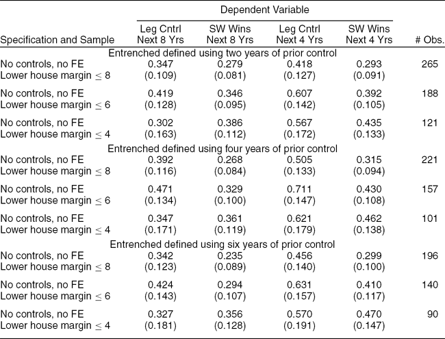
The results are shown in Table 4, which is similar in format to the lower panel of Table 1. As noted earlier, we only use observations where the winner at t won control of the lower house by a close margin. There are three panels, one for each way we define entrenched parties. The coefficients presented are the estimates of β1 from equation (2), i.e., the coefficients on the interaction term between the patronage and the entrenched party dummy variables.
Entrenched versus Unentrenched Parties

Notes: Each column presents estimates of the coefficient on the Patronage variable interacted with the Entrenched variable with the dependent variable listed at the top of each column. Rows (1)–(3) present estimates of β1 using 2 years of full legislative control to define entrenched parties. Rows (4)–(6) present estimates of β1 using 4 years of full legislative control to define entrenched parties. Rows (7)–(9) present estimates of β1 using 6 years of full legislative control to define entrenched parties. Robust standard errors are in parentheses.
The results in Table 4 show that the difference in the probability of winning future elections between states under patronage and civil service largely reflects the advantage for entrenched parties under patronage. The estimated coefficient on the interaction term between the Patronage Dummy and the dummy for the entrenched party winning control at time t is substantively large and in all but one case statistically significant. Consider, for example, the results in the middle panel, i.e., using four years of prior control to define entrenched parties. In the specification where we use the 6% percent threshold to define close elections and estimate the probability of maintaining control for the eight subsequent years, we find the point estimate of β1 to be 0.47. This implies that the probability of maintaining control of the state legislature under patronage is about 47 percentage points higher for an entrenched party than for a nonentrenched party. Overall, the estimates of β1 are largest when we use the four years of prior control definition, but they are not significantly different.Footnote 40 If anything, this suggests that the marginal impact of an extra term of control is not monotonically increasing in the number of years of prior control.
We do not include the estimates of the main effects, i.e.,  2 and 3, in Table 4 to conserve space. The estimates of the coefficient on the Patronage Dummy variable are not statistically significant in any specification. The estimates are also significantly different from the coefficient on the interaction term in almost all specifications. This indicates that the nonentrenched parties did not significantly benefit from control of government under the patronage system, which is consistent with the theoretical arguments regarding why entrenched parties would be the main beneficiaries from a patronage system.
Entrenched Party Advantage in Close Elections under Patronage
We suspect that patronage is likely to be a particularly valuable resource for parties when there is a threat of losing an election. Thus, if patronage provides entrenched parties with an electoral advantage, we might expect to observe a difference in the fraction of close elections they win before and after the introduction of general civil service reforms. The fraction should be smaller under the civil service system. To examine whether such a pattern exists, we compute the share of close election wins for entrenched parties under patronage versus civil service. We examine this for five winning margins in the lower house—one, two, three, four and five percentage points.
Note that in general we expect some sorting in favor of entrenched parties, except for very small windows around 50%. This is simply because entrenched parties, on average, are likely to have more voter support. Suppose, for example, that the Democratic seat share in a state is normally distributed around 60%. Then there will automatically be more elections in the 50–55% window than in the 45–50% window. However, although we expect to see some sorting, we do not expect to see a large difference in entrenched parties' win margins between patronage and civil service regimes.Footnote 41
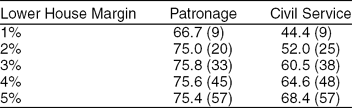
Table 5 shows the share of wins in close elections. Under patronage, the share of wins for the entrenched party remains constant at about 75%. That is, the entrenched party is expected to win three out of four elections even when the elections are very close. Under civil service the entrenched parties have no advantage in winning very close elections. However, as expected, the share of wins does increase as we increase the margin defining closeness. Thus, the anomaly is that the share of wins remains constant and high under patronage as we narrow the window for close elections. We also compared the share of wins in close elections for nonentrenched parties, and we do not find any electoral advantage in close races, under either patronage or civil service. If anything, parties with one term of legislative control tend to lose more close elections than they win under patronage. Given the small sample sizes, we cannot draw any clear conclusions, but the pattern is very different from that for the entrenched parties under patronage.
Sorting in Close Elections, 1885–1995

Notes: Each column presents the share of wins for the entrenched party in close elections. Each row represents a different definition of close election. The number of close elections under each definition is shown in parentheses. Only cases when there is an entrenched party are included in the sample. Entrenched parties are parties with four years of full legislative control.
These results are consistent with the idea that parties in control of patronage machines are able to turn on the party machine to win close elections and maintain legislative control. Turning on the party machine could imply two things. One is that the party is able to increase the amount of campaign resources raised when the election is expected to be close, and allocate these resources to key districts. Another possibility is electoral fraud—the party is simply cheating. We cannot determine which of these underlies the results in Table 5, or whether it is a mixture of both. We can say that entrenched parties were evidently no longer able to turn on the machine or engage in fraud to the same extent after the introduction of civil service.
CONCLUSION
Tammany Hall Boss William Tweed popularized the saying, “To the victor belongs the spoils” (Maranto and Johnson Reference Maranto, Johnson, Bowman and West2007). For much of U.S. history, patronage was one of the major “spoils” available to victorious political parties. Although some of these spoils were probably consumed as rents, some were probably used to maintain control of government—otherwise, parties would miss out on future spoils. One of the motivations for civil service reforms was to eliminate such concentrations of resources in the hands of incumbents. Despite this widespread perception, there has been little systematic evidence that political parties have been able to utilize their control over patronage for their own electoral advantage.
The main contribution of this paper is to provide quantitative evidence that control of patronage increases the probability that the incumbent party will win future elections. Prior to the introduction of state civil service reform, a party that won full control of the state legislature would significantly increase the likelihood of winning not only the next election but also several subsequent elections. This electoral advantage from controlling the state legislature was no longer present after states enacted legislation to expand the number of state employees covered under civil service.
Although our analysis points to civil service reform as a means of weakening partisan control of patronage, other changes occurring during our time period may also have potentially weakened the impact of patronage on electoral outcomes. In The Effect of Patronage on Election Outcomes section, we check the robustness of our findings against alternative explanations, such as the rising personal vote and the “reapportionment revolution.” We also examine the influence of two additional factors that may have affected the changing impact of control of the state legislature on future electoral success—the Hatch Act and collective bargaining by state employees.
Another contribution in this paper is to provide evidence that being an entrenched party yields additional electoral benefits from gaining control of patronage. We outline some theoretical reasons that the benefits from control of patronage may be related to the length of time the party is in power.
Finally, we also began to explore the mechanisms through which entrenched parties have an advantage over nonentrenched parties. This is another potential area in which we intend to extend our analysis. Clearly, however, much more work on mechanisms remains.Footnote 42
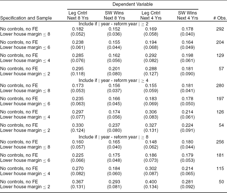
One potential concern with our analysis that we intend to investigate in future research is the nonrandom nature of when civil service reforms were enacted. If the civil service reforms were in part motivated by the changes in electoral outcomes, our estimates of the political impact of the patronage system could suffer from an endogeneity bias. Some preliminary robustness checks—e.g., limiting the sample to 30 years before and after the introduction of the civil service—provide little evidence that our findings simply reflect an underlying trend that affects both electoral outcomes and the timing of civil service reform. However, further analysis of the passage of state civil service reforms is necessary. Careful case studies would be especially useful at this point.
Our findings also provide some insight into why state party organizations have weakened over time. Our results are consistent with the idea that parties in control of the legislature may have used patronage to cultivate a loyal partisan electoral base. Civil service reforms which removed this core group of party supporters beholden to the incumbent party for their employment weakened the ability of political parties to organize their supporters within the electorate. Further investigation of this connection between civil service reform and the strength of party organizations is another area which we plan to explore in future research.
APPENDIX

Notes: Each column presents estimates of the coefficient on the Patronage variable for close elections with the dependent variable listed at the top of each column. In rows (1)–(3) the control of the state government is defined by controlling the legislature and governorship. In rows (4)–(6) control of the state government is defined as controlling both houses in the legislature, the governorship, and two/third of the elected state executive offices. Robust standard errors are in parentheses.

Notes: Cell entries are the estimated coefficients on the Patronage variable. Robust standard errors in parentheses.




Comments
No Comments have been published for this article.