Appendix 1: Additional Tables
The following tables present additional summary statistics and robustness checks for the article, “American Mobility and the Expansion of Public Education.” Descriptions of the data sources used for the article are given in Appendix 2. Appendix 3 presents a discussion of the effects of mismatches between the Iowa state census and the federal census when constructing the intergenerational data set used in the article.
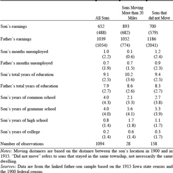
Appendix Table 1 provides summary statistics for the sons in the sample by distance moved. The purpose of the table is to assess the selection issues caused by losing the most geographically mobile individuals in the data construction process. The statistics in Appendix Table 1 reveal that the more geographically mobile individuals that remain in the data set tend to have higher incomes, more years of education, and fewer months of unemployment than their less geographically mobile counterparts. This suggests that the limitations of the linking process may lead to a data set that is underrepresentative of highly educated and successful sons. However, it should be noted that the differences in means between the highly geographically mobile sons and the stationary sons are quite small relative to the standard deviations of the variables within each group.
SUMMARY STATISTICS FOR THE IOWA SAMPLE BY DISTANCE MOVED BETWEEN 1900 AND 1915

Notes:
Moving distances are based on the distance between the son's location in 1900 and in 1915. “Did not move” refers to sons that stayed in the same township, not necessarily the same dwelling.
Sources:
Data are from the linked father-son sample based on the 1915 Iowa state census and the 1900 federal census.
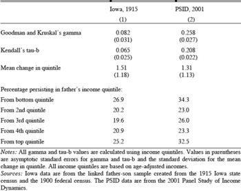
Appendix Table 2 presents several alternative measures of income mobility to supplement the intergenerational income elasticities in Table 2 of the article. As with the intergenerational income elasticity, these alternative measures all show greater income mobility in Iowa in 1915 than in modern times. Goodman and Kruskal's gamma and Kendall's tau-b are both measures of the number of concordant pairs relative to discordant pairs in the data.Footnote 1 A pair of observations A and B is concordant if the income of son A is greater than the income of son B and the income of father A is greater than the income of father B. A discordant pair would be a pair of observations A and B for which son A has a greater income than son B, but father B has a greater income than father A. A larger number of concordant pairs produces larger values for gamma and tau-b and is interpreted as less income mobility. Thus the significantly larger values of these measures for 2001 relative to 1915 suggests that the Iowa sample exhibits substantially more income mobility than the modern sample. The quintile measures show that sons were more likely to move larger distances in the income distribution in 1915 and that there was less persistance in each quintile of the income distribution in 1915, particularly in the bottom and top income quintiles. These results are consistent with intergenerational income elasticities in Table 2 of the article as well as the increasing persistence in the tails of the income distribution with improving school access and quality found in the logit estimates in Table 5 of the article.
ALTERNATIVE INCOME MOBILITY MEASURES

Notes:
All gamma and tau-b values are calculated using income quintiles. Values in parentheses are asymptotic standard errors for gamma and tau-b and the standard deviation for the mean change in quintile. All income quintiles are based on age-adjusted incomes.
Sources:
Iowa data are from the linked father-son sample created from the 1915 Iowa state census and the 1900 federal census. The PSID data are from the 2001 Panel Study of Income Dynamics.
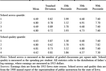
Appendix Table 3 addresses the issue of the endogeneity of school district characteristics. This table shows statistics of the father's income distribution by school district access and quality. Graded classrooms per square mile is used as a proxy for school access and spending per student is used as a proxy for school quality. The table reveals no discernible trends in the mean or variance of the income distribution by school district access or quality suggesting that the better school districts were not systematically located in richer communities.
SUMMARY STATISTICS FOR THE DISTRIBUTION OF FATHER'S LOG EARNINGS BY SCHOOL DISTRICT CHARACTERISTICS

Notes:
School access is measured as the number of graded classrooms per square mile. School quality is measured as the spending per student. All statistics refer to the distribution of father's log earnings, where earnings are measured in 1915 dollars.
Sources:
Earnings data are from the 1915 Iowa state census. School access and quality data are from the 1900 annual report of the superintendent of public instruction for the state of Iowa.
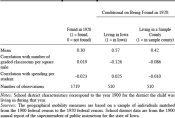
Appendix Table 4 examines whether the quality of a school district was correlated with the geographical mobility of its residents and consequently the likelihood of those individuals being successfully linked. The data for the table come from a random sample of individuals from the 1900 federal census living in the sample counties matched to the 1920 federal census. The probability of being found in 1920 was very weakly correlated with school quality and school access. The probability of still living in a sample county was negatively correlated with the number of graded classrooms per square mile and only very weakly correlated with school quality. These results suggest that communities with differing school quality did not have significantly different levels of geographical mobility, but that communities with better school access may have had more geographically mobile individuals. If more geographically mobile individuals also exhibit more income mobility, the marginal effect of school access on the intergenerational income elasticity estimated in the article will be overstated due to geographically mobile individuals being underrepresented in the sample.
CORRELATIONS BETWEEN GEOGRAPHICAL MOBILITY AND CHILDHOOD SCHOOL DISTRICT CHARACTERISTICS

Notes:
School district characteristics correspond to the year 1900 for the district the child was living in during that year.
Sources:
The geographical mobility measures are based on a sample of individuals matched from the 1900 federal census to the 1920 federal census. School district data are from the 1900 annual report of the superintendent of public instruction for the state of Iowa.
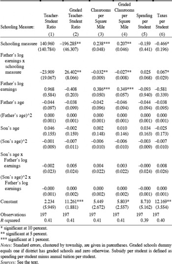
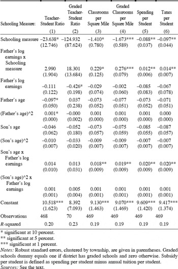
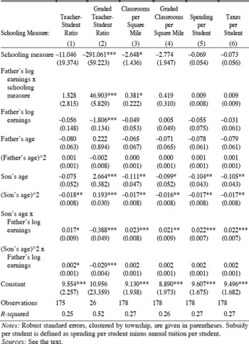
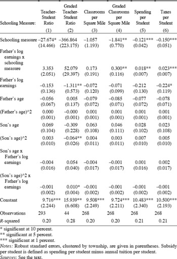
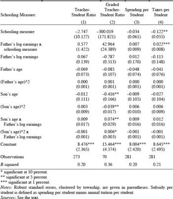
Appendix Tables 5 through 9 present the complete regression results for the estimates of intergenerational income elasticities conditional on school district quality. The coefficients for the interaction terms between father's log earnings and the schooling measure from these regressions are reported in Table 4 of the article. Each table corresponds to a different sample (urban, rural, rural outside of a town, rural inside of a town). It is important to note that in all tables son's age is defined as age minus 30. Therefore, coefficients on father's log earning and the interaction term between father's log earnings and the schooling measure give the intergenerational income elasticity for a 30-year-old son. Computing the income elasticity at any other age requires using all of the son's age—father's log earnings interaction coefficients as well.
INTERGENERATIONAL INCOME ELASTICITY ESTIMATES WITH SCHOOLING MEASURE INTERACTIONS FOR SONS FROM URBAN TOWNSHIPS, SON'S LOG EARNINGS AS DEPENDENT VARIABLE

* significant at 10 percent.
** significant at 5 percent.
*** significant at 1 percent.
Notes:
Standard errors, clustered by township, are given in parentheses. Graded schools dummy equals one if district has graded schools and zero otherwise. Subsidy per student is defined as spending per student minus annual tuition per student.
Sources:
See the text.
INTERGENERATIONAL INCOME ELASTICITY ESTIMATES WITH SCHOOLING MEASURE INTERACTIONS FOR SONS FROM RURAL TOWNSHIPS, SON'S LOG EARNINGS AS DEPENDENT VARIABLE

* significant at 10 percent.
** significant at 5 percent.
*** significant at 1 percent.
Notes:
Robust standard errors, clustered by township, are given in parentheses. Graded schools dummy equals one if district has graded schools and zero otherwise. Subsidy per student is defined as spending per student minus annual tuition per student.
Sources:
See the text.
INTERGENERATIONAL INCOME ELASTICITY ESTIMATES WITH SCHOOLING MEASURE INTERACTIONS FOR SONS FROM RURAL TOWNSHIPS LIVING OUTSIDE OF TOWNS, SON'S LOG EARNINGS AS DEPENDENT VARIABLE

Notes:
Robust standard errors, clustered by township, are given in parentheses. Subsidy per student is defined as spending per student minus annual tuition per student.
Sources:
See the text.
INTERGENERATIONAL INCOME ELASTICITY ESTIMATES WITH SCHOOLING MEASURE INTERACTIONS FOR SONS FROM RURAL TOWNSHIPS LIVING IN TOWNS (TOWNSHIP-LEVEL SCHOOL DATA), SON'S LOG EARNINGS AS DEPENDENT VARIABLE

* significant at 10 percent
** significant at 5 percent
*** significant at 1 percent
Notes:
Robust standard errors, clustered by township, are given in parentheses. Subsidy per student is defined as spending per student minus annual tuition per student.
Sources:
See the text.
INTERGENERATIONAL INCOME ELASTICITY ESTIMATES WITH SCHOOLING MEASURE INTERACTIONS FOR SONS FROM RURAL TOWNSHIPS LIVING IN TOWNS (TOWN LEVEL SCHOOL DATA), SON'S LOG EARNINGS AS DEPENDENT VARIABLE

* significant at 10 percent.
** significant at 5 percent.
*** significant at 1 percent.
Notes:
Robust standard errors, clustered by township, are given in parentheses. Subsidy per student is defined as spending per student minus annual tuition per student.
Sources:
See the text.
Appendix 2: Iowa Schools Data
The schooling data used throughout the article come from the Annual Reports of the Superintendent of Public Instruction. Each year, the superintendent of schools for each county in Iowa would submit a report to the superintendent of public instruction for the state. Included in this report was detailed information on the finances, enrollments, teachers, and miscellaneous details of the schools in the county.
AVAILABILITY OF TOWNSHIP AND DISTRICT-LEVEL DATA
Within a report for a single county, the information is broken down by either township or school district. For most rural townships, information is given for the township as a whole. The number of subdistricts in the township (typically corresponding to the number of common schools in the district) is listed but all of the data are reported for the township as a whole, not for each individual subdistrict. In some cases, data for each subdistrict was listed separately but this was rare.
In cases where there were independent towns or villages within a township, these towns or villages would have their own independent school district with its own information listed in the schools report. Consequently, for individuals living in rural counties, if they live in the open country the schools report would provide data at the township level while if they lived in a town, the schools report would provide data at the school district level.
These independent school districts typically contained the graded schools if a rural township had graded schools. Individuals living outside of the town had access to these schools, but typically had to pay an out-of-district tuition fee (the amount of which is given in the schools report). Given that a person living outside of a town with graded schools has different educational resources available to them than a person living outside of a town without graded schools, I combine the township school data with the data for the independent districts within a township to construct an overall measure of the educational resources in a township.
For urban counties (containing the cities of Davenport, Des Moines, and Dubuque), there are a large number of independent districts listed in the reports creating the possibility that individuals could be matched to their school districts. However, in these urban counties, the federal census records do not have sufficiently detailed location information to determine which school district an individual lives in (the location information given is typically the township name and then the name of the larger city). Consequently, it is necessary to aggregate these district data into township level data for the urban individuals.
VARIABLES REPORTED AT THE TOWNSHIP AND INDEPENDENT DISTRICT LEVEL
The information in the reports for the individual townships or independent districts is divided into several sections: schools, teachers and pupils, general, teachers' fund, schoolhouse fund, and contingent fund. Listed below are the items reported by section. Item names are given exactly as they are printed in the annual reports. The spending per student measures were calculated by summing all of the payments listed in the various fund sections. Taxes per student measures were calculated by summing the amounts received from district taxes in the various fund sections.
Schools—number ungraded, number rooms in the graded schools, and average number months taught.
Teachers and pupils — number employed males, number employed females, average compensation per month males, average compensation per month females, number of persons between the ages of 5 and 21 years males, number of persons between the ages of 5 and 21 years females, number enrolled in each district, total average attendance in the whole district, and average cost of tuition per month for each pupil.
General — number of schoolhouses, value of schoolhouses, value of apparatus, number of volumes in the libraries, number of trees in thrifty condition on the schoolhouse sites, and number of schoolrooms in which effects of stimulants and narcotics are taught.
Teachers' fund (debit section) — on hand last report, received from district tax, received from semiannual apportionment, received by transfer from schoolhouse fund, received from other sources.
Teachers' fund (credit section) — paid teachers since last report, paid other districts for tuition, paid for other purposes, on hand.
Schoolhouse fund (debit section) — on hand last report, received from district tax, received from other sources.
Schoolhouse fund (credit section) — paid for schoolhouses and sites, paid on bonds and interest, paid for library books, transferred to other funds, paid for other purposes, on hand.
Contingent fund (debit section) — on hand last report, received from district tax, received from sale of textbooks and supplies, received from schoolhouse fund and other sources.
Contingent fund (credit section) — Paid for fuel, rent, repairs, insurance and janitors, paid secretaries and treasurers, paid for records and apparatus, paid for library books and dictionaries, paid for free textbooks, paid for textbooks and general supplies, and paid for other purposes, on hand.
VARIABLES AVAILABLE AT THE COUNTY LEVEL
In addition to the information listed by township or independent district in the reports, there is a section of additional details given for the county as a whole. Included in this section is a listing of textbooks selected by the County Board of Education and the contract prices for those textbooks, responses to questions about the condition of country schools, reports of the examinations of teachers, statistics on the blind, deaf, dumb, and feeble-minded students, listings of colleges, academies, and private schools, and a report on the teachers' normal institute.
COVERAGE AND PUBLIC AVAILABILITY OF THE SCHOOLS DATA
These reports of the superintendents of schools were published annually and are available on microfilm from the Iowa State Historical Library. Scanned copies of the reports for the year 1900 are available for all Iowa counties from the author. Fully transcribed versions of the reports for the year 1900 for the counties used in this article will be made available for download.
Appendix 3: Mismatches and Mobility Estimation
The process of linking the 1915 Iowa census and 1900 federal census presents the possibility that some father-son pairs are incorrectly matched. Relying on name, age, and birthplace rather than a truly unique identifier makes the possibility of mismatches unavoidable. While every effort has been made to maintain strict criteria for matches, including discarding observations for which multiple individuals met the match criteria, the possibility of mismatches still looms. This section of the appendix offers a brief discussion of the estimation issues these mismatches create and an assessment of how common mismatches would have to be to account for the estimated difference in mobility rates between the 1915 Iowa and modern mobility estimates.
In its simplest incarnation, this mismatch error could be characterized as a son being paired with his correct father with probability π and incorrectly with a father drawn at random from the population with probability 1 - π. The value of the father's income used in the intergenerational income elasticity regressions is then given by

where yi, f is the father's true income, ui is a classical measurement error term, and ỹ is a randomly drawn income corresponding to some other father in the population. The distribution from which ỹ is drawn can be assumed to be the income distribution of the entire population. Alternatively, and perhaps more realistically, the income could come from a distribution of father's income conditional on the son's age. If the son and father are correctly matched, the income observation of the father will be his true income with some classical measurement error ui having mean zero and uncorrelated with the true income. The measurement error for the mismatched fathers will be equal to the difference between the randomly drawn income and his true income: ỹ - yi, f. Letting εi represent the measurement error for any given individual i in the sample and assuming that E(ỹ) is equal to E(yi, f), the measurement error for a sample containing some mismatched individuals can be characterized as follows,

This negative correlation between the measurement error and the true value of the father's income implies that the measurement error introduced by mismatching is mean reverting.
The problem of mean-reverting measurement error is not uncommon in the labor literature, especially in studies using various measures of income. Bonggeun Kim and Gary Solon outline the dramatic effects that mean-reverting measurement error can have on the economic interpretation of wage data.Footnote 2 Arie Kapteyn and Jelmer Ypman specifically consider the case of mismatched administrative income data and show that in the simple case where the mismeasured income variable is the single independent variable in a linear regression and mismatches are drawn from the same population as the correctly matched individuals, the estimated coefficient on income is biased downwards by an amount proportional to the rate of mismatches.Footnote 3
The bias introduced in the intergenerational income elasticity estimates by mismatched data is not easily characterized. The estimation equation includes both the mismatched variable and interactions of the mismatched variable with the correctly measured age of the son as regressors. Furthermore, the distribution from which a mismatch is drawn is dependent on the true value of the son's age. A final complication is that the likelihood of a son and father being mismatched may be correlated with characteristics of the son and father including age, income, location, literacy, and so on that enter the income elasticity regressions either directly or through the error term. All of these factors make it difficult to assess how large a problem mismatches are for the Iowa data. Unlike the classical measurement error for the income variables discussed in the article common to both the Iowa and modern data, this source of error is specific to the Iowa sample and consequently could lead to a bias that generates the observed difference in intergenerational income elasticities between the Iowa sample and modern data even if the true elasticities are the same.
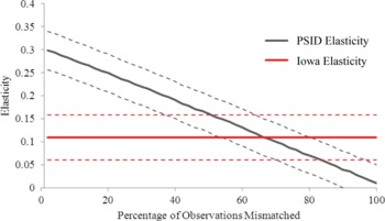
While there is no way to confidently state the number of mismatches in the linked Iowa sample, it is possible to introduce mismatches in a sample of observations from the Panel Study of Income Dynamics (PSID) and determine the level of mismatches required to obtain similar elasticity estimates for both the Iowa and PSID data. To generate random mismatches in the PSID data, an appropriate number of father-son observations are chosen at random to be mismatched. The father's income and age information is discarded. A new age for the father is randomly drawn from the distribution of father ages conditional on the son's age. The father's income is then randomly drawn from the distribution of income conditional on the father's newly chosen age. The new sample of individuals is then used to estimate the intergenerational income elasticity. The original data set is restored and then the entire process is repeated with new random number seeds.
Appendix Figure 1 depicts the results from simulating mismatches in the PSID sample. Mismatch rates of 2 percent to 100 percent are simulated, with 1,000 iterations of the mismatch and estimation procedure completed for each rate. The figure demonstrates that a mismatch rate approaching 50 percent would be required to account for the observed difference in 1915 and 2001 elasticities if the true elasticities are actually the same. Given that matches are identified by name, age, state of birth, father's state of birth, and mother's state of birth, the rate of mismatch in the linked Iowa data is likely far lower than this 50 percent figure.
INTERGENERATIONAL INCOME ELASTICITY ESTIMATES FOR THE 1915 IOWA SAMPLE AND THE 2001 PSID SAMPLE WITH RANDOM MISMATCHES IN THE PSID DATA