2 Numerical simulation

2.1 Problem formulation and numerical scheme

The simulation set-up and the numerical scheme in the present study are almost the same as those in Guo & Shen (Reference Guo and Shen2013). Here we shall provide only a brief description of the numerical method. For more details, readers should refer to Yang & Shen (Reference Yang and Shen2010) and Guo & Shen (Reference Guo and Shen2013).

Figure 1.

Simulation domain.

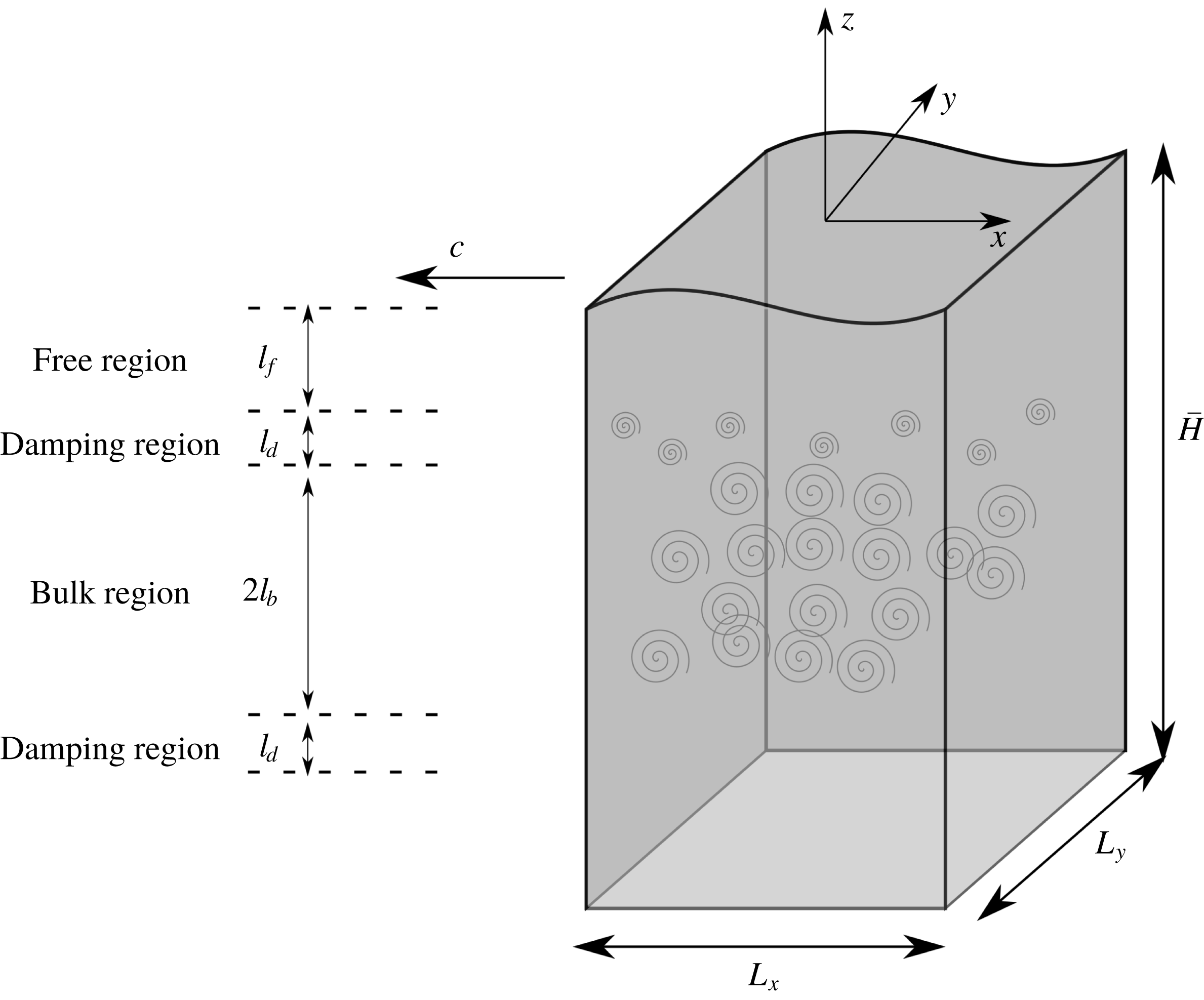
The computational domain is a cuboid at the beginning of the simulation, when the free surface is still and flat. A rectangular coordinate $(x,y,z)$ system is set up, with each coordinate axis parallel to an edge of the cuboid and the origin located at the centre of the top surface, as shown in figure 1. Homogeneous turbulence is generated in the bulk region of the domain by a body force $\boldsymbol{f}=A\boldsymbol{u}^{\prime }$ (Lundgren Reference Lundgren2003; Rosales & Meneveau Reference Rosales and Meneveau2005), where $\boldsymbol{u}^{\prime }$ is the difference between the local velocity $\boldsymbol{u}$ and its average over the $x{-}y$ plane. It is true that this turbulence generation method is not similar to some of the common sources of turbulence in the upper ocean layer, i.e. wave breaking and wind-induced shear current. However, the present turbulence generation method could still be relevant to some of the other mechanisms where the turbulence could be generated at some distance below the free surface, for example, turbulence driven by shear imposed by the ocean circulation or turbulence resulting from thermal convection. The amplitude coefficient $A$ is equal to a constant $A_{0}$ in the range of $-l_{b}<z-z_{c}\leqslant l_{b}$ , where $z_{c}$ is the vertical coordinate of the centre of the bulk region, and $l_{b}$ is half of the vertical length of the bulk region. In the damping region, $l_{b}<z-z_{c}\leqslant l_{b}+l_{d}$ , $A$ smoothly decays from $A_{0}$ to 0, where $l_{d}$ is the vertical length of the damping region. Above the damping region is the forcing-free region, $l_{b}+l_{d}<z-z_{c}\leqslant l_{b}+l_{d}+l_{f}$ , in which $A=0$ . Here $l_{f}$ is the vertical length of the forcing-free region satisfying $z_{c}+l_{b}+l_{d}+l_{f}=0$ . Below the bulk region, there are another damping region $-l_{b}-l_{d}<z-z_{c}\leqslant -l_{b}$ and another forcing-free region $z-z_{c}\leqslant -l_{b}-l_{d}$ . Hereafter, the free region only denotes the forcing-free region above the bulk region.

At the surface, a progressive wave is generated and maintained by the method proposed by Guo & Shen (Reference Guo and Shen2009). A feedback control system is constructed in the method. At each time step, the difference between the surface elevation $\unicode[STIX]{x1D702}(x,y,t)$ and the elevation $\unicode[STIX]{x1D6E4}(x,y,t)$ of a target progressive wave is monitored. An additional pressure distribution $p_{a}(x,y,t)$ is applied at the free surface to eliminate the elevation difference; and $p_{a}(x,y,t)$ is obtained by solving a linearized Cauchy–Poisson problem which gives the relationship between $p_{a}(x,y,t)$ and the response of $\unicode[STIX]{x1D702}(x,y,t)$ . After several wave periods, $\unicode[STIX]{x1D702}(x,y,t)$ is very close to $\unicode[STIX]{x1D6E4}(x,y,t)$ , and $p_{a}(x,y,t)$ decays eventually to a negligible level.

The streamwise direction (i.e. the direction that is aligned with the direction of wave propagation), the spanwise direction and the vertical direction are denoted as $x$ , $y$ and $z$ (also written as $x_{1},x_{2},x_{3}$ ), respectively. The flow is governed by the incompressible Navier–Stokes equations

(2.1) $$\begin{eqnarray}\frac{\unicode[STIX]{x2202}u_{i}}{\unicode[STIX]{x2202}t}+\frac{\unicode[STIX]{x2202}u_{i}u_{j}}{\unicode[STIX]{x2202}x_{j}}=-\frac{1}{\unicode[STIX]{x1D70C}}\frac{\unicode[STIX]{x2202}p}{\unicode[STIX]{x2202}x_{i}}+\unicode[STIX]{x1D708}\frac{\unicode[STIX]{x2202}^{2}u_{i}}{\unicode[STIX]{x2202}x_{j}\unicode[STIX]{x2202}x_{j}}-g\unicode[STIX]{x1D6FF}_{i3}+Au_{i}^{\prime },\end{eqnarray}$$

and the continuity equation

(2.2) $$\begin{eqnarray}\frac{\unicode[STIX]{x2202}u_{i}}{\unicode[STIX]{x2202}x_{i}}=0,\end{eqnarray}$$

where $\unicode[STIX]{x1D70C}$ is the density, $p$ is the pressure, $g$ is the gravitational acceleration, $\unicode[STIX]{x1D6FF}_{ij}$ is the Kronecker delta and $\unicode[STIX]{x1D708}$ is the kinematic viscosity. Surface elevation $\unicode[STIX]{x1D702}$ is governed by the kinematic boundary condition at the free surface:

(2.3) $$\begin{eqnarray}\frac{\unicode[STIX]{x2202}\unicode[STIX]{x1D702}}{\unicode[STIX]{x2202}t}+u\frac{\unicode[STIX]{x2202}\unicode[STIX]{x1D702}}{\unicode[STIX]{x2202}x}+v\frac{\unicode[STIX]{x2202}\unicode[STIX]{x1D702}}{\unicode[STIX]{x2202}y}-w=0.\end{eqnarray}$$

The tangential stresses at the free surface are forced to be zero. The normal stress is equal to the constant atmospheric pressure $p_{0}$ . At the bottom of the domain at $z=-H$ , where $H$ is the height of the domain when the free surface is still, a free-slip boundary condition is applied. In the two horizontal directions, periodic boundary conditions are used.

Owing to the propagation of the surface wave, the shape of the simulation domain changes over time. To keep the computational grid invariant in time, a mapping from the Cartesian system $(x,y,z,t)$ to the curvilinear system $(\unicode[STIX]{x1D709},\unicode[STIX]{x1D713},\unicode[STIX]{x1D701},\unicode[STIX]{x1D704})$ is introduced:

(2.4) $$\begin{eqnarray}\left.\begin{array}{@{}c@{}}\displaystyle \unicode[STIX]{x1D709}=x,\\ \displaystyle \unicode[STIX]{x1D713}=y,\\ \displaystyle \unicode[STIX]{x1D701}=\frac{z+H}{\unicode[STIX]{x1D702}+H},\\ \displaystyle \unicode[STIX]{x1D704}=t.\end{array}\right\}\end{eqnarray}$$

By the chain rule, we obtain the following relations:

(2.5) $$\begin{eqnarray}\left.\begin{array}{@{}c@{}}\displaystyle \frac{\unicode[STIX]{x2202}}{\unicode[STIX]{x2202}x}=\frac{\unicode[STIX]{x2202}}{\unicode[STIX]{x2202}\unicode[STIX]{x1D709}}-\frac{\unicode[STIX]{x1D701}\unicode[STIX]{x1D702}_{x}}{\unicode[STIX]{x1D702}+H}\frac{\unicode[STIX]{x2202}}{\unicode[STIX]{x2202}\unicode[STIX]{x1D701}},\\ \displaystyle \frac{\unicode[STIX]{x2202}}{\unicode[STIX]{x2202}y}=\frac{\unicode[STIX]{x2202}}{\unicode[STIX]{x2202}\unicode[STIX]{x1D713}}-\frac{\unicode[STIX]{x1D701}\unicode[STIX]{x1D702}_{y}}{\unicode[STIX]{x1D702}+H}\frac{\unicode[STIX]{x2202}}{\unicode[STIX]{x2202}\unicode[STIX]{x1D701}},\\ \displaystyle \frac{\unicode[STIX]{x2202}}{\unicode[STIX]{x2202}z}=\frac{1}{\unicode[STIX]{x1D702}+H}\frac{\unicode[STIX]{x2202}}{\unicode[STIX]{x2202}\unicode[STIX]{x1D701}},\\ \displaystyle \frac{\unicode[STIX]{x2202}}{\unicode[STIX]{x2202}t}=\frac{\unicode[STIX]{x2202}}{\unicode[STIX]{x2202}\unicode[STIX]{x1D704}}-\frac{\unicode[STIX]{x1D701}\unicode[STIX]{x1D702}_{t}}{\unicode[STIX]{x1D702}+H}\frac{\unicode[STIX]{x2202}}{\unicode[STIX]{x2202}\unicode[STIX]{x1D701}}.\end{array}\right\}\end{eqnarray}$$

The governing equations (2.1), (2.2) and (2.3) together with the boundary conditions are rewritten and solved in the curvilinear space $(\unicode[STIX]{x1D709},\unicode[STIX]{x1D713},\unicode[STIX]{x1D701},\unicode[STIX]{x1D704})$ .

Three differences exist between the scheme in the present study and that of Yang & Shen (Reference Yang and Shen2010) and Guo & Shen (Reference Guo and Shen2013). First, in the $\unicode[STIX]{x1D701}$ direction, a fourth-order compact finite-difference scheme is employed here, which produces a better approximation of $\unicode[STIX]{x2202}^{2}/\unicode[STIX]{x2202}\unicode[STIX]{x1D701}^{2}$ and better balance of the budget equation for the turbulent energy, such as the balance in (4.2) in this paper. Yang & Shen (Reference Yang and Shen2010) and Guo & Shen (Reference Guo and Shen2013) used a second-order central-difference scheme, which seems to inaccurately represent the dissipation in the $\unicode[STIX]{x1D701}$ direction. Second, the wave is propagating in the $-x$ direction in this study. The last difference is that the vertical domain size here is $6\unicode[STIX]{x03C0}$ rather than $5\unicode[STIX]{x03C0}$ , aiming to reduce the effect of the bottom boundary on the bulk region and the free region. Nevertheless, the difference introduced by using a larger domain depth is negligible.

2.2 Computational parameters

We assume the horizontal domain size is set to $2\unicode[STIX]{x03C0}L$ , and $L$ is used as the physical length scale. The characteristic velocity scale $U$ is set to $10LA_{0}$ . Hereafter, if not explicitly declared, variables are non-dimensionalized by $U$ and $L$ . The dimensionless domain size is $L_{x}\times L_{y}\times L_{z}=2\unicode[STIX]{x03C0}\times 2\unicode[STIX]{x03C0}\times 6\unicode[STIX]{x03C0}$ . In the vertical direction, the dimensionless subdomain scales are $l_{b}=3\unicode[STIX]{x03C0}/2,~l_{d}=\unicode[STIX]{x03C0}/2$ and $l_{f}=\unicode[STIX]{x03C0}/2$ . The surface wave has the dimensionless wavenumber $k_{W}$ and dimensionless amplitude $a$ , from which the wave steepness is defined as $Stp=ak_{W}$ . The Reynolds number is defined as $Re=UL/\unicode[STIX]{x1D708}$ and the Froude number is $Fr=U/\sqrt{gL}$ . In all simulations, $k_{W}=1$ , which means the streamwise direction contains just one wavelength.

The linear deep-water wave theory (Lighthill Reference Lighthill1978) shows that the wave-induced motion decays exponentially as $\exp (-k_{W}|z|)$ , where $|z|$ is the distance to the initially still free surface. Thus the ratio of the wave straining in the bulk region to that near the free surface is approximately $\exp [-k_{W}(l_{f}+l_{d})]=0.043$ , which is negligible; while the ratio of the wave straining in the free region to that near the free surface is around $\exp (-k_{W}l_{f}/2)=0.456$ . In accordance with Guo & Shen (Reference Guo and Shen2013, Reference Guo and Shen2014), the turbulent statistics at $z^{cf}=-l_{f}/2$ , when the surface wave has not been enforced, are used to normalize the statistics in the free region. The superscript ‘ $cf$ ’ denotes the centre of the free region. Some important statistics are the root mean square (r.m.s.) of the turbulent velocity $u^{rms,cf}$ , the Taylor scale $\unicode[STIX]{x1D706}^{cf}$ , the integral length scale $L_{\infty }^{cf}$ , the turbulence kinetic energy $q^{cf}$ and the turbulence dissipation rate $\unicode[STIX]{x1D716}^{cf}$ . The Taylor-scale Reynolds number is defined as $Re_{\unicode[STIX]{x1D706}}^{cf}=u^{rms,cf}\unicode[STIX]{x1D706}^{cf}/\unicode[STIX]{x1D708}$ . The wave-induced straining intensity is characterized by $S=ak_{W}\unicode[STIX]{x1D714}$ , where $\unicode[STIX]{x1D714}=\sqrt{k_{W}}/Fr$ is the wave circular frequency. Hence the wave straining to turbulence straining ratio is $Sq^{cf}/\unicode[STIX]{x1D716}^{cf}$ , and the turbulence integral length to wavelength ratio is $L_{\infty }^{cf}/\unicode[STIX]{x1D6EC}$ , where $\unicode[STIX]{x1D6EC}=2\unicode[STIX]{x03C0}$ is the wavelength. In the present study, the turbulence integral length to wavelength ratio is quite small ( $L_{\infty }^{cf}/\unicode[STIX]{x1D6EC}\ll 1$ ) and the wave straining to turbulence straining ratio is very large ( $Sq^{cf}/\unicode[STIX]{x1D716}^{cf}\gg 1$ ).

Such a configuration of turbulence and wave is chosen not only because it has been discussed in previous literature (Teixeira & Belcher Reference Teixeira and Belcher2002; Guo & Shen Reference Guo and Shen2013, Reference Guo and Shen2014), but also because it is a reasonable simplification of a number of experimental studies and oceanic observations. The integral length scale of turbulence in a grid stirred tank (Brumley & Jirka Reference Brumley and Jirka1987) or associated with wave-induced current (Melville et al. Reference Melville, Shear and Veron1998) is $O(1~\text{cm})$ or larger. Turbulence generated by a breaking wave has a larger integral length scale, ranging from $O(10~\text{cm})$ to $O(1~\text{m})$ (Kitaigorodskii & Lumley Reference Kitaigorodskii and Lumley1983; Rapp & Melville Reference Rapp and Melville1990). As a comparison, the wavelength corresponding to the peak of the wave-height spectrum is $O(10~\text{m})$ in a lake (Kitaigorodskii & Lumley Reference Kitaigorodskii and Lumley1983) and $O(100~\text{m})$ in the ocean (Forristall Reference Forristall1981; He, Howell & Walsh Reference He, Howell and Walsh1993), which is much larger than the integral length scale of the turbulence. The ratio of wave straining to turbulence straining at peak wavenumber $k_{p}$ calculated with data from Kitaigorodskii & Lumley (Reference Kitaigorodskii and Lumley1983) is around $4$ . For waves with wavenumber larger than $k_{p}$ , the straining ratio can greatly exceed  $4$ . Therefore, it is acceptable to assume wave straining much stronger than turbulent straining.

Table 1.

The computational parameters in the simulations.

Table 2.

The turbulent characteristics at the centre of the free region.

Figure 2.

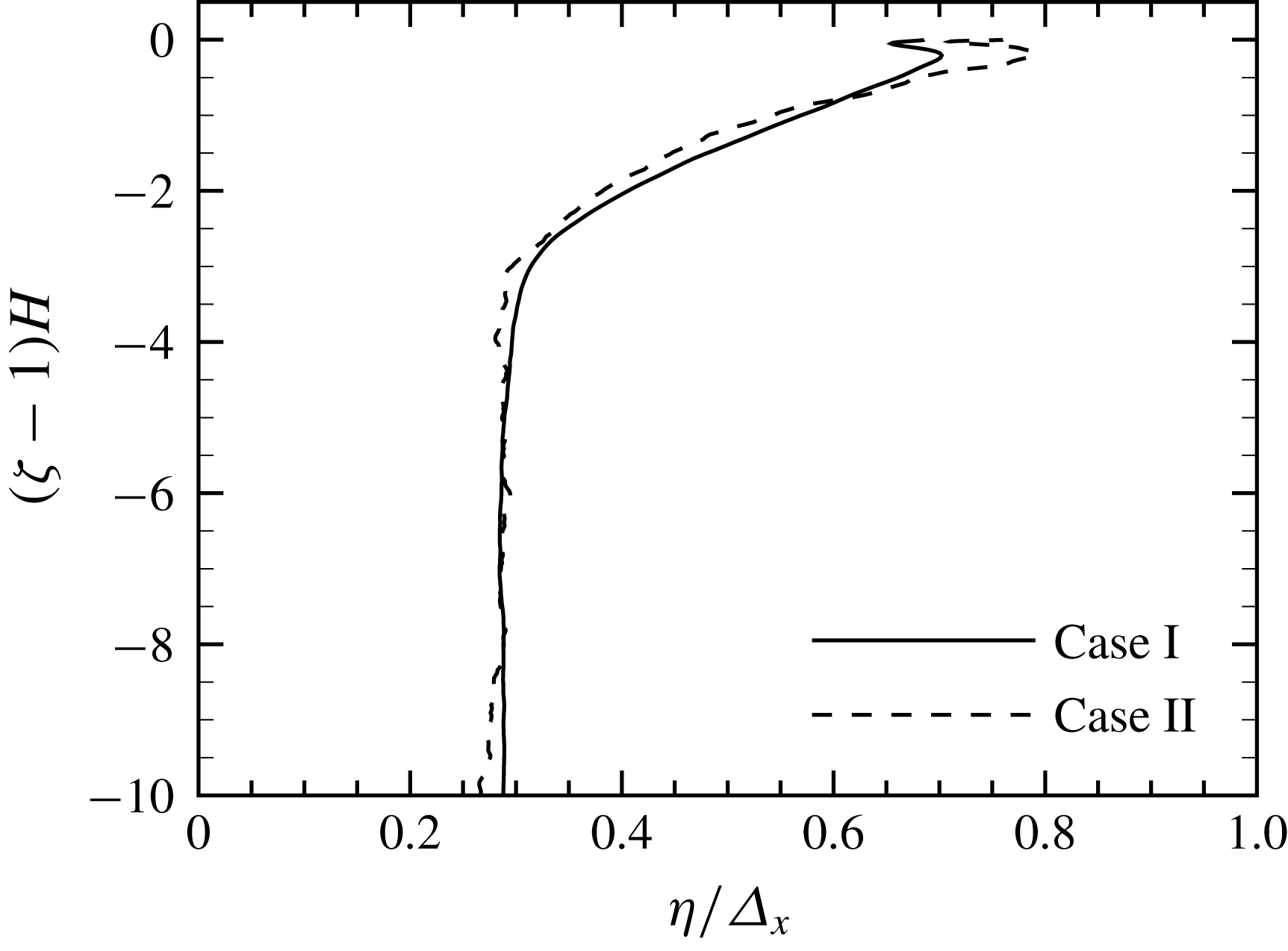
The variation of the Kolmogorov scale when a surface wave is not enforced, normalized by the grid spacing in the horizontal directions: solid line for case I; dashed line for case II.

The free-surface simulation requires much more computing resource compared to a traditional turbulent channel-flow simulation. As a result, the mesh size and Reynolds number are considerably limited. In case I, the mesh size is $N_{x}\times N_{y}\times N_{z}=128\times 128\times 348$ . The local grid spacing in horizontal directions is $\unicode[STIX]{x1D6E5}_{x}=\unicode[STIX]{x1D6E5}_{y}=0.0491$ . The maximum local grid spacing in the vertical direction is $\unicode[STIX]{x1D6E5}_{z,max}=0.0575$ within the bulk region, and the minimum local grid spacing is $\unicode[STIX]{x1D6E5}_{z,min}=0.00287$ at the free surface. To achieve a larger Reynolds number, case II is performed with mesh size $N_{x}\times N_{y}\times N_{z}=256\times 256\times 600$ . The local grid spacing becomes $\unicode[STIX]{x1D6E5}_{x}=\unicode[STIX]{x1D6E5}_{y}=0.0245$ , $\unicode[STIX]{x1D6E5}_{z,max}=0.0330$ and $\unicode[STIX]{x1D6E5}_{z,min}=6.60\times 10^{-4}$ . The computational parameters are listed in table 1. The turbulent characteristics at the centre of the free region are listed in table 2. When the surface wave is not enforced, the variation of the Kolmogorov scales from the bulk region to the free surface is displayed in figure 2. Above the damping region, the turbulence strength is weaker and the dissipation rate $\unicode[STIX]{x1D716}$ becomes smaller with decreasing distance from the free surface. As a result, the Kolmogorov scales $\unicode[STIX]{x1D702}\sim (\unicode[STIX]{x1D708}^{3}/\unicode[STIX]{x1D716})^{1/4}$ increase when approaching the free surface. In the bulk region the Kolmogorov scales are almost constant with $\unicode[STIX]{x1D702}/\unicode[STIX]{x1D6E5}_{x}\approx 0.38$ . The ratio is less than $0.48$ , the criterion for resolving the smallest turbulence motion (see Pope Reference Pope2000). Nevertheless, $\unicode[STIX]{x1D702}/\unicode[STIX]{x1D6E5}_{x}\approx 0.55$ at the centre of the free region. Thus the grid solution is sufficient at least in the free region, which is the region of interest in the present study.

3 Subgrid-scale stress and energy flux

We now introduce the average operators that will be used later: $\langle \cdot \rangle$ represents the wave phase average; $(\cdot )_{WH}$ represents a Lagrangian average when a wave particle travels one wavelength in the reference frame fixed on the surface wave. The wave particle here is the particle convected by the wave-induced velocity. 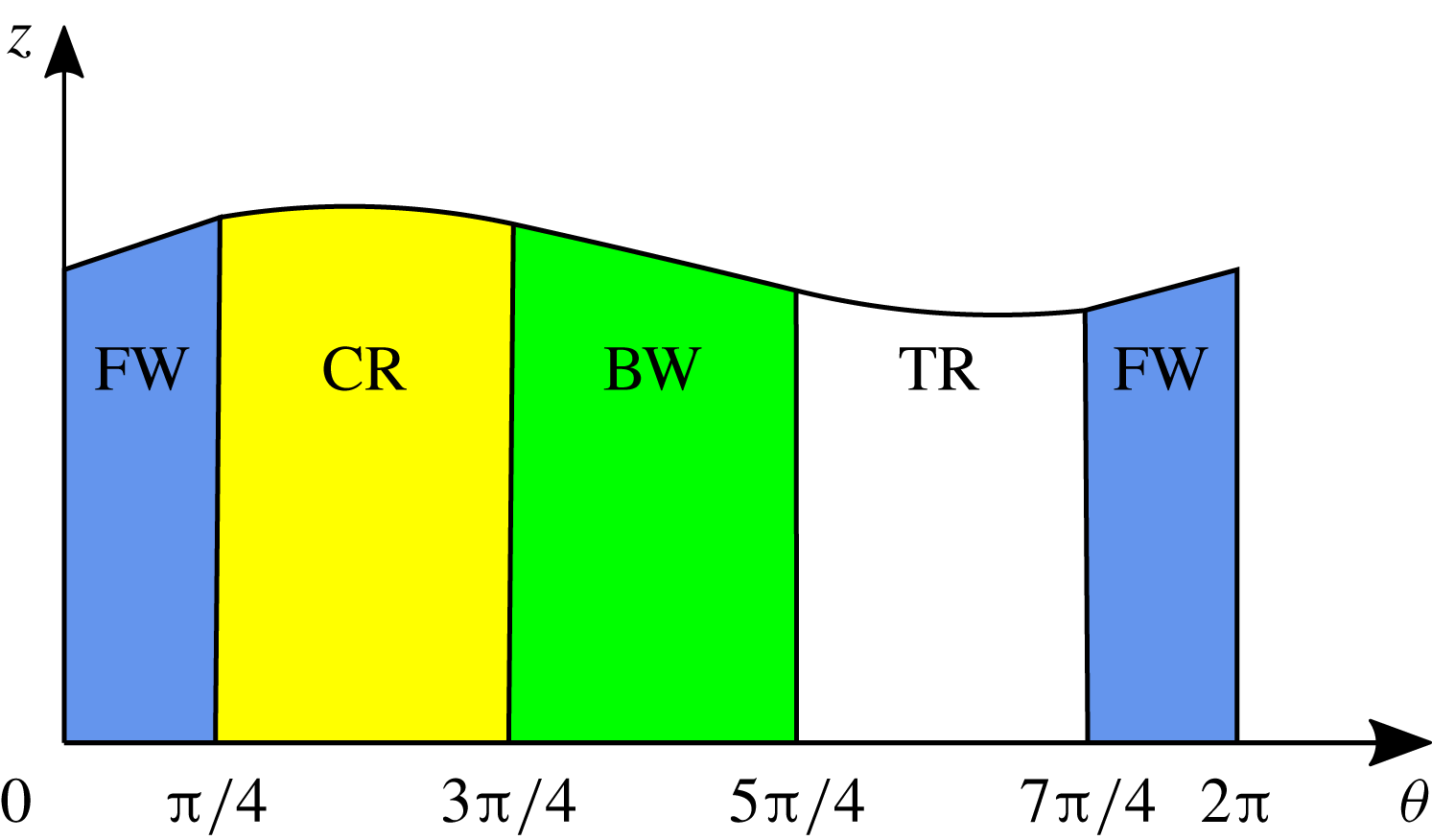Operators $(\cdot )_{FW}$ , $(\cdot )_{CR}$ , $(\cdot )_{BW}$ and $(\cdot )_{TR}$ denote the Lagrangian average when the wave particle passes through four wave shape ranges, i.e. the forward slope range, the crest range, the backward slope range and the trough range, respectively. Figure 3 is a sketch of the four wave shape ranges. These average operators’ mathematical definitions can be found in appendix A.

Figure 3.

Four wave shape ranges: the forward slope range is blue, the crest range is yellow, the backward slope range is green and the trough range is white.

The SGS stress is defined as

(3.1) $$\begin{eqnarray}\unicode[STIX]{x1D70F}_{ij}=\widetilde{u_{i}u_{j}}-\tilde{u} _{i}\tilde{u} _{j}.\end{eqnarray}$$

Here $\widetilde{(\cdot )}$ represents a two-dimensional (2-D) Gaussian filter in the $\unicode[STIX]{x1D709}{-}\unicode[STIX]{x1D713}$ plane, which is defined in (A 12) in appendix A. A three-dimensional (3-D) Gaussian filter in the curvilinear coordinate system, a 3-D Gaussian filter in the Cartesian coordinate system and a 2-D spectral cutoff filter are also considered and the results are quite similar to those of the 2-D Gaussian filter, thus are not shown. Following Guo & Shen (Reference Guo and Shen2013, Reference Guo and Shen2014) the velocity field is decomposed into the wave-induced motion and the turbulent motion:

(3.2) $$\begin{eqnarray}u_{i}=u_{i}^{W}+u_{i}^{T}.\end{eqnarray}$$

The wave-induced motion is obtained by $u_{i}^{W}=\langle u_{i}\rangle$ . Substituting the decomposition in (3.2) for the velocity in (3.1), the SGS stress is decomposed into three parts:

(3.3) $$\begin{eqnarray}\unicode[STIX]{x1D70F}_{ij}=\unicode[STIX]{x1D70F}_{ij}^{T}+\unicode[STIX]{x1D70F}_{ij}^{C}+\unicode[STIX]{x1D70F}_{ij}^{W},\end{eqnarray}$$

where

(3.4) $$\begin{eqnarray}\unicode[STIX]{x1D70F}_{ij}^{T}=\widetilde{u_{i}^{T}u_{j}^{T}}-\widetilde{u_{i}^{T}}\widetilde{u_{j}^{T}}\end{eqnarray}$$

is the turbulent SGS stress,

(3.5) $$\begin{eqnarray}\unicode[STIX]{x1D70F}_{ij}^{C}=\widetilde{u_{i}^{T}u_{j}^{W}}-\widetilde{u_{i}^{T}}\widetilde{u_{j}^{W}}+\widetilde{u_{i}^{W}u_{j}^{T}}-\widetilde{u_{i}^{W}}\widetilde{u_{j}^{T}}\end{eqnarray}$$

is the cross-interaction stress, and the third part

(3.6) $$\begin{eqnarray}\unicode[STIX]{x1D70F}_{ij}^{W}=\widetilde{u_{i}^{W}u_{j}^{W}}-\widetilde{u_{i}^{W}}\widetilde{u_{j}^{W}}\end{eqnarray}$$

is the wave-induced stress. This decomposition was first proposed in Liu et al. (Reference Liu, Katz and Meneveau1999).

Figure 4.

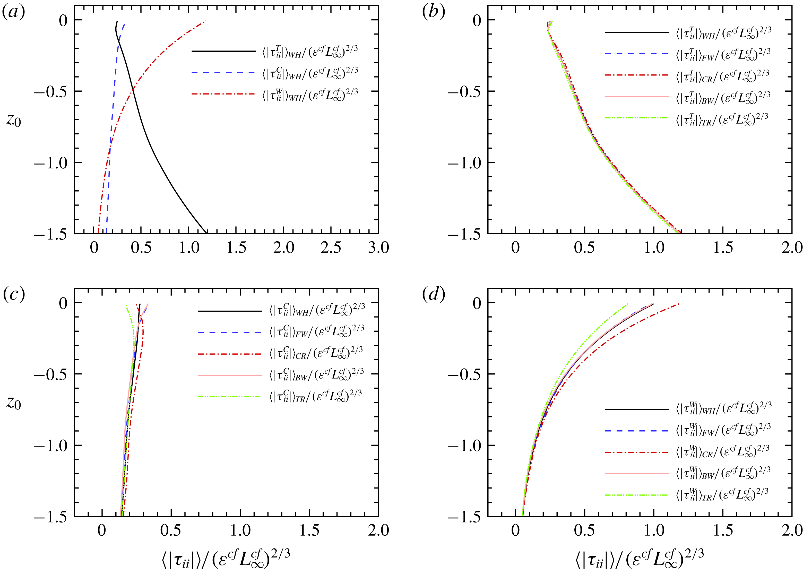
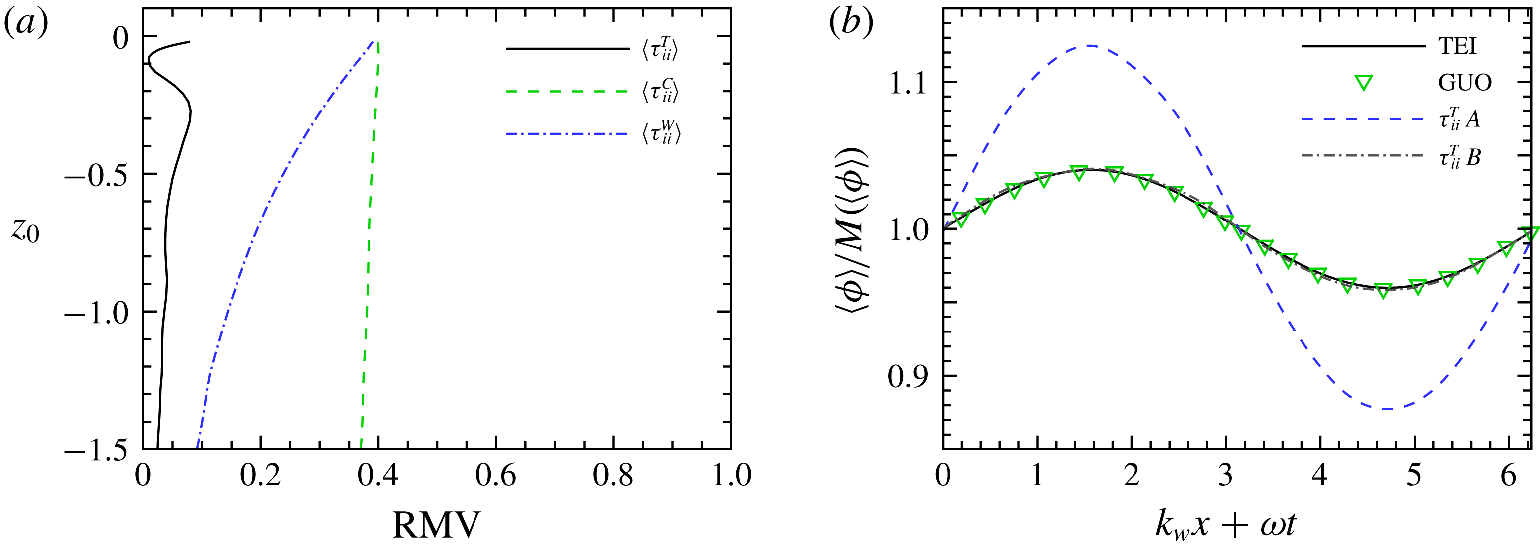
From case I: (a) magnitude of different SGS stress terms along the depth; (b) magnitude of $\unicode[STIX]{x1D70F}_{ii}^{T}$ in different wave shape ranges; (c) magnitude of $\unicode[STIX]{x1D70F}_{ii}^{C}$ in different wave shape ranges; and (d) magnitude of $\unicode[STIX]{x1D70F}_{ii}^{W}$ in different wave shape ranges.

Figure 4 shows the values of the different SGS stress terms along the vertical direction and its wave shape range dependence in case I. The repeated indices in figure 4 and in the rest of this study imply summation, as in the Einstein summation convention. Throughout the paper, if not specified, $z_{0}$ is the initial vertical position of the wave particle based on which the wave shape range average operators are defined (see appendix A). The filter width $\unicode[STIX]{x1D6E5}_{c}=0.46L_{\infty }^{cf}=0.05\unicode[STIX]{x1D6EC}$ . Though the filter width is quite large compared to that in many other LES studies, the curves of the SGS stresses versus depth are found to have similar trends in the filter width range of $0.11L_{\infty }^{cf}<\unicode[STIX]{x1D6E5}_{c}\leqslant 0.46L_{\infty }^{cf}$ . In figure 4(a), $\unicode[STIX]{x1D70F}_{ii}^{T}$ has its minimum at the free surface and increases with increasing depth, because the turbulence is generated in the bulk region and decays with distance from the bulk region. Meanwhile, $\unicode[STIX]{x1D70F}_{ii}^{W}$ decreases with increasing depth, consistent with the exponential decay of the linear deep-water wave. The $\unicode[STIX]{x1D70F}_{ii}^{C}$ value also decreases but much slower than $\unicode[STIX]{x1D70F}_{ii}^{W}$ . Note that for two reasons no conclusion about the relative magnitudes among the different SGS stress terms can be drawn from figure 4. First, their magnitudes change with the filter width at different rates. Second, $Sq^{cf}/\unicode[STIX]{x1D716}^{cf}$ has a direct influence on the ratio of their magnitudes (see (3.18)). From figure 4(b), $\unicode[STIX]{x1D70F}_{ii}^{T}$ has almost the same averaged magnitude at different wave shape ranges in the free region, within which the wave straining is prominent. As expected, the curves of $\unicode[STIX]{x1D70F}_{ii}^{W}$ in different wave shape ranges and those of $\unicode[STIX]{x1D70F}_{ii}^{C}$ diverge greatly when the depth decreases (see figure 4 c,d).

Figure 5.

From case I: (a) relative variance of $\langle \unicode[STIX]{x1D70F}_{ii}^{T}\rangle$ , $\langle \unicode[STIX]{x1D70F}_{ii}^{C}\rangle$ and $\langle \unicode[STIX]{x1D70F}_{ii}^{W}\rangle$ along the trajectories of wave particles released at different depths; and (b) other RVs, where $M(\langle \unicode[STIX]{x1D719}\rangle )$ is the mean value of $\langle \unicode[STIX]{x1D719}\rangle$ , TEI is $\langle (u_{1}^{T})^{2}\rangle$ based on Teixeira & Belcher (Reference Teixeira and Belcher2002) (see (3.7)) at $z=-0.69$ , GUO is $\langle (u_{1}^{T})^{2}\rangle$ at $z=-0.69$ extracted from figure 2(a) of Guo & Shen (Reference Guo and Shen2014), $\unicode[STIX]{x1D70F}_{11}^{T}$  A is $\langle \unicode[STIX]{x1D70F}_{11}^{T}\rangle$ at $z=-0.69$ , and $\unicode[STIX]{x1D70F}_{11}^{T}$  B is $\langle \unicode[STIX]{x1D70F}_{11}^{T}\rangle$ along the trajectories of a wave particle released at $x=0,~z=-0.69$ .

Now we analyse the actual variation of the SGS stress with different phases, which is very likely reduced by the wave shape range average operators. Furthermore, the phase dependence of a variable is better explained by relative variation than by absolute variation. The relative variation (RV) of a variable $\unicode[STIX]{x1D719}$ along a line is conveniently defined as $\unicode[STIX]{x1D719}$ divided by its mean value along the same line. The relative maximum variation (RMV) is then defined as the difference between the maximum and the minimum of RV. The RMV of $\langle \unicode[STIX]{x1D70F}_{ii}^{T}\rangle$ along the trajectories of wave particles released at different depths involved in figure 5(a) is found to be no more than $8\,\%$ , while those of $\langle \unicode[STIX]{x1D70F}_{ii}^{C}\rangle$ and $\langle \unicode[STIX]{x1D70F}_{ii}^{W}\rangle$ can reach $40\,\%$ . So it is reasonable to state that the turbulent SGS stress has the least phase dependence among the three parts of the SGS stress.

When measuring variation with phase by RV, the trajectory along which RV is evaluated influences the results. A line with constant depth has been utilized in several experiments (Jiang & Street Reference Jiang and Street1991; Thais & Magnaudet Reference Thais and Magnaudet1996) and simulations (Komori et al. Reference Komori, Kursose, Iwano, Ukai and Naoya2010; Guo & Shen Reference Guo and Shen2014), while a wave particle trajectory is adopted in Teixeira & Belcher (Reference Teixeira and Belcher2002). The line $\unicode[STIX]{x1D70F}_{11}^{T}$  B in figure 5(b) plots the RV of $\langle \unicode[STIX]{x1D70F}_{11}^{T}\rangle$ along the trajectory of a wave particle released at $x=0,~z=-0.47$ , and the line $\unicode[STIX]{x1D70F}_{11}^{T}$  A shows the RV at a constant depth $z=-0.47$ , whose RMV is at least three times that of $\unicode[STIX]{x1D70F}_{11}^{T}$  B. One possible explanation for the larger RMV in line $\unicode[STIX]{x1D70F}_{11}^{T}$  A is that wave particles in the straight line with a constant depth have experienced different histories along different trajectories, which amplifies their difference. For example, the wave particle that passes through the point beneath the crest and at $z=-0.69$ is released at $x=0,~z=-0.53$ and the wave particle that passes through the point beneath the trough and at $z=-0.69$ is released at $x=0,~z=-0.41$ . It is found that $\langle \unicode[STIX]{x1D70F}_{11}^{T}\rangle _{WH}$ for the former wave particle is larger than $\langle \unicode[STIX]{x1D70F}_{11}^{T}\rangle _{WH}$ for the latter wave particle and their difference is approximately $21\,\%$ of $\langle \unicode[STIX]{x1D70F}_{11}^{T}\rangle _{WH}$ for the wave particle released at $x=0,~z=-0.69$ . This percentage is more than two times the RMV of $\unicode[STIX]{x1D70F}_{11}^{T}$  B, which approximately explains the difference between the RMV of $\unicode[STIX]{x1D70F}_{11}^{T}$  A and that of $\unicode[STIX]{x1D70F}_{11}^{T}$  B.

The variation of streamwise-normal component of Reynolds stress $\langle (u_{1}^{T})^{2}\rangle$ is also shown in figure 5(b) for comparison; $\langle (u_{1}^{T})^{2}\rangle$ is the contribution to the turbulent kinetic energy from the streamwise turbulent motion at all scales. And $\langle \unicode[STIX]{x1D70F}_{11}^{T}\rangle$ could be regarded as the contribution of the streamwise SGS turbulent motion to the SGS kinetic energy. Equation (3.8) in Teixeira & Belcher (Reference Teixeira and Belcher2002), which results from an approximation where the off-diagonal components of the strain tensor associated with the wave motion are neglected, is rewritten here considering that the phase is determined according to the surface shape $\unicode[STIX]{x1D702}=a\sin (k_{W}x+\unicode[STIX]{x1D714}t)$ :

(3.7) $$\begin{eqnarray}\frac{\langle (u_{1}^{T})^{2}\rangle }{(u_{in}^{rms})^{2}}=1+\frac{4}{5}ak_{W}\exp (k_{W}z)\sin (k_{W}x+\unicode[STIX]{x1D714}t),\end{eqnarray}$$

where $u_{in}^{rms}$ is the r.m.s. value of the turbulent velocity at the initial position of a wave particle. Equation (3.7) gives a good estimation of the RV of $\langle (u_{1}^{T})^{2}\rangle$ along a wave particle trajectory. When the initial position of the wave particle is $x=0,~z=-0.69$ , equation (3.7) is drawn as line TEI in figure 5(b). Obviously, line $\unicode[STIX]{x1D70F}_{11}^{T}$  B is close to line TEI, indicating that the relative variation of the SGS turbulent motion is similar to that of the turbulent motion of all scales. The numerical result of Guo & Shen (Reference Guo and Shen2014) (figure 2a in their paper) at the fixed depth is shown as symbols GUO. Although line $\unicode[STIX]{x1D70F}_{11}^{T}$  A and symbols GUO are gathered at the same depth, the variation in line $\unicode[STIX]{x1D70F}_{11}^{T}$  A is much larger than that in the latter one. We have compared the contour lines of $\langle \unicode[STIX]{x1D70F}_{11}^{T}\rangle$ with figure 3(a) of Guo & Shen (Reference Guo and Shen2014), which shows the contour lines of $\langle (u_{1}^{T})^{2}\rangle$ . It is found that if the distance to the free surface is fixed at $0.69$ , values of $\langle \unicode[STIX]{x1D70F}_{11}^{T}\rangle$ at different phases are more concentrated than those of $\langle (u_{1}^{T})^{2}\rangle$ . Consequently, at the constant depth, the RMV of $\langle \unicode[STIX]{x1D70F}_{11}^{T}\rangle$ is much larger than that of $\langle (u_{1}^{T})^{2}\rangle$ .

Figure 6.

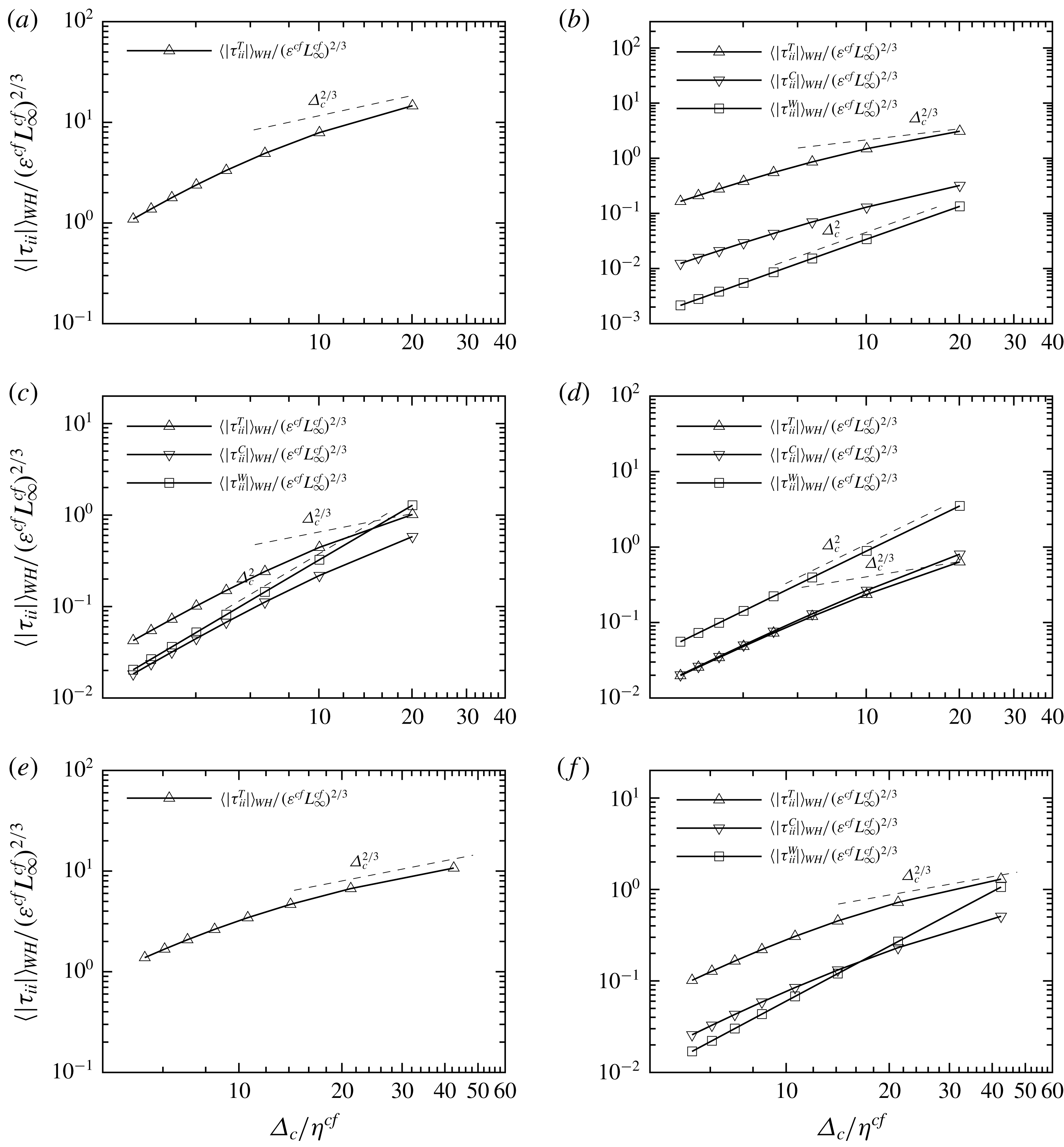
Scale dependence of the magnitude of different SGS stress terms at different depth: (a)  $z_{0}=-7.4$ , from case I; (b)  $z_{0}=-1.7$ , from case I; (c)  $z_{0}=-0.6$ , from case I; (d)  $z_{0}=-0.06$ , from case I; (e)  $z_{0}=-7.4$ , from case II; and (f)  $z_{0}=-0.6$ , from case II.

The effect of the filter width on the magnitudes of the SGS stress terms is plotted in figure 6. Figure 6(a–d) show results at several locations in case I. Figure 6(e,f) are extracted from two locations in case II. The magnitudes of $\unicode[STIX]{x1D70F}_{ii}^{C}$ and $\unicode[STIX]{x1D70F}_{ii}^{W}$ are negligible in the bulk region, hence are not drawn in figure 6(a). In the inertial range, the Kolmogorov scaling for isotropic turbulence yields a scaling of the SGS stress as $|\unicode[STIX]{x1D70F}|\sim {\unicode[STIX]{x1D6E5}_{c}}^{2/3}$ . Owing to the shortness of the inertial range, the actual scaling of $\langle |\unicode[STIX]{x1D70F}_{ii}^{T}|\rangle$ can only be roughly determined by the slope of the straight line connecting the two data points at the two largest filter widths. Among the three different SGS stress terms, the scaling of $\langle |\unicode[STIX]{x1D70F}_{ii}^{T}|\rangle$ is closest to the Kolmogorov scaling, but still steeper than the latter. Many factors could affect this scaling, for example, the Reynolds number, the wave straining and the forcing scheme used to maintain the turbulence.

In the results from case I at $z_{0}=-7.4$ , where local $Re_{\unicode[STIX]{x1D706}}=67.2$ , the wave straining is negligible and only a very limited inertial range emerges (see figure 6 a) due to the small $Re_{\unicode[STIX]{x1D706}}$ (see Rosales & Meneveau Reference Rosales and Meneveau2005). The narrow inertial range cannot even span over the two largest filter widths and the local slope of the $\langle |\unicode[STIX]{x1D70F}_{ii}^{T}|\rangle$ curve is larger than the Kolmogorov scaling. On the other hand, at the same depth of $z_{0}=-7.4$ , case II has a higher Reynolds number of $Re_{\unicode[STIX]{x1D706}}=94.2$ , and the local slope of the $\langle |\unicode[STIX]{x1D70F}_{ii}^{T}|\rangle$ curve follows the Kolmogorov scaling more closely (see figure 6 e). Thus it seems that the linear body force used to generate turbulence will not affect the Kolmogorov scaling if the Reynolds number is high enough.

In figure 6(b–d), the locations are at the bottom, centre and top of the free region. The local slope of the $\langle |\unicode[STIX]{x1D70F}_{ii}^{T}|\rangle$ curve increases with decreasing depth since the viscous effect contaminates the inertial range. The result at the same depth as figure 6(c) but from case II is presented in figure 6(f). The local slope of $\langle |\unicode[STIX]{x1D70F}_{ii}^{T}|\rangle$ gets closer to the Kolmogorov scaling at higher Reynolds number. Thus it appears that around the centre of the free region, where the wave straining effect is significant, the Kolmogorov scaling for the turbulent SGS stress could be recovered completely at high enough Reynolds number.

In the experiments of Liu et al. (Reference Liu, Katz and Meneveau1999), where the turbulence is under an axisymmetric straining, the turbulent SGS stress also obeys the Kolmogorov scaling, and they concluded that the axisymmetric straining does not have a significant effect on the scaling of the turbulent SGS stress. In the present study, the comparison made above suggests that the wave straining also has little effect on the Kolmogorov scaling if the Reynolds number is high enough. In addition, figure 6 shows that the wave-induced SGS stress scales as $\unicode[STIX]{x1D6E5}_{c}^{2}$ , which should be a general feature of any field that varies at a scale much larger than the filter width (Liu et al. Reference Liu, Katz and Meneveau1999).

The energy flux, which transfers energy between the large scales and the small scales, is defined as

(3.8) $$\begin{eqnarray}\unicode[STIX]{x1D6F1}=2\unicode[STIX]{x1D70F}_{ij}\tilde{\unicode[STIX]{x1D61A}}_{ij},\end{eqnarray}$$

where $\tilde{\unicode[STIX]{x1D61A}}_{ij}={\textstyle \frac{1}{2}}(\unicode[STIX]{x2202}\tilde{u} _{i}/\unicode[STIX]{x2202}x_{j}+\unicode[STIX]{x2202}\tilde{u} _{j}/\unicode[STIX]{x2202}x_{i})$ is the filtered strain-rate tensor. Applying the SGS stress decomposition in (3.3) to (3.8), the energy flux is divided into three terms:

(3.9) $$\begin{eqnarray}\unicode[STIX]{x1D6F1}=\unicode[STIX]{x1D6F1}^{T}+\unicode[STIX]{x1D6F1}^{C}+\unicode[STIX]{x1D6F1}^{W},\end{eqnarray}$$

where

(3.10) $$\begin{eqnarray}\unicode[STIX]{x1D6F1}^{T}=2\unicode[STIX]{x1D70F}_{ij}^{T}\tilde{\unicode[STIX]{x1D61A}}_{ij}\end{eqnarray}$$

is the turbulent energy flux,

(3.11) $$\begin{eqnarray}\unicode[STIX]{x1D6F1}^{W}=2\unicode[STIX]{x1D70F}_{ij}^{W}\tilde{\unicode[STIX]{x1D61A}}_{ij}\end{eqnarray}$$

is the wave-induced energy flux and

(3.12) $$\begin{eqnarray}\unicode[STIX]{x1D6F1}^{C}=2\unicode[STIX]{x1D70F}_{ij}^{C}\tilde{\unicode[STIX]{x1D61A}}_{ij}\end{eqnarray}$$

is the cross-interaction energy flux.

Figure 7.

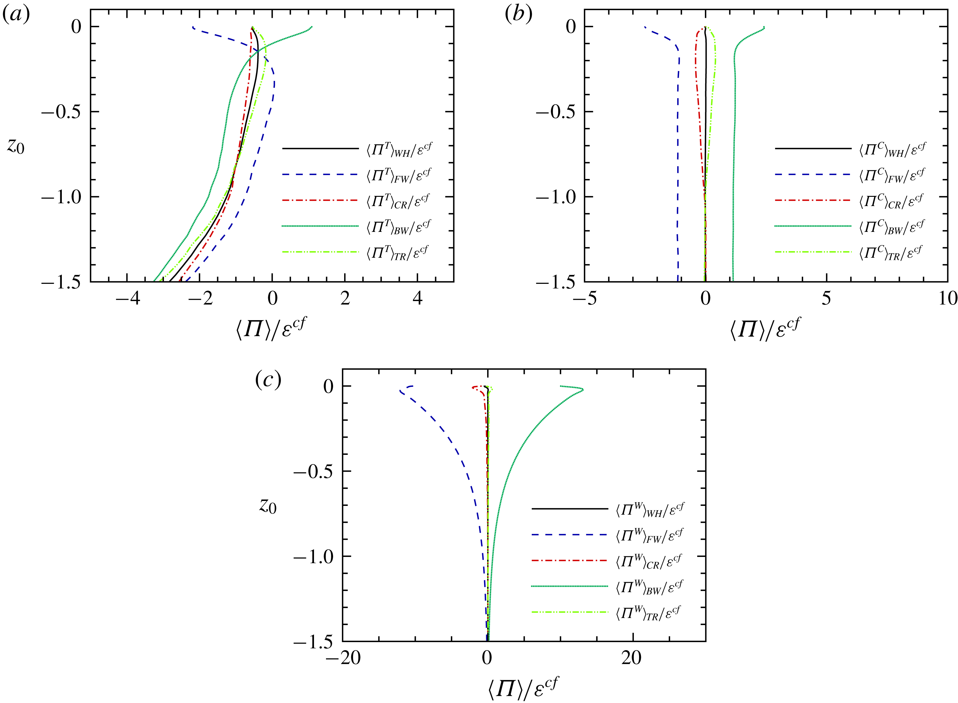
From case I: averages of different energy fluxes: (a)  $\langle \unicode[STIX]{x1D6F1}^{T}\rangle$ ; (b)  $\langle \unicode[STIX]{x1D6F1}^{C}\rangle$ ; and (c)  $\langle \unicode[STIX]{x1D6F1}^{W}\rangle$ .

Figure 7 presents the distribution of the averaged energy flux along the depth. The wave shape range dependence of the energy flux is again shown by different average operators. The filter width used here is the same as that in figure 4. From figure 7(a), the turbulent energy flux $\unicode[STIX]{x1D6F1}^{T}$ is strongly wave-shape-dependent. Below $z_{0}=-0.3$ , $\langle \unicode[STIX]{x1D6F1}^{T}\rangle$ is always negative, suggesting the forward energy cascade. Near the centre of the free region $z_{0}=-0.79$ , $\langle \unicode[STIX]{x1D6F1}^{T}\rangle _{WH}$ is very close to $\unicode[STIX]{x1D716}^{cf}$ , indicating that the turbulent energy is cascading into the small scales and dissipated there. Above $z_{0}=-0.3$ , both $\langle \unicode[STIX]{x1D6F1}^{T}\rangle _{FW}$ and $\langle \unicode[STIX]{x1D6F1}^{T}\rangle _{BW}$ change rapidly, reflecting the blockage effect of the free surface (Hunt & Graham Reference Hunt and Graham1978; Walker, Leighton & Garza-Rios Reference Walker, Leighton and Garza-Rios1996; Shen et al. Reference Shen, Zhang, Yue and Triantafyllou1999). Note that the thickness of the blockage layer ( $z_{0}>-0.3$ ) is very close to the filter width because only the eddies whose sizes are larger than the depth can sense the free surface (Hunt & Graham Reference Hunt and Graham1978). Furthermore, $\langle \unicode[STIX]{x1D6F1}^{T}\rangle _{BW}$ is positive very close to the free surface ( $z_{0}>-0.1$ ).

Figure 7(b,c) show that the energy flux due to the cross-term, $\unicode[STIX]{x1D6F1}^{C}$ , and the wave-induced energy flux, $\unicode[STIX]{x1D6F1}^{W}$ , are also strongly phase-dependent. Flux $\unicode[STIX]{x1D6F1}^{W}$ will be decomposed into $\unicode[STIX]{x1D6F1}_{T}^{W}$ and $\unicode[STIX]{x1D6F1}_{W}^{W}$ in (3.24). On the one hand, the phase average of $\unicode[STIX]{x1D6F1}_{T}^{W}$ vanishes because $\unicode[STIX]{x1D6F1}_{T}^{W}\equiv \langle \unicode[STIX]{x1D70F}_{ij}^{W}\tilde{\unicode[STIX]{x1D61A}}_{ij}^{T}\rangle =\unicode[STIX]{x1D70F}_{ij}^{W}\langle \tilde{\unicode[STIX]{x1D61A}}_{ij}^{T}\rangle$ and $\langle \tilde{\unicode[STIX]{x1D61A}}_{ij}^{T}\rangle =0$ , where $\tilde{\unicode[STIX]{x1D61A}}_{ij}^{T}$ is the turbulent part of the strain-rate tensor. On the other hand, $\unicode[STIX]{x1D6F1}_{W}^{W}$ will be found in § 4 transferring energy between large-scale wave motion ( $\widetilde{u_{i}^{W}}\widetilde{u_{i}^{W}}$ ) and small-scale wave motion ( $\unicode[STIX]{x1D70F}_{ii}^{W}$ ), which leads to the negligible magnitude of $\langle \unicode[STIX]{x1D6F1}_{W}^{W}\rangle _{WH}$ . Therefore, $\langle \unicode[STIX]{x1D6F1}^{W}\rangle _{WH}$ is very close to zero. The value of $\langle \unicode[STIX]{x1D6F1}^{C}\rangle _{WH}$ almost vanishes as well at any depth, indicating that the cross-interaction energy flux makes no contribution to the net energy cascade when integrated over one wave period.

Note that the Lagrangian average along the trajectory of a wave particle is applied. For example, $\langle \unicode[STIX]{x1D6F1}^{W}\rangle _{WH}$ is the average of $\langle \unicode[STIX]{x1D6F1}^{W}\rangle$ when the wave particle passes through one wavelength. The fact that $\langle \unicode[STIX]{x1D6F1}^{W}\rangle _{WH}$ and $\langle \unicode[STIX]{x1D6F1}^{C}\rangle _{WH}$ are quite close to zero does not contradict the cumulative effect of the wave straining. A brief explanation is provided here. Previous works (Teixeira & Belcher Reference Teixeira and Belcher2002; Guo & Shen Reference Guo and Shen2013) show that $\unicode[STIX]{x2202}u^{W}/\unicode[STIX]{x2202}z$ or $\unicode[STIX]{x2202}w^{W}/\unicode[STIX]{x2202}x$ has significant Lagrangian average over one wave period, which is the same order as $ak_{W}S$ , where $S=ak_{W}\unicode[STIX]{x1D714}$ is the magnitude of the wave straining. What is more, it is well known that the Lagrangian average of $u$ , also called the Stokes drift $u_{S}$ , is $ak_{W}(a\unicode[STIX]{x1D714})\exp (2k_{W}z)$ . We can see that the ratio of the cumulative increments of these variables over one wave period to their magnitude is approximately $ak_{W}$ . However, for any variable (i.e.  $\unicode[STIX]{x2202}u^{W}/\unicode[STIX]{x2202}x$ or $w^{W}$ ) whose phase dependence does not have the same harmonic mode as $u^{W}$ , it will be shown that the ratio is at most $O((ak_{W})^{2})$ . Thus its cumulative increment is negligible within one wave period. Take the variable $f(x,z,t)=\exp (lk_{W}z)[\sin (m(k_{W}x+\unicode[STIX]{x1D714}t))+\cos (n(k_{W}x+\unicode[STIX]{x1D714}t))]$ as an example, where $l$ ,  $m$ and $n$ are some integers. The symbol $\overline{(\cdot )}$ is used to represent the average in time whose duration is exactly one wave period. Therefore, $\overline{f(x,z,t)}$ equals 0. The Lagrangian average of $f$ over one wave period is $\bar{f}^{L}=\overline{f(x_{L},z_{L},t)}$ , where $x_{L}$ and $z_{L}$ are the coordinates of the wave particle. The expression for $\bar{f}^{L}$ can also be obtained by

(3.13) $$\begin{eqnarray}\displaystyle \bar{f}^{L} & = & \displaystyle \overline{f(x_{L},z_{L},t)}-\overline{f(x,z,t)}\nonumber\\ \displaystyle & {\approx} & \displaystyle \overline{\frac{\unicode[STIX]{x2202}f}{\unicode[STIX]{x2202}x}(x_{L}-x)+\frac{\unicode[STIX]{x2202}f}{\unicode[STIX]{x2202}z}(z_{L}-z)}+O((ak_{W})^{2}).\end{eqnarray}$$

The Lagrangian coordinates in the second line of (3.13) can be replaced by $x_{L}=x+a\exp (k_{W}z)\cos (k_{W}x+\unicode[STIX]{x1D714}t)+O(a^{2}k_{W})$ and $z_{L}=z+a\exp (k_{W}z)\sin (k_{W}x+\unicode[STIX]{x1D714}t)+O(a^{2}k_{W})$ . The average in the second line of (3.13) will not be zero if and only if  $m=1$ .

We found that the ratio of $\langle \unicode[STIX]{x1D6F1}^{C}\rangle _{WH}$ to $\langle \unicode[STIX]{x1D6F1}^{C}\rangle _{FW}$ or $\langle \unicode[STIX]{x1D6F1}^{C}\rangle _{BW}$ is approximately $0.5\times 10^{-2}$ and the ratio of $\langle \unicode[STIX]{x1D6F1}^{W}\rangle _{WH}$ to $\langle \unicode[STIX]{x1D6F1}^{W}\rangle _{FW}$ or $\langle \unicode[STIX]{x1D6F1}^{W}\rangle _{BW}$ is approximately $10^{-4}$ . These ratios are less than $(ak_{W})^{2}$ , which indicates that both $\langle \unicode[STIX]{x1D6F1}^{C}\rangle$ and $\langle \unicode[STIX]{x1D6F1}^{W}\rangle$ do not contain the harmonic mode $\sin (k_{W}x+\unicode[STIX]{x1D714}t)$ . In fact, from (3.31) to (3.33), the phase dependence of $\langle \unicode[STIX]{x1D6F1}^{W}\rangle$ can be obtained as $\cos (3(k_{W}x+\unicode[STIX]{x1D714}t))$ .

Figure 8.

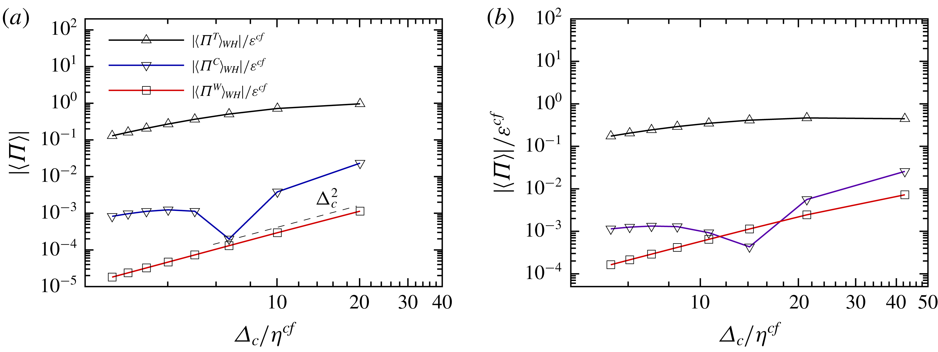
Average of absolute value of the energy flux: (a) averaged over the whole wavelength at $z_{0}=-0.6$ , from case I; and (b) averaged over the whole wavelength at $z_{0}=-0.6$ , from case II.

The filter-width dependence of the energy flux is shown in figure 8. To examine if a power-law behaviour exists, only the magnitude of the averaged energy flux is considered. Note specifically that $\langle \unicode[STIX]{x1D6F1}^{C}\rangle$ changes sign when the filter width decreases, resulting in a cusp in the curve of $|\langle \unicode[STIX]{x1D6F1}^{C}\rangle |$ and no scaling law is expected for it. It is plotted for a comparison of its magnitude with those of $\langle \unicode[STIX]{x1D6F1}^{T}\rangle$ and $\langle \unicode[STIX]{x1D6F1}^{W}\rangle$ . For high-Reynolds-number turbulence, the turbulent energy flux should be equal to the dissipation rate when the SGS kinetic energy is in equilibrium and the filter width is in the inertial range (Meneveau & Katz Reference Meneveau and Katz2000). In case I (figure 8 a), however, $|\langle \unicode[STIX]{x1D6F1}^{T}\rangle _{WH}|$ at $z_{0}=-0.6$ decreases monotonically with decreasing filter width; no plateau is found because of the low $Re_{\unicode[STIX]{x1D706}}$ there. At this depth, $|\langle \unicode[STIX]{x1D6F1}^{C}\rangle _{WH}|$ and $|\langle \unicode[STIX]{x1D6F1}^{W}\rangle _{WH}|$ are at least 10 times smaller than $|\langle \unicode[STIX]{x1D6F1}^{T}\rangle _{WH}|$ . In case II at $z_{0}=-0.6$ (figure 8 b) $|\langle \unicode[STIX]{x1D6F1}^{T}\rangle _{WH}|$ is almost constant between $\unicode[STIX]{x1D6E5}_{c}=14\unicode[STIX]{x1D702}^{cf}$ and $\unicode[STIX]{x1D6E5}_{c}=42\unicode[STIX]{x1D702}^{cf}$ . These results indicate that, for turbulence under strong wave straining, there still exists a range of filter width in which the energy flux is a constant if the Reynolds number is high enough.

In general, the magnitudes of the SGS stress terms and the energy flux terms except $\unicode[STIX]{x1D6F1}^{T}$ in the inertial range depend strongly on the filter width, the turbulent statistics and the properties of the wave-induced motion. In the real world, their orders of magnitude could be quite different from the present situation. Estimations of the magnitude of $\unicode[STIX]{x1D70F}_{ii}^{T}$ and $\unicode[STIX]{x1D70F}_{ii}^{W}$ are thus needed to evaluate their relative importance. Although some deviations from the Kolmogorov scaling exist in figure 6, it is found that $\langle |\unicode[STIX]{x1D70F}_{ii}^{T}|\rangle _{WH}/(\unicode[STIX]{x1D716}\unicode[STIX]{x1D6E5}_{c})^{2/3}$ is between 0.5 and 1 in the free region if $\unicode[STIX]{x1D6E5}_{c}\geqslant 10\unicode[STIX]{x1D702}$ , where $\unicode[STIX]{x1D716}$ is the dissipation obtained at the same depth as $\unicode[STIX]{x1D70F}_{ii}^{T}$ . In other words, $(\unicode[STIX]{x1D716}\unicode[STIX]{x1D6E5}_{c})^{2/3}$ is a rough but reasonable estimation of the magnitude of $\unicode[STIX]{x1D70F}_{ii}^{T}$ even though the Reynolds number is not high enough and the flow is anisotropic.

Since the wave in the present study has a small wave steepness ( $ak_{W}=0.1$ ) and is dominant relative to the turbulence, a linear deep-water wave should be able to describe the wave-induced motion, that is,

(3.14) $$\begin{eqnarray}\left.\begin{array}{@{}c@{}}\displaystyle u^{LW}=-\unicode[STIX]{x1D714}a\exp (k_{W}z)\sin (k_{W}x+\unicode[STIX]{x1D714}t),\\ \displaystyle w^{LW}=\unicode[STIX]{x1D714}a\exp (k_{W}z)\cos (k_{W}x+\unicode[STIX]{x1D714}t),\end{array}\right\}\end{eqnarray}$$

where the superscript ‘ $LW$ ’ denotes ‘linear wave’. Applying the one-dimensional Gaussian filter $G(x)=(\sqrt{6}/\sqrt{\unicode[STIX]{x03C0}}\unicode[STIX]{x1D6E5}_{c})\exp (-6x^{2}/\unicode[STIX]{x1D6E5}_{c}^{2})$ to (3.14), the wave-induced stress components are

(3.15) $$\begin{eqnarray}\displaystyle \unicode[STIX]{x1D70F}_{11}^{LW} & = & \displaystyle (\unicode[STIX]{x1D714}a)^{2}\exp [2k_{W}z]\left[1+\cos (2k_{W}x+2\unicode[STIX]{x1D714}t)\exp \left(-\frac{\unicode[STIX]{x1D6E5}_{c}^{2}}{12}k_{W}^{2}\right)\right]\nonumber\\ \displaystyle & & \displaystyle \times \,\left[1-\exp \left(-\frac{\unicode[STIX]{x1D6E5}_{c}^{2}}{24}k_{W}^{2}\right)\right],\end{eqnarray}$$

(3.16) $$\begin{eqnarray}\displaystyle \unicode[STIX]{x1D70F}_{33}^{LW} & = & \displaystyle (\unicode[STIX]{x1D714}a)^{2}\exp [2k_{W}z]\left[1-\cos (2k_{W}x+2\unicode[STIX]{x1D714}t)\exp \left(-\frac{\unicode[STIX]{x1D6E5}_{c}^{2}}{12}k_{W}^{2}\right)\right]\nonumber\\ \displaystyle & & \displaystyle \times \,\left[1-\exp \left(-\frac{\unicode[STIX]{x1D6E5}_{c}^{2}}{24}k_{W}^{2}\right)\right],\end{eqnarray}$$

(3.17) $$\begin{eqnarray}\displaystyle \unicode[STIX]{x1D70F}_{13}^{LW} & = & \displaystyle (\unicode[STIX]{x1D714}a)^{2}\exp [2k_{W}z]\left[\sin (2k_{W}x+2\unicode[STIX]{x1D714}t)\exp \left(-\frac{\unicode[STIX]{x1D6E5}_{c}^{2}}{12}k_{W}^{2}\right)\right]\nonumber\\ \displaystyle & & \displaystyle \times \,\left[1-\exp \left(-\frac{\unicode[STIX]{x1D6E5}_{c}^{2}}{24}k_{W}^{2}\right)\right],\end{eqnarray}$$

and $\unicode[STIX]{x1D70F}_{12}^{LW}=\unicode[STIX]{x1D70F}_{22}^{LW}=\unicode[STIX]{x1D70F}_{23}^{LW}=0$ . The exponential decay rate of the wave-induced stress is twice that of the wave-induced motion, and the wavenumber is also doubled. When the filter width is much smaller than the wavelength ( $\unicode[STIX]{x1D6E5}_{c}k_{W}\ll 1$ ), $1-\exp (-\unicode[STIX]{x1D6E5}_{c}^{2}k_{W}^{2}/24)$ on the right-hand side of (3.15)–(3.17) equals $\unicode[STIX]{x1D6E5}_{c}^{2}k_{W}^{2}/24$ asymptotically. This $\unicode[STIX]{x1D6E5}_{c}^{2}$ scaling of $\unicode[STIX]{x1D70F}_{ii}^{W}$ is clearly seen in figure 6. From the Kolmogorov scaling and the linear wave theory, the ratio of $O(\unicode[STIX]{x1D70F}_{ii}^{T})$ to $O(\unicode[STIX]{x1D70F}_{ii}^{W})$ is estimated as

(3.18) $$\begin{eqnarray}\frac{O(\unicode[STIX]{x1D70F}_{ii}^{T})}{O(\unicode[STIX]{x1D70F}_{ii}^{W})}\approx \frac{(\unicode[STIX]{x1D716}\unicode[STIX]{x1D6E5}_{c})^{2/3}}{2(\unicode[STIX]{x1D714}a)^{2}\exp (2k_{W}z)\unicode[STIX]{x1D6E5}_{c}^{2}k_{W}^{2}/24}=\frac{27}{\exp (2k_{W}z)}\left(\frac{L_{\infty }}{\unicode[STIX]{x1D6E5}_{c}}\right)^{4/3}\frac{1}{(Sq/\unicode[STIX]{x1D716})^{2}}.\end{eqnarray}$$

In the deep region where $\exp (2k_{W}z)$ tends to zero, $O(\unicode[STIX]{x1D70F}_{ii}^{T})/O(\unicode[STIX]{x1D70F}_{ii}^{W})\gg 1$ , as the case in figure 6(a). In case I at the depth $z^{cf}$ , introducing $\exp (2k_{W}z^{cf})$ , $L_{\infty }^{cf}/\unicode[STIX]{x1D6E5}_{c}$ and $Sq^{cf}/\unicode[STIX]{x1D716}^{cf}$ into (3.18), $O(\unicode[STIX]{x1D70F}_{ii}^{cf,T})/O(\unicode[STIX]{x1D70F}_{ii}^{cf,W})=3.5$ ; while the results from figure 4(a) show that $\langle \unicode[STIX]{x1D70F}_{ii}^{cf,T}\rangle _{WH}/\langle \unicode[STIX]{x1D70F}_{ii}^{cf,W}\rangle _{WH}=2.6$ . Considering that $(\unicode[STIX]{x1D716}\unicode[STIX]{x1D6E5}_{c})^{2/3}$ may overestimate $\unicode[STIX]{x1D70F}_{ii}^{T}$ , the difference between the estimated ratio of $3.5$ and the numerical one of $2.6$ is acceptable.

Figure 9.

Plot of $Sq/\unicode[STIX]{x1D716}$ against $\unicode[STIX]{x1D6E5}_{c}/L_{\infty }$ . Here $R$ is the last expression in (3.18) with $z=0$ .

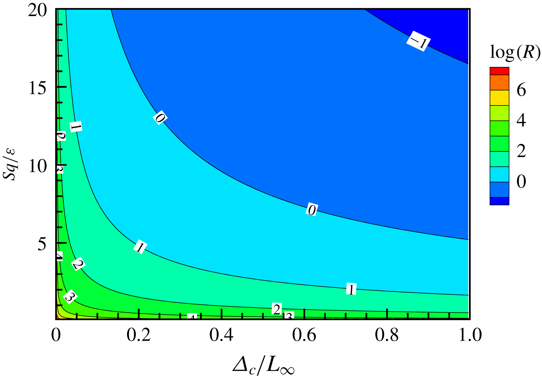
Since the magnitude ratio of turbulent SGS stress to wave-induced SGS stress in (3.18) is proportional to $(\unicode[STIX]{x1D6E5}_{c}/L_{\infty })^{-4/3}$ and $(Sq/\unicode[STIX]{x1D716})^{-2}$ , the wave-induced SGS stress could be comparable to the turbulent SGS stress and has to be modelled appropriately in LES when the filter width is large or the wave straining is strong (i.e. the region to the right of the contour line 1 in figure 9). Whether a filter is fine enough to remove the wave-induced SGS stress needs to be discussed in a specific situation. For example, if turbulent statistics at depth $z^{cf}$ in case I are introduced to (3.18), a filter would be less than $0.22L_{\infty }^{cf}=0.023\unicode[STIX]{x1D6EC}$ to make $\unicode[STIX]{x1D70F}_{ii}^{W}$ no more than $10\,\%$ of $\unicode[STIX]{x1D70F}_{ii}^{T}$ . Turbulence near the surface of the ocean usually originates from wind stress if a breaking wave is absent. Based on the observation in Anis & Moum (Reference Anis and Moum1995), Huang & Qiao (Reference Huang and Qiao2010) proposed a model describing the dissipation rate $\unicode[STIX]{x1D700}_{w}$ induced by wave–turbulence interaction:

(3.19) $$\begin{eqnarray}\unicode[STIX]{x1D700}_{w}=148\unicode[STIX]{x1D6FD}\sqrt{\frac{2a}{L}}\frac{u_{s0}u_{\ast }^{2}}{L}\exp (2kz),\end{eqnarray}$$

where $a$ is related to the significant wave height by $a=H_{s}/2$ ; $\unicode[STIX]{x1D6FD}$ is a dimensionless coefficient less than 1; $L$ is the wavelength; $u_{s0}~(=\unicode[STIX]{x1D714}ka^{2})$ is the Stokes drift at the free surface; and $u_{\ast }^{2}=\unicode[STIX]{x1D70F}_{0}/\unicode[STIX]{x1D70C}$ . Here $\unicode[STIX]{x1D70F}_{0}$ is the surface wind stress and $\unicode[STIX]{x1D70C}$ is the density of the sea water. Assuming that the Kolmogorov scaling is still valid in this case, by introducing (3.19) and $\unicode[STIX]{x1D714}^{2}=gk$ into the second expression in (3.18), the following expression is obtained:

(3.20) $$\begin{eqnarray}\frac{O(\unicode[STIX]{x1D70F}_{ii}^{T})}{O(\unicode[STIX]{x1D70F}_{ii}^{W})}=2.15\exp \left(-\frac{2k_{W}z}{3}\right)\unicode[STIX]{x1D6FD}^{2/3}\left(\frac{gu_{\ast }^{4}}{H_{s}\unicode[STIX]{x1D6E5}_{c}^{4}}\right)^{1/3}T^{2},\end{eqnarray}$$

where $T~(=2\unicode[STIX]{x03C0}/\unicode[STIX]{x1D714})$ is the wave period. If $O(\unicode[STIX]{x1D70F}_{ii}^{W})$ is required to be no more than $10\,\%$ of $O(\unicode[STIX]{x1D70F}_{ii}^{T})$ , equation (3.20) gives the following criterion:

(3.21) $$\begin{eqnarray}\unicode[STIX]{x1D6E5}_{c}\leqslant 0.215\exp \left(-\frac{k_{W}z}{2}\right)\unicode[STIX]{x1D6FD}^{1/2}\left(\frac{g}{H_{s}}\right)^{1/4}u_{\ast }T^{3/2}.\end{eqnarray}$$

For case OR90d1 in Huang & Qiao (Reference Huang and Qiao2010), equation (3.21) becomes $\unicode[STIX]{x1D6E5}_{c}\leqslant 0.015$  m, which is approximately $2.70\times 10^{-4}L$ . In other words, to suppress the wave-induced SGS stress to a negligible level, at least $3700$ grids should be allocated in one wavelength!

In (3.10), (3.11) and (3.12), the filtered strain-rate tensor $\tilde{\unicode[STIX]{x1D61A}}_{ij}$ consists of a turbulent part $\tilde{\unicode[STIX]{x1D61A}}_{ij}^{T}$ and a wave-induced part $\tilde{\unicode[STIX]{x1D61A}}_{ij}^{W}$ , so the energy flux can be further decomposed, i.e.

(3.22) $$\begin{eqnarray}\displaystyle & \displaystyle \unicode[STIX]{x1D6F1}^{T}=\unicode[STIX]{x1D6F1}_{T}^{T}+\unicode[STIX]{x1D6F1}_{W}^{T}, & \displaystyle\end{eqnarray}$$

(3.23) $$\begin{eqnarray}\displaystyle & \displaystyle \unicode[STIX]{x1D6F1}^{C}=\unicode[STIX]{x1D6F1}_{T}^{C}+\unicode[STIX]{x1D6F1}_{W}^{C}, & \displaystyle\end{eqnarray}$$

(3.24) $$\begin{eqnarray}\displaystyle & \displaystyle \unicode[STIX]{x1D6F1}^{W}=\unicode[STIX]{x1D6F1}_{T}^{W}+\unicode[STIX]{x1D6F1}_{W}^{W}, & \displaystyle\end{eqnarray}$$

where $\unicode[STIX]{x1D6F1}_{T}^{T}\equiv 2\unicode[STIX]{x1D70F}_{ij}^{T}\tilde{\unicode[STIX]{x1D61A}}_{ij}^{T}$ ,  $\unicode[STIX]{x1D6F1}_{W}^{T}\equiv 2\unicode[STIX]{x1D70F}_{ij}^{T}\tilde{\unicode[STIX]{x1D61A}}_{ij}^{W}$ ,  $\unicode[STIX]{x1D6F1}_{T}^{C}\equiv 2\unicode[STIX]{x1D70F}_{ij}^{C}\tilde{\unicode[STIX]{x1D61A}}_{ij}^{T}$ ,  $\unicode[STIX]{x1D6F1}_{W}^{C}\equiv 2\unicode[STIX]{x1D70F}_{ij}^{C}\tilde{\unicode[STIX]{x1D61A}}_{ij}^{W}$ ,  $\unicode[STIX]{x1D6F1}_{T}^{W}\equiv 2\unicode[STIX]{x1D70F}_{ij}^{W}\tilde{\unicode[STIX]{x1D61A}}_{ij}^{T}$ and $\unicode[STIX]{x1D6F1}_{W}^{W}\equiv 2\unicode[STIX]{x1D70F}_{ij}^{W}\tilde{\unicode[STIX]{x1D61A}}_{ij}^{W}$ .

Figure 10.

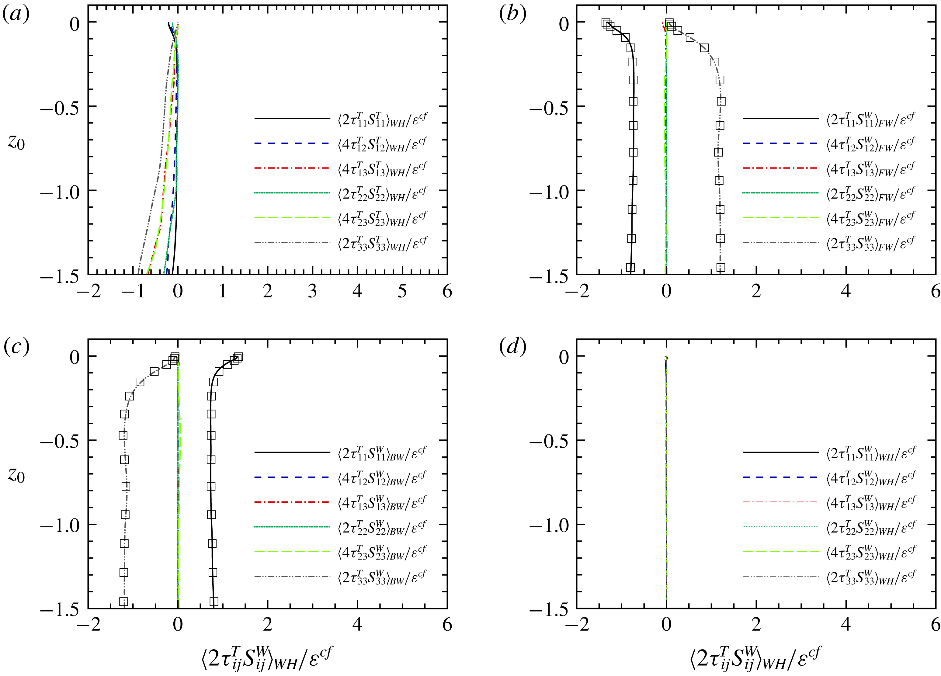
From case I: each component of $\unicode[STIX]{x1D6F1}_{T}^{T}$ and $\unicode[STIX]{x1D6F1}_{W}^{T}$ along the vertical direction: (a) decomposition of $\unicode[STIX]{x1D6F1}_{T}^{T}$ , averaged over the whole wavelength; (b) decomposition of $\unicode[STIX]{x1D6F1}_{W}^{T}$ , averaged over the forward slope range; (c) decomposition of $\unicode[STIX]{x1D6F1}_{W}^{T}$ , averaged over the backward slope range; and (d) decomposition of $\unicode[STIX]{x1D6F1}_{W}^{T}$ , averaged over the whole wavelength.

Here $\unicode[STIX]{x1D6F1}_{T}^{T}$ contains six parts, which are $2\unicode[STIX]{x1D70F}_{11}^{T}S_{11}^{T}$ , $4\unicode[STIX]{x1D70F}_{12}^{T}S_{12}^{T}$ , $4\unicode[STIX]{x1D70F}_{13}^{T}S_{13}^{T}$ , $2\unicode[STIX]{x1D70F}_{22}^{T}S_{22}^{T}$ , $4\unicode[STIX]{x1D70F}_{23}^{T}S_{23}^{T}$ and $2\unicode[STIX]{x1D70F}_{33}^{T}S_{33}^{T}$ . Figure 10(a) shows the averaged value of each component along the vertical direction. For the averages over other wave shape ranges (not shown), the curves are nearly the same, suggesting again that the turbulent statistics are weakly phase-dependent. It is interesting to see that each component has a negative averaged value, so an eddy-viscosity model may be suitable to relate $\unicode[STIX]{x1D61A}_{ij}^{T}$ and $\unicode[STIX]{x1D70F}_{ij}^{T}$ . But the model coefficient should be taken as a tensor because of anisotropy.

Also $\unicode[STIX]{x1D6F1}_{W}^{T}$ consists of six parts, $2\unicode[STIX]{x1D70F}_{11}^{T}S_{11}^{W}$ , $4\unicode[STIX]{x1D70F}_{12}^{T}S_{12}^{W}$ , $4\unicode[STIX]{x1D70F}_{13}^{T}S_{13}^{W}$ , $2\unicode[STIX]{x1D70F}_{22}^{T}S_{22}^{W}$ , $4\unicode[STIX]{x1D70F}_{23}^{T}S_{23}^{W}$ and $2\unicode[STIX]{x1D70F}_{33}^{T}S_{33}^{W}$ , which are presented in figure 10(b–d). From (3.14) the linear wave has strain-rate tensor as

(3.25) $$\begin{eqnarray}\displaystyle & \displaystyle \tilde{\unicode[STIX]{x1D61A}}_{11}^{LW}=-\unicode[STIX]{x1D714}ak_{W}\exp (k_{W}z)\cos (k_{W}x+\unicode[STIX]{x1D714}t)\exp \left(-\frac{\unicode[STIX]{x1D6E5}_{c}^{2}}{24}k_{W}^{2}\right), & \displaystyle\end{eqnarray}$$

(3.26) $$\begin{eqnarray}\displaystyle & \displaystyle \tilde{\unicode[STIX]{x1D61A}}_{33}^{LW}=\unicode[STIX]{x1D714}ak_{W}\exp (k_{W}z)\cos (k_{W}x+\unicode[STIX]{x1D714}t)\exp \left(-\frac{\unicode[STIX]{x1D6E5}_{c}^{2}}{24}k_{W}^{2}\right), & \displaystyle\end{eqnarray}$$

(3.27) $$\begin{eqnarray}\displaystyle & \displaystyle \tilde{\unicode[STIX]{x1D61A}}_{13}^{LW}=-\unicode[STIX]{x1D714}ak_{W}\exp (k_{W}z)\sin (k_{W}x+\unicode[STIX]{x1D714}t)\exp \left(-\frac{\unicode[STIX]{x1D6E5}_{c}^{2}}{24}k_{W}^{2}\right), & \displaystyle\end{eqnarray}$$

and $\tilde{\unicode[STIX]{x1D61A}}_{12}^{LW}=\tilde{\unicode[STIX]{x1D61A}}_{22}^{LW}=\tilde{\unicode[STIX]{x1D61A}}_{23}^{LW}=0$ . Figure 10(b,c) show that $4\unicode[STIX]{x1D70F}_{12}^{T}\tilde{\unicode[STIX]{x1D61A}}_{12}^{W}$ , $2\unicode[STIX]{x1D70F}_{22}^{T}\tilde{\unicode[STIX]{x1D61A}}_{22}^{W}$ and $4\unicode[STIX]{x1D70F}_{23}^{T}\tilde{\unicode[STIX]{x1D61A}}_{23}^{W}$ are close to zero at any depth and over any wave shape range, implying that $\tilde{\unicode[STIX]{x1D61A}}_{12}^{W}$ , $\tilde{\unicode[STIX]{x1D61A}}_{22}^{W}$ and $\tilde{\unicode[STIX]{x1D61A}}_{23}^{W}$ are close to zero, consistent with the linear wave theory. Because the surface is free of tangential stress, $\langle \unicode[STIX]{x1D70F}_{13}^{T}\rangle$ is much less than $\langle \unicode[STIX]{x1D70F}_{11}^{T}\rangle$ and $\langle \unicode[STIX]{x1D70F}_{33}^{T}\rangle$ and the shear component of the energy flux is much smaller than the normal components. With the help of (3.25), (3.26) and (3.27), $\langle 2\unicode[STIX]{x1D70F}_{11}^{T}\tilde{\unicode[STIX]{x1D61A}}_{11}^{W}\rangle$ , $\langle 2\unicode[STIX]{x1D70F}_{33}^{T}\tilde{\unicode[STIX]{x1D61A}}_{33}^{W}\rangle$ and $\langle \unicode[STIX]{x1D6F1}_{W}^{T}\rangle$ can be estimated as follows:

(3.28) $$\begin{eqnarray}\displaystyle & \displaystyle \langle 2\unicode[STIX]{x1D70F}_{11}^{T}\tilde{\unicode[STIX]{x1D61A}}_{11}^{W}\rangle \approx -2\langle \unicode[STIX]{x1D70F}_{11}^{T}\rangle \unicode[STIX]{x1D714}ak_{W}\exp (k_{W}z)\cos (k_{W}x+\unicode[STIX]{x1D714}t)\times \exp \left(-\frac{\unicode[STIX]{x1D6E5}_{c}^{2}}{24}k_{W}^{2}\right), & \displaystyle\end{eqnarray}$$

(3.29) $$\begin{eqnarray}\displaystyle & \displaystyle \langle 2\unicode[STIX]{x1D70F}_{33}^{T}\tilde{\unicode[STIX]{x1D61A}}_{33}^{W}\rangle \approx 2\langle \unicode[STIX]{x1D70F}_{33}^{T}\rangle \unicode[STIX]{x1D714}ak_{W}\exp (k_{W}z)\cos (k_{W}x+\unicode[STIX]{x1D714}t)\times \exp \left(-\frac{\unicode[STIX]{x1D6E5}_{c}^{2}}{24}k_{W}^{2}\right), & \displaystyle\end{eqnarray}$$

and

(3.30) $$\begin{eqnarray}\langle \unicode[STIX]{x1D6F1}_{W}^{T}\rangle \approx 2(\langle \unicode[STIX]{x1D70F}_{33}^{T}\rangle -\langle \unicode[STIX]{x1D70F}_{11}^{T}\rangle )\unicode[STIX]{x1D714}ak_{W}\exp (k_{W}z)\cos (k_{W}x+\unicode[STIX]{x1D714}t)\times \exp \left(-\frac{\unicode[STIX]{x1D6E5}_{c}^{2}}{24}k_{W}^{2}\right).\end{eqnarray}$$

The above estimations in (3.28) and (3.29) are shown by square symbols in figure 10(b,c) and are in good agreement with the DNS results. If the turbulence was isotropic, i.e.  $\unicode[STIX]{x1D70F}_{11}^{T}=\unicode[STIX]{x1D70F}_{33}^{T}$ , then $\unicode[STIX]{x1D6F1}_{W}^{T}$ would be negligible everywhere. However, due to the blockage effect of the free surface, the turbulent kinetic energy is transferred from the vertical component to the horizontal components (see Shen & Yue Reference Shen and Yue2001), leading to $\unicode[STIX]{x1D70F}_{11}^{T}>\unicode[STIX]{x1D70F}_{33}^{T}$ . Hence $\langle \unicode[STIX]{x1D6F1}_{W}^{T}\rangle _{FW}<0$ (respectively $\langle \unicode[STIX]{x1D6F1}_{W}^{T}\rangle _{BW}>0$ ) within the blockage layer. That is why $\langle \unicode[STIX]{x1D6F1}^{T}\rangle _{BW}~(=\langle \unicode[STIX]{x1D6F1}_{W}^{T}\rangle _{BW}+\langle \unicode[STIX]{x1D6F1}_{T}^{T}\rangle _{BW})>0$ near the free surface (see figure 7 a). When the components of $\unicode[STIX]{x1D6F1}_{W}^{T}$ are averaged over the whole wavelength, all of them vanish (see figure 10 d), once again indicating the weak wave shape range dependence of the turbulent statistics.

Regarding $\unicode[STIX]{x1D6F1}^{W}$ , it is found that the average value of $\unicode[STIX]{x1D6F1}_{T}^{W}$ is negligible, because 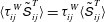$\langle \unicode[STIX]{x1D70F}_{ij}^{W}\tilde{\unicode[STIX]{x1D61A}}_{ij}^{T}\rangle =\unicode[STIX]{x1D70F}_{ij}^{W}\langle \tilde{\unicode[STIX]{x1D61A}}_{ij}^{T}\rangle$ and $\langle \tilde{\unicode[STIX]{x1D61A}}_{ij}^{T}\rangle =0$ . Similar to $\unicode[STIX]{x1D6F1}_{T}^{T}$ , $\unicode[STIX]{x1D6F1}_{W}^{W}$ can also be decomposed into six components. The numerical results for the six components are not shown because they can be well estimated by combining (3.15)–(3.17) with (3.25)–(3.27):

(3.31) $$\begin{eqnarray}\displaystyle 2\unicode[STIX]{x1D70F}_{11}^{W}\tilde{\unicode[STIX]{x1D61A}}_{11}^{W} & {\approx} & \displaystyle 2\unicode[STIX]{x1D70F}_{11}^{LW}\tilde{\unicode[STIX]{x1D61A}}_{11}^{LW}\nonumber\\ \displaystyle & = & \displaystyle -2(\unicode[STIX]{x1D714}a)^{3}k_{W}\exp (3k_{W}z)\cos (k_{W}x+\unicode[STIX]{x1D714}t)\nonumber\\ \displaystyle & & \displaystyle \times \,\left[1+\cos (2k_{W}x+2\unicode[STIX]{x1D714}t)\exp \left(-\frac{\unicode[STIX]{x1D6E5}_{c}^{2}}{12}k_{W}^{2}\right)\right]\nonumber\\ \displaystyle & & \displaystyle \times \,\left[1-\exp \left(-\frac{\unicode[STIX]{x1D6E5}_{c}^{2}}{24}k_{W}^{2}\right)\right],\end{eqnarray}$$

(3.32) $$\begin{eqnarray}\displaystyle 2\unicode[STIX]{x1D70F}_{33}^{W}\tilde{\unicode[STIX]{x1D61A}}_{33}^{W} & {\approx} & \displaystyle 2\unicode[STIX]{x1D70F}_{33}^{LW}\tilde{\unicode[STIX]{x1D61A}}_{33}^{LW}\nonumber\\ \displaystyle & = & \displaystyle 2(\unicode[STIX]{x1D714}a)^{3}k_{W}\exp (3k_{W}z)\cos (k_{W}x+\unicode[STIX]{x1D714}t)\nonumber\\ \displaystyle & & \displaystyle \times \,\left[1-\cos (2k_{W}x+2\unicode[STIX]{x1D714}t)\exp \left(-\frac{\unicode[STIX]{x1D6E5}_{c}^{2}}{12}k_{W}^{2}\right)\right]\nonumber\\ \displaystyle & & \displaystyle \times \,\left[1-\exp \left(-\frac{\unicode[STIX]{x1D6E5}_{c}^{2}}{24}k_{W}^{2}\right)\right],\end{eqnarray}$$

(3.33) $$\begin{eqnarray}\displaystyle 4\unicode[STIX]{x1D70F}_{13}^{W}\tilde{\unicode[STIX]{x1D61A}}_{13}^{W} & {\approx} & \displaystyle 4\unicode[STIX]{x1D70F}_{13}^{LW}\tilde{\unicode[STIX]{x1D61A}}_{13}^{LW}\nonumber\\ \displaystyle & = & \displaystyle 4(\unicode[STIX]{x1D714}a)^{3}k_{W}\exp (3k_{W}z)\sin (k_{W}x+\unicode[STIX]{x1D714}t)\sin (2k_{W}x+2\unicode[STIX]{x1D714}t)\nonumber\\ \displaystyle & & \displaystyle \times \,\exp \left(-\frac{\unicode[STIX]{x1D6E5}_{c}^{2}}{12}k_{W}^{2}\right)\left[1-\exp \left(-\frac{\unicode[STIX]{x1D6E5}_{c}^{2}}{24}k_{W}^{2}\right)\right],\end{eqnarray}$$

and $4\unicode[STIX]{x1D70F}_{12}^{W}\tilde{\unicode[STIX]{x1D61A}}_{12}^{W}$ ,  $2\unicode[STIX]{x1D70F}_{22}^{W}\tilde{\unicode[STIX]{x1D61A}}_{22}^{W}$ and $4\unicode[STIX]{x1D70F}_{23}^{W}\tilde{\unicode[STIX]{x1D61A}}_{23}^{W}$ are approximately zero. A $\unicode[STIX]{x1D6E5}_{c}^{2}$ scaling emerges if $\unicode[STIX]{x1D6E5}_{c}k_{W}\ll 1$ , which is evident in figure 8. From (3.31) to (3.33), $\langle \unicode[STIX]{x1D6F1}_{W}^{W}\rangle _{WH}=0$ . The integrated contribution of $\unicode[STIX]{x1D6F1}_{W}^{W}$ to the energy flux over one wave period should be essentially zero because $\unicode[STIX]{x1D6F1}_{W}^{W}$ only transfers energy between large-scale wave motion and small-scale wave motion (see the following section). The linear wave theory indicates that the wavenumber of $\unicode[STIX]{x1D70F}_{ij}^{LW}$ is twice the wavenumber of $\tilde{\unicode[STIX]{x1D61A}}_{ij}^{LW}$ (see equations (3.15)–(3.17) and (3.25)–(3.27)). The strain-rate tensor and the SGS stress should have the same wavenumber if they are related by an eddy-viscosity model and the scalar factor in the model has weak dependence on the wave phase. For example, the scalar factor in the Smagorinsky model derived from $\tilde{\unicode[STIX]{x1D61A}}_{ij}^{W}$ is independent of the phase. Therefore, such an eddy-viscosity model is inappropriate to relate $\unicode[STIX]{x1D70F}_{ij}$ with $\tilde{\unicode[STIX]{x1D61A}}_{ij}$ when both $\unicode[STIX]{x1D70F}_{ij}^{W}$ and $\tilde{\unicode[STIX]{x1D61A}}_{ij}^{W}$ are not negligible.

4 Budget equation for the subgrid-scale stress

In the previous section, the energy flux was decomposed into $\unicode[STIX]{x1D6F1}_{T}^{T}$ , $\unicode[STIX]{x1D6F1}_{W}^{T}$ , $\unicode[STIX]{x1D6F1}_{T}^{C}$ , $\unicode[STIX]{x1D6F1}_{W}^{C}$ , $\unicode[STIX]{x1D6F1}_{T}^{W}$ and $\unicode[STIX]{x1D6F1}_{W}^{W}$ , and their wave shape range dependence, vertical variation and scaling law were discussed. However, their roles in the energy transfer between large scales and small scales are still unknown. This question could be answered by considering the budget equations for the kinetic energy of the filtered motion and that of the SGS motion. Given the decomposition of the velocity in (3.2), the kinetic energy of the filtered motion is now

(4.1) $$\begin{eqnarray}\tilde{u} _{i}\tilde{u} _{i}=\widetilde{u_{i}^{W}}\widetilde{u_{i}^{W}}+\widetilde{u_{i}^{T}}\widetilde{u_{i}^{T}}+2\widetilde{u_{i}^{W}}\widetilde{u_{i}^{T}},\end{eqnarray}$$

where $\widetilde{u_{i}^{W}}\widetilde{u_{i}^{W}}$ is the kinetic energy of the filtered wave-induced motion, $\widetilde{u_{i}^{T}}\widetilde{u_{i}^{T}}$ is the kinetic energy of the filtered turbulent motion and $2\widetilde{u_{i}^{W}}\widetilde{u_{i}^{T}}$ is the kinetic energy due to the coupling of the filtered wave-induced motion and the filtered turbulent motion. Since the wave-induced motion is determined in time and phase (space), $\langle 2\widetilde{u_{i}^{W}}\widetilde{u_{i}^{T}}\rangle =2\widetilde{u_{i}^{W}}\langle \widetilde{u_{i}^{T}}\rangle =0$ . On the other hand, the SGS kinetic energy is usually characterized by $\unicode[STIX]{x1D70F}_{ii}$ , which comprises $\unicode[STIX]{x1D70F}_{ii}^{T}$ , $\unicode[STIX]{x1D70F}_{ii}^{C}$ and $\unicode[STIX]{x1D70F}_{ii}^{W}$ . Budget equations (refer to the supplementary material available at https://doi.org/10.1017/jfm.2019.658) for various terms at both resolved scale and subgrid scale show that: $\unicode[STIX]{x1D6F1}_{T}^{T}$ and $\unicode[STIX]{x1D6F1}_{T}^{C}$ transfer energy from $\widetilde{u_{i}^{T}}\widetilde{u_{i}^{T}}$ to $\unicode[STIX]{x1D70F}_{ii}^{T}$ ; $\unicode[STIX]{x1D6F1}_{W}^{T}$ , $\unicode[STIX]{x1D6F1}_{W}^{C}$ and $\unicode[STIX]{x1D6F1}_{T}^{W}$ transfer energy from $2\widetilde{u_{i}^{W}}\widetilde{u_{i}^{T}}$ to $\unicode[STIX]{x1D70F}_{ii}^{C}$ ; and $\unicode[STIX]{x1D6F1}_{W}^{W}$ transfers energy from $\widetilde{u_{i}^{W}}\widetilde{u_{i}^{W}}$ to  $\unicode[STIX]{x1D70F}_{ii}^{W}$ .

If the six kinetic energy terms are classified in terms of the nature of fluid motion behind them, there will be three groups. The first group is the turbulent group, containing $\widetilde{u_{i}^{T}}\widetilde{u_{i}^{T}}$ and $\unicode[STIX]{x1D70F}_{ii}^{T}$ . The second group is the wave-induced group, consisting of $\widetilde{u_{i}^{W}}\widetilde{u_{i}^{W}}$ and $\unicode[STIX]{x1D70F}_{ii}^{W}$ . The last group is the cross-interaction group, which has $2\widetilde{u_{i}^{W}}\widetilde{u_{i}^{T}}$ and $\unicode[STIX]{x1D70F}_{ii}^{C}$ . Evidently, direct energy transfer between scales only occurs within the same group.

It should be noted that the energy transfer between the large scales of one group and the small scales of another group is possible only in the indirect way. The cross-interaction group plays a crucial role in an indirect energy transfer. For example, energy in $\unicode[STIX]{x1D70F}_{ii}^{W}$ (or $\widetilde{u_{i}^{W}}\widetilde{u_{i}^{W}}$ ) could first be transferred into $\unicode[STIX]{x1D70F}_{ii}^{C}$ (or $2\widetilde{u_{i}^{W}}\widetilde{u_{i}^{T}}$ ), and then transferred into $\unicode[STIX]{x1D70F}_{ii}^{T}$ (or $\widetilde{u_{i}^{T}}\widetilde{u_{i}^{T}}$ ). However, the indirect transfer channel is very complex, because many terms appear in the budget equation of $\unicode[STIX]{x1D70F}_{ii}^{C}$ and that of $2\widetilde{u_{i}^{W}}\widetilde{u_{i}^{T}}$ . The detailed analysis of the dynamics of $\unicode[STIX]{x1D70F}_{ii}^{C}$ and $2\widetilde{u_{i}^{W}}\widetilde{u_{i}^{T}}$ will be given in future work.

Since $\unicode[STIX]{x1D70F}_{ii}^{W}$ can be well estimated by (3.15)–(3.17), we shall focus on the dynamics of $\unicode[STIX]{x1D70F}_{ii}^{T}$ , which could be beneficial for the construction of the SGS model. The following is the budget equation for $\unicode[STIX]{x1D70F}_{ii}^{T}$ :

(4.2) $$\begin{eqnarray}\displaystyle \frac{\unicode[STIX]{x2202}\unicode[STIX]{x1D70F}_{ii}^{T}}{\unicode[STIX]{x2202}t} & = & \displaystyle \underbrace{-\frac{\unicode[STIX]{x2202}\unicode[STIX]{x1D70F}_{ii}^{T}\widetilde{u_{k}^{T}}}{\unicode[STIX]{x2202}x_{k}}}_{T}\underbrace{-\frac{\unicode[STIX]{x2202}\widetilde{u_{i}^{T}u_{i}^{T}u_{k}^{T}}}{\unicode[STIX]{x2202}x_{k}}}_{\unicode[STIX]{x1D6E4}}\underbrace{-\frac{2}{\unicode[STIX]{x1D70C}}\left(\widetilde{u_{i}^{T}\frac{\unicode[STIX]{x2202}p^{T}}{\unicode[STIX]{x2202}x_{i}}}-\widetilde{u_{i}^{T}}\widetilde{\frac{\unicode[STIX]{x2202}p^{T}}{\unicode[STIX]{x2202}x_{i}}}\right)}_{\unicode[STIX]{x1D6F7}}\nonumber\\ \displaystyle & & \displaystyle \underbrace{-2\left(\widetilde{u_{i}^{T}\frac{\unicode[STIX]{x2202}u_{i}^{W}u_{k}^{T}}{\unicode[STIX]{x2202}x_{k}}}-\widetilde{u_{i}^{T}}\frac{\unicode[STIX]{x2202}\widetilde{u_{i}^{W}}\widetilde{u_{k}^{T}}}{\unicode[STIX]{x2202}x_{k}}\right)}_{P_{W}}\underbrace{-2\left(\widetilde{u_{i}^{T}\frac{\unicode[STIX]{x2202}u_{i}^{T}u_{k}^{W}}{\unicode[STIX]{x2202}x_{k}}}-\widetilde{u_{i}^{T}}\frac{\unicode[STIX]{x2202}\widetilde{u_{i}^{T}}\widetilde{u_{k}^{W}}}{\unicode[STIX]{x2202}x_{k}}\right)}_{P_{T}}\nonumber\\ \displaystyle & & \displaystyle \underbrace{+2(\widetilde{u_{i}^{T}\frac{\unicode[STIX]{x2202}\langle u_{i}^{T}u_{k}^{T}\rangle }{\unicode[STIX]{x2202}x_{k}}}-\widetilde{u_{i}^{T}}\widetilde{\frac{\unicode[STIX]{x2202}\langle u_{i}^{T}u_{k}^{T}\rangle }{\unicode[STIX]{x2202}x_{k}}})}_{P_{R}}\underbrace{-2\unicode[STIX]{x1D70F}_{ij}^{T}\frac{\unicode[STIX]{x2202}\widetilde{u_{i}^{T}}}{\unicode[STIX]{x2202}x_{j}}}_{-\unicode[STIX]{x1D6F1}_{T}^{T}}\underbrace{-2\unicode[STIX]{x1D70F}_{ij}^{C}\frac{\unicode[STIX]{x2202}u_{i}^{T}}{\unicode[STIX]{x2202}x_{j}}}_{-\unicode[STIX]{x1D6F1}_{T}^{C}}\underbrace{+2\frac{\unicode[STIX]{x2202}\widetilde{u_{i}^{T}}\unicode[STIX]{x1D70F}_{ij}^{T}}{\unicode[STIX]{x2202}x_{j}}}_{T_{T}^{SGS}}\nonumber\\ \displaystyle & & \displaystyle \underbrace{+2\frac{\unicode[STIX]{x2202}\widetilde{u_{i}^{T}\unicode[STIX]{x1D70F}_{ij}^{C}}}{\unicode[STIX]{x2202}x_{j}}}_{T_{C}^{SGS}}\underbrace{-2\unicode[STIX]{x1D708}\left(\widetilde{\frac{\unicode[STIX]{x2202}u_{i}^{T}}{\unicode[STIX]{x2202}x_{j}}\frac{\unicode[STIX]{x2202}x_{i}^{T}}{\unicode[STIX]{x2202}x_{j}}}-\frac{\unicode[STIX]{x2202}\widetilde{u_{i}^{T}}}{\unicode[STIX]{x2202}x_{j}}\frac{\unicode[STIX]{x2202}\widetilde{u_{i}^{T}}}{\unicode[STIX]{x2202}x_{j}}\right)}_{D}\underbrace{+\unicode[STIX]{x1D708}\left(\frac{\unicode[STIX]{x2202}^{2}\widetilde{u_{i}^{T}u_{i}^{T}}}{\unicode[STIX]{x2202}x_{j}^{2}}-\frac{\unicode[STIX]{x2202}^{2}\widetilde{u_{i}^{T}}\widetilde{u_{i}^{T}}}{\unicode[STIX]{x2202}x_{j}^{2}}\right)}_{\unicode[STIX]{x1D716}_{T}^{SGS}}.\end{eqnarray}$$

Figure 11.

From case I: the terms on the right-hand side of (4.2) along the vertical direction: (a)  $\unicode[STIX]{x1D6F7}$ , $P_{W}$ , $P_{T}$ , $P_{R}$ , $-\unicode[STIX]{x1D6F1}_{T}^{C}$ and $T_{C}^{SGS}$ , averaged over the forward slope range; (b)  $\unicode[STIX]{x1D6F7}$ , $P_{W}$ , $P_{T}$ , $P_{R}$ , $-\unicode[STIX]{x1D6F1}_{T}^{C}$ and $T_{C}^{SGS}$ , averaged over the backward slope range; (c)  $\unicode[STIX]{x1D6F7}$ , $P_{W}$ , $P_{T}$ , $P_{R}$ , $-\unicode[STIX]{x1D6F1}_{T}^{C}$ and $T_{C}^{SGS}$ , averaged over the whole wavelength; and (d)  $T$ , $\unicode[STIX]{x1D6E4}$ , $-\unicode[STIX]{x1D6F1}_{T}^{T}$ , $T_{T}^{SGS}$ , $D$ and $\unicode[STIX]{x1D716}_{T}^{SGS}$ , averaged over the whole wavelength.

To facilitate the analysis, the terms appearing on the right-hand side of (4.2) are divided into two groups, according to the degree of wave shape range dependence. The first group, a member of which is strongly wave-shape-range-dependent and has zero whole-wavelength-averaged value, contains $\unicode[STIX]{x1D6F7}$ , $P_{W}$ , $P_{T}$ , $P_{R}$ , $-\unicode[STIX]{x1D6F1}_{T}^{C}$ and $T_{C}^{SGS}$ , as is shown in figure 11(a–c). The second group consists of $T$ , $\unicode[STIX]{x1D6E4}$ , $-\unicode[STIX]{x1D6F1}_{T}^{T}$ , $T_{T}^{SGS}$ , $D$ and $\unicode[STIX]{x1D716}_{T}^{SGS}$ , which are weakly wave-shape-range-dependent. All the members of the second group are directly related to the turbulent motion. The whole-wavelength-averaged values of the members in the second group are plotted in figure 11(d). The curves for $\unicode[STIX]{x1D716}_{T}^{SGS}$ and $T_{T}^{SGS}$ are always negative and the curves for the remaining terms are positive. The summation of the members of the second group is approximately zero. It is obvious that the magnitude of the SGS dissipation term $\unicode[STIX]{x1D716}_{T}^{SGS}$ is larger than that of the energy flux term $-\unicode[STIX]{x1D6F1}_{T}^{T}$ , and the gap between them is compensated by the total effect of the transport terms, $T$ , $\unicode[STIX]{x1D6E4}$ and $T_{T}^{SGS}$ . The importance of the transport terms near the free surface may seem to be obvious, since turbulence in this study is generated in the bulk region. However, since the present study is one of the first studies on SGS modelling, quantifying the relative magnitude of different terms in the budget equation for the turbulent SGS kinetic energy should be valuable to future closure study of the SGS stress.

5 Conclusions and discussion

In the present study, we examine how an isotropic turbulence interacts with an energetic and rapid progressive surface wave and how, as a result, the small-scale turbulent motion is modulated. This interaction is simulated by means of DNS. A partition of the velocity field is used to decompose the SGS stress into three parts, namely, the turbulent part $\unicode[STIX]{x1D70F}_{ij}^{T}$ , the wave-induced part $\unicode[STIX]{x1D70F}_{ij}^{W}$ and the cross-interaction part $\unicode[STIX]{x1D70F}_{ij}^{C}$ . The main conclusions are summarized below.

In the free region, the turbulent SGS stress is found to be least phase-dependent among the three parts of the SGS stress, since the RMV of $\langle \unicode[STIX]{x1D70F}_{ii}^{T}\rangle$ when measured along the wave particle trajectories is $5$ times smaller than those of $\langle \unicode[STIX]{x1D70F}_{ii}^{C}\rangle$ and $\langle \unicode[STIX]{x1D70F}_{ii}^{W}\rangle$ . Comparison of the RV of $\langle \unicode[STIX]{x1D70F}_{11}^{T}\rangle$ with those of $\langle (u_{1}^{T})^{2}\rangle$ predicted by Teixeira & Belcher (Reference Teixeira and Belcher2002) in figure 5(b) indicates that the relative variation of the SGS turbulent motion is similar to that of the turbulent motion of all scales.

The Kolmogorov scaling for the SGS stress, originally proposed for isotropic turbulence, seems to be valid for $\unicode[STIX]{x1D70F}_{ii}^{T}$ , although the turbulence underneath the wave surface is far from the isotropic-turbulence phenomenology. This is consistent with previous work (Liu et al. Reference Liu, Katz and Meneveau1999), which showed the validity of the Kolmogorov scaling for the turbulent SGS stress of a flow subject to axisymmetric straining.

The ratio of the magnitude of $\unicode[STIX]{x1D70F}_{ij}^{T}$ to that of $\unicode[STIX]{x1D70F}_{ij}^{W}$ depends on the depth $z$ , the filter width $\unicode[STIX]{x1D6E5}_{c}$ and the straining ratio $Sq/\unicode[STIX]{x1D716}$ . In locations significantly below the surface, $\unicode[STIX]{x1D70F}_{ij}^{W}$ is much smaller than $\unicode[STIX]{x1D70F}_{ij}^{T}$ and can be ignored in the SGS model. When $\unicode[STIX]{x1D6E5}_{c}$ is not very small or the wave straining is strong, i.e. the region to the left of the contour line 1 in figure 9, $\unicode[STIX]{x1D70F}_{ij}^{W}$ can be comparable to $\unicode[STIX]{x1D70F}_{ij}^{T}$ and must be carefully handled. In the open ocean when the wind stress is small and the dissipation rate is mainly controlled by wave–turbulence interaction (Huang & Qiao Reference Huang and Qiao2010), a useful criterion for the upper bound of the filter width to suppress $\unicode[STIX]{x1D70F}_{ij}^{W}$ to a negligible value is given as (3.21). Using the data of the Oregon coast in summer 1990 (Anis & Moum Reference Anis and Moum1995), which is referred to as OR90d1 and OR90d2 in Huang & Qiao (Reference Huang and Qiao2010), it is found that at least 3000 grids should be allocated within one wavelength, which is almost impracticable. If fewer grids are adopted, one must be aware of the effect of $\unicode[STIX]{x1D70F}_{ij}^{W}$ . The simple analysis indicates that, when performing phase-resolving LES, wave-induced SGS stress is not ignorable by itself. Nevertheless, there are still possibilities that the wave-induced SGS stress is negligible. Here we present an illustrative example. A preferred local grid spacing $\unicode[STIX]{x1D6E5}$ in the LES is in the inertial range, so it is reasonable to assume that $L_{\infty }/\unicode[STIX]{x1D6E5}\geqslant 10$ . According to (3.18), $Sq/\unicode[STIX]{x1D700}$ should be no more than $7.6$ , if the ratio of the magnitude of $\unicode[STIX]{x1D70F}_{ij}^{T}$ to that of $\unicode[STIX]{x1D70F}_{ij}^{W}$ is required to be larger than $10$ at the free surface. Such a requirement of the straining ratio could be satisfied if the Froude number is large enough (i.e. case $\text{III}_{10}$ of Guo & Shen (Reference Guo and Shen2013)), or if the wavelength $\unicode[STIX]{x1D6EC}$ is large enough. In the latter case, when applying the turbulent statistics in Kitaigorodskii & Lumley (Reference Kitaigorodskii and Lumley1983), $\unicode[STIX]{x1D6EC}$ should be at least $6$ times $L_{\infty }$ . In other words, at least $60$ grids are required within one wavelength so that $\unicode[STIX]{x1D70F}_{ij}^{W}$ is negligible, which is not difficult to be satisfied.

As expected, the linear wave theory can describe the wave-induced motion of the numerical simulation, since the wave enforced has a small steepness ( $ak_{W}=0.1$ ), a large length scale compared with turbulence ( $\unicode[STIX]{x1D6EC}/L_{\infty }^{cf}\gg 1$ ) and a strong straining relative to the turbulent straining ( $Sq^{cf}/\unicode[STIX]{x1D700}^{cf}\gg 1$ ). Since $\unicode[STIX]{x1D70F}_{ij}^{W}$ is a quadratic quantity of $u_{i}^{W}$ , while $\tilde{\unicode[STIX]{x1D61A}}_{ij}^{W}$ is a linear quantity of $u_{i}^{W}$ , their wavenumbers are different. Accordingly, when $\unicode[STIX]{x1D70F}_{ij}^{W}$ is not negligible, it is incorrect to relate $\unicode[STIX]{x1D70F}_{ij}~(=\unicode[STIX]{x1D70F}_{ij}^{W}+\unicode[STIX]{x1D70F}_{ij}^{T}+\unicode[STIX]{x1D70F}_{ij}^{C})$ and $\tilde{\unicode[STIX]{x1D61A}}_{ij}~(=\tilde{\unicode[STIX]{x1D61A}}_{ij}^{W}+\tilde{\unicode[STIX]{x1D61A}}_{ij}^{T}+\tilde{\unicode[STIX]{x1D61A}}_{ij}^{C})$ by an eddy-viscosity model. The phase difference between $\unicode[STIX]{x1D70F}_{ij}^{T}$ and $\tilde{\unicode[STIX]{x1D61A}}_{ij}^{W}$ also exists. For example, $\unicode[STIX]{x1D70F}_{11}^{T}$ has its maximum value beneath the crest (see figure 5 b), while $\tilde{\unicode[STIX]{x1D61A}}_{11}^{W}$ reaches its maximum value beneath the backward slope (see (3.25)). Chen et al. (Reference Chen, Meneveau and Katz2006) pointed out that sufficiently small filter width leads to little phase lag between the turbulent SGS stress and the applied cyclic planar straining. In the case of wave straining, the rapid distortion theory (RDT) of Teixeira & Belcher (Reference Teixeira and Belcher2002) where the nonlinear interaction between turbulent eddies is omitted shows that the phase difference between the Reynolds stress and the wave straining is fixed. From figure 11(d), the nonlinearity between the turbulent motions plays an important role in the evolution of the SGS turbulent motion, so it might be hard to derive a theory on the phase difference between $\unicode[STIX]{x1D70F}_{ij}^{T}$ and $\tilde{\unicode[STIX]{x1D61A}}_{ij}^{W}$ . Because the range of the appropriate filter width is greatly limited by the short inertial range in the present study, how the phase difference varies with filter width is still unknown. On the other hand, we find $\langle \tilde{\unicode[STIX]{x1D61A}}_{ij}^{T}\unicode[STIX]{x1D70F}_{ij}^{T}\rangle$ is positive for each component and over each wave shape range, indicating that an eddy-viscosity model is likely to work well when relating $\tilde{\unicode[STIX]{x1D61A}}_{ij}^{T}$ with $\unicode[STIX]{x1D70F}_{ij}^{T}$ . Below the thin Stokes layer, the whole-wavelength average of the turbulent energy flux $\unicode[STIX]{x1D6F1}^{T}$ is negative while those of the wave-induced energy flux $\unicode[STIX]{x1D6F1}^{W}$ and the cross-interaction flux $\unicode[STIX]{x1D6F1}^{C}$ are almost zero. In other words, the net energy transfer over one period is mainly contributed by the turbulent energy flux. Within the local wave shape ranges, however, profiles of the averaged energy fluxes could change dramatically within a thin layer (the blockage layer), in which the turbulent SGS statistics feel the blockage effect of the free surface. The thickness of the blockage layer is around the filter width, i.e. the largest length scale of the SGS turbulence, which is consistent with the RDT (Hunt & Graham Reference Hunt and Graham1978) and the numerical simulations (Walker et al. Reference Walker, Leighton and Garza-Rios1996; Shen et al. Reference Shen, Zhang, Yue and Triantafyllou1999).

Both the kinetic energy of the filtered motion and that of the SGS motion are decomposed into a turbulent part, a coupling part and a wave-induced part, resulting in six terms. The six terms are classified into three groups according to the nature of fluid motion behind them. Comparison of the budget equations for the six terms shows that direct energy transfer only happens within the same group. The budget equations for the turbulent SGS kinetic energy are derived and used to quantify the various transport mechanisms. It is found that the energy flux is not balanced by the SGS energy dissipation due to the vertical transport.

We should be aware of the limitations in the present study, which need to be addressed in future research. The first one is the limitation in Reynolds number, leading to quite a narrow inertial range. So the Kolmogorov scaling inferred in the range should be taken as a preliminary conclusion. Moreover, a monochromatic surface wave might be an oversimplification of the real world. Measurements (Forristall Reference Forristall1981; Kitaigorodskii & Lumley Reference Kitaigorodskii and Lumley1983; He et al. Reference He, Howell and Walsh1993) have shown that the wave-height spectrum in the ocean or a lake span a wide range of frequency, corresponding to wavelengths ranging from $O(1~\text{m})$ to $O(10^{3}~\text{m})$ . Though the parameter setting ( $Sq^{cf}\unicode[STIX]{x1D700}^{cf}\gg 1$ and $L_{\infty }^{cf}/\unicode[STIX]{x1D6EC}\ll 1$ ) can cover an important fraction of the gravity waves in the ocean (Teixeira & Belcher Reference Teixeira and Belcher2002), there could be situations that the setting does not satisfy, i.e. the length scales of wave and turbulence are comparable ( $O(1~\text{m})$ ; Kitaigorodskii & Lumley Reference Kitaigorodskii and Lumley1983), or the wave is quite slow ( $f=O(0.1~\text{Hz})$ ; Forristall Reference Forristall1981; He et al. Reference He, Howell and Walsh1993). To gain a complete understanding of the interaction between wave and turbulence, these two situations must be investigated. Finally, the method to generate the turbulence, although it has been widely used in the literature, is somehow artificial. In the ocean, the turbulence could be produced by the instability of the wind-induced shear flow or the breaking of the surface waves. However, the former is not initially isotropic and the latter is produced very near the free surface.