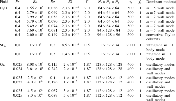
1 Introduction
Rotating Rayleigh–Bénard convection (RBC) is an idealised system that is often invoked to describe the primary physics in a multitude of geo- and astrophysical settings, such as the convective motion occurring in the outer layer of stars, in the oceans, the atmosphere, or in the metallic core of moons and planets. The system itself is deceptively simple – a fluid confined between a heated and a cooled surface, and rotated about its vertical axis. The interplay of the occurring buoyancy and Coriolis forces, however, may yield highly complex flows with very distinct flow structures whose nature strongly depends on the control parameters.
These dimensionless control parameters are the Rayleigh number
 $Ra$
, describing the vigour of the thermal forcing, the Prandtl number
 $Pr$
, a pure material characteristic, and the Ekman number
 $Ek$
, a measure for the rotation rate. They are defined as
 $$\begin{eqnarray}Ra=\frac{\unicode[STIX]{x1D6FC}g\unicode[STIX]{x0394}H^{3}}{\unicode[STIX]{x1D705}\unicode[STIX]{x1D708}},\quad Pr=\frac{\unicode[STIX]{x1D708}}{\unicode[STIX]{x1D705}},\quad Ek=\frac{\unicode[STIX]{x1D708}}{2\unicode[STIX]{x1D6FA}H^{2}},\end{eqnarray}$$
where
 $\unicode[STIX]{x1D6FC}$
denotes the isobaric expansion coefficient,
 $g$
the acceleration due to gravity,
 $H$
the fluid layer height,
 $\unicode[STIX]{x0394}$
the imposed adverse temperature difference,
 $\unicode[STIX]{x1D705}$
the thermal diffusivity,
 $\unicode[STIX]{x1D708}$
the viscosity, and
 $\unicode[STIX]{x1D6FA}$
the angular rotation speed. Alternatively, instead of
 $Ek$
, the convective Rossby number
 $$\begin{eqnarray}Ro=\frac{\sqrt{g\unicode[STIX]{x1D6FC}\unicode[STIX]{x0394}H}}{2\unicode[STIX]{x1D6FA}H}=\frac{Ek\sqrt{Ra}}{\sqrt{Pr}}\end{eqnarray}$$
can be used. Unfortunately, there is often a substantial discrepancy, occasionally in order of magnitudes, between the actual
 $Ra$
,
 $Ek$
and
 $Pr$
in most of the aforementioned natural phenomena and the ones that are achievable in laboratory experiments and in numerical simulations.
Here, we will briefly elaborate on one specific example, namely the metallic core of rocky planets. In many instances, as in the case of our Earth, it consists of an innermost solidifying part and an outer part in a liquid phase. The core acts as a dynamo whose efficiency in generating and maintaining the magnetic field is essentially determined by the rotationally dominated convective motions occurring in the fluid part. The typical Rayleigh number in the convecting outer fluid core is estimated to be
 $Ra\gtrsim 10^{20}$
with an Ekman number of
 $Ek\approx 10^{-15}$
, and since the material is assumed to be an iron-rich alloy, the Prandtl number is around
 $10^{-2}$
(Roberts & King Reference Roberts and King2013).
In contrast, present-day non-rotating Rayleigh–Bénard experiments are limited to
 $Ra\lesssim 10^{15}$
(He et al.
Reference He, Funfschilling, Nobach, Bodenschatz and Ahlers2012) and direct numerical simulations (DNS) to
 $Ra\lesssim 10^{12}$
(Stevens, Lohse & Verzicco Reference Stevens, Lohse and Verzicco2011). Experimentally, a major restriction here comes from the fact that an exceedingly large container height,
 $H$
, or an exceedingly large temperature difference
 $\unicode[STIX]{x0394}$
, leads to non-Oberbeck–Boussinesq effects (Ahlers et al.
Reference Ahlers, Brown, Fontenele Araujo, Funfschilling, Grossmann and Lohse2006; Horn, Shishkina & Wagner Reference Horn, Shishkina and Wagner2013; Horn & Shishkina Reference Horn and Shishkina2014); numerically, the resolution requirements become prohibitively severe (Shishkina et al.
Reference Shishkina, Stevens, Grossmann and Lohse2010; Shishkina, Wagner & Horn Reference Shishkina, Wagner and Horn2014). Similarly, in the rotating case, the lowest achievable Ekman numbers are about
 $Ek\lesssim 10^{-7}$
, both in experiments and in simulations (Stellmach et al.
Reference Stellmach, Lischper, Julien, Vasil, Cheng, Ribeiro, King and Aurnou2014; Cheng et al.
Reference Cheng, Stellmach, Ribeiro, Grannan, King and Aurnou2015; Gastine, Wicht & Aubert Reference Gastine, Wicht and Aubert2016): experimentally, because of the non-negligible centrifugal buoyancy, numerically, because the ever thinner Ekman boundary layers must be accurately resolved. One control parameter that is, however, often ignored and, hence, might falsify our interpretation of rotating Rayleigh–Bénard convection as a proxy for planetary cores, is the Prandtl number.
There is a plethora of experiments and simulations in fluids with Prandtl numbers of order unity, corresponding to air (
 $Pr\approx 0.7$
), or water (
 $Pr\approx 5$
). This is especially true for rotating RBC, where the majority of studies use a fluid with
 $Pr>1$
, most commonly water (e.g. Zhong, Ecke & Steinberg Reference Zhong, Ecke and Steinberg1993; Julien et al.
Reference Julien, Legg, McWilliams and Werne1996; King et al.
Reference King, Stellmach, Noir, Hansen and Aurnou2009; Kunnen, Geurts & Clercx Reference Kunnen, Geurts and Clercx2010; Stevens, Clercx & Lohse Reference Stevens, Clercx and Lohse2010; Zhong & Ahlers Reference Zhong and Ahlers2010; Weiss & Ahlers Reference Weiss and Ahlers2011a
; Stevens, Clercx & Lohse Reference Stevens, Clercx and Lohse2013; Ecke & Niemela Reference Ecke and Niemela2014; Horn & Shishkina Reference Horn and Shishkina2014; Cheng et al.
Reference Cheng, Stellmach, Ribeiro, Grannan, King and Aurnou2015). Water, in particular, has the advantage of being easily visually accessible in the laboratory. Convection in fluids with low Prandtl numbers, as characteristic for liquid metals, i.e.
 $Pr\approx 10^{-2}$
, is far less investigated. It is experimentally hampered by the optical opaqueness of metals and again numerically by a much smaller time step and finer resolution required for DNS with small
 $Pr$
. A few exceptions are, for example, the studies by Chandrasekhar (Reference Chandrasekhar1961), Rossby (Reference Rossby1969), Goldstein et al. (Reference Goldstein, Knobloch, Mercader and Net1994), Aurnou & Olson (Reference Aurnou and Olson2001), King & Aurnou (Reference King and Aurnou2013), Schumacher, Götzfried & Scheel (Reference Schumacher, Götzfried and Scheel2015), Schumacher et al. (Reference Schumacher, Bandaru, Pandey and Scheel2016).
Consequently, the extensive studies of moderate-
 $Pr$
fluids had a formative influence on the common picture of rotating RBC. For
 $Pr\gtrsim 1$
, and if the Ekman number is high, usually equivalently if
 $Ro>1$
, i.e. with only slow rotation rates, the occurring structures are very similar to the non-rotating case. With increasing rotation rate, the typical mushroom-shaped plumes become elongated, and in the regime of rapidly rotating convection, columnar structures, that are referred to as convective Taylor columns or Ekman vortices, govern the flow (Julien et al.
Reference Julien, Legg, McWilliams and Werne1996; Sakai Reference Sakai1997; Kunnen, Clercx & Geurts Reference Kunnen, Clercx and Geurts2008; Stevens et al.
Reference Stevens, Zhong, Clercx, Ahlers and Lohse2009; Grooms et al.
Reference Grooms, Julien, Weiss and Knobloch2010; Weiss et al.
Reference Weiss, Stevens, Zhong, Clercx, Lohse and Ahlers2010; Zhong & Ahlers Reference Zhong and Ahlers2010; King, Stellmach & Aurnou Reference King, Stellmach and Aurnou2012; Stevens et al.
Reference Stevens, Clercx and Lohse2013; Horn & Shishkina Reference Horn and Shishkina2014; Kunnen, Corre & Clercx Reference Kunnen, Corre and Clercx2014). Also, present-day dynamo models heavily rely on columnar structures (Roberts & King Reference Roberts and King2013; Aurnou et al.
Reference Aurnou, Calkins, Cheng, Julien, King, Nieves, Soderlund and Stellmach2015). For high
 $Ra$
and small
 $Ek$
the flow is in the regime of geostrophic turbulence, with columnar-like vortex features present (Julien et al.
Reference Julien, Knobloch, Rubio and Vasil2012a
; Ecke & Niemela Reference Ecke and Niemela2014; Horn & Shishkina Reference Horn and Shishkina2015).
However, rotating convection in a small-
 $Pr$
fluid is inherently different. There are unique types of instabilities present, and the flow structures, as well as the heat transport mechanisms, are much less well understood than those for
 $Pr\gtrsim 1$
.
For
 $Pr>0.68$
and in an infinite layer, the onset of convection occurs via a stationary bifurcation, as in the non-rotating case. For
 $Pr\lesssim 0.68$
, on the other hand, oscillatory modes permit convection well below the stationary
 $Ra_{c}$
-value via a Hopf bifurcation (Chandrasekhar Reference Chandrasekhar1961). Either way, the critical Rayleigh number
 $Ra_{c}$
increases with the rotation rate, since convection in a rotating system is inhibited by the Taylor–Proudman effect. Laterally confined geometries, on the other hand, can relax this constraint. Here, only cylindrical containers shall be considered. They are specified by their diameter-to-height aspect ratio
 $\unicode[STIX]{x1D6E4}=D/H$
or the radius-to-height aspect ratio
 $\unicode[STIX]{x1D6FE}=R/H$
, respectively. A comprehensive theoretical framework for all
 $Pr$
based on linear stability theory and asymptotics has been developed by Clune & Knobloch (Reference Clune and Knobloch1993), Goldstein et al. (Reference Goldstein, Knobloch, Mercader and Net1993), Herrmann & Busse (Reference Herrmann and Busse1993), Kuo & Cross (Reference Kuo and Cross1993), Goldstein et al. (Reference Goldstein, Knobloch, Mercader and Net1994), Zhang, Liao & Busse (Reference Zhang, Liao and Busse2007), Zhang & Liao (Reference Zhang and Liao2009). Independent of
 $Pr$
, there is a supercritical Hopf bifurcation from the conductive state to an asymmetric travelling-wave state. These inertially driven waves owe their existence to the sidewall and have their highest amplitude close to it. Hence, they are called wall modes. Their precession is induced by the broken azimuthal reflection symmetry. The onset by wall modes is always at a lower
 $Ra_{c}$
than the steady-state onset. Zhong, Ecke & Steinberg (Reference Zhong, Ecke and Steinberg1991), Ecke, Zhong & Knobloch (Reference Ecke, Zhong and Knobloch1992), Ning & Ecke (Reference Ning and Ecke1993), Zhong et al. (Reference Zhong, Ecke and Steinberg1993), Liu & Ecke (Reference Liu and Ecke1997, Reference Liu and Ecke1999) performed experiments in
 $\unicode[STIX]{x1D6E4}\geqslant 2$
-tanks in water with
 $6.4\lesssim Pr\lesssim 7.0$
, finding that these modes precessed in the retrograde direction, i.e. counter to the applied rotation. At higher
 $Ra$
and
 $Pr\gtrsim 1$
, there is the second transition to states with the aforementioned columnar vortices in the centre that grow in the interior and that are modulated by the precession of the outer structures. Eventually, aperiodic vortex structures appear and turbulent rotating convection sets in. Furthermore, there is another set of modes, so-called body modes; they exist close to the tank’s centre and have lower amplitudes and precession frequencies compared to the wall modes. These slow modes can also precess in the prograde direction, and are the preferred onset modes for small
 $\unicode[STIX]{x1D6E4}$
. Moreover, their frequencies decay with increasing
 $\unicode[STIX]{x1D6E4}$
and vanish for
 $\unicode[STIX]{x1D6E4}\rightarrow \infty$
, consistent with a steady-state onset.
In contrast, for
 $Pr\lesssim 1$
, oscillatory convection is characterised by standing or radially outward travelling waves in confined geometries according to Goldstein et al. (Reference Goldstein, Knobloch, Mercader and Net1994). In addition, wall and body modes coexist, whose distinction can become ambiguous, and wall modes may also precess in the prograde direction. Which mode is the first to become unstable is extremely sensitive to
 $Ek$
,
 $Pr$
, and
 $\unicode[STIX]{x1D6E4}$
. Furthermore, already for
 $Ra$
slightly above criticality, a multitude of modes can be unstable, and all these modes are interacting with each other. Accordingly, small-
 $Pr$
flows become unsteady and turbulent very quickly (Rossby Reference Rossby1969; Aurnou & Olson Reference Aurnou and Olson2001). This also indicates that results from linear stability theory alone become insufficient even for comparatively low
 $Ra$
. Thus, little is known about the dominant flow structures and their dynamics in rotating RBC in small-
 $Pr$
fluids, even at only moderately high
 $Ra$
.
The objective of the present work is to use DNS in combination with dynamic mode decomposition (DMD) to characterise the flow morphology in rotating RBC with an emphasis on the little explored small-
 $Pr$
regime.
We will show that DMD is well suited to this task as it is applicable to nonlinear data and, thus, goes beyond mere linear stability analysis. By means of DMD we are not only able to analyse the spatial structure but also the temporal evolution of modes. Consequently, we can capture the rich diversity of modes that exists in this system and also gain insight into their interaction and prevalence past onset. This will reveal how oscillatory convection shapes the flow and how it differs from moderate-
 $Pr$
convection.
First, we will demonstrate some of the capabilities of DMD on two simple examples. In § 3, rotating convection in a
 $Pr=6.4$
-fluid is considered, with parameters chosen close to available experimental and theoretical studies in water, making it amenable to quantitative validation. In the second example, presented in § 4, DMD is used to identify the precession direction, i.e. either prograde or retrograde, of rotating RBC in a slender cylinder filled with a fluid with
 $Pr=0.8$
, corresponding to SF
 $_{6}$
. Finally, the main part, § 5, is on oscillatory convection in a fluid with Prandtl number
 $Pr\simeq 0.025$
, corresponding to liquid metals such as gallium or mercury.
Based on these results, some light is shed on the question whether the present-day picture of quasi-steady convective Taylor columns residing in the liquid metal cores of planets is indeed adequate.
2 Numerical methodology
2.1 Governing equations and method of solution
We consider Rayleigh–Bénard convection in an upright cylinder rotating with uniform angular velocity about the vertical axis in the clockwise direction when looking from above. The centrifugal acceleration is taken to be small compared to gravity, hence, the buoyancy force only acts in the vertical direction. The governing equations of the problem are the incompressible Navier–Stokes equations in the Oberbeck–Boussinesq approximation, augmented by the temperature equation,
 $$\begin{eqnarray}\displaystyle & \displaystyle \unicode[STIX]{x1D735}\boldsymbol{\cdot }\boldsymbol{u}=0, & \displaystyle\end{eqnarray}$$
 $$\begin{eqnarray}\displaystyle & \displaystyle D_{t}\boldsymbol{u}=Ra^{-1/2}Pr^{1/2}\unicode[STIX]{x1D6FE}^{-3/2}\unicode[STIX]{x1D6FB}^{2}\boldsymbol{u}-\unicode[STIX]{x1D735}p+Ro^{-1}\unicode[STIX]{x1D6FE}^{1/2}\hat{\boldsymbol{e}}_{z}\times \boldsymbol{u}+T\hat{\boldsymbol{e}}_{z}, & \displaystyle\end{eqnarray}$$
 $$\begin{eqnarray}\displaystyle & \displaystyle D_{t}T=Ra^{-1/2}Pr^{-1/2}\unicode[STIX]{x1D6FE}^{-3/2}\unicode[STIX]{x1D6FB}^{2}T. & \displaystyle\end{eqnarray}$$
They are to be solved in cylindrical coordinates
 $(r,\unicode[STIX]{x1D719},z)$
, and
 $D_{t}$
denotes the material derivative,
 $\boldsymbol{u}=(u_{r},u_{\unicode[STIX]{x1D719}},u_{z})$
the velocity,
 $T$
the temperature,
 $p$
the reduced pressure, and
 $\hat{\boldsymbol{e}}_{z}$
is the unit vector in the vertical direction. All other quantities have been defined in § 1.
The equations are non-dimensionlised using the radius
 $\hat{R}$
, the buoyancy velocity
 $({\hat{g}}\hat{\unicode[STIX]{x1D6FC}}\hat{R}\hat{\unicode[STIX]{x0394}})^{1/2}$
, the temperature difference
 $\hat{\unicode[STIX]{x0394}}$
and the material properties at the mean temperature as reference scales. The reference time is then given by
 $\hat{R}/({\hat{g}}\hat{\unicode[STIX]{x1D6FC}}\hat{R}\hat{\unicode[STIX]{x0394}})^{1/2}$
and the reference pressure by
 $\hat{\unicode[STIX]{x1D70C}}{\hat{g}}\hat{\unicode[STIX]{x1D6FC}}\hat{R}\hat{\unicode[STIX]{x0394}}$
. The hat marks dimensional quantities, which had been omitted for clarity in § 1.
The top and bottom plates are assumed to be isothermal and the sidewall to be adiabatic, i.e. for the temperature we impose Dirichlet boundary conditions on the horizontal walls and Neumann conditions on the lateral wall,
 $$\begin{eqnarray}T|_{z=H}=T_{t}=-0.5,\quad T|_{z=0}=T_{b}=0.5,\quad \unicode[STIX]{x2202}_{r}T|_{r=R}=0.\end{eqnarray}$$
All boundaries are assumed to be impenetrable and no-slip, i.e. the velocity boundary conditions are given by
 $$\begin{eqnarray}\boldsymbol{u}|_{z=H}=\boldsymbol{u}|_{z=0}=\boldsymbol{u}|_{r=R}=\mathbf{0}.\end{eqnarray}$$
We conduct direct numerical simulations (DNS) to solve the set of (2.1)–(2.3) with the boundary conditions (2.4) and (2.5) numerically using the finite-volume code goldfish (Shishkina et al.
Reference Shishkina, Horn, Wagner and Ching2015; Shishkina & Horn Reference Shishkina and Horn2016; Shishkina & Wagner Reference Shishkina and Wagner2016). The code is designed for thermal convection problems and uses a fourth-order accurate spatial discretisation scheme and a hybrid explicit/semi-implicit Leapfrog–Euler time integration scheme. The numerical solution is acquired using Chorin’s projection ansatz (Chorin Reference Chorin1967), and staggered meshes guarantee the appropriate boundary conditions at the walls. In the azimuthal direction the meshes are equidistant, whereas in the vertical and radial directions the volume cells are clustered close to the domain boundaries and stretched towards the centre with a resolution based on the requirements derived by Shishkina et al. (Reference Shishkina, Stevens, Grossmann and Lohse2010, Reference Shishkina, Wagner and Horn2014). The Ekman and Stewartson layers were resolved with as many points as would be required within a standard non-rotating viscous boundary layer according to those criteria. The total number of finite volumes and the control parameters used in the DNS are summarised in table 1. For the simulations with
 $Pr=0.025$
, we have verified the results using a higher resolution of
 $N_{r}\times N_{\unicode[STIX]{x1D719}}\times N_{z}=256\times 256\times 256$
.
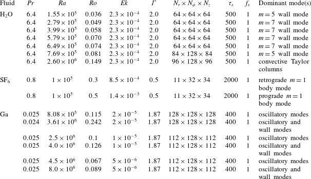
Control parameters
 $Pr$
,
 $Ra$
,
 $Ro$
,
 $Ek$
, and
 $\unicode[STIX]{x1D6E4}$
and the numerical resolution
 $N_{r}\times N_{\unicode[STIX]{x1D719}}\times N_{z}$
used in the DNS, as well as the sampling time
 $\unicode[STIX]{x1D70F}_{s}$
and the sampling frequency
 $f_{s}$
for the DMD. The last column gives the dominant modes, discussed in detail in § 3 for water, in § 4 for sulfur hexafluoride, and in § 5 for gallium.
2.2 Dynamic mode decomposition (DMD) in its sparsity-promoting variant
The dynamic mode decomposition (DMD), developed by Schmid (Reference Schmid2010), is a data-driven technique for the identification and extraction of the dynamically most relevant structures in a flow. The DMD can be considered as a numerical approximation of the Koopman spectral analysis, i.e. it approximates Koopman modes and eigenvalues (Rowley et al. Reference Rowley, Mezić, Bagheri, Schlatter and Henningson2009; Tu et al. Reference Tu, Rowley, Luchtenburg, Brunton and Kutz2014). It is distinctively well suited for oscillating flows, i.e. flows with very specific frequencies, and where various instability mechanisms are present. These properties make it particularly fitting in the analysis of the flow in rotating convection of liquid metals.
Along this line, one of the paramount advantages of DMD is that the extracted dynamic modes (or DMD modes) consist of exactly one frequency. This does not only make their physical interpretation rather straightforward, but it also allows for an easy connection of a flow structure to either numerically or experimentally obtained spectra stemming from point-wise local time series. Moreover, and maybe even more importantly, the DMD algorithm yields information about the temporal evolution, i.e. the dynamics, of these coherent structures.
These attributes clearly distinguish DMD and make it superior to the classical proper orthogonal decomposition (POD) (Sirovich Reference Sirovich1987), also known as principal component analysis: POD modes typically have a multi-frequency content and only provide static information based on their generic energy content. It should, however, be noted that POD modes can be easily recovered as a byproduct of DMD. Another advantage of DMD over POD is that it is not necessary to evaluate an integer number of a typical period (Chen, Tu & Rowley Reference Chen, Tu and Rowley2012) and, unlike POD, does not yield unintended results in this case. Furthermore, in combination with the sparsity-promoting algorithm by Jovanović, Schmid & Nichols (Reference Jovanović, Schmid and Nichols2014), the dynamic modes can be ranked by their dynamical importance, in contrast to POD, where the modes are ranked by their energy content. This is crucial for the understanding of the entire dynamics of the flow, since it is well known that often even low-energetic modes are nonetheless important.
For linearised data, the DMD yields global stability results. For nonlinear data, that shall solely be considered here, the results represent a linear tangent approximation of the flow. It is assumed that temporally successive flow fields, i.e. snapshots
 $\boldsymbol{v}_{k}$
and
 $\boldsymbol{v}_{k+1}$
, are connected by a linear mapping
 $\unicode[STIX]{x1D63C}$
, which does not change over the entire sampling period
 $\unicode[STIX]{x1D70F}_{s}$
, i.e. it holds that
 $\boldsymbol{v}_{k+1}=\unicode[STIX]{x1D63C}\boldsymbol{v}_{k}$
. Thus, the complete flow
 $\unicode[STIX]{x1D651}_{1}^{N}$
can be expressed as a Krylov sequence
 $\{\boldsymbol{v}_{1},\unicode[STIX]{x1D63C}\boldsymbol{v}_{1},\unicode[STIX]{x1D63C}^{2}\boldsymbol{v}_{1},\ldots ,\unicode[STIX]{x1D63C}^{N-1}\boldsymbol{v}_{1}\}$
, where the subscript of
 $\unicode[STIX]{x1D651}$
denotes the index of the first entry of the series and the superscript the last one. A single flow field is, hence, given by
 $\boldsymbol{v}_{k}=\unicode[STIX]{x1D63C}^{k-1}\boldsymbol{v}_{1}$
. By means of DMD an optimal representation of
 $\unicode[STIX]{x1D63C}$
is sought.
The vectors
 $\boldsymbol{v}_{k}$
can be any flow variable, or several. There are no requirements on the geometry, and it is also possible to analyse only a subset of the full numerical (or alternatively experimental) domain.
For the sake of completeness, the basic algorithm to extract dynamic modes (Schmid Reference Schmid2010) is briefly recapitulated here. We will assume that full instantaneous flow fields from the goldfish DNS will be processed; thus, the data are real-valued, and one snapshot is expressed as a column vector
 $\boldsymbol{v}_{k}=(T,u_{r},u_{\unicode[STIX]{x1D719}},u_{z})_{k}$
at a given time
 $t_{k}$
with dimension
 $M=4N_{r}N_{\unicode[STIX]{x1D719}}N_{z}$
.
-
(i) Collect
 $N$
temporally equidistant snapshots
$\{\boldsymbol{v}_{1},\boldsymbol{v}_{2},\boldsymbol{v}_{3},\ldots ,\boldsymbol{v}_{N}\}$
,
$\boldsymbol{v}_{k}\in \mathbb{R}^{M\times 1}$
.
-
(ii) Cast the first
$N-1$
snapshots into a matrix
$\unicode[STIX]{x1D651}_{1}^{N-1}\in \mathbb{R}^{M\times (N-1)}$
, that is (2.6)
$$\begin{eqnarray}\unicode[STIX]{x1D651}_{1}^{N-1}=(\begin{array}{@{}ccccc@{}}\boldsymbol{v}_{1} & \boldsymbol{v}_{2} & \boldsymbol{v}_{3} & \cdots \, & \boldsymbol{v}_{N-1}\end{array}).\end{eqnarray}$$
-
(iii) Perform a singular value decomposition (SVD),
(2.7)The superscript
$$\begin{eqnarray}\unicode[STIX]{x1D651}_{1}^{N-1}=\unicode[STIX]{x1D650}\unicode[STIX]{x1D6F4}\unicode[STIX]{x1D652}^{H}.\end{eqnarray}$$
$H$
denotes the conjugate-transpose of a matrix. The number of non-zero elements in
$\unicode[STIX]{x1D6F4}$
determines the rank
$q$
of
$\unicode[STIX]{x1D651}_{1}^{N-1}$
, thus
$\unicode[STIX]{x1D6F4}\in \mathbb{R}^{q\times q}$
. The matrix
$\unicode[STIX]{x1D650}\in \mathbb{R}^{M\times q}$
contains the spatial structures and
$\unicode[STIX]{x1D652}\in \mathbb{R}^{(N-1)\times q}$
the temporal ones, i.e. the POD modes are given be the
$k$
th column of
$\unicode[STIX]{x1D650}$
. They are ranked by their energy content, i.e. their eigenvalues
$\unicode[STIX]{x1D706}_{k}^{POD}=\unicode[STIX]{x1D6F4}_{kk}^{2}$
.
-
(iv) Combine the last
$N-1$
snapshots,
$\unicode[STIX]{x1D651}_{2}^{N}\in \mathbb{R}^{M\times (N-1)}$
with the matrices
$\unicode[STIX]{x1D650}$
and
$\unicode[STIX]{x1D652}$
and calculate the optimal representation
$\unicode[STIX]{x1D64E}\in \mathbb{R}^{q\times q}$
of the linear mapping
$\unicode[STIX]{x1D63C}$
in the basis spanned by the POD modes, (2.8)
$$\begin{eqnarray}\unicode[STIX]{x1D64E}=\unicode[STIX]{x1D650}^{H}\unicode[STIX]{x1D651}_{2}^{N}\unicode[STIX]{x1D652}\unicode[STIX]{x1D6F4}^{-1}.\end{eqnarray}$$
-
(v) Obtain the eigenvectors
$\unicode[STIX]{x1D654}\in \mathbb{C}^{q\times q}$
and the complex eigenvalues
$\unicode[STIX]{x1D706}_{k}$
of
$\unicode[STIX]{x1D64E}$
, (2.9)
$$\begin{eqnarray}\unicode[STIX]{x1D64E}\boldsymbol{y}_{\boldsymbol{k}}=\unicode[STIX]{x1D706}_{k}\boldsymbol{y}_{\boldsymbol{k}}.\end{eqnarray}$$
-
(vi) Compute the dynamic modes,
$\unicode[STIX]{x1D6F9}\in \mathbb{C}^{M\times q}$
, (2.10)
$$\begin{eqnarray}\unicode[STIX]{x1D74D}_{k}=\unicode[STIX]{x1D650}\boldsymbol{y}_{k}.\end{eqnarray}$$




In matrix form, the full flow
 $\unicode[STIX]{x1D651}_{1}^{N-1}$
can now approximately be expressed as (Jovanović et al.
Reference Jovanović, Schmid and Nichols2014):
 $$\begin{eqnarray}\underbrace{(\boldsymbol{v}_{1}\;\boldsymbol{v}_{2}\;\cdots \;\boldsymbol{v}_{N-1})}_{\unicode[STIX]{x1D651}_{1}^{N-1}}\approx \underbrace{(\unicode[STIX]{x1D74D}_{1}\;\unicode[STIX]{x1D74D}_{2}\;\cdots \;\unicode[STIX]{x1D74D}_{q})}_{\unicode[STIX]{x1D6F9}}\underbrace{\left(\begin{array}{@{}cccc@{}}a_{1} & & & \\ & a_{2} & & \\ & & \ddots & \\ & & & a_{q}\end{array}\right)}_{\unicode[STIX]{x1D63F}_{a}\equiv \operatorname{diag}(a_{k})}\underbrace{\left(\begin{array}{@{}cccc@{}}1 & \unicode[STIX]{x1D706}_{1} & \cdots \, & \unicode[STIX]{x1D706}_{1}^{N-1}\\ 1 & \unicode[STIX]{x1D706}_{2} & \cdots \, & \unicode[STIX]{x1D706}_{2}^{N-1}\\ \vdots & \vdots & \ddots & \vdots \\ 1 & \unicode[STIX]{x1D706}_{q} & \cdots \, & \unicode[STIX]{x1D706}_{q}^{N-1}\\ \end{array}\right)}_{\unicode[STIX]{x1D651}_{and}},\end{eqnarray}$$
where
 $\unicode[STIX]{x1D63F}_{a}$
contains the complex amplitudes, and the Vandermonde matrix
 $\unicode[STIX]{x1D651}_{and}$
is determined by the eigenvalues
 $\unicode[STIX]{x1D706}_{k}$
of
 $\unicode[STIX]{x1D64E}$
. The amplitudes
 $a_{k}$
for the full-rank dynamic modes, i.e. with rank
 $q$
, are given by
 $$\begin{eqnarray}\unicode[STIX]{x1D63F}_{a}=((\unicode[STIX]{x1D654}^{H}\unicode[STIX]{x1D654})\circ \overline{(\unicode[STIX]{x1D651}_{and}\unicode[STIX]{x1D651}_{and}^{H})})^{-1}\;\overline{\operatorname{diag}(\unicode[STIX]{x1D651}_{and}\unicode[STIX]{x1D652}\unicode[STIX]{x1D6F4}^{H}Y)},\end{eqnarray}$$
where the overbar denotes the complex-conjugate of a matrix, and
 $\circ$
the Schur product.
Since the DNS data are real-valued, the eigenvalues appear either in complex-conjugate pairs or are real, i.e. are non-oscillatory. In the latter case, they do not play any role for the dynamics as they are present the entire time. The common logarithmic mapping associates the eigenvalues with the frequency
 $\unicode[STIX]{x1D714}_{k}$
and the decay rate
 $\unicode[STIX]{x1D70E}_{k}$
of the DMD mode, i.e.
 $$\begin{eqnarray}\unicode[STIX]{x1D714}_{k}=\frac{\text{Im}(\ln (\unicode[STIX]{x1D706}_{k}))}{\unicode[STIX]{x0394}t},\quad \unicode[STIX]{x1D70E}_{k}=\frac{\text{Re}(\ln (\unicode[STIX]{x1D706}_{k}))}{\unicode[STIX]{x0394}t},\end{eqnarray}$$
with
 $\unicode[STIX]{x0394}t$
as the time step between the snapshots, i.e. the inverse sampling rate
 $1/f_{s}$
. However, we only consider flow fields obtained from nonlinear simulations; thus, all the eigenvalues are expected to be neutrally stable, i.e. they lie on the unit circle for sufficiently long time series. The reason is that instabilities become nonlinearly saturated and all decaying processes are to disappear.
The approximate flow can herewith be represented by
 $$\begin{eqnarray}\boldsymbol{v}(t)\approx \mathop{\sum }_{k}a_{k}\text{e}^{(\unicode[STIX]{x1D70E}_{k}+\text{i}\unicode[STIX]{x1D714}_{k})t}\unicode[STIX]{x1D74D}_{k}.\end{eqnarray}$$
Naturally, the more DMD modes are included, the more accurate this approximation becomes.
The sparsity-promoting algorithm by Jovanović et al. (Reference Jovanović, Schmid and Nichols2014) allows one to further fix a desired number of snapshots by still optimally approximating the flow, or to fix the quality of approximation retaining a minimal number of modes. The best tradeoff between both approaches depends on the respective objective of the considered problem. The crucial point in the sparsity-promoting variant of DMD is to determine the amplitudes of the reduced system, i.e. the respective sparse DMD modes. This amounts to solving the optimisation problem
 $$\begin{eqnarray}\underset{\boldsymbol{a}}{\text{minimise}}\;J(\boldsymbol{a})\equiv \Vert \unicode[STIX]{x1D6F4}\unicode[STIX]{x1D652}^{H}-\unicode[STIX]{x1D654}\unicode[STIX]{x1D63F}_{a}\unicode[STIX]{x1D651}_{and}\Vert _{F}^{2},\end{eqnarray}$$
where the subscript
 $F$
indicates the Frobenius norm. Instead of solving (2.15), sparsity promotion means to solve the optimisation problem by penalising the number of non-zero elements in the unknown vector
 $(a_{k})$
. Using the
 $l_{1}$
-norm as a relaxed version of the cardinality of
 $(a_{k})$
, we thus calculate
 $$\begin{eqnarray}\underset{\boldsymbol{a}}{\text{minimise}}\;J(\boldsymbol{a})+\unicode[STIX]{x1D701}\mathop{\sum }_{k}|a_{k}|,\end{eqnarray}$$
with the sparsity-promoting parameter
 $\unicode[STIX]{x1D701}$
. The quality of the sparse approximation can be judged using the performance loss
 $$\begin{eqnarray}\%\unicode[STIX]{x1D6F1}_{loss}=100\sqrt{\frac{J(\boldsymbol{a})}{J(0)}}=\frac{\Vert \unicode[STIX]{x1D651}_{1}^{N-1}-\unicode[STIX]{x1D6F9}\unicode[STIX]{x1D63F}_{\unicode[STIX]{x1D6FC}}\unicode[STIX]{x1D651}_{and}\Vert _{F}}{\Vert \unicode[STIX]{x1D651}_{1}^{N-1}\Vert _{F}}.\end{eqnarray}$$
Employing the sparsity-promoting variant of DMD also implies that we are able to select and rank the DMD modes based on their importance to the total dynamics of the system.
3 Wall modes and stationary modes in rotating convection of water
First, we apply the DMD to rotating RBC of water with
 $Pr=6.4$
,
 $Ek=2.331\times 10^{-4}$
,
 $\unicode[STIX]{x1D6E4}=2$
and varying
 $Ra;$
the exact parameters are given in table 1. All DNS were performed relatively close to the onset of convection, where linear stability analysis (Goldstein et al.
Reference Goldstein, Knobloch, Mercader and Net1993) and experimental data (Zhong et al.
Reference Zhong, Ecke and Steinberg1991; Ecke et al.
Reference Ecke, Zhong and Knobloch1992; Ning & Ecke Reference Ning and Ecke1993; Zhong et al.
Reference Zhong, Ecke and Steinberg1993) are available. This makes it an appealing validation example and an ideal case to prove the applicability of DMD to identify the dominant modes and their frequencies.
The numerical simulations are carried out in cylindrical tanks, where the conductive state initially becomes unstable through a Hopf bifurcation leading to precessing wall modes. The instabilities in this case are induced, as the name suggests, by the lateral walls. In the limit of
 $Ek\rightarrow 0$
and neglecting the curvature of the cylinder, the critical Rayleigh number is given by
 $$\begin{eqnarray}Ra_{w}=\unicode[STIX]{x03C0}^{2}(6\sqrt{3})^{1/2}Ek^{-1}+46.55Ek^{-2/3},\end{eqnarray}$$
with an onset frequency (Zhang & Liao Reference Zhang and Liao2009) of
 $$\begin{eqnarray}\widetilde{\unicode[STIX]{x1D714}}_{w}=(2\unicode[STIX]{x03C0})^{2}\sqrt{3}(2+\sqrt{3})^{1/2}\frac{Ek}{Pr}-1464.53\frac{Ek^{4/3}}{Pr}.\end{eqnarray}$$
The frequency
 $\widetilde{\unicode[STIX]{x1D714}}_{w}$
is normalised with the system’s rotation rate
 $\unicode[STIX]{x1D6FA}$
. The system’s rotation time scale is
 $1/(2\unicode[STIX]{x1D6FA})$
. Equations (3.1) and (3.2) are in agreement with the results by Herrmann & Busse (Reference Herrmann and Busse1993), but provide a higher-order correction to account for the no-slip boundary conditions at the top and bottom.
The onset in a confined container and for
 $Pr>0.68$
is always at a lower Rayleigh number than the predicted stationary onset in an infinite layer. There the critical Rayleigh number in the asymptotic limit of rapid rotation and for isothermal top and bottom boundary conditions (Chandrasekhar Reference Chandrasekhar1961) is given by
 $$\begin{eqnarray}Ra_{s}^{\infty }={\textstyle \frac{3}{2}}(2\unicode[STIX]{x03C0}^{4})^{1/3}Ek^{-4/3}.\end{eqnarray}$$
The result is asymptotically indistinguishable for no-slip and free-slip boundaries (Clune & Knobloch Reference Clune and Knobloch1993). Notably, both critical Rayleigh numbers,
 $Ra_{w}$
and
 $Ra_{s}^{\infty }$
, are independent of
 $Pr$
. For the parameters considered here, this gives
 $Ra_{w}=1.49\times 10^{5}$
,
 $\widetilde{\unicode[STIX]{x1D714}}_{w}=1.53\times 10^{-3}$
, and
 $Ra_{s}^{\infty }=6.06\times 10^{5}$
. However, the Ekman number is not sufficiently low yet for the asymptotic solution to be very accurate (see also § 5). Thus, we compare to the experimental value for the onset frequency obtained by Zhong et al. (Reference Zhong, Ecke and Steinberg1993), with
 $\widetilde{\unicode[STIX]{x1D714}}_{0}^{exp}=3.04\times 10^{-3}$
.
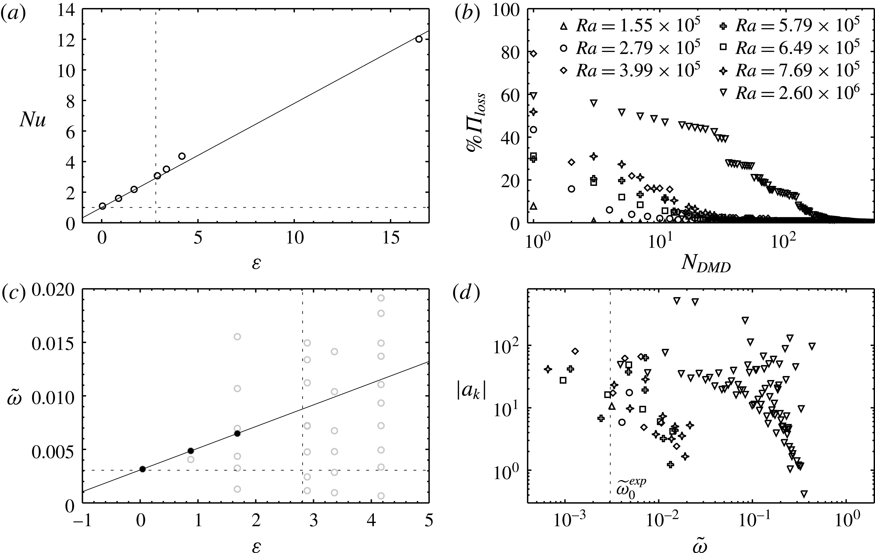
(a) Nusselt number versus the reduced bifurcation parameter
 $\unicode[STIX]{x1D700}=(Ra-Ra_{w})/Ra_{w}$
for
 $Pr=6.4$
,
 $\unicode[STIX]{x1D6E4}=2$
,
 $Ek=2.33\times 10^{-4}$
. The dashed horizontal line corresponds to the purely conducting state with
 $Nu=1$
, the solid line to a linear scaling of
 $Nu$
with
 $\unicode[STIX]{x1D700}$
, and the dashed vertical line corresponds to the transition
 $\unicode[STIX]{x1D700}\approx 2.8$
obtained experimentally by Zhong et al. (Reference Zhong, Ecke and Steinberg1993). (b) Performance loss as a function of the number of retained DMD modes. (c) Frequencies obtained from DMD. For all cases
 $\unicode[STIX]{x1D6F1}_{loss}$
was fixed to
 $5\,\%$
. The dashed horizontal line shows the experimental onset frequency
 $\widetilde{\unicode[STIX]{x1D714}}_{0}^{exp}=3.04\times 10^{-3}$
, and the dashed vertical line corresponds to the transition
 $\unicode[STIX]{x1D700}\approx 2.8$
obtained experimentally by Zhong et al. (Reference Zhong, Ecke and Steinberg1993). The filled symbols indicate pure wall modes, and the solid line shows a linear fit through them. (d) Absolute values of the DMD amplitudes versus normalised frequencies of the dominant modes guaranteeing a maximum performance loss of
 $\unicode[STIX]{x1D6F1}_{loss}\leqslant 10\,\%$
. The dashed vertical line indicates
 $\widetilde{\unicode[STIX]{x1D714}}_{0}^{exp}$
. The symbols are the same as in (b).

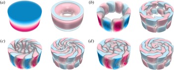
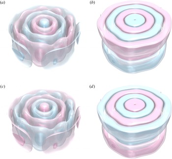
Isosurfaces of the real part of the temperature
 $T$
and the azimuthal velocity
 $u_{\unicode[STIX]{x1D719}}$
of the DMD modes for
 $Pr=6.4$
, corresponding to water,
 $\unicode[STIX]{x1D6E4}=2$
,
 $Ek=2.33\times 10^{-4}$
. In each case
 $T$
is visualised on the left,
 $u_{\unicode[STIX]{x1D719}}$
on the right. The isosurfaces are equidistantly distributed between
 $[T_{t},T_{b}]$
and
 $[-\text{max}\,|u_{\unicode[STIX]{x1D719}}|,\text{max}\,|u_{\unicode[STIX]{x1D719}}|]$
, respectively. (a)
 $Ra=1.55\times 10^{5}$
,
 $m=0$
mode; (b)
 $Ra=1.55\times 10^{5}$
, dominant
 $m=5$
wall mode; (c)
 $Ra=6.49\times 10^{5}$
, mixed
 $m=7$
mode; (d)
 $Ra=7.69\times 10^{5}$
, mixed
 $m=5$
mode. See also the supplementary movies 1, 2 and 3 (available at https://doi.org/10.1017/jfm.2017.631) for the full DNS.

In figure 1(a), the dimensionless heat flux, expressed in terms of the Nusselt number
 $Nu\equiv Pr^{1/2}Ra^{1/2}\unicode[STIX]{x1D6FE}^{1/2}u_{z}T-\unicode[STIX]{x1D6FE}^{-1}\unicode[STIX]{x2202}_{z}T$
, and evaluated as an average over all horizontal planes, is presented as a function of the reduced bifurcation parameter
 $\unicode[STIX]{x1D700}(Ra)=(Ra-Ra_{w})/Ra_{w}$
introduced by Ecke et al. (Reference Ecke, Zhong and Knobloch1992), Zhong et al. (Reference Zhong, Ecke and Steinberg1993). For
 $\unicode[STIX]{x1D700}\lesssim 2.9$
,
 $Nu$
approximately follows a linear scaling, which was also found experimentally by Zhong et al. (Reference Zhong, Ecke and Steinberg1993), who reported a transition at
 $\unicode[STIX]{x1D700}\approx 2.8$
. This value is consistent with
 $\unicode[STIX]{x1D700}(Ra_{s})=3.1$
, considering the asymptotic nature of
 $Ra_{s}$
and
 $Ra_{w}$
, and the fact that both are derived for infinite and half-infinite fluid layers, respectively. After the steady-state onset the slope of
 $Nu$
with respect to
 $Ra$
first increases and ultimately becomes less steep.
With DMD we can further elucidate this transition. We extracted the dynamic modes for a time period of
 $500$
time units with a sampling period of
 $f_{s}=1$
. As to be expected, more modes need to be retained for increasing
 $Ra$
to still guarantee an accurate representation of the flow, as shown in figure 1(b). The most dominant mode corresponds to a base or mean flow, as visualised in figure 2(a) for
 $Ra=1.55\times 10^{5}$
and
 $\unicode[STIX]{x1D700}=0.04$
, which resembles the conductive state, while the azimuthal flow shows a mainly constant retrograde flow, and a prograde corner flow, which is a Stewartson extension of the Ekman layer (Kunnen, Clercx & van Heijst Reference Kunnen, Clercx and van Heijst2013). However, this flow is evidently dynamically not important. The principal DMD mode is a wall-localised mode with an azimuthal wavenumber of
 $m=5$
, shown in figure 2(b). This is in agreement with the onset mode predicted by Goldstein et al. (Reference Goldstein, Knobloch, Mercader and Net1993) and experimentally found by Zhong et al. (Reference Zhong, Ecke and Steinberg1993). For increasing
 $Ra$
, at
 $Ra=2.79\times 10^{5}$
and
 $\unicode[STIX]{x1D700}=0.88$
, the flow is still essentially described by a single wall mode, although with
 $m=7$
. All other modes are higher-order Fourier components (Chen et al.
Reference Chen, Tu and Rowley2012). For
 $Ra=3.99\times 10^{5}$
and
 $\unicode[STIX]{x1D700}=1.68$
, the dominant mode is no longer purely wall-localised, but faint columnar vortices appear in the centre. Nonetheless, the second most important mode is still a clean
 $m=7$
wall mode. The frequencies of these modes have a linear dependence on
 $\unicode[STIX]{x1D700}$
, i.e.
 $\widetilde{\unicode[STIX]{x1D714}}\propto \unicode[STIX]{x1D700}$
, as expected for a Hopf bifurcation. A linear fit yields an onset frequency of
 $\widetilde{\unicode[STIX]{x1D714}}_{0}^{DMD}=3.08$
which is in respectable agreement with
 $\widetilde{\unicode[STIX]{x1D714}}_{0}^{exp}$
, as shown in figure 1(c). The linear behaviour does not hold for larger
 $\unicode[STIX]{x1D700}$
, i.e. even higher
 $Ra$
. Then, all dynamic modes are mixed modes, i.e. they are nonlinear superpositions of wall modes and body modes, as exemplary shown for
 $Ra=6.49\times 10^{5}$
and
 $\unicode[STIX]{x1D700}=3.36$
in figure 2(c). The inner bulk modes are associated with the stationary onset of convection, as discussed in the introduction, and they are modulated by the wall modes. For
 $Ra=7.69\times 10^{5}$
and
 $\unicode[STIX]{x1D700}=4.17$
, presented in figure 2(d), the bulk contribution and the wall-mode contribution are of comparable strength. Remarkably, the dominant mode is again an
 $m=5$
wall mode. That the DMD does not decompose the wall modes and the bulk modes is well substantiated by the fact that wall modes are indeed not restricted to the near-wall region but are actually filling the entire convection cell, albeit with decreasing magnitude from the sidewall to the centre. Thus, their motion also affects the bulk modes, and they precess with the same frequency. For increasing
 $Ra$
, the interior modes dominate over the wall modes.
Ultimately, the flow becomes dominated by convective Taylor columns, as shown in movie 3. At
 $Ra=2.60\times 10^{6}$
,
 $\unicode[STIX]{x1D700}=16.47$
there are no longer modes present with a pronounced wall localisation, and a multitude of dynamic modes is necessary to accurately describe the flow. This can also be seen in the DMD spectra in figure 1(d). For
 $Ra\lesssim 7.69\times 10^{5}$
there are only few retained modes with low frequencies, while for
 $Ra=2.60\times 10^{6}$
, most modes are almost exclusively at higher frequencies and, in addition, span a rather broad range.
4 Identification of retrograde and prograde precession in
$\text{SF}_{6}$

For moderate Prandtl numbers and relatively large aspect ratios, as in the example discussed in the previous § 3, it is clear that the precession direction of the dominant modes is retrograde. However, theory (Goldstein et al. Reference Goldstein, Knobloch, Mercader and Net1993, Reference Goldstein, Knobloch, Mercader and Net1994) predicts that this is no longer the case for small Prandtl numbers or aspect ratios. Unfortunately, information about the precession direction is not directly evident from the extracted DMD frequencies, because real-valued data are processed. Hence, the DMD eigenvalues appear in complex-conjugate pairs, and there is always a corresponding positive frequency to a negative one.
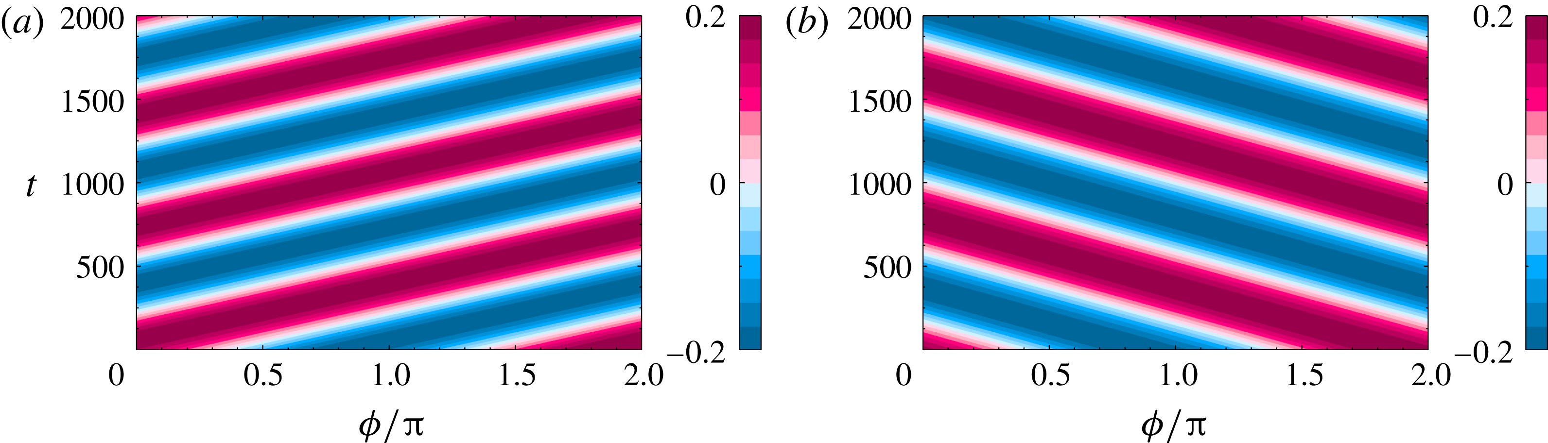
Space-time diagrams of the temperature
 $T$
at the sidewall,
 $r=R$
and half-height,
 $z=H/2$
for
 $Pr=0.8$
,
 $Ra=10^{5}$
,
 $\unicode[STIX]{x1D6E4}=0.5$
, and (a)
 $Ro=0.3$
: retrograde, (b)
 $Ro=0.5$
: prograde. See also the supplementary movie 4.

One way of identifying the direction of travel is to develop the modes in time according to (2.14). Yet, this method can get cumbersome for a larger number of modes, even though confirming that the precession direction is immanent in the formulation of the DMD modes.
Here, we will present an alternative identification criterion exemplified on a fluid with
 $Pr=0.8$
, corresponding to SF
 $_{6}$
, in a slender cylinder with
 $\unicode[STIX]{x1D6E4}=1/2$
and at
 $Ra=10^{5}$
. This set-up constitutes a very illustrative example, because it displays a topologically simple
 $m=1$
mode that, depending on the rotation rate, either precesses prograde or retrograde (Horn & Shishkina Reference Horn and Shishkina2015). More precisely, at
 $Ro=0.3$
the precession is prograde, and at
 $Ro=0.5$
the precession is retrograde, as can clearly be seen in figure 3 and in movie 4. Furthermore, there is no precession for
 $Ro=0.367$
. It is worth noting that prograde modes are not restricted to low
 $Pr$
, but have also been found in water with
 $Pr=4.38$
for
 $\unicode[STIX]{x1D6E4}=0.5$
by Weiss & Ahlers (Reference Weiss and Ahlers2011b
). They are likely related to the prograde precessing body modes discussed by Goldstein et al. (Reference Goldstein, Knobloch, Mercader and Net1993).
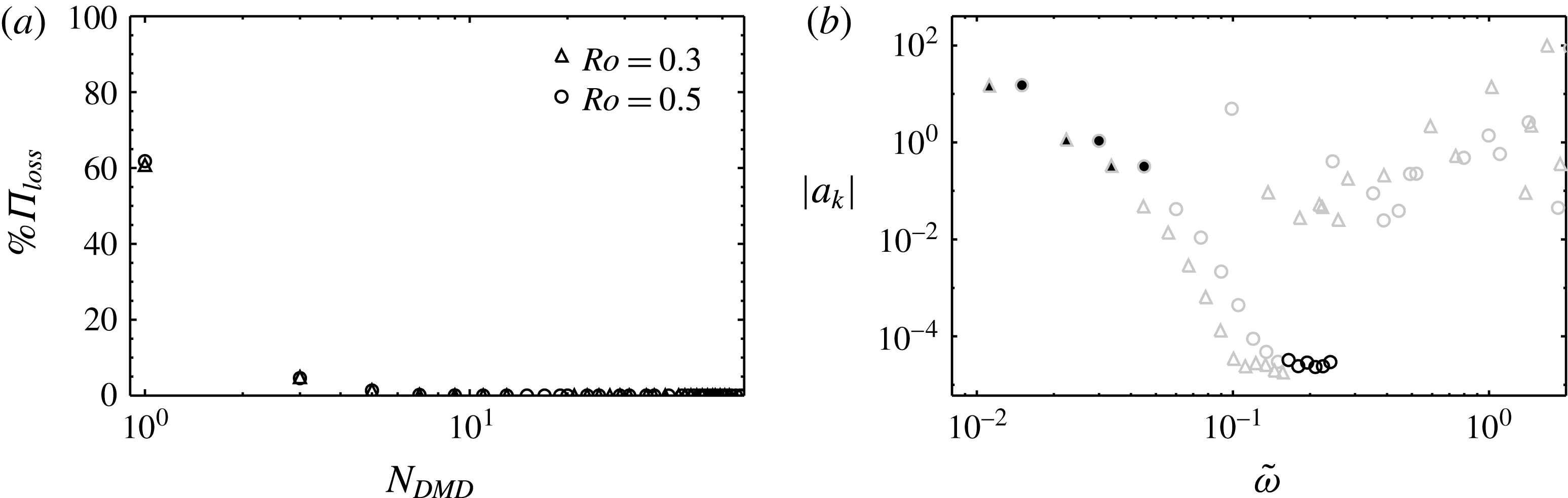
Due to the relatively simple flow, the sparsity-promoting DMD algorithm retains only three dynamic modes to already guarantee a loss rate of less than
 $\%\unicode[STIX]{x1D6F1}_{loss}=1\,\%$
, and the amplitudes of the modes all lie on the same branch, see figure 4. Owing to the fact that there is only one travelling periodic wave, the first nine modes in either case can be interpreted as Fourier components belonging to the same structure (Chen et al.
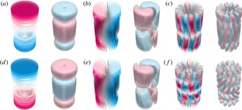
Reference Chen, Tu and Rowley2012). This is also supported by the spatial structures visualised by the real part of the temperature and the azimuthal velocity in figure 5. The zeroth modes are presented in figures 5(a) and 5(d) and are the modes with zero frequency. They do not, formally, contribute to the dynamics of the flow; nonetheless, they are instructive. They indicate not only that the bulk flow is retrograde for
 $Ro=0.3$
and prograde for
 $Ro=0.5$
, but also that the mean temperature gradient is destabilising for
 $Ro=0.3$
and, remarkably, stabilising for
 $Ro=0.5$
. The most dominant
 $m=1$
modes, shown in figures 5(b) and 5(e), are visually indistinguishable and provide no hint on the precession direction. The higher
 $m=6$
modes, displayed in figures 5(c) and 5(f), show that the vertical structure is in fact different for
 $Ro=0.3$
and
 $Ro=0.5$
, but because of their low amplitudes they only exert an insignificant influence on the actual flow.
(a) Performance loss
 $\%\unicode[STIX]{x1D6F1}_{loss}$
as a function of the number of retained DMD modes
 $N_{DMD}$
for
 $Pr=0.8$
,
 $Ra=10^{5}$
,
 $\unicode[STIX]{x1D6E4}=0.5$
. Triangles mark
 $Ro=0.3$
and circles mark
 $Ro=0.5$
. (b) Entire spectrum, i.e. amplitudes
 $|a_{k}|$
versus frequency
 $\widetilde{\unicode[STIX]{x1D714}}$
, shown with grey open symbols. The amplitudes corresponding to a loss rate of
 $\unicode[STIX]{x1D6F1}_{loss}=1\,\%$
are demarcated by closed black symbols. Triangles mark
 $Ro=0.3$
and circles mark
 $Ro=0.5$
. In addition, we indicate the oscillating modes for
 $Ro=0.5$
with black open circles.

Isosurfaces of the real part of the temperature
 $T$
and the azimuthal velocity
 $u_{\unicode[STIX]{x1D719}}$
of the DMD modes for
 $Pr=0.8$
, corresponding to
 $\text{SF}_{6}$
,
 $Ra=10^{5}$
, and
 $\unicode[STIX]{x1D6E4}=0.5$
. (a–c) Show the modes for
 $Ro=0.3$
, and (d–f) show the modes for
 $Ro=0.5$
, with the azimuthal wavenumbers (a), (d)
 $m=0$
; (b), (e)
 $m=1$
; and (c), (f)
 $m=6$
. In each case
 $T$
is visualised on the left,
 $u_{\unicode[STIX]{x1D719}}$
on the right.

To develop a criterion for the precession direction, we start with (2.14), which describes the approximate flow as a superposition of all modes, and only look at the temporal evolution of the
 $k$
th mode. Since we consider a nonlinear problem, we can further assume that the decay rate is negligible; a single mode can then be expressed as
 $$\begin{eqnarray}\displaystyle \unicode[STIX]{x1D6F9}_{k} & = & \displaystyle a_{k}\unicode[STIX]{x1D74D}_{k}\exp (\text{i}\unicode[STIX]{x1D714}_{k}t)\end{eqnarray}$$
 $$\begin{eqnarray}\displaystyle & = & \displaystyle |a_{k}|\exp (\text{i}\operatorname{Arg}(a_{k}))|\unicode[STIX]{x1D74D}_{k}|\exp (\text{i}\operatorname{Arg}(\unicode[STIX]{x1D74D}_{k}))\exp (\text{i}\unicode[STIX]{x1D714}_{k}t).\end{eqnarray}$$
Here,
 $a_{k}$
and
 $\unicode[STIX]{x1D74D}_{k}$
are represented by their complex modulus and argument. The argument for any complex number
 $z=x+\text{i}y$
is given by
 $\operatorname{Arg}(z)=\text{atan2}(y,x)$
and defined in the principal interval
 $(-\unicode[STIX]{x03C0},\unicode[STIX]{x03C0}]$
. In the following, we will only focus on the physical real part
 $\text{Re}(\unicode[STIX]{x1D6F9}_{k})$
, although the analogous argumentation can be made for the imaginary part
 $\text{Im}(\unicode[STIX]{x1D6F9}_{k})$
. Both exhibit the same precession direction. We have
 $$\begin{eqnarray}\text{Re}(\unicode[STIX]{x1D6F9}_{k})=|a_{k}||\unicode[STIX]{x1D74D}_{k}|\cos (\unicode[STIX]{x1D714}_{k}t+\operatorname{Arg}(\unicode[STIX]{x1D74D}_{k})+\operatorname{Arg}(a_{k})),\end{eqnarray}$$
which can be interpreted as a standard travelling-wave equation.
 $\operatorname{Arg}(a_{k})$
is a constant and, hence, merely represents a phase shift
 $\unicode[STIX]{x1D703}$
. Therefore, it is generally the phase between the real part and the imaginary part of the DMD mode that determines the direction of travel.
We can make further assumptions for the azimuthally travelling waves in rotating Rayleigh–Bénard convection. First, we separate
 $\unicode[STIX]{x1D74D}_{k}$
into functions of
 $r$
and
 $z$
, and
 $\unicode[STIX]{x1D719}$
, i.e.
 $\unicode[STIX]{x1D713}=f(r,z)g(\unicode[STIX]{x1D719})$
. Note that in our case, typically,
 $\text{Re}(f(r,z))\approx \text{Im}(f(r,z))$
, and both are time independent. Secondly, the waves are known to be travelling in the azimuthal direction, consequently
 $\operatorname{Arg}(g(\unicode[STIX]{x1D719}))$
is required to be a linear function of
 $\unicode[STIX]{x1D719}$
, and (4.3) can be written as
 $$\begin{eqnarray}\text{Re}(\unicode[STIX]{x1D6F9}_{k})=|a_{k}||\unicode[STIX]{x1D74D}_{k}|\cos (\unicode[STIX]{x1D714}_{k}t+\unicode[STIX]{x1D719}\unicode[STIX]{x2202}_{\unicode[STIX]{x1D719}}\operatorname{Arg}(g(\unicode[STIX]{x1D719}))+\operatorname{Arg}(f(r,z))+\unicode[STIX]{x1D703}).\end{eqnarray}$$
Accordingly,
 $\unicode[STIX]{x2202}_{\unicode[STIX]{x1D719}}\operatorname{Arg}(g(\unicode[STIX]{x1D719}))$
corresponds to a wavenumber, and if
 $\unicode[STIX]{x1D714}_{k}\unicode[STIX]{x2202}_{\unicode[STIX]{x1D719}}\operatorname{Arg}(g(\unicode[STIX]{x1D719}))>0$
, the mode precesses retrograde; conversely, if
 $\unicode[STIX]{x1D714}_{k}\unicode[STIX]{x2202}_{\unicode[STIX]{x1D719}}\operatorname{Arg}(g(\unicode[STIX]{x1D719}))<0$
, the mode precesses prograde.
Cross-section at half-height,
 $z=H/2$
, of the dominant dynamic mode with contours between
 $[-\text{max}\,|\unicode[STIX]{x1D713}(T)|,\text{max}\,|\unicode[STIX]{x1D713}(T)]$
, the left map shows the real part of the temperature,
 $\text{Re}(\unicode[STIX]{x1D713}(T))$
, the right map shows the imaginary part of the temperature,
 $\text{Im}(\unicode[STIX]{x1D713}(T))$
; (a), (b) for the retrograde mode for
 $Ro=0.3$
, with (a) positive and (b) negative DMD frequency associated with it; (c), (d) the prograde mode for
 $Ro=0.5$
with (c) positive and (d) negative frequency, respectively.

We will demonstrate this criterion on the dominant dynamic mode pairs for the prograde and retrograde case in
 $\text{SF}_{6}$
, visualised by their temperature in figure 6. In figure 6(a), we can already visually infer that there is a phase of
 $-\unicode[STIX]{x03C0}/2$
between the real and the imaginary part; in combination with the positive DMD frequency, this means the mode is retrograde. In more detail, we can describe the mode in figure 6(a) by
 $\text{Re}(\unicode[STIX]{x1D713})\propto \cos (\unicode[STIX]{x1D719})$
and
 $\text{Im}(\unicode[STIX]{x1D713})\propto \cos (\unicode[STIX]{x1D719}-\unicode[STIX]{x03C0}/2)$
. From this it follows that
 $\operatorname{Arg}(g)\approx \text{atan2}(\cos (\unicode[STIX]{x1D719}-\unicode[STIX]{x03C0}/2)/\cos (\unicode[STIX]{x1D719}))=\text{atan2}(\sin (\unicode[STIX]{x1D719})/\cos (\unicode[STIX]{x1D719}))=\text{atan2}(\tan (\unicode[STIX]{x1D719}))=\unicode[STIX]{x1D719}$
, which means
 $m=\unicode[STIX]{x2202}_{\unicode[STIX]{x1D719}}\unicode[STIX]{x1D719}=+1$
. Similarly, in figure 6(b), the phase is
 $\unicode[STIX]{x03C0}/2$
and the DMD frequency is negative, or equivalently
 $\operatorname{Arg}(g)\approx \text{atan2}(\cos (\unicode[STIX]{x1D719}+\unicode[STIX]{x03C0}/2)/\cos (\unicode[STIX]{x1D719}))=\text{atan2}(-\sin (\unicode[STIX]{x1D719})/\cos (\unicode[STIX]{x1D719}))=-\unicode[STIX]{x1D719}$
, which means
 $m=-1$
. Hence, also this mode is retrograde, as it must be, since it is just the complex-conjugate twin to the mode shown in figure 6(a). In an analogous way, we can conclude that the modes presented in figure 6(c) and 6(d) are both prograde.
Besides these ordinary precessing waves, we have also found oscillating
 $m=1$
modes. These are indicated by open circles for
 $Ro=0.5$
in figure 4 and are shown in movie 5. Despite the fact that they only have an amplitude of
 $|a_{k}|\approx 10^{-5}$
, making them inconsequential for the overall dynamics of the flow, they are fascinating since oscillating convection is a phenomenon associated only with rotating convection of small-
 $Pr$
fluids, and often the classical result for an infinite layer by Chandrasekhar (Reference Chandrasekhar1961) is invoked stating that it can only occur for
 $Pr\leqslant 0.68$
. However, as mentioned by Goldstein et al. (Reference Goldstein, Knobloch, Mercader and Net1994), for a confined container the upper bound for oscillatory convection is
 $Pr=1$
. We have verified that they are not a numerical artefact caused by insufficient resolution by conducting the DNS on a finer mesh with
 $N_{r}\times N_{\unicode[STIX]{x1D719}}\times N_{z}=20\times 38\times 48$
volume cells which yielded the same result. Furthermore, we confirmed that the eigenvalues associated with these modes lie on the unit circle, i.e. they are not just transients. Consequently, we believe that these are real oscillatory modes, which makes this a quite striking finding.
5 Oscillatory modes and wall modes in liquid gallium
Utilising the results from the previous §§3 and 4, we are now equipped with the tools to address the more complex flows in liquid metals. Here we will focus on a fluid with
 $Pr=0.025$
, corresponding to liquid gallium or mercury, in a cylindrical container with an aspect ratio of
 $\unicode[STIX]{x1D6E4}=1.87$
. The exact parameters for all performed DNS are given in table 1.
5.1 Onset, oscillatory convection and wall modes in low-
$Pr$
fluids

The onset of convection for small Prandtl numbers can occur in a different manner than in higher-
 $Pr$
fluids discussed in § 3, namely in the form of oscillating convection. For
 $Pr\leqslant 0.68$
the critical Rayleigh number in an infinite layer and in the asymptotic limit of rapid rotation is then given by
 $$\begin{eqnarray}Ra_{o}^{\infty }=\frac{3}{2}\frac{(2\unicode[STIX]{x03C0}Pr)^{4/3}}{(1+Pr)^{1/3}}Ek^{-4/3},\end{eqnarray}$$
with an onset oscillation frequency of
 $$\begin{eqnarray}\widetilde{\unicode[STIX]{x1D714}}_{o}^{\infty }=(2\unicode[STIX]{x03C0})^{2/3}\frac{(2-3Pr^{2})^{1/2}}{Pr^{1/3}(1+Pr)^{2/3}}Ek^{1/3},\end{eqnarray}$$
which is again independent of the velocity boundary conditions (Chandrasekhar Reference Chandrasekhar1961; Clune & Knobloch Reference Clune and Knobloch1993). Zhang & Liao (Reference Zhang and Liao2009) developed an asymptotic theory for low Prandtl numbers, rapid rotation rates and accounting for the cylindrical confinement. Based on the assumption that the onset is in the form of large-scale convection-driven inertial oscillatory waves, for brevity, we will refer to them as oscillatory modes, the critical Rayleigh number can herewith be obtained by minimising
 $$\begin{eqnarray}\displaystyle Ra_{o}^{a} & = & \displaystyle \left[\frac{\displaystyle (m^{2}+\unicode[STIX]{x03C0}^{2}\unicode[STIX]{x1D6FE}^{2})\left(\frac{|\unicode[STIX]{x1D70E}_{0}|^{1/2}}{\unicode[STIX]{x1D6FE}}(1-\unicode[STIX]{x1D70E}_{0}^{2})^{1/2}+(1+\unicode[STIX]{x1D70E}_{0})^{3/2}+(1-\unicode[STIX]{x1D70E}_{0})^{3/2}\right)}{4m^{2}(2(1-\unicode[STIX]{x1D70E}_{0}^{2})Ek)^{1/2}}+\frac{\unicode[STIX]{x03C0}^{4}\unicode[STIX]{x1D6FE}^{2}+m\unicode[STIX]{x03C0}^{2}(m-\unicode[STIX]{x1D70E}_{0})}{4m^{2}\unicode[STIX]{x1D70E}_{0}^{2}(1-\unicode[STIX]{x1D70E}_{0}^{2})}\right.\nonumber\\ \displaystyle & & \displaystyle \left.-\,\frac{\unicode[STIX]{x1D70E}_{0}((1+\unicode[STIX]{x1D70E}_{0})^{1/2}+(1-\unicode[STIX]{x1D70E}_{0})^{1/2})}{2m(2(1-\unicode[STIX]{x1D70E}_{0}^{2})Ek)^{1/2}}\right]\left(\mathop{\sum }_{n=1}^{N}\frac{\displaystyle \left(\unicode[STIX]{x03C0}^{2}+\frac{\unicode[STIX]{x1D6FD}_{mn}^{2}}{\unicode[STIX]{x1D6FE}^{2}}\right)Q_{mn}}{\displaystyle \left(\unicode[STIX]{x03C0}^{2}+\frac{\unicode[STIX]{x1D6FD}_{mn}^{2}}{\unicode[STIX]{x1D6FE}^{2}}\right)^{2}+\left(\frac{\unicode[STIX]{x1D70E}_{0}Pr}{Ek}\right)^{2}}\right)^{-1}\end{eqnarray}$$
over
 $m$
and
 $l$
. Here
 $\unicode[STIX]{x1D70E}_{0}$
is a solution for different
 $m$
and
 $l$
of
 $$\begin{eqnarray}\unicode[STIX]{x1D709}\text{J}_{m-1}(\unicode[STIX]{x1D709})+\frac{\unicode[STIX]{x1D70E}_{0}}{|\unicode[STIX]{x1D70E}_{0}|}\left(\sqrt{1+\left(\frac{\unicode[STIX]{x1D709}}{\unicode[STIX]{x1D6FE}\unicode[STIX]{x03C0}}\right)^{2}}-1\right)m\text{J}_{m}(\unicode[STIX]{x1D709})=0,\quad \unicode[STIX]{x1D709}=\unicode[STIX]{x1D6FE}\unicode[STIX]{x03C0}\sqrt{\left(\frac{1}{\unicode[STIX]{x1D70E}_{0}^{2}}-1\right)},\quad\end{eqnarray}$$
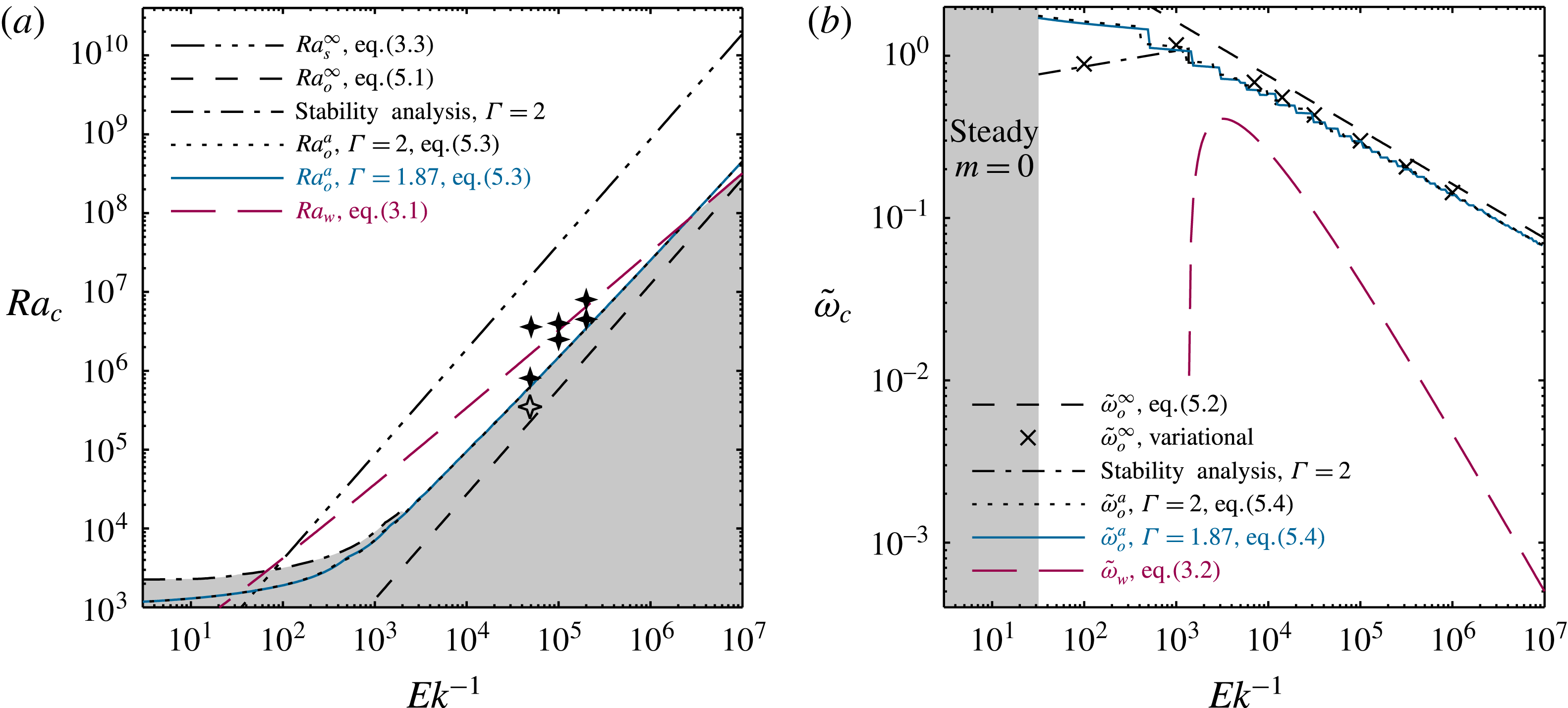
(a) Critical Rayleigh number for the onset of rotating convection in a
 $Pr=0.025$
fluid. Predictions are shown for the stationary and oscillatory onset in an infinite layer,
 $Ra_{s}^{\infty }$
(dashed-triple-dotted line), and
 $Ra_{o}^{\infty }$
(short-dashed line), by Chandrasekhar (Reference Chandrasekhar1961); for the onset in a cylinder with
 $\unicode[STIX]{x1D6E4}=2$
as obtained by the numerical stability analysis by Goldstein et al. (Reference Goldstein, Knobloch, Mercader and Net1994) (dashed-dotted line); for the onset of convection-driven oscillatory inertial waves,
 $Ra_{o}^{a}$
, derived by asymptotics for a
 $\unicode[STIX]{x1D6E4}=2$
(dotted line) and a
 $\unicode[STIX]{x1D6E4}=1.87$
(solid line) cylinder, respectively, and for the onset of wall modes,
 $Ra_{w}$
, (long-dashed line) by Zhang & Liao (Reference Zhang and Liao2009). The stars mark our simulations, and the grey shaded area indicates the parameter region where convection is precluded. (b) Corresponding predictions for the onset frequencies. In addition, results obtained via a variational principle for the infinite layer are marked by crosses (Chandrasekhar Reference Chandrasekhar1961). For
 $\unicode[STIX]{x1D6E4}=2$
,
 $Pr=0.025$
, the preferred onset mode for
 $Ek>3.125\times 10^{-2}$
is a steady
 $m=0$
mode, indicated by the grey shaded area (Goldstein et al.
Reference Goldstein, Knobloch, Mercader and Net1994).

where
 $\text{J}_{m}$
denotes Bessel functions of the first kind,
 $\unicode[STIX]{x1D6FD}_{mn}$
are the roots of their derivatives, and
 $Q_{mn}=(\unicode[STIX]{x03C0}\unicode[STIX]{x1D6FE}\unicode[STIX]{x1D6FD}_{mn})^{2}/[2\unicode[STIX]{x1D70E}_{0}^{2}(\unicode[STIX]{x1D709}^{2}-\unicode[STIX]{x1D6FD}_{mn}^{2})^{2}(\unicode[STIX]{x1D6FD}_{mn}^{2}-m^{2})]$
. Equation (5.3) also yields the structure, i.e. the azimuthal wavenumber
 $m_{c}$
and the number of nodes
 $l_{c}$
in the radial direction, for the onset mode. The onset frequency is given similarly by
 $$\begin{eqnarray}\displaystyle \widetilde{\unicode[STIX]{x1D714}}_{o}^{a} & = & \displaystyle 2\unicode[STIX]{x1D70E}_{0}-\frac{(2(1-\unicode[STIX]{x1D70E}_{0}^{2})Ek)^{1/2}}{\unicode[STIX]{x03C0}^{2}\unicode[STIX]{x1D6FE}^{2}+m(m-\unicode[STIX]{x1D70E}_{0})}\nonumber\\ \displaystyle & & \displaystyle \times \left[(m^{2}+\unicode[STIX]{x03C0}^{2}\unicode[STIX]{x1D6FE}^{2})\left(\frac{|\unicode[STIX]{x1D70E}_{0}|^{1/2}}{\unicode[STIX]{x1D6FE}}(1-\unicode[STIX]{x1D70E}_{0}^{2})^{1/2}-(1+\unicode[STIX]{x1D70E}_{0})^{3/2}+(1-\unicode[STIX]{x1D70E}_{0})^{3/2}\right)\right.\nonumber\\ \displaystyle & & \displaystyle +\,2\unicode[STIX]{x1D70E}_{0}m((1+\unicode[STIX]{x1D70E}_{0})^{1/2}-(1-\unicode[STIX]{x1D70E}_{0})^{1/2})\nonumber\\ \displaystyle & & \displaystyle \left.+\,\mathop{\sum }_{n=1}^{N}\frac{2^{5/2}m\unicode[STIX]{x1D70E}_{0}(1-\unicode[STIX]{x1D70E}_{0}^{2})^{1/2}Ra_{o}^{a}PrEk^{-1/2}Q_{mn}}{\displaystyle \left(\unicode[STIX]{x03C0}^{2}+\frac{\unicode[STIX]{x1D6FD}_{mn}^{2}}{\unicode[STIX]{x1D6FE}^{2}}\right)^{2}+\left(\frac{\unicode[STIX]{x1D70E}_{0}Pr}{Ek}\right)^{2}}\right].\end{eqnarray}$$
We have calculated the critical Rayleigh numbers
 $Ra_{o}^{\infty }$
and
 $Ra_{o}^{a}$
, as well the corresponding onset frequencies
 $\widetilde{\unicode[STIX]{x1D714}}_{o}^{\infty }$
and
 $\widetilde{\unicode[STIX]{x1D714}}_{o}^{a}$
for
 $Pr=0.025$
, as used in our studies, they are shown as a function of the inverse Ekman number in figure 7. We also included the stability results by Goldstein et al. (Reference Goldstein, Knobloch, Mercader and Net1994) obtained for the same
 $Pr$
and a very similar
 $\unicode[STIX]{x1D6E4}=2$
. They indicate that the onset
 $Ra$
and
 $\widetilde{\unicode[STIX]{x1D714}}$
can be predicted well by the asymptotic
 $Ek\rightarrow 0$
approximation in the rapid rotation parameter range we are focusing on. For slow rotation rates,
 $Ek\leqslant 3.125\times 10^{-2}$
, the onset is, however, in the form of an axisymmetric steady, i.e. non-oscillatory,
 $m=0$
mode (Goldstein et al.
Reference Goldstein, Knobloch, Mercader and Net1994). Only for smaller
 $Ek$
, convection sets in by oscillatory inertial body modes with wavenumbers always greater than zero. We also give the onset frequencies for an infinite layer and no-slip velocity boundary conditions calculated by a variational principle following Chandrasekhar (Reference Chandrasekhar1961). In addition, the critical Rayleigh numbers for the stationary onset and the onset of wall modes together with the corresponding onset frequencies are presented in figure 7; they are, however, independent of
 $Pr$
.
Based on the above analysis, simulations in the purely oscillatory range and in the oscillatory and wall-mode range were conducted, and they are denoted by stars in figure 7(a); the corresponding control parameters are given in table 1. The Rayleigh number range may seem rather small but, unlike in higher-
 $Pr$
fluids, the flow morphology changes very rapidly with increasing
 $Ra$
due to the multitude of unstable modes and their interaction for
 $Ra$
only slightly above onset at
 $Ra_{o}$
. Thus, even below
 $Ra_{s}$
, which is over an order of magnitude higher than
 $Ra_{o}$
, the flow can become extremely complex and even turbulent.
5.2 Direct numerical simulations
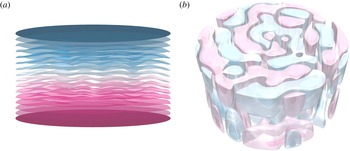
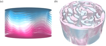
We will discuss two DNS in depth, that are representative for the two characteristic forms of rapidly rotating convection in a liquid metal in our considered parameter range. They are visualised by their temperature
 $T$
and the azimuthal velocity
 $u_{\unicode[STIX]{x1D719}}$
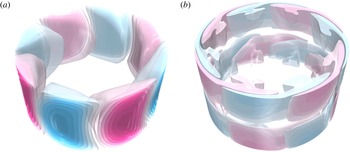
in figures 8 and 9, respectively, and in the corresponding movies 6 and 7. The first one is in the purely oscillatory regime at
 $Ro=0.115$
,
 $Ra=8.08\times 10^{5}$
, and
 $Pr=0.025$
, which means
 $Ek=2\times 10^{-5}$
. The case is close to onset, i.e.
 $Ra=1.29Ra_{o}^{a}$
. As seen in figure 8(a), the temperature shows only small deviations from the conductive state but in the form of wavy oscillations. On the other hand, the velocity field in figure 8(b), visualised by its azimuthal component, is comparatively complex, and, unlike water discussed in § 3, it is evidently not dominated by a single mode. This is characteristic for small-
 $Pr$
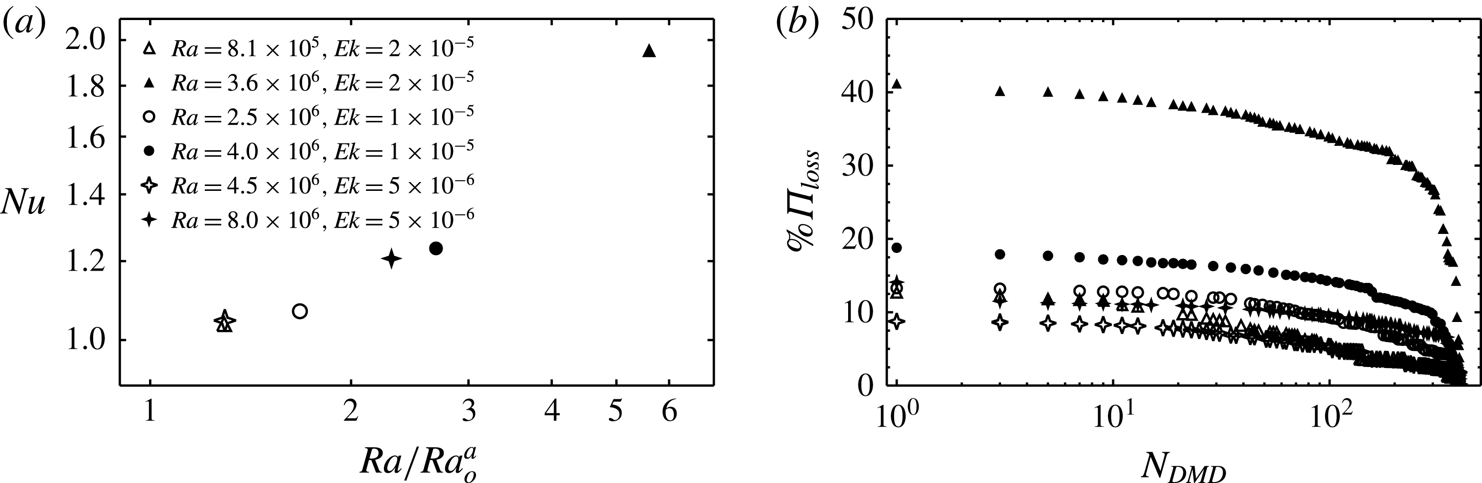
fluids. Due to the thermal diffusivity being much greater than the viscosity, the rather large velocity fluctuations are not strongly correlated with the temperature field and, as a consequence, the heat transport is not efficient. The latter is even further suppressed by the rotational constraint. The Nusselt number
 $Nu$
as a function of
 $Ra/Ra_{o}^{a}$
is shown in figure 10. Here
 $Nu=1.04$
. The second case is at a comparable Rossby number,
 $Ro=0.089$
, and a Rayleigh number above wall-mode onset, i.e.
 $Ra=1.23Ra_{w}$
. That is,
 $Ra=8.0\times 10^{6}=2.30Ra_{o}^{a}$
,
 $Pr=0.025$
and, hence,
 $Ek=5\times 10^{-6}$
. The Nusselt number is
 $Nu=1.21$
. The temperature
 $T$
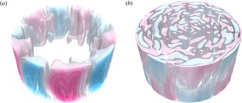
, visualised in figure 9(a), shows clear signs of a wall mode; however, it is not that apparent in the azimuthal velocity field
 $u_{\unicode[STIX]{x1D719}}$
in figure 9(b). Instead, the interior is filled with an irregular pattern of oscillatory columns and cylinder-scale inertial waves, though wall-mode-like features are also present.
Instantaneous isosurfaces obtained by DNS for
 $Pr=0.025,\;Ra=8.1\times 10^{5},\;Ek=2\times 10^{-5}$
, i.e. in the purely oscillatory regime; (a) the temperature
 $T$
, (b) the azimuthal velocity
 $u_{\unicode[STIX]{x1D719}}$
. The isosurfaces are equidistantly distributed between
 $[T_{t},T_{b}]$
and
 $[-\text{max}\,|u_{\unicode[STIX]{x1D719}}|,\text{max}\,|u_{\unicode[STIX]{x1D719}}|]$
, respectively. See also the supplementary movie 6.

Similar to figure 8 but for
 $Pr=0.025,\;Ra=8.0\times 10^{6},\;Ek=5\times 10^{-6}$
, i.e. when wall modes and oscillatory modes coexist. Isosurfaces for (a) the temperature
 $T$
, (b) the azimuthal velocity
 $u_{\unicode[STIX]{x1D719}}$
. See also the supplementary movie 7.

(a) Nusselt number
 $Nu$
as a function of the Rayleigh number
 $Ra$
normalised by the critical
 $Ra$
for the onset of oscillatory convection
 $Ra_{a}^{o}$
according to (5.3) for
 $Pr=0.025$
. Empty symbols correspond to purely oscillatory cases, filled ones to cases where additionally wall modes are present. (b) Performance loss as a function of the number of retained DMD modes. Symbols correspond to the same cases as in figure (a).

Visual evidence already suggests that the flow in liquid metals is multi-modal and dynamically very rich, even close to onset. But we remark that in none of the simulations were any signs of quasi-steady columns found as they are typical for moderate-
 $Pr$
fluids (e.g. Horn & Shishkina Reference Horn and Shishkina2014). Instead, for
 $Ra=3.6\times 10^{6}$
and
 $Ek=2\times 10^{-5}$
with
 $Nu=1.95$
, i.e. well below
 $Ra_{s}$
, the flow is already geostrophically turbulent.
DMD amplitudes
 $|a_{k}|$
versus absolute value of the normalised frequencies
 $\widetilde{\unicode[STIX]{x1D714}}$
. The grey circles are for all DMD modes, the black circles are for the ten dominant modes, the filled symbols are for
 $\unicode[STIX]{x1D6F1}_{loss}\leqslant 10\,\%$
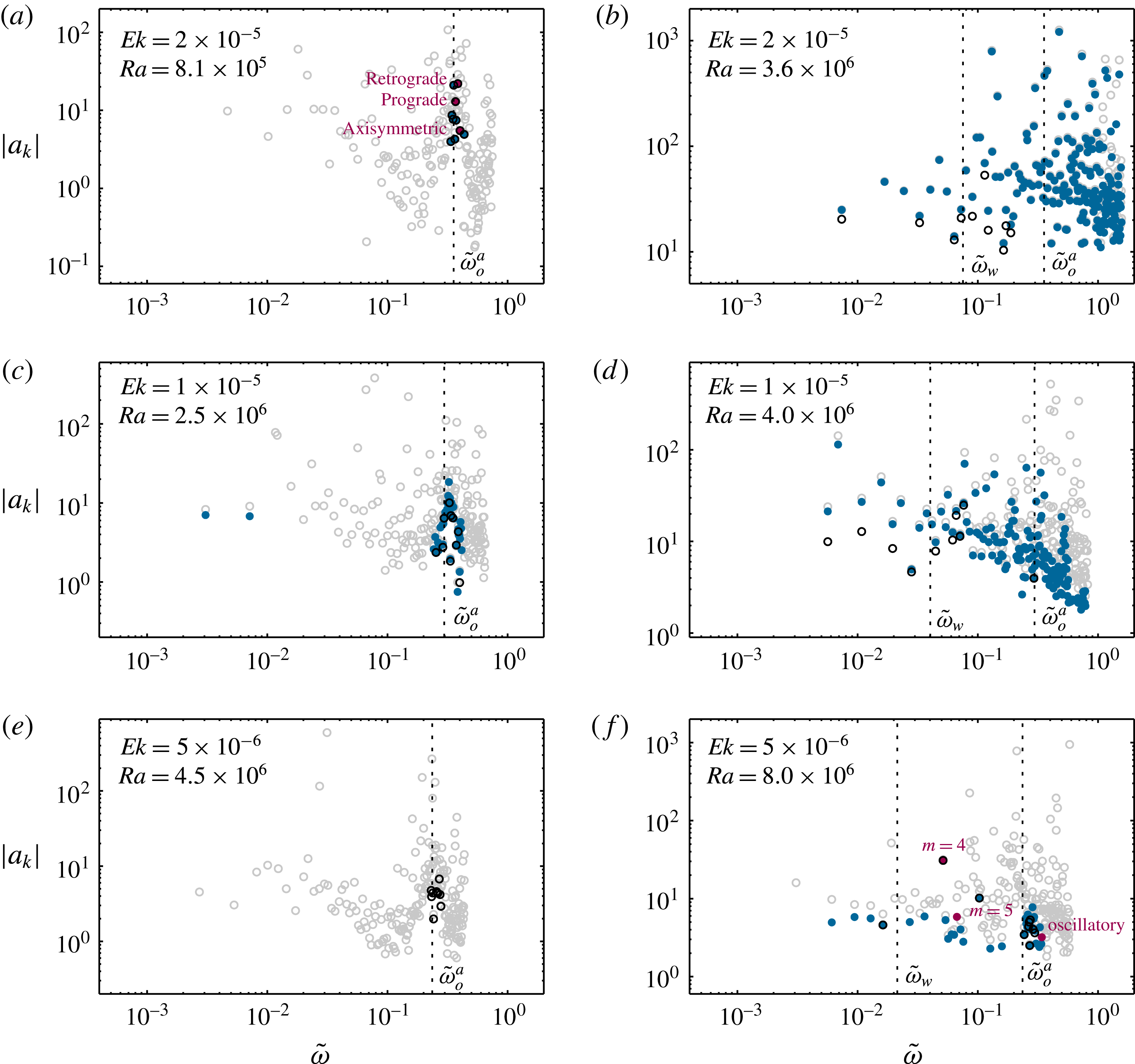
. In addition, characteristic modes that are visualised in figures 12–14 and 15–17 and shown in the supplementary movies 8–13, are marked in figures (a) and (f). The vertical dotted lines indicate the theoretical predictions for the oscillatory and wall-mode onset frequencies,
 $\widetilde{\unicode[STIX]{x1D714}}_{o}^{a}$
and
 $\widetilde{\unicode[STIX]{x1D714}}_{w}$
, according to (3.2) and (5.5), respectively.

5.3 Dynamic modes
With the sparsity-promoting variant of DMD we can quantify and characterise the flows in liquid metals in more detail. We have used
 $400$
snapshots with a sampling rate of
 $f_{s}=1$
and performed the DMD for all DNS. In figure 10(b) we show
 $\%\unicode[STIX]{x1D6F1}_{loss}$
as a function of the number of retained dynamic modes
 $N_{DMD}$
. As pointed out in § 2.2, modes extracted from real-valued data appear either as conjugate-complex dynamic mode pairs or as dynamically irrelevant zero frequency modes, here the first mode is always the mean flow. Hence, for example,
 $N_{DMD}=21$
corresponds to ten unique DMD modes. Contrary to the simulations in water (see figure 1
b) and in SF
 $_{6}$
(see figure 4
a), the decrease in
 $\%\unicode[STIX]{x1D6F1}_{loss}$
is not very steep. Nonetheless, typically a few modes still suffice to describe the flow accurately in a least-squares sense.
In figure 11 we show the full DMD spectra and indicate on the one hand the first ten dominant dynamic modes and on the other hand the modes for a fixed accuracy of
 $\%\unicode[STIX]{x1D6F1}_{loss}\leqslant 10\,\%$
. Furthermore, the predictions for the onset frequencies by oscillatory inertial and by wall-localised travelling waves according to (5.5) and (3.2) are shown. In the purely oscillatory simulations, nearly all dominant modes have high frequencies very close to
 $\widetilde{\unicode[STIX]{x1D714}}_{c}^{a}$
. Only for the simulations at a higher criticality, at
 $Ra=2.5\times 10^{6}=1.68Ra_{o}^{a}$
and
 $Ek=1\times 10^{-5}$
, few low-frequency modes are selected which correspond to body modes. For the mixed oscillatory and wall-mode simulations, the most dominant modes are low-frequency modes that are also close to the theoretical predictions for
 $\widetilde{\unicode[STIX]{x1D714}}_{w}$
. Not all modes are retrograde; in fact, there are also prograde modes.
Nonetheless, the high-frequency modes are just about as important, and for
 $Ra=3.6\times 10^{6}=0.23Ra_{s}^{\infty }$
and
 $Ek=2\times 10^{-5}$
, the spectrum is almost entirely broadband. The broadband signal suggests that the simulation is in the range of weakly or emerging geostrophic turbulence, despite being well below
 $Ra_{s}^{\infty }$
. This is in agreement with the results obtained by Aurnou et al. (Reference Aurnou, Calkins, Cheng, Julien, King, Nieves, Soderlund and Stellmach2015) (see their figure 14), who found developed geostrophic turbulence for
 $Pr=0.0235$
at the critical Rayleigh number by numerically solving asymptotically reduced equations for rapidly rotating convection (see e.g. Sprague et al.
Reference Sprague, Julien, Knobloch and Werne2006). Evidence for the onset of geostrophic turbulence below
 $Ra_{s}^{\infty }$
was also found experimentally by Bertin et al. (Reference Bertin, Grannan, Vogt, Horn and Aurnou2017) for very similar control parameters to the DNS presented here.
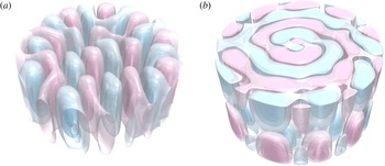
Isosurfaces of the real part of (a) the temperature
 $T$
and (b) the azimuthal velocity
 $u_{\unicode[STIX]{x1D719}}$
of a retrograde DMD mode for
 $Ra=8.1\times 10^{5},\;Ek=2\times 10^{-5},\;Pr=0.025$
. The isosurfaces are equidistantly distributed between
 $[-\text{max}\,|\text{Re}(\unicode[STIX]{x1D713}(T))|,\text{max}\,|\text{Re}(\unicode[STIX]{x1D713}(T))|]$
and
 $[-\text{max}\,|\text{Re}(\unicode[STIX]{x1D713}(u_{\unicode[STIX]{x1D719}}))|,\text{max}\,|\text{Re}(\unicode[STIX]{x1D713}(u_{\unicode[STIX]{x1D719}}))|]$
, respectively. See also the supplementary movie 8.

Similar to figure 12, but for a prograde mode. See also the supplementary movie 9.

Similar to figure 12, but for the axisymmetric oscillatory mode. (a,b) At the beginning of the oscillation period; (c,d) at half of the oscillation period. See also the supplementary movie 10.

In the following, we will discuss the modes for the previously mentioned representative cases in detail, with the spectra shown in figures 11(a) and 11(f), respectively.
In the oscillatory case, only ten modes guarantee a loss rate of less than
 $10\,\%$
, here
 $\%\unicode[STIX]{x1D6F1}_{loss}=9.75\,\%$
. Their frequencies are all very close to the theoretical prediction of
 $\widetilde{\unicode[STIX]{x1D714}}=0.356$
. Most of these modes, including the most dominant one, are retrograde precessing large-scale body modes with oscillatory columns, as visualised in figure 12 and in movie 8; but prograde modes exist as well, shown in figure 13 and in movie 9. This is in general accordance with the results of Goldstein et al. (Reference Goldstein, Knobloch, Mercader and Net1994), who predicted a multitude of modes that have critical Rayleigh numbers very close to each other and prograde modes being very likely for small-
 $Pr$
fluids. In the prograde case, it is apparent that the hot oscillatory columns get shielded by cold fluid and the cold oscillatory columns get shielded by hot fluid. Furthermore, the oscillation is also observable from the azimuthal velocity field, i.e. if the upper part of the oscillatory column has a left-handed motion, then the lower part is right-handed, and vice versa.
Even more extraordinary, we found an approximately axisymmetric torsional mode, i.e. an
 $m=0$
mode consisting of concentric circular structures with radial wavenumber of
 $l=2$
, presented in figure 14. Also in this case, oscillatory columns are simultaneously present. As seen in movie 10, the mode essentially does not precess in the azimuthal direction and also shows no travelling in the radial direction. Instead, the mode completely collapses at one quarter of a period, entirely rebuilds itself at half a period (but with the opposite sign in the temperature and the azimuthal velocity field), disintegrates again at three quarters and is then restored to its original form after one full period. This type of mode cannot be the preferred onset mode for the considered geometry and Prandtl number, according to Goldstein et al. (Reference Goldstein, Knobloch, Mercader and Net1994) and Zhang & Liao (Reference Zhang and Liao2009). However, the fact that it belongs to the important dynamic modes might suggest that, for particular parameter combinations, its growth rate can be sufficiently high to render the mode predominant. Typically, these torsional modes are associated with spherical geometries (Sánchez, Garcia & Net Reference Sánchez, Garcia and Net2016) and magnetohydrodynamic flows (Gillet et al.
Reference Gillet, Jault, Canet and Fournier2010) and are very common in geophysical settings, but here they arise very naturally in a purely thermally driven convection set-up in a cylinder.
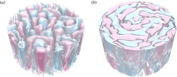
Isosurfaces of the real part of (a) the temperature
 $T$
and (b) the azimuthal velocity
 $u_{\unicode[STIX]{x1D719}}$
of a retrograde
 $m=4$
DMD wall mode for
 $Ek=5\times 10^{-6},\;Ra=8.0\times 10^{6},\;Pr=0.025$
. The isosurfaces are equidistantly distributed between
 $[-\text{max}\,|\text{Re}(\unicode[STIX]{x1D713}(T))|,\text{max}\,|\text{Re}(\unicode[STIX]{x1D713}(T))|]$
and
 $[-\text{max}\,|\text{Re}(\unicode[STIX]{x1D713}(u_{\unicode[STIX]{x1D719}}))|,\text{max}\,|\text{Re}(\unicode[STIX]{x1D713}(u_{\unicode[STIX]{x1D719}}))|]$
, respectively. See also the supplementary movie 11.

Similar to figure 15, but for a retrograde
 $m=5$
DMD wall mode coupled to an oscillatory body mode. See also the supplementary movie 12.

Similar to figure 15, but for a pure oscillating DMD mode. See also the supplementary movie 13.

In the mixed oscillatory and wall-mode case, at
 $Ra=8.0\times 10^{6}$
and
 $Ek=5\times 10^{-6}$
, more DMD modes are necessary to ensure a comparable good approximation of the flow; in fact, we need
 $36$
modes for a loss rate of less than
 $10\,\%$
, more specifically,
 $\%\unicode[STIX]{x1D6F1}_{loss}=9.82\,\%$
. The flow is dominated by a retrograde precessing
 $m=4$
wall mode, shown in figure 15 and in movie 11. The mode with the second-highest amplitude is merely a higher harmonic with
 $m=8$
. Both the temperature and the velocity field are completely wall-localised in this case. The
 $m=4$
mode has a frequency of
 $\widetilde{\unicode[STIX]{x1D714}}=0.051$
which is more than twice as high as the predicted wall-mode onset frequency of
 $\widetilde{\unicode[STIX]{x1D714}}_{w}=0.021$
, as evident from figure 11(f). This suggests that, in contrast to water, the linear stability results become invalid rather quickly for Rayleigh numbers as low as
 $1.23Ra_{w}$
. This result is confirmed by experiments in liquid gallium by Bertin et al. (Reference Bertin, Grannan, Vogt, Horn and Aurnou2017) at very similar control parameters. Their temperature spectra obtained by point temperature probes also only shows a strong peak at
 $\widetilde{\unicode[STIX]{x1D714}}\approx \widetilde{\unicode[STIX]{x1D714}}_{w}$
for
 $Ra\approx Ra_{w}$
, whereas for slightly higher
 $Ra$
the obtained frequency is approximately twice as high as
 $\widetilde{\unicode[STIX]{x1D714}}_{w}$
.
The likely reason for this behaviour is nonlinear interaction and the coupling of the oscillatory modes to the wall modes. Most of the low-frequency modes carry thermally the signature of a wall mode and kinematically the one of an inertial oscillatory mode. An example is shown in figure 16 and in movie 12. The mode shows a pronounced
 $m=5$
wall-mode travelling in the retrograde direction in the temperature field; however, the velocity field shows a superposition of a wall mode and an interior oscillatory structure. In fact, the DMD modes that are close to the predicted onset frequency resemble this type of mixed mode, despite the fact that they were not selected by the sparsity-promoting algorithm and hence are not relevant for the description of the global flow dynamics.
The oscillatory modes, with one shown in figure 17 and in movie 13, are similar to the modes discussed above; all of them have frequencies close to the theoretical prediction of
 $\widetilde{\unicode[STIX]{x1D714}}_{o}^{a}=0.236$
.
The comparable amplitudes of all modes, except the most dominant
 $m=4$
mode, also demonstrate that the flow in liquid metals is multi-modal with a variety of distinct modes in a rather broad range of frequencies, even only slightly above criticality and well below the stationary onset. Ultimately, this will give way to geostrophic turbulence. However, the regular pattern of convective Taylor columns – the well-known feature of rotating convection in moderate-
 $Pr$
fluids – is entirely missing.
6 Summary and concluding remarks
We have investigated the flow structures in rotating Rayleigh–Bénard convection in different fluids with an emphasis on liquid metals by utilising the dynamic mode decomposition (DMD) (Schmid Reference Schmid2010). DMD is an effective tool to analyse flows and thereby understand their fundamental physics. In its sparsity-promoting variant, DMD is able to rank structures by their importance to the entire flow dynamics, and, in line with this, fix the accuracy of approximation given by a superposition of a subset of the dynamic modes. One of the major advantages of DMD over POD that we have exploited here is that the extracted structures not only have a single frequency content, but that we are able to predict their temporal evolution. We have shown, moreover, that it is the complex phase between the real part and the imaginary part of the dynamic modes that determines the direction of travel. In the case of rotating convection in cylindrical containers a simple criterion was derived to decide whether the precession is prograde or retrograde.
For validation purposes, we have first applied DMD to the well-understood example of rotating convection in a fluid with
 $Pr=6.4$
, corresponding to water, in a tank with an aspect ratio
 $\unicode[STIX]{x1D6E4}=2$
, rotating with a constant
 $Ek=2.3\times 10^{-5}$
, and varying the Rayleigh number between
 $1.55\times 10^{5}\leqslant Ra\leqslant 2.60\times 10^{6}$
. For moderate
 $Ra$
a few dynamic modes suffice to accurately describe the flow. In agreement with previous experiments by Zhong et al. (Reference Zhong, Ecke and Steinberg1991, Reference Zhong, Ecke and Steinberg1993) and linear theory by Goldstein et al. (Reference Goldstein, Knobloch, Mercader and Net1993), we found that, close to onset, convection occurs by wall-localised retrograde precessing waves whose frequency increases linearly with
 $\unicode[STIX]{x1D700}$
, indicating that they originated from a Hopf bifurcation. With increasing Rayleigh number
 $Ra$
, the interior of the container gradually fills with columnar vortices. These result in mixed modes, with the bulk and the wall region having the same frequency content, i.e. they do not get separated by the DMD. Eventually, for the highest
 $Ra$
investigated here, the well-known regular pattern of convective Taylor columns prevails.
As a second example, we studied rotating RBC in a
 $Pr=0.8$
fluid confined in a cylinder with
 $\unicode[STIX]{x1D6E4}=0.5$
, for two specific rotation rates
 $Ro=0.3$
and
 $Ro=0.5$
. In this case, the dominant structure is an
 $m=1$
body mode; however, the small change in
 $Ro$
leads to either a prograde or a retrograde precession. Thus, it constitutes an ideal case to corroborate that it is the complex argument of the dynamic modes that contains the information about the direction of travel.
In the third and main part, we considered thermal convection in a fluid with
 $Pr=0.025$
corresponding to a liquid metal at rapid rotation rates of
 $Ek=2\times 10^{-5}$
,
 $1\times 10^{-5}$
, and
 $5\times 10^{-6}$
, respectively. In contrast to moderate-
 $Pr$
flows, we demonstrated that there is a variety of distinct modes already close to onset in this case. A comparatively small variation of
 $Ra$
, i.e. less than a decade, yields a significant change of the flow morphology. DMD proved to be especially well suited for these low-
 $Pr$
flows, since there exist various inherent instability processes that are linked to characteristic frequencies. The two archetypes occurring in the considered parameter range describe (i) purely oscillatory convection and (ii) mixed oscillatory and wall-mode convection. We discussed them on two examples in more detail. For
 $Ra=8.1\times 10^{5}$
and
 $Ek=2\times 10^{-5}$
, the oscillatory case, DMD revealed that there are simultaneously pronounced prograde and retrograde modes. Kinematically they appear as cylinder-scale inertial waves, thermally as oscillatory columns. Moreover, we obtained a quasi-axisymmetric torsional mode, which is the first observation of this type of mode in a cylinder. All the dynamic modes show high frequencies close to the predicted onset frequency according to Zhang & Liao (Reference Zhang and Liao2009). For
 $Ra=8.0\times 10^{6}$
and
 $Ek=5\times 10^{-6}$
, in the mixed-mode case, we found that low-frequency wall modes dominate the flow. Furthermore, there are also oscillatory inertial modes present, very similar to the purely oscillatory case. Some of these mixed modes consist of a nonlinear superposition of wall modes and inertial modes. The flow is hence multi-modal at very low supercriticality. With increasing
 $Ra$
, the flow becomes more chaotic and ultimately gives way to geostrophic turbulence, likely before the classical prediction for the stationary onset (Aurnou et al.
Reference Aurnou, Calkins, Cheng, Julien, King, Nieves, Soderlund and Stellmach2015; Bertin et al.
Reference Bertin, Grannan, Vogt, Horn and Aurnou2017).
DMD is equally applicable to flow fields that are obtained experimentally, e.g. by PIV (Schmid Reference Schmid2010; Schmid et al. Reference Schmid, Li, Juniper and Pust2011). However, their acquisition is extremely difficult for convection in visually opaque liquid metals, rather data typically comes from point-wise measurements. DNS in combination with DMD is invaluable here since it allows us to directly link frequencies, e.g. from time series of temperatures, to an actual flow structure. A comparative study with laboratory experiments in liquid gallium to demonstrate this point is planned.
Considering rotating RBC in a
 $Pr=0.025$
fluid as a proxy for convection in the liquid cores of planets, our findings suggest that convective Taylor vortices are unlikely to be responsible for planetary dynamos, as these structures are completely absent in our simulations. Yet, they are the key ingredient of most present-day dynamo models (Christensen Reference Christensen2011; Jones Reference Jones2011). This is consistent with the fact that the typical length scale of Taylor columns in their primary form is too small, as they scale with
 $Ek^{1/3}$
(Aurnou & King Reference Aurnou and King2017).
However, this does not rule out that columnar large-scale vortices (LSVs) are formed through an inverse cascade (Julien et al.
Reference Julien, Rubio, Grooms and Knobloch2012b
; Favier, Silvers & Proctor Reference Favier, Silvers and Proctor2014; Guervilly, Hughes & Jones Reference Guervilly, Hughes and Jones2014; Rubio et al.
Reference Rubio, Julien, Knobloch and Weiss2014; Stellmach et al.
Reference Stellmach, Lischper, Julien, Vasil, Cheng, Ribeiro, King and Aurnou2014; Aurnou et al.
Reference Aurnou, Calkins, Cheng, Julien, King, Nieves, Soderlund and Stellmach2015; Kunnen et al.
Reference Kunnen, Ostilla-Mónico, van der Poel, Verzicco and Lohse2016). In fact, our simulations are suggestive that the formation of LSVs is facilitated in a low-
 $Pr$
fluid, because the pathway to geostrophic turbulence is not through convective Taylor columns that first have to loose their sleeves (Julien et al.
Reference Julien, Rubio, Grooms and Knobloch2012b
). Simulations at higher
 $Ra$
and, hence, deeper in the geostrophically turbulent regime, will be subject to future studies and will enable us to test this hypothesis. Nevertheless, using the estimates of
 $Pr_{\oplus }\sim 10^{-2}$
and
 $Ek_{\oplus }\sim 10^{-15}$
for Earth’s core yields critical Rayleigh number estimates of
 $Ra_{s}^{\infty }\sim 9\times 10^{20}$
and
 $Ra_{o}^{\infty }\sim 4\times 10^{18}$
. Thus, assuming a core Rayleigh number of
 $Ra_{\oplus }\approx 10^{20}$
, we argue that the DNS results presented here might be close to the correct regime, at least, in terms of supercriticality.
On the other hand, we find that convection in
 $Pr=0.025$
exhibits many of the features not only found in the core, but also in many other low-
 $Pr$
geo- and astrophysical settings. These are, for example, the low-frequency wall modes that modulate the oscillatory waves, that resemble the large-scale modulation of waves at the core–mantle boundary, the retrograde drift of the magnetic flux patches that is likely associated with the motion in the fluid part of the Earth’s core (Finlay & Jackson Reference Finlay and Jackson2003; Hori, Jones & Teed Reference Hori, Jones and Teed2015), the prograde motion of waves in the Sun (Gizon & Birch Reference Gizon and Birch2005) and even the torsional modes (Gillet et al.
Reference Gillet, Jault, Canet and Fournier2010; Roberts & Aurnou Reference Roberts and Aurnou2012). Typically, these motions are all associated with systems that are strongly influenced by magnetic fields; however, here we have shown that such behaviour can appear in a purely thermal set-up. Thus, understanding the flow, in particular, the coherent flow structures in the present very basic configuration, is essential and a necessary first step for gaining more insight into the far more complex geophysical and astrophysical flows.
Acknowledgements
S.H. acknowledges funding by the Deutsche Forschungsgemeinschaft (DFG) under grant HO 5890/1-1 and the NSF Geophysics Program, award no. 1547269. We also gratefully acknowledge the Leibniz-Rechenzentrum in Garching for providing computational resources on SuperMUC.
Supplementary movies
Supplementary movies are available at https://doi.org/10.1017/jfm.2017.631.